Review

A Review of Decision-Making and Planning for Autonomous Vehicles in Intersection Environments

1
School of Traffic &Transportation, Chongqing Jiaotong University, Chongqing 400074, China
2
Chongqing YouLiang Science & Technology Co., Ltd., Chongqing 401336, China
3
Chongqing Zongheng Engineering Design Co., Ltd., Chongqing 401124, China
*
Author to whom correspondence should be addressed.
World Electr. Veh. J. 2024, 15(3), 99; https://doi.org/10.3390/wevj15030099
Submission received: 23 December 2023 / Revised: 26 February 2024 / Accepted: 4 March 2024 / Published: 6 March 2024

Abstract

:
Decision-making and planning are the core aspects of autonomous driving systems. These factors are crucial for improving the safety, driving experience, and travel efficiency of autonomous vehicles. Intersections are crucial nodes in urban road traffic networks. The objective of this study is to comprehensively review the latest issues and research progress in decision-making and planning for autonomous vehicles in intersection environments. This paper reviews the research progress in the behavioral prediction of traffic participants in terms of machine learning-based behavioral prediction, probabilistic model behavioral prediction, and mixed-method behavioral prediction. Then, behavioral decision-making is divided into reactive decision-making, learning decision-making, and interactive decision-making, each of which is analyzed. Finally, a comparative analysis of motion planning and its applications is performed from a methodological viewpoint, including search, sampling, and numerical methods. First, key issues and major research progress related to end-to-end decision-making and path planning are summarized and analyzed. Second, the impact of decision-making and path planning on the intelligence level of autonomous vehicles in intersecting environments is discussed. Finally, future development trends and technical challenges are outlined.

1. Introduction

With social and economic development, as well as technological progress, the number of vehicles on the road is increasing exponentially. While people enjoy the convenience, speed, and comfort of travel, they face increasingly serious problems, such as traffic congestion [1], accidents [2], and environmental pollution [3]. Autonomous driving technologies have emerged to improve traffic safety and traffic flow while providing economic benefits, environmental protection, and social inclusion [4]. Urban intersections significantly affect the safe and efficient operation of urban traffic. In the case of conventional manual driving traffic flows, intersections are the sites of most urban traffic accidents [5]. Therefore, decision-making and planning of autonomous vehicles (AVs) at intersections are important.
Decision-making and planning for autonomous driving at intersections constitute a complex problem involving multiple factors, such as traffic signals, the positions and speeds of other vehicles and pedestrians, road signs and markings, and the vehicle’s sensors and computational capabilities. This problem can be divided into three layers: environmental perception, decision planning, and control execution, as shown in Figure 1.
An automatic driving system consists of three layers: environmental awareness, decision-making, and control execution [6]. The environmental-sensing layer is responsible for sensing rich information and providing control instructions to the control–execution layer based on driving tasks and control objectives. The decision-making layer can be of two types: hierarchical and end-to-end. Hierarchical tasks are divided into precise and clear orders and have a good stepwise reasoning ability. The end-to-end approach employs a straightforward architecture that effectively addresses the challenges of presenting intricate scene features [7].
The purpose of this paper is to provide an overview of research progress in the area of decision-making and planning for self-driving vehicles at intersections, as well as future trends and technical challenges. Specific research goals include:
1. Behavior Prediction: It explores how environmental awareness techniques and machine learning algorithms can be used to accurately predict the behavior of other vehicles and pedestrians at intersections. This includes identifying and tracking road users and predicting their intentions and behaviors so that self-driving vehicles can make decisions accordingly.
2. Behavioral Decision-Making: It investigates how to develop behavioral decision-making strategies for self-driving vehicles at intersections based on perception results and traffic rules, considering factors such as traffic flow, safety, and efficiency. This includes selecting appropriate traffic signal control methods in different traffic scenarios, merging and separating traffic flows, and coordinating with other road users.
3. Path Planning: It investigates how to achieve the safe, efficient, and smooth movement of self-driving vehicles through intersections through path planning and motion control. This includes optimal path selection, speed control, vehicle maneuvering, etc., to ensure that the vehicle can safely navigate intersections and adapt to complex traffic environments.
4. End-to-End Decision-Making and Planning: It analyzes the potential and limitations of an end-to-end approach to the application of autonomous driving at intersections. This approach integrates perception, decision-making, and planning into a unified model to learn driving strategies and behavioral planning directly from raw sensor data using deep learning techniques.
By summarizing the research progress in the field of decision-making and planning for self-driving vehicles at intersections, it can provide a reference for related researchers and practitioners to promote the development of the application of self-driving technology at intersections and address the challenges faced.

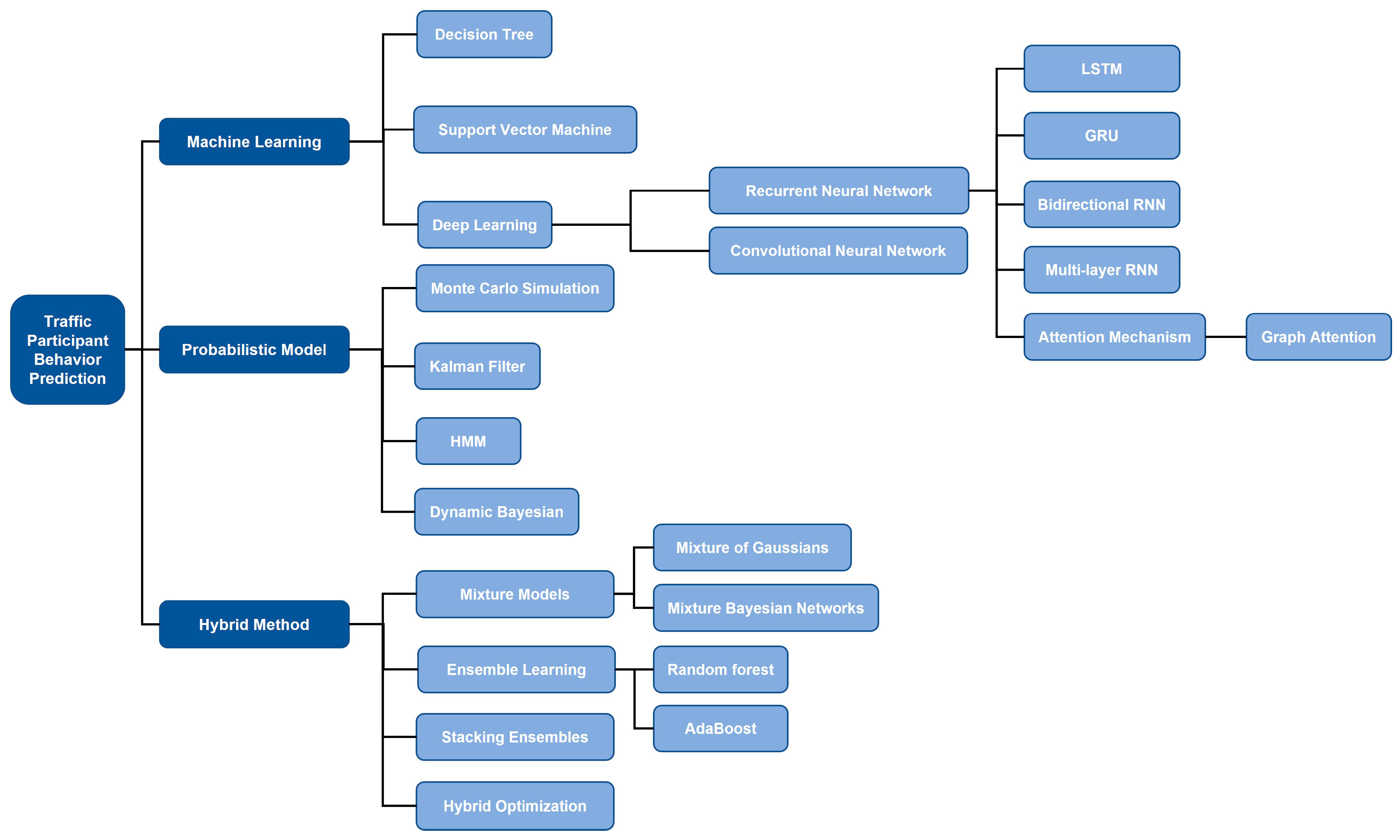
2. Behavioral Prediction of Traffic Participant

The prediction of intersection traffic participant behavior can be categorized into three research methods: machine learning-based methods, probabilistic model-based methods, and hybrid method-based methods [8]. This section reviews these three research methods. Figure 2 provides details on the subclasses included in machine learning, probabilistic modeling, and hybrid methods.

2.1. Machine Learning

Machine-learning methods are used to make predictions by learning pedestrian behavior patterns from large amounts of data. Common machine-learning methods include decision trees, random forests, support vector machines, and deep learning. These methods extract information from features such as movement trajectories, posture, and appearance of traffic participants and use supervised or reinforcement learning algorithms for training and prediction. However, the quality of data parsing and cleaning significantly affects the prediction accuracy.
A decision tree is a classification and regression model based on a tree structure that is constructed by recursively partitioning the input dataset, where each internal node represents a feature or attribute, and each leaf node represents a category or value. Wang et al. [9] proposed a stochastic decision tree-based method for predicting lane-change driving angles. The method was validated by constructing a random decision tree to predict the driving angle with input variables of relative speed, relative acceleration, and potential. The validation was performed using the NGSIM dataset.
The decision tree has the following advantages and disadvantages. The advantages are the following: (1) Interpretability: decision trees have a clear structure that can visually represent the importance of features and the decision-making process, which is easy to understand and interpret. (2) Non-parametric: Decision trees do not make assumptions about the distribution of data in the modeling process and do not require prior normalization or standardization of data. (3) Robustness: Decision trees are robust to outliers and missing data and can handle data sets with noise or missing values. The disadvantages are the following: (1) Easily overfitted: Decision trees are prone to overcomplicated fitting of training data, resulting in the poor generalization of new data. (2) Local optimization problem: the decision tree construction process is based on the local optimal division strategy, which may lead to the obtained decision tree not being the global optimal. (3) Sensitivity to changes in input data: small changes in the decision tree to the input data may lead to significant changes in the tree structure, making it unstable. (4) Difficulty in dealing with high-dimensional data: when the number of features is large, the construction of the decision tree and the search space will become very large, requiring high computational resources.
Support vector machine (SVM) is a common supervised learning algorithm mainly used for classification and regression problems. The basic idea of SVM is to divide or regress data by finding an optimal hyperplane in the feature space. Li et al. [10] selected vehicle speed, acceleration, and distance from red light start time to stop line as classification attributes and used unweighted and weighted least squares support vector machine (LS-SVM) to solve the red-light running prediction problem. Rahman et al. [11] used linear support vector machines and polynomial support vector machines to process vehicle attribute data (e.g., speed, location, and arrival time) collected at the onset of the yellow indication and ultimately predicted the driver’s stop-and-go decision based on the data.
SVM has the following advantages and disadvantages. The advantages are the following: (1) Effective in high-dimensional spaces: by using kernel functions, SVM can perform nonlinear classification and regression in high-dimensional feature spaces. (2) Good generalization ability: SVM finds the optimal hyperplane by maximizing the interval, which helps reduce the risk of overfitting and has good generalization ability. (3) Good performance for datasets with small feature dimensions: SVM can provide good performance when the feature dimensions are small. (4) Better robustness to outliers: since SVM mainly focuses on the support vectors on the boundary, it has less effect on outliers. The disadvantages are the following: (1) Longer training time for large-scale datasets: the training time of SVM increases with the size of the dataset, especially when using nonlinear kernel functions. (2) Need to choose appropriate kernel functions and hyperparameters: choosing the appropriate kernel functions and hyperparameters is critical to the performance of SVMs.
RNN stands for Recurrent Neural Network. Unlike traditional feed-forward neural networks, RNNs have temporal recurrent connectivity, enabling them to process sequential data and tasks with temporal dependencies. RNN models include several common variants and extensions of the following: Long Short-Term Memory (LSTM) network, Gated Recurrent Unit (GRU), Bidirectional RNN, Multi-layer RNN, and Attention Mechanism [12].
Zhou et al. [13] combined the historical trajectories of pedestrians, signalized intersection phase data, and risk factors to predict pedestrian trajectories at signalized intersections. Intersection phase data and risk factors were used as inputs for the LSTM model to predict future trajectories of pedestrians. Li et al. [14] established a bidirectional LSTM (BiLSTM) and GRU to solve the long-distance dependence and reduce overfitting to improve the prediction accuracy of electric vehicle speed. Cao et al. [15] developed a multi-layer LSTM model to predict the trajectories of target vehicles at intersections with straight, left, and right turns. Lian et al. [16] developed an attention-based LSTM (CA-LSTM) model and combined it with the dynamic features of pedestrians to predict whether they would cross a road with 89.68% accuracy. Alghodhaifi et al. [17] proposed a graph-based trajectory prediction model for pedestrian–vehicle interactions called holistic spatio-temporal graph attention (HSTGA), which accurately predicts pedestrian trajectories at unsignalized intersections. Ji [18] extracted spatio-temporal features using an LSTM network and a graph attention network (GAT) for the prediction of vehicle trajectory states at intersections. Yao et al. [19] used GAT-LSTM to study the interaction between motorized vehicles and motorcycles, as well as the predicted trajectories and head-on orientations of vehicles during left-turning vehicle–motorcycle encounters.
The LSTM network has the following advantages and disadvantages. The advantages are the following: (1) Long-term memory capability: LSTM effectively solves the long-term dependency problem through the gating mechanism and can memorize and process long-term sequence information. (2) Anti-gradient vanishing: LSTM uses the gating mechanism, which can effectively mitigate the gradient vanishing problem, enabling the network to better train and learn long sequences. (3) Flexibility: the structure of LSTM can be flexibly designed and extended according to the task requirements, such as stacking multiple LSTM layers or combining them with other types of layers. The disadvantages are the following: (1) Computational complexity: the LSTM is more computationally intensive compared with the traditional RNN model and requires more computational resources. (2) Larger number of parameters: LSTM introduces additional gating mechanisms and state variables, which increases the number of parameters in the model and requires more storage space for training and inference. (3) Hyperparameter adjustment: LSTM has multiple hyperparameters, such as the number of hidden units, learning rate, etc., and adjusting these hyperparameters takes time and computational resources.
The GRU has the following advantages and disadvantages. The advantages are the following: (1) Simplified structure: GRU simplifies the structure of the gating unit and reduces the number of parameters compared with LSTM, which makes the training and inference of the network faster. (2) Fewer gating units: GRU has only two gating units, an update gate and a reset gate, which is more concise compared with the three gating units of LSTM. (3) Good performance: GRU performs similarly to LSTM on some tasks and even better sometimes. The disadvantages are the following: (1) Larger number of parameters: The number of parameters of the GRU model is relatively large, resulting in more storage space required for training and inference. (2) Difficult to interpret: the internal operation mechanism of GRU is relatively complex, and it is not easy to understand the specific process and decision logic.
The Bidirectional RNN has the following advantages and disadvantages. The advantages are the following: (1) Contextual information enrichment: the Bidirectional RNN considers both past and future contextual information and can better capture relevant features in the sequence. (2) Better representation: the Bidirectional RNN provides a more comprehensive and richer representation of features by combining forward and reverse information. The disadvantages are the following: (1) Computational complexity: the Bidirectional RNN needs to run two RNNs in both forward and reverse directions, increasing the amount of computation and training time. (2) Context symmetry: the Bidirectional RNN assumes symmetry of the forward and reverse contexts, but in some tasks, the contexts may be asymmetric, which may lead to an impact on the model performance.
The Multi-layer RNN has the following advantages and disadvantages. The advantages are the following: (1) Stronger representation ability: by increasing the number of layers of RNN, the nonlinear modeling ability of the network can be improved to better capture features in complex sequences. (2) Rich representation hierarchy: each RNN layer can extract features at different levels and gradually build a more abstract representation. The disadvantages are the following: (1) Computational complexity: Multi-layer RNN models consist of multiple RNN layers stacked together, which increases the computation and training time. (2) Gradient vanishing and explosion: in deep RNNs, the problems of gradient vanishing and gradient explosion may be more significant, and some techniques are needed to mitigate these problems.
The Attention Mechanism has the following advantages and disadvantages. The advantages are the following: (1) Contextual attention: the Attention Mechanism can pay dynamic attention to different positions in the input sequence, thus better capturing contextual information when processing sequence tasks. (2) Long-term dependency: the Attention Mechanism can help the model to process long sequences efficiently, which enables the model to better remember and use the relevant information from a long distance. (3) Interpretability: the Attention Mechanism can provide an explanation of the model’s decisions, and by visualizing the attention weights, it can understand how much attention the model pays to different parts of the model, which increases the interpretability and credibility of the model. The disadvantages are the following: (1) Computational complexity: the Attention mechanisms need to compute the attention weights, as well as weighted aggregation of features, which increases the amount of computation. (2) Context length limitation: the Attention Mechanism usually considers all the context information when computing the attention weights, which may lead to computational and storage difficulties when dealing with very long sequences.
CNN stands for Convolutional Neural Network. CNN has good feature extraction capability and can effectively capture local and global features in data such as images and text. Liang et al. [20] were able to correctly predict the intentions of pedestrians and cyclists by building a CNN prediction model with an average accuracy of 84.96% and an absence trigger rate of 0.037%. Sun et al. [21] proposed a Conv-LSTM model for predicting the position of a left-turning vehicle at an intersection during a turn, which employs CNNs to extract behavioral features at different times.
CNN has the following advantages and disadvantages. The advantages are the following: (1) Local feature extraction: CNN can effectively extract local features in images or videos and has a good ability to model the local behavioral patterns of vehicles, pedestrians, and other participants in traffic scenes. Through the filter operation of the convolutional layer, CNN can capture visually important spatial features. (2) Spatial invariance: the CNN has some translational invariance through the convolution and pooling operations, which is robust to the positional changes, scale changes, and translational changes of the participants in the traffic scene. Such a property allows CNN to handle image data from different camera viewpoints. (3) Modeling on time: by taking multiple image frames as inputs, CNNs can model the behavior of participants through the time dimension. By stacking multiple convolutional and recurrent layers, CNNs can capture certain temporal information to help predict the dynamics of participant behavior. (4) Parameter sharing and reduction of overfitting: CNN can reduce the number of parameters of the model and the risk of overfitting through parameter sharing and pooling operations and improve the generalization ability of the model. The disadvantages are the following: (1) Large data demand: CNN models usually require a large amount of annotated data for training, especially when dealing with complex tasks or large-scale data sets. If the available data are limited, it may cause the performance of the model to degrade. (2) Large number of parameters: With the increase in the number of network layers and the number of convolutional nuclei, the number of parameters in the CNN model will also increase. This results in models requiring more computational resources for training and reasoning, which can be challenging for resource-constrained devices. (3) Poor interpretability: Due to the complexity of CNN models, they are often difficult to explain and understand. This can be a limiting factor in some scenarios where the model needs to be explained. (4) Difficulty in hyperparameter adjustment: the CNN-LSTM model involves more hyperparameters, such as convolution kernel size and LSTM hidden unit number. Adjusting these hyperparameters may require more trial and tuning, increasing the difficulty of tuning parameters.
In summary, the prediction of traffic participant behavior using machine-learning methods has the advantages of being efficient, accurate, real-time, and adaptive, but there are also challenges and limitations in terms of data requirements, data quality, model complexity, and interpretability. These factors need to be weighed in the application, and appropriate measures need to be taken to solve the related problems.

2.2. Probabilistic Model

The probabilistic modeling of driving behavior prediction refers to the estimation of the corresponding probabilities for all possible future outcomes of a random variable, which allows behavior prediction [22]. Probabilistic modeling methods include Monte Carlo simulation, the Kalman filter, the HMM, and dynamic Bayesian network.
Monte Carlo simulation is a simulation method based on probability and stochasticity for solving complex problems or assessing uncertainty. It typically simulates the behavior of a system by generating random samples and performs statistical analysis based on these samples. Jeong [23] predicted the future behavior of vehicles approaching an intersection using a sensor-based Monte Carlo simulation prediction module.
Monte Carlo simulation has the following advantages and disadvantages. The advantages are the following: (1) Dealing with complex problems: Monte Carlo simulation can be used to solve complex problems or assess the behavior of complex systems, even if these problems or systems do not have explicit analytical solutions. (2) Unrestricted distributional assumptions: Monte Carlo simulation does not require specific distributional assumptions about the data or the behavior of the system and can, therefore, be applied to a wide variety of types of problems and data. (3) Consideration of uncertainty: Monte Carlo simulation can consider uncertainty and variability in a problem by generating random samples, thus providing probabilistic information about the outcome. (4) Flexibility: Monte Carlo simulations can improve the accuracy of the results by increasing the number of samples, so the accuracy of the calculations can be adjusted as needed. The disadvantages are the following: (1) High computational cost: Monte Carlo simulation usually requires many random samples to obtain accurate results, so the computational cost is relatively high. (2) Possible sampling error: the results of Monte Carlo simulation are limited by the number of samples, and the sampling error of the samples may lead to a bias in the results. (3) Dimensionality catastrophe: in high-dimensional problems, many samples are required to adequately cover the parameter space, leading to a sharp increase in computational complexity. (4) The effect of randomness: the results of Monte Carlo simulation are affected by random samples, and different random samples may lead to slightly different results, which requires adequate sample size and statistical analysis.
The Kalman filter (KF) is an optimization filter for estimating and predicting the state of a system. It is based on a linear system model and Gaussian noise assumptions and provides an optimal estimate of the system state by recursively fusing the measured data with the predictions of the system model. Chen et al. [24] developed an adaptive KF-based model for vehicle following and merging behaviors. Qian et al. [25] proposed a two-stage quantitative adaptive KF algorithm based on an autoregressive moving average (MA) model to predict the vehicle state (including the direction of travel, lane of travel, vehicle speed, and acceleration). Tan et al. [26] used an adaptive KF and integrated K-nearest neighbor models for real-time vehicle trajectory prediction during predictive signal phase transitions.
The KF has the following advantages and disadvantages. The advantages are the following: (1) Optimality: The Kalman filter provides optimal estimates based on a linear system model and Gaussian noise assumptions. Under these assumptions, the Kalman filter obtains the minimum mean square error estimate of the system state. (2) Recursive: the Kalman filter has a recursive structure that allows real-time state estimation based on previous state estimates and measurements without the need to store large amounts of historical data. (3) Efficient: since the Kalman filter is based on a linear system model, it has relatively low computational complexity and is suitable for real-time applications and environments with limited computational resources. The disadvantages are the following: (1) Accuracy of the system model: the Kalman filter is sensitive to the accuracy of the system model, and if the model is inaccurate or the parameters are incorrectly estimated, it may lead to bias in the estimation results. (2) Dependence of initial conditions: the Kalman filter is sensitive to the choice of initial state estimation and initial covariance, and inaccurate initial conditions may affect the stability and accuracy of the estimation results.
The hidden Markov model (HMM) is a statistical model for modeling sequential data with potentially unobserved states. It is an extension of the Markov chain that models and analyzes sequential data by describing the probabilistic relationship between state sequences and observed sequences. Mao et al. [27] proposed a method for predicting pedestrian crossing violations using logistic regression and Markov chain models. Nasernejad [28] modeled and investigated the collision avoidance mechanism between pedestrians and vehicles in conflict situations using a Markov decision process (MDP) framework. Zhang et al. [29] used a Kalman filter to update the kinematic parameters of the attitude of the target vehicle. The turning behavior of the vehicle was then identified using the heading angle and acceleration components in combination with an HMM and Bayesian filtering.
The HMM has the following advantages and disadvantages. The advantages are the following: (1) Flexibility: the HMM can model sequence data with potentially unobserved states and is applicable to various types of sequence data, such as natural language, speech, and time series. It captures temporal dependencies and sequence structure in the data. (2) Probabilistic modeling: the HMM provides a probabilistic way of modeling the probabilistic relationship between system states and observations. This gives the HMM an advantage in uncertainty modeling and inference problems by providing information about the probability distribution of states and observations. (3) Sequence prediction: HMMs can be used for the prediction of sequences of future observations. By estimating the probability distribution of a given sequence of observations, the likelihood of the next observation or a future segment of the observation sequence can be predicted. (4) Interpretability: The parameters and probability distributions of the HMM can be estimated and interpreted using statistical methods. This makes the results of the HMM interpretable, revealing patterns, transitions, and associations in the sequence data. The disadvantages are the following: (1) Independence assumption: the HMM assumes that the state of the system is only related to the previous state, i.e., it satisfies the Markov property. This assumption may not be applicable to some practical situations, such as long-term dependencies or complex dependencies between states. (2) Computational complexity: In some complex problems, the computational complexity of the HMM may be high. Especially when the state space and observation space are large, many computations and storage are required and may become infeasible. (3) Parameter estimation: parameter estimation of the HMM usually depends on the quality and quantity of the observed data. When observation data are scarce or noisy, parameter estimation may become inaccurate, and more data may be required to improve the accuracy of the estimation.
Dynamic Bayesian network (DBN) is a probabilistic graphical model that extends the concept of Bayesian Networks to model dynamic systems. It allows for modeling and reasoning about systems that evolve over time by capturing dependencies between variables at different time points. Sun et al. [30] proposed a multi-agent hybrid dynamic Bayesian network (MHDBN) method that can predict the behaviors of multiple vehicles and pedestrians in various scenarios, and Xu et al. [31] proposed a method for predicting pedestrian trajectories according to a combination of pedestrian crossing behavior and intention. Pedestrian behavior was identified using a Bayesian a posteriori model, and pedestrian intention was identified using a dynamic Bayesian network. Xu [32] used a dynamic Bayesian network to integrate pedestrian group behavior and signalized crossing environment information. Subsequently, a crossing decision model and a motion model were used to predict the group trajectory in the following few seconds.
The DBN has the following advantages and disadvantages. The advantages are the following: (1) Temporal modeling: DBNs explicitly model the temporal dependencies between variables, allowing for the representation of dynamic systems and capturing their time-evolving behavior. (2) Flexibility: DBNs can handle both discrete and continuous variables, making them applicable to a wide range of domains and problems. (3) Uncertainty modeling: DBNs provide a principled way to represent and reason about uncertainty in dynamic systems by propagating probabilities through time. (4) Inference capabilities: DBNs enable various inference tasks, such as filtering, smoothing, and prediction, which can be used for state estimation and prediction in time-series data. The disadvantages are the following: (1) Computational complexity: Inference in DBNs can be computationally demanding, especially for large or complex models. Exact inference is often intractable, and approximate methods or sampling techniques may be required. (2) Model specification: Specifying the structure and parameters of a DBN can be challenging, especially for complex systems. Determining the appropriate number of hidden variables and their dependencies requires domain knowledge and expertise. (3) Data requirements: DBNs typically require enough training data to estimate the model parameters accurately. Limited or noisy data may lead to less reliable inference results. (4) Curse of dimensionality: As the number of variables and time steps increases, the size of the joint probability distribution grows exponentially, leading to the curse of dimensionality. This can make learning and inference in DBNs computationally challenging.
In summary, the use of probabilistic modeling methods for predicting traffic participant behavior has the advantages of uncertainty modeling, flexibility, and interpretability, but there are also challenges and limitations in terms of data requirements, assumption limitations, computational complexity, and prediction accuracy. These factors need to be considered comprehensively in applications, and suitable probabilistic models and methods need to be selected according to specific situations.

2.3. Hybrid Method

A hybrid approach refers to combining several different methods or models to achieve better performance or more comprehensive analysis results. Common hybrid methods include the hybrid model, ensemble learning, stacked integration, and hybrid optimization.
A hybrid model combines multiple probability distribution functions into a single model, with each distribution function corresponding to a submodule or subpopulation. By combining different sub-models in a weighted manner, data can be modeled and predicted more accurately. Common mixture models include a mixture of Gaussian and mixture Bayesian networks.
Hardy et al. [33] proposed an adaptive Gaussian mixture model (aGMM) formula for multi-step probabilistic state prediction using a non-parametric Gaussian process (GP) regression model. The proposed prediction algorithm is suitable for any dynamic system, which is difficult to model parametrically, but the data are available. The proposed adaptive GP-AGMM formula is suitable for the prediction of driver behavior at road intersections using the GP driver behavior model combined with the parametric vehicle model. Jiang et al. [34] proposed a probabilistic vehicle trajectory prediction method based on a dynamic Bayesian network (DBN) model that incorporates the driver’s intention, maneuvering behavior, and vehicle dynamics. A Gaussian mixture model-hidden Markov model was designed by selecting the most relevant feature vectors using joint mutual information, and the model was used as a node in the DBN to recognize the driver’s intention.
The mixture models have the following advantages and disadvantages. The advantages are the following: (1) Flexibility: The hybrid model is very flexible and can be adapted to various forms of data distribution. By combining multiple simple distributions, complex data distributions can be modeled, including multi-peaked distributions, asymmetric distributions, and so on. (2) Powerful: The mixture model can represent more complex data structures and generative processes, including multiple potential subpopulations or hidden states. It can capture different patterns and clusters in the data, providing more detailed data analysis and pattern recognition capabilities. (3) Probabilistic modeling: The mixture model provides probabilistic modeling of the data, allowing for the calculation of the probability that a data point belongs to each component. This allows tasks such as probabilistic inference, statistical analysis, and outlier detection. (4) Parameter estimation: Parameter estimation for mixed models can usually be performed using standard maximum likelihood estimation or Bayesian inference methods. These methods have been widely studied and applied to efficiently estimate model parameters. The disadvantages are the following: (1) Model selection: The performance and fitting ability of a mixed model is highly dependent on the choice of the number of components and distribution. The selection of an inappropriate number of components or type of distribution may lead to the overfitting or underfitting of the model, thus affecting the accuracy of the modeling results. (2) Computational complexity: the computational complexity of hybrid models is usually high, especially in the case of high-dimensional data or large datasets. (3) Initial value sensitivity: the parameter estimation for hybrid models usually requires the selection of appropriate initialization values. Inappropriate initialization values may cause the algorithm to fall into a local optimum solution, thus affecting the model fit and performance. (4) Data requirements: hybrid models usually require a large amount of data support, especially in the case of complex data models and high-dimensional data. For cases with a small amount of data or poor data quality, it may lead to inaccurate results.
Ensemble learning (EL) is a machine-learning method that improves overall prediction performance by combining predictions from multiple base learners. Common types of ensemble learning include random forest, Boosting, including AdaBoost (Adaptive Boosting), Gradient Boosting, and XGBoost.
Yang et al. [35] conducted a study using a random forest approach to investigate the level of contribution of 13 features of human driver decision-making to decision-making in unsignalized intersections. They invited 30 skilled driver participants to test in a real-time driving simulator. For the test, they designed a variety of traffic scenarios with different motion styles to simulate real traffic situations. Jahangiri et al. [36] used a random forest (RF) machine-learning technique to build a predictive model for red-light running (RLR) violations. Sensitivity analyses showed that the importance of factors for identifying RLR violations changed when the prediction model was built with data from different time frames. Time to Intersection (TTI), Distance to Intersection (DTI), Required Deceleration Parameter (RDP), and Speed at the onset of the yellow indication were the most important factors identified by the models constructed using observed and simulator data.
Random forests have the following advantages and disadvantages. The advantages are the following: (1) High accuracy: Random forest can improve the overall prediction accuracy by integrating the prediction results of multiple decision trees to get the final prediction. It can effectively handle complex nonlinear relationships and high-dimensional feature spaces. (2) Robustness: random forest has better robustness to noise and outliers. Since each decision tree is trained based on a randomly sampled subsample and a random subset of features, random forest reduces the risk of overfitting and can handle incomplete or missing data. (3) Feature importance evaluation: Random forest can calculate the importance of each feature and evaluate how much it contributes to the prediction based on the split contribution of the feature in the tree. This is helpful for analyzing key features of traffic participant behavior and feature selection. (4) Parallelization: the decision tree in random forest can be trained and predicted in parallel, so it has better computational efficiency when dealing with large-scale datasets. The disadvantages are the following: (1) Poor interpretability: the prediction results of the random forest model are harder to interpret relative to individual decision trees. Since random forest is integrated through multiple decision trees, it is difficult to intuitively understand the decision-making process of the model. (2) Parameter adjustment: There are some parameters in random forest that need to be adjusted, such as the number and maximum depth of decision trees. In practice, the best combination of parameters needs to be selected by methods such as cross-validation. (3) Memory consumption: random forests need to store multiple decision tree models and thus may require larger memory space when dealing with large-scale datasets. (4) Training time: Compared with simple linear models, the training time of random forests is usually longer, especially when the number of decision trees is large. However, training time can be improved by parallelization and other optimization techniques.
Sethuraman et al. [37] proposed an AdaBoost multi-class support vector machine (MSVM) with Cat Mouse Optimizer (CMO) algorithm for Advanced Driver Assistance System (ADAS) Intrusion Detection to categorize normal and abnormal activities of the driving vehicle. Xu et al. [38] used the Light Gradient Booster Machine (LGBM) algorithm to construct a model for the detection of anomalous lane-changing behavior. The model integrates information from surrounding vehicles, which helps to extract feature parameters while considering vehicle interactions and distinguishing different stages of lane changing. Liu et al. [39] proposed an XGBoost model-based algorithm for connected and self-driving vehicles for determining their trajectories, considering surrounding vehicles, and predicting the acceleration the target vehicle should take based on the current state of the target vehicle and its lead vehicle.
The AdaBoost has the following advantages and disadvantages. The advantages are the following: (1) High accuracy: Boosting can build a strong classifier by combining multiple weak classifiers to improve the overall prediction accuracy. It can effectively handle nonlinear relationships and high-dimensional feature spaces and is suitable for modeling complex traffic participant behavior. (2) Adaptive: Boosting focuses on samples misclassified by the previous round of classifiers by adjusting the sample weights to enhance the learning ability of these samples. This adaptivity makes Boosting robust when dealing with difficult samples and noisy data. (3) Feature importance evaluation: The Boosting algorithm evaluates the importance of features, i.e., which features contribute the most to the prediction. This is very helpful for understanding the key features of traffic participant behavior and feature selection. (4) Better interpretability: Boosting algorithms usually use simple weak classifiers (e.g., decision trees) and, therefore, have better interpretability. The decision-making process of the model is relatively intuitive and easy to understand and explain. The disadvantages are the following: (1) Sensitivity to noise and outliers: the adaptive nature of Boosting may lead to overfitting and sensitivity to noise and outliers in the training data. In the presence of noise or outliers in the data, Boosting may lead to the degradation of model performance. (2) Parameter adjustment: there are some parameters in the Boosting algorithm that need to be adjusted, such as the number of iterative rounds and the learning rate. In practice, the best combination of parameters needs to be selected by methods such as cross-validation. (3) Longer training time: Compared with a single weak classifier, the training time of the Boosting algorithm is usually longer. Since Boosting trains multiple classifiers serially, each iteration needs to be trained based on the model of the previous round, so the training time is longer. (4) Requirements on data distribution: the Boosting algorithm assumes that the training data are independently and identically distributed, and for unbalanced data or the presence of class imbalance, additional processing or weight adjustment may be required.
Stacking ensembles, also known as stacked ensembles, or stacking models, are a type of ensemble learning method that combines the predictions of multiple base models by training a meta-model to make a final prediction. The key idea behind stacking ensembles is to leverage the diverse predictions of the base models to improve the overall predictive performance. Khoshkangini et al. [40] proposed a multi-task snapshot stacked ensemble (MTSSE) deep neural network to transfer knowledge from high-resolution data and to make vehicle behavior predictions from low-resolution but high-dimensional data aggregated by vehicles over time. Horng et al. [41] proposed a stacked bidirectional long-term memory neural network (Bi-LSTM) to predict the in-wheel turn trajectories of large vehicles at intersections. The model predicted the trajectories in the next second with an accuracy of 87.77%, and it predicted the trajectories 2 s later with an accuracy of 75.75%. Zhou et al. [42] proposed a pedestrian crossing behavior prediction network for surveillance videos. The network achieves the accurate prediction of pedestrian crossing behavior through a new cross-stacked GRU structure that integrates pedestrian pose, local environment, and global environment features.
The stacking ensembles have the following advantages and disadvantages. The advantages are the following: (1) High predictive performance: By combining the predictive results of multiple base models, stacking integration can achieve higher predictive performance than a single base model. It can leverage the strengths of different models to provide more accurate and robust predictions. (2) Model diversity: Stacking integration can use different types of base models, such as decision trees, support vector machines, neural networks, etc., thus increasing model diversity. This helps capture the complementarities between different models and improves overall performance. (3) Flexibility: Stacking integration can choose the right base model for a specific task and achieve better performance by tuning the meta-model. This flexibility makes stacking useful when dealing with complex tasks, such as traffic participant behavior prediction. (4) Feature combination: the stacking integration can capture higher-order feature interactions by performing feature combinations from the prediction results of the base model. This helps to extract underlying nonlinear relationships and improve the expressive power of the model. The disadvantages are the following: (1) Longer training time: Since stacking integration involves training multiple base models and a meta-model, it can take longer to train as compared to a single model. This is due to the need for multiple-model training and prediction, as well as the meta-model training process. (2) Complexity: Stacking integration requires the training and prediction of multiple models and meta-model training and prediction at the top level and, hence, may be more complex in implementation and tuning processes. The careful selection and tuning of base models, as well as meta-models, is required for optimal performance. (3) Requirements on the amount of data: Stacking integration usually requires more data to train and validate multiple models, as well as meta-models. If there is less training data, it may lead to overfitting or performance degradation. (4) Poor model interpretation: Since stacking integration uses the prediction results of multiple models to make the final prediction, the model interpretation is relatively poor. Compared with a single model, the decision-making process of stacking integration is more complex and difficult to explain intuitively.
Hybrid optimization refers to the combination of multiple optimization techniques or algorithms to solve complex optimization problems. It aims to leverage the strengths of different optimization methods to improve the overall performance and efficiency of the optimization process. Xie et al. [43] proposed a dynamic Bayesian network DBA model, which consists of three layers: the observation layer, the hidden layer, and the behavioral layer. In order to improve the performance of the DBA model, a distributed genetic algorithm (GA) was used to optimize the network structure. A comprehensive model consisting of a back-propagation (BP) neural network model optimized by the particle swarm optimization (PSO) algorithm and a continuous recognition model was developed by Wang et al. [44]. Hu et al. [45] developed a neural network lane change trajectory prediction model with hyperparametric optimization capabilities to predict vehicle lane change behavior considering lane change intentions using Bayesian optimization and GRU.
Hybrid optimization algorithms have the following advantages and disadvantages. The advantages are the following: (1) Comprehensive advantage: Hybrid optimization algorithms can combine the advantages of multiple optimization algorithms and overcome the limitations of various algorithms. By combining different optimization strategies and search methods, a more comprehensive and powerful optimization performance can be obtained. (2) Convergence improvement: Hybrid optimization algorithms can improve convergence by applying different algorithms to different optimization stages or different search spaces. Different algorithms may have better search capabilities in different search spaces or problem phases, thus speeding up the convergence of the optimization process. (3) Robustness enhancement: Hybrid optimization algorithms can improve the robustness of the algorithms and have better adaptability to non-convex, multi-peaked, and complex optimization problems. By combining the features of different algorithms, they can better cope with local optima and changes in the search space in the problem. (4) Interpretability: Hybrid optimization algorithms are usually based on the combination of some known and proven optimization algorithms and are, therefore, relatively easy to explain and understand. This helps to analyze and tune the performance of the algorithms, as well as model interpretation and the interpretation of the prediction of traffic participant behavior. The disadvantages are the following: (1) Complexity: Hybrid optimization algorithms are more complex compared with single optimization algorithms and need to consider the combination and interaction of multiple algorithms. This increases the difficulty of implementing and tuning the algorithms and requires more experiments and domain knowledge. (2) Parameter tuning: Hybrid optimization algorithms usually involve parameter tuning of multiple algorithms, which requires more computational resources and time. The careful tuning and optimization of the parameters of each algorithm is required to obtain the best performance. (3) Algorithm selection: Hybrid optimization algorithms require the selection of appropriate optimization algorithms and combination methods, which depend on specific problems and data characteristics. Wrong algorithm selection or configuration may lead to performance degradation or failure to converge.
In summary, the prediction of traffic participant behavior using hybrid methods can combine the advantages of multiple models and methods to improve prediction performance and robustness. However, it also faces challenges in terms of complexity, data requirements, efficiency, and interpretability. These factors need to be weighed in the application, and appropriate hybrid methods and strategies need to be selected according to the specific situation.

3. Behavioral Decision-Making in AVs

Behavioral decision-making is evaluated according to the driving needs and driving tasks of the driver and passenger, based on the traffic rules and situational awareness of the behavioral prediction results, and combined with the global path and the surrounding environment information to make a reasonable human-like driving behavior. Behavioral decision-making is the key to whether the vehicle can accurately complete a variety of driving tasks and should be able to ensure that automatic driving requires a very high level of safety and reliability.
Drawing on the existing research, behavioral decision-making can be classified into three categories: reactive, learning, and interactive. Figure 3 presents a summary of the relevant studies.

3.1. Reactive Decision-Making

AVs rely on reactive decision-making, which involves logical strategic reasoning based on a priori information mechanisms, such as causal properties and mapping relationships between traffic situation cognition and the causes of behavioral decision-making.
The accurate assessment and quantification of the situational risk of dynamic environments using AVs are prerequisites for identifying potential risks and making rational and effective decisions. The main risk indices involved in situational risk assessment are time-to-collision exposure (TET), time-to-collision integration (TIT), the time-to-rear-end collision exposure risk index (TERCRI), lane change conflict (LCC), and the number of critical jerks (NCJ) [46], which require the derivation of related indices or the fusion of multiple indices [47].
The risk indicators have the following advantages and disadvantages. The advantages are the following: (1) Comprehensive performance assessment: Risk indicators can provide a comprehensive assessment of decision-making options by considering different risk factors and objectives together. It can help decision-makers make more accurate and comprehensive decisions when considering multiple factors rather than focusing solely on a single indicator or objective. (2) Risk management: Risk indicators can help decision-makers identify and manage potential risks. By quantifying and assessing the risk level of different decision options, decision-makers can take appropriate measures to reduce risk and improve the reliability and robustness of decisions. (3) Decision-making flexibility: Risk indicators can be customized and adjusted according to specific situations and needs. Decision-makers can adjust the weights and calculations of risk indicators according to their own preferences and risk preferences to adapt to different decision-making environments and objectives. (4) Decision-making transparency: The use of risk indicators can provide transparency and interpretability in decision-making. Decision-makers can have a clear understanding of the source of risk and calculation of decision outcomes, making the decision-making process more credible and understandable. The disadvantages are the following: (1) Subjectivity: The selection and weighing of risk indicators usually involves subjective judgment. Different decision-makers may have different risk perceptions and preferences, leading to different decision outcomes. This may introduce subjectivity and uncertainty, affecting the consistency and comparability of decisions. (2) Data uncertainty: The calculation of risk indicators usually relies on reliable data and models. If data are incomplete or subject to uncertainty, the accuracy and reliability of risk indicators may be compromised. This can lead to biased and misleading decision-making results. (3) Complexity: The calculation of risk indicators often involves a combination of multiple variables and indicators, which increases the complexity of the decision-making process and computational costs. Appropriate tools and techniques are needed to effectively calculate and assess risk indicators. (4) Difficulty in obtaining information: Some risk factors may be difficult to quantify or obtain relevant data. This may lead to limitations in the calculation of risk indicators, limiting the overall assessment of risk and the accuracy of decision-making.
Accordingly, researchers have visualized abstract risk levels through the artificial potential field (APF) theory [48,49]. Hamid et al. [50] proposed an intersection collision avoidance architecture consisting of an APF for motion planning and nonlinear model predictive control (NMPC) as a path-tracking strategy. Xu et al. [51] used the APF theory to achieve decision-making and the movement of turning vehicles.
The artificial potential field has the following advantages and disadvantages. The advantages are the following: (1) Real-time response: the algorithm offers quick adaptability to dynamic environments, reacting promptly to changes based on perceived information. (2) Simple and intuitive: Its concept is straightforward, making it easy to grasp and implement. By employing attractive and repulsive forces, it enables autonomous obstacle avoidance and target searching. (3) Robustness: it is capable of handling complex and uncertain situations by relying on local perception and decision-making, thus enhancing its resilience. (4) Efficiency: it has high computational efficiency due to its reliance on local sensing and decision-making, eliminating the need for global path planning and map building, facilitating real-time execution. The disadvantages are the following: (1) Local optimum: it is prone to getting stuck in local optimal solutions, as it focuses on local perception and decision-making, potentially hindering global goal attainment or obstacle avoidance. (2) Collision risk: there is a risk of collisions when navigating around obstacles, as the algorithm’s reliance on repulsive forces might lead to unstable motion, increasing the likelihood of collisions with objects. (3) Parameter adjustment: there is difficulty in parameter adjustment, as different environments and tasks necessitate varying parameter settings. Tuning parameters often requires extensive trial and error, especially in complex scenarios.
Bayesian networks and MDPs have also been used for situational assessment. Noh [52] used a standalone distributed inference structure to identify potential threats (vehicles) and collision zones in future paths using threat metrics, Bayesian networks, and time-window filtering. Sun [53] proposed a modified obstacle mutual collision avoidance (MORCA) prediction model to predict the trajectory of an agent vehicle, and on the basis of MORCA, a partially observable Markov decision process (POMDP) framework was developed.
The Bayesian networks have the following advantages and disadvantages. The advantages are the following: (1) Uncertainty modeling: it effectively deals with uncertainty by modeling and representing probabilistic relationships between variables, enabling accurate assessment of risks and decision effects in the presence of incomplete or uncertain information. (2) Comprehensive performance analysis: it allows for a thorough performance analysis of decision-making scenarios through probability-based reasoning, providing insights into possible outcomes, their probabilities, expected values, or other relevant metrics, thus aiding in informed decision-making. (3) Flexibility and interpretability: it provides a flexible and interpretable modeling framework that can be customized and adapted to specific problems, with results and inference processes represented through probabilistic and graphical means, enhancing the intuitive understanding and interpretation of decision outcomes. (4) Applicable to complex environments: suitable for complex environments and problems due to its ability to handle many variables and complex probabilistic relationships, capturing interactions and dependencies between multiple factors in multivariate and multi-objective decision-making problems. The disadvantages are the following: (1) Data requirements: The modeling and inference in Bayesian networks require substantial data support. It requires accurate prior probabilities and conditional probability distributions, which may be difficult to obtain or estimate for some problems. If the data are insufficient or inaccurate, the modeling and inference results of Bayesian networks may be affected. (2) Computational complexity: For large-scale and complex Bayesian networks, the computational and inference complexity may be high. Inference in Bayesian networks involves computing joint probability distributions between variables, which may require efficient algorithms and computational resources to handle. In some cases, computational complexity may be a limiting factor in applying Bayesian networks. (3) Prediction error: The inference results of Bayesian networks depend on the accuracy of the model and the quality of the data. If there is an error in the model or data, the prediction results of Bayesian networks may have some error. This requires the decision-maker to interpret and evaluate the results appropriately when using Bayesian networks for decision-making.
The Markov decision-making process has the following advantages and disadvantages. The advantages are the following: (1) Modeling flexibility: MDP provides a flexible modeling framework that enables the modeling of environmental and decision-making problems. By defining state, action, and reward functions, as well as state transfer probabilities, MDP captures the dynamics of the environment and the impact of decision-making, enabling the modeling and optimization of decisions. (2) Optimal decision-making: MDP allows to find the optimal decision-making strategy through mathematical optimization methods. By defining a reward function and an objective function, optimal strategies can be computed using dynamic programming, augmented learning, and other methods to maximize long-term cumulative rewards or to achieve specific goals. This enables MDPs to find optimal decision-making solutions in either deterministic or stochastic environments. (3) Long-term considerations: MDP can consider long-term decision implications. By considering the discounting of future rewards, MDPs can weigh immediate and future rewards in the decision-making process and avoid focusing on immediate benefits at the expense of long-term benefits. This makes MDP suitable for decision problems that require long-term planning and the consideration of future impacts. The disadvantages are the following: (1) State space dimension: The performance of MDP is affected by the state space dimension. As the state space dimension increases, the solution complexity of MDP increases exponentially. For problems with large state spaces, such as complex real-time environments or high-dimensional systems, the solution of MDP may become difficult or even infeasible. (2) Temporal limitation: MDP usually assumes that decisions are made based on the current state without considering the influence of historical states. This Markov property may not be applicable to some problems where the influence of past states on the current decision is important. In such cases, MDP may not be able to adequately consider historical information, leading to limitations in decision-making. (3) Reward design: the performance of MDP is highly dependent on the design of the reward function. Properly designing the reward function is a challenging task that requires balancing immediate rewards with long-term goals and avoiding potential optimization biases or undesirable behaviors. An ill-conceived reward function may lead to the degradation of MDP’s performance or produce unintended decision strategies.
Decision trees can represent a decision-making mechanism as a visual tree structure, which can be regarded as a reactive rule-based decision-making method that traverses and searches for driving actions. Xin et al. [54] investigated the “wait-or-leave” behavior of pedestrians at signalized intersections using trajectory data and a decision-tree method. Zhang [55] used a decision tree to search for the optimal strategy and used the prediction results to perform a risk assessment of vehicles at an intersection. The results were used to assess the risk to vehicles at intersections.
Decision trees have the following advantages and disadvantages. The advantages are the following: (1) Intuitive and easy to understand: Decision trees provide an intuitive approach to decision modeling. It makes the decision process and results easier to understand and interpret by visualizing the decision process as a tree structure. The nodes of a decision tree represent the decision points, the branches represent the decision conditions, and the leaf nodes represent the decision results, which gives the decision tree an advantage in terms of interpretability. (2) Feature selection: Decision trees can automatically select the most relevant features for decision-making. By selecting the best-dividing features at each node, the decision tree is able to identify the features that are most discriminating to the decision, thus improving the accuracy of the decision. This gives decision trees an advantage when dealing with large numbers of features or high-dimensional data. (3) Robustness: Decision trees are robust to noise and missing values in the data. Since the segmentation process of the decision tree is based on features, it is relatively insensitive to outliers and missing values in the data. This allows the decision tree to provide better decision-making ability even when the data are of poor quality or contain noise. (4) Non-parametric: A decision tree is a non-parametric model that makes no assumptions about the data distribution. This gives decision trees the flexibility to work with data with complex or nonlinear relationships without being limited by distributional assumptions. The disadvantages are the following: (1) Overfitting risk: Decision trees are prone to overfitting the training data. When a decision tree is too complex or too deep, it may learn the training data’s special cases in too much detail and fail to generalize to new unseen data. Overfitting can cause the decision tree to be overly sensitive to noise or irrelevant features, affecting the accuracy of the decision. (2) Instability: Decision trees are sensitive to small changes in the input data, which can lead to unstable decision results. Small data changes or slight changes in samples may lead to completely different decision tree structures, which may lead to inconsistent decisions. (3) Local optimization problem: The decision tree partitioning process is based on a greedy algorithm that selects the current best partitioning feature each time. However, this greedy strategy may cause the decision tree to fall into a local optimal solution and fail to reach the global optimal solution. (4) Lack of processing of continuous data: Decision trees are mainly suitable for processing discrete features and data. For continuous data, decision trees need to be discretized, which may lead to loss of information or introduce additional processing complexity.
Fuzzy logic and expert systems are typical decision-making methods that employ reactive rules. Fuzzy logic can express experience and knowledge with unclear boundaries, is effective at dealing with fuzzy relationships, and can simulate the reactive rule-based reasoning logic implemented by the human brain. Tian [56] developed a fuzzy reasoning system to solve the problem of the assessment limitations and uncertainties caused by experts’ inability to provide clear scores despite the availability of scoring criteria for risk assessment. A fuzzy risk assessment model based on a fuzzy inference system was proposed.
The fuzzy logic has the following advantages and disadvantages. The advantages are the following: (1) Dealing with ambiguity: Fuzzy logic can effectively deal with vague and uncertain information. Unlike traditional binary logic (true or false), fuzzy logic allows variables to have continuous degrees of affiliation that can represent ambiguity or uncertainty. This makes fuzzy logic suitable for decision-making scenarios where ambiguity and uncertainty are present in real-world problems. (2) Flexibility: Fuzzy logic provides a flexible approach to decision modeling. By defining fuzzy sets, fuzzy rules, and fuzzy inference mechanisms, fuzzy logic can be applied to a variety of domains and problems. Fuzzy logic allows for the adaptation and optimization of specific situations and needs, making the decision-making process more flexible and customizable. (3) Interpretability: Fuzzy logic provides an interpretable framework for decision-making. Fuzzy rules are defined based on the knowledge and experience of human experts, so their decision-making process and results are easier to understand and interpret. This gives fuzzy logic an advantage in decision-making scenarios that require transparency and interpretability, such as medical diagnosis or risk assessment. (4) Multimodal decision-making: Fuzzy logic can handle multimodal decision-making situations. It can combine different input variables and rules to generate multiple possible decision outcomes. This enables fuzzy logic to cope with complex decision scenarios, including situations with multiple decision factors and multiple goals. The disadvantages are the following: (1) Difficulty in knowledge acquisition: The application of fuzzy logic relies on the knowledge and experience of domain experts. Acquiring and defining accurate fuzzy sets, fuzzy rules, and affiliation functions can be challenging and requires a lot of time and effort. The lack of domain experts or inaccurate knowledge may lead to the degradation of fuzzy logic performance. (2) Overfuzzy: Fuzzy logic may suffer from being overfuzzy when dealing with ambiguity. Excessive fuzzification may lead to decision-making results that are too conservative or inaccurate to fully use the available information. Therefore, the degree of fuzzification needs to be balanced when designing a fuzzy logic system in order to obtain accurate and useful decision results. (3) Data requirements: Fuzzy logic requires a large amount of data to support the definition of fuzzy sets and affiliation functions. Lack of sufficient data may lead to the inaccuracy of fuzzy sets and the invalidity of fuzzy rules. Therefore, before applying fuzzy logic, it is necessary to ensure that there is enough reliable data available. (4) Computational complexity: The computational complexity of fuzzy logic may be high. Especially in larger-scale problems and complex sets of fuzzy rules, fuzzy logic may require more computational resources and time to generate decision results. Therefore, computational complexity needs to be evaluated, and performance requirements need to be considered in practical applications.
Reactive decision-making generally offers clear mechanism logic, a relatively simple structure, and good interpretability. However, the typical reactive rule-based approach makes behavioral decisions from macro and meso perspectives and lacks consideration from a micro perspective. The “one-time decision-making approach”, which relies on a collection of inductive reasoning skills, is inadequate for coping with the complexity, stochasticity, and uncertainty of dynamic traffic.

3.2. Learning Decision-Making

Decision-making in machine learning is primarily based on data analysis and experience to obtain laws and correlations. The training model is continuously optimized to allow AVs to make reasonable decisions.
Reinforcement learning is commonly used to learn human behavior because its architecture and learning approach are based on the human learning process [57]. Xu et al. [58] proposed a reinforcement learning approach for autonomous decision-making in intelligent vehicles on motorways. In the proposed method, the sequential decision-making problem for lane changing and overtaking is modeled as a Markov decision-making process with multiple objectives, including safety, speed, and smoothness. Furthermore, deep reinforcement learning (DRL) [59,60,61] was used to achieve optimal driving action decisions [62,63,64]. In addition to the reinforcement learning-based behavioral decision-making methods, support vector machines [65] are widely used for driving action decision-making.
Reinforcement learning has the following advantages and disadvantages. The advantages are the following: (1) Adaptability: Reinforcement learning can adapt to change and uncertainty as it continuously interacts and learns from its environment. It can optimize decision-making strategies through trial and error and feedback mechanisms to adapt to different situations and goals. (2) Autonomy: Reinforcement learning is an autonomous learning method where the decision-maker can choose actions autonomously based on the current state and environmental feedback. This allows reinforcement learning to learn and make decisions without explicit rules or guidance. (3) Coping with complexity: Reinforcement learning can cope with complex decision-making problems, including situations with many states and action spaces. It can search for optimal decision-making strategies through value functions and policy optimization methods to achieve the goal of maximizing long-term gains. (4) Learning by interacting with the environment: Reinforcement learning learns by interacting with the environment in real-time and can obtain actual feedback and reward signals. This makes the learning closer to the actual application scenarios and enables the decision-making strategies to be optimized in practice. The disadvantages are the following: (1) Training complexity: The training process of reinforcement learning is usually complex and time-consuming. Many interactions and attempts are needed to search for the optimal policy, and multiple rounds of training and tuning may be required. This can be a challenge for some complex problems and large-scale decision spaces. (2) Data efficiency: Reinforcement learning usually requires a large amount of experimental and interaction data for learning. This may require multiple attempts and iterative training in real-world environments to obtain sufficient empirical data. In some applications, obtaining real-world data can be costly and risky. (3) Balance between strategy exploration and use: Reinforcement learning requires a balance between exploring new decision strategies and using known ones. In the early learning phase, strategy exploration may lead to performance degradation, while in the later phase, over-reliance on known strategies may cause to miss better choices. Therefore, the balancing mechanism between strategy exploration and use needs to be carefully designed and adjusted. (4) Dependence on reward design: The effectiveness of reinforcement learning relies heavily on the design of reward signals. If the reward signal is unreasonable or inaccurate, it may lead to bias in the learning process or failure to achieve the desired effect. Therefore, designing appropriate reward functions is an important challenge in reinforcement learning.
Deep reinforcement learning has the following advantages and disadvantages. The advantages are the following: (1) Automatic feature learning: Deep reinforcement learning combines deep neural networks and reinforcement learning methods to be able to automatically learn feature representations of input data through neural networks. This allows the model to extract high-level features from the raw data without the need to manually design features, resulting in better adaptation to different decision-making tasks. (2) Handling high-dimensional data: Deep neural networks excel at handling high-dimensional data and can effectively process complex data, such as images, text, and speech. This gives deep reinforcement learning advantage in decision-making problems with rich perceptual information to better understand and use the inputs from the environment. (3) Generalization ability for state representation: Deep reinforcement learning can be trained to give neural networks the ability to generalize to states. This means that the model can take similar actions based on similar states and thus be able to make sound decisions when faced with unseen states. The disadvantages are the following: (1) High data requirements: Deep reinforcement learning usually requires a large amount of training data to train neural networks. This may require many interactions and experiments that consume a lot of time and computational resources. In some tasks and domains, obtaining large-scale data can be difficult and expensive. (2) Training instability: The training process of deep neural networks may not be stable enough and is prone to training non-convergence or overfitting problems. Adjusting the network structure and optimizing the algorithm and hyperparameter selection requires some experience and skill to ensure the stability and performance of training. (3) Limited interpretability: The black-box nature of deep neural networks limits the interpretability of the model. In some cases, it is difficult to understand how the model makes decisions, which may limit the ability to explain and interpret the decision-making process and results. (4) Requirement of large amounts of computational resources: The training process of deep reinforcement learning usually requires large amounts of computational resources, including high-performance hardware and large-scale storage space. This may limit the application and generalization of deep reinforcement learning in resource-limited environments.
Optimization theory ideas are incorporated into the decision-making process, whereby an autonomous vehicle (AV) can select the optimal driving action from the action space according to demand criteria, including access efficiency, smoothness, and safety. For example, Furda [66] proposed multi-criteria decision-making, which is refined into four levels with 11 criterion attributes, and the established method can satisfy certain real-time requirements. Similarly, optimization theory has been employed for identifying optimal decisions in MDPs. For example, Desjardins et al. [67] used optimization theory for longitudinal driving behavior decision-making for adaptive cruising conditions.
Optimization theory has the following advantages and disadvantages. The advantages are the following: (1) Optimality: Optimization theory can help self-driving vehicles find the optimal decision-making solution under given constraints. By building mathematical models and defining objective functions, optimization theory can provide accurate numerical solutions that enable self-driving vehicles to maximize or minimize desired performance metrics under various constraints. (2) Flexibility: Optimization theory provides a flexible framework that can be tailored to specific scenarios and needs. By adjusting the objective function and constraints, the decisions of an autonomous vehicle can be optimized according to different objectives and preferences, such as shortest path, minimum energy consumption, or maximum safety. (3) Complex environment response: Optimization theory can respond to complex traffic environments and variable traffic conditions. By considering multiple factors and variables, such as vehicle speed, traffic flow, road restrictions, etc., self-driving vehicles can use optimization models to make adaptive decisions and adjust driving strategies in different situations. (4) Real-time: Optimization theory can support real-time decision-making. Through efficient optimization algorithms and computational techniques, self-driving vehicles can generate optimal decision-making solutions in a short period of time to cope with rapidly changing traffic conditions and obstacles. The disadvantages are the following: (1) Assumption limitation: Optimization theory is usually based on several assumptions and preconditions, such as the convexity of the objective function and the linearity of the constraints. In real problems, these assumptions may not always hold, leading to the inapplicability of the optimization theory’s methods or the generation of suboptimal solutions. (2) Complexity: Some optimization problems may be very complex, with large-scale decision spaces, complex constraints, and nonlinear objective functions. In such cases, solving the optimal solution may be difficult and time-consuming, requiring the design of efficient optimization algorithms and computational methods. (3) Local optimal solution problem: Optimization problems are plagued by local optimal solutions, i.e., they may fall into a local optimal solution during the search process without being able to find the global optimal solution. This may lead to the failure or suboptimality of the decision strategy.
Learned decision-making has the advantage of solving complex high-order and large-scale problems. This is suitable for addressing difficult problems that are abstract, without explicit rules, strongly nonlinear, or highly coupled. However, it is highly dependent on data. Online learning is inefficient, and learning based on dynamic environments may pose a risk of failure.

3.3. Interactive Decision-Making

Certain decision-making methods tend to overlook the impact of continuous vehicle interactions. Decision-making requires dynamic methods to ensure safe driving. As autonomous driving technology advances, it is crucial to understand the driving behavior of human drivers in real traffic environments. This will allow AVs to interact with surrounding vehicles and other systems in real-time, ensuring safe driving that aligns with the decision-making logic of human drivers [68]. Game theory is a methodology based on the relationship between the behavioral approaches of participating subjects who interact with each other in a mutually influential, interdependent, and interactive manner and the corresponding results they produce. It distinguishes between cooperative and noncooperative games. The primary distinction between cooperative and noncooperative games is the ability to reach a binding agreement among participants in interactive behavior. Cooperative games can achieve agreement, prioritize collective rationality, and address issues related to the distribution of the cooperative surplus. In contrast, noncooperative games do not reach an agreement, prioritizing individual rationality and optimal decision-making at the individual level.
With regard to cooperative game interactive decision-making, Abdoos [69] used cooperative game theory to dynamically control traffic signals at multiple intersections, significantly reducing the average delay time under different traffic demand scenarios. Stryszowski [70] developed a computationally feasible, self-reinforcing, cooperative intersection deconvolution algorithm using a cooperative game solution approach. Wang et al. [71] investigated the navigation strategies of two intersecting connected AVs (CAVs) at unsignalized intersections. As a highly intelligent and automated entity, the CAV identifies noncooperative behavior according to a Nash game of discrete decision-making strategies and simulates cooperative control mechanisms via a cooperative game.
The cooperative game has the following advantages and disadvantages. The advantages are the following: (1) Traffic flow optimization: Cooperative gaming can promote cooperation and collaboration among self-driving vehicles to optimize the overall traffic flow. By making joint decisions and coordinating driving strategies, autonomous vehicles can reduce traffic congestion and improve traffic efficiency, thereby reducing travel time and fuel consumption. (2) Safety enhancement: Cooperative gaming can help self-driving vehicles negotiate and coordinate driving maneuvers among themselves to enhance traffic safety. By sharing information and traveling together, autonomous vehicles can reduce the risk of collision, avoid dangerous situations, and improve driving safety and stability. (3) Resource allocation optimization: Cooperative gaming can help self-driving vehicles optimize the allocation and use of resources. Through consultation and negotiation, self-driving vehicles can share road space, traffic signals and other resources in order to realize the effective use and fair distribution of resources. (4) Maximization of social benefits: The goal of a cooperative game is to maximize the overall benefits through collaborative actions. In self-driving vehicle decision-making, cooperative games can promote cooperation and collaboration among participants to maximize social benefits, such as reducing traffic congestion and improving air quality. The disadvantages are the following: (1) Implementation complexity: Cooperative gaming of self-driving vehicles involves negotiation and coordination among multiple participants. This requires the design of complex negotiation mechanisms, communication protocols, and decision-making algorithms to ensure cooperation among participants and the implementation of decisions. (2) Conflicting interests of participants: In self-driving vehicle decision-making, the interests of different vehicles may conflict and compete. For example, some vehicles may pursue the shortest travel time, while others may be more concerned with fuel consumption or safety. This may lead to difficulties in cooperative gaming and instability in decision outcomes. (3) Data sharing and privacy issues: Cooperative games may require self-driving vehicles to share information such as location and speed for negotiation and coordination. This involves data privacy and security issues, and there is a need to ensure appropriate data protection and privacy confidentiality mechanisms. (4) Complex environment response: Self-driving vehicles make decisions in complex traffic environments, which require consideration of multiple factors and variables. Cooperative gaming may face challenges in coping with complex environments, such as uncertainty, dynamically changing traffic conditions, and the behavior of other participants.
The noncooperative game approach [72] is widely used for interactive decision-making. Cheng et al. [73] developed a decision-making mechanism based on cooperative and noncooperative game theory in the context of unsingable intersections. Specifically, when the system decides to drive cooperatively, it plans joint actions based on a cooperative game to optimize the overall benefit of multiple vehicles while considering the conflicting relationship with neighboring vehicles. When the system is unable to perform cooperative driving or respond to a timeout, the vehicle adopts noncooperative driving to optimize the trajectory, considering only its individual benefits.
The noncooperative game has the following advantages and disadvantages. The advantages are the following: (1) Independent decision-making: Noncooperative games allow self-driving vehicles to make decisions independently without the need to negotiate and collaborate with other vehicles. This reduces the complexity of communication and negotiation and allows each vehicle to make decisions based on its own goals and interests. (2) Response flexibility: Noncooperative games allow self-driving vehicles to respond quickly to changes in dynamic environments. Each vehicle can autonomously adjust its driving strategy and path selection to adapt to changes in traffic conditions based on current perceptions and context. (3) Adapting to diversity: Noncooperative gaming is applicable to various types of vehicles and driving behaviors. Different vehicles may have different goals and preferences, such as speed prioritization, fuel economy, or safety. Noncooperative games can accommodate diversity by allowing vehicles to make decisions based on their preferences. (4) Information privacy protection: Noncooperative games do not require the sharing of sensitive information between vehicles, thus protecting their information privacy. Each vehicle can make decisions based on its own perceptions and local information without disclosing private data such as location, speed, etc. The disadvantages are the following: (1) Lack of coordination: Noncooperative games may lead to increased conflict and competition between vehicles. Each vehicle pursues its own optimal decision, but this may lead to a decrease in overall transportation efficiency, such as an increase in traffic congestion and conflicts. (2) Sub-optimal solutions: In noncooperative games, vehicles only focus on their own optimal solutions and ignore the optimal solutions of the overall system. This may lead to the achievement of local optimal solutions but does not necessarily lead to overall optimality. (3) Instability: Noncooperative games may lead to instability and inconsistency in decision-making. Vehicle decisions may change frequently with time and environment, which may lead to discontinuous driving behavior and unpredictable outcomes. (4) Zero-sum game assumption: Noncooperative games are usually based on the assumption of a zero-sum game, i.e., the gain of one vehicle is equal to the loss of other vehicles. However, in a transportation system, there may be opportunities for reciprocity and cooperation between multiple vehicles, such as alternating traffic or sharing resources, which cannot be fully exploited by a noncooperative game.
In addition, the idea of interactive decision-making has been widely applied in research on traffic network management and pedestrian–vehicle interaction behavior in mixed traffic. Jia et al. [74] proposed an interactive decision-making method for intersection environments that considers factors such as driving safety, smoothness, comfort, high passing speeds, surrounding space, and a variety of driving styles suitable for different groups of drivers. Shu et al. [75] presented a framework for left-turn planning and decision-making at intersections that consider the interactions between AVs and human drivers and pedestrians, thereby achieving interactive, human-like planning and decision-making at intersections.
In summary, decision-making for self-driving vehicles using interactive decision-making has the advantages of global planning, personalization, risk management, and interpretability. However, it also faces challenges in terms of computational complexity, perception and information requirements, user interaction, and environment dynamics. In practical applications, these factors need to be balanced, and the advantages of other decision-making methods need to be considered in order to improve the decision-making performance and safety of self-driving vehicles.

4. Path Planning for AVs

The path-planning quality is a crucial indicator of a vehicle’s intelligence level. The path must be safe, feasible, and smooth, and the planning solution must optimize the path quality and efficiency. In addition, the plan must be adaptable to real-time changes in unknown or partially unknown environments and in the presence of dynamic traffic participants. This remains an important scientific issue. Improving path quality and planning efficiency while allowing for the real-time correction or replanning of paths in unknown or partially unknown environments—and in the presence of dynamic traffic participants—is a crucial problem.
This paper summarizes the related research on graph search, sampling, and numerical planning methods from a methodological perspective. Figure 4 presents a summary of the relevant studies.

4.1. Planning Graph Search Methods

The state space characterizing a vehicle’s position in the environment can be represented by an occupancy grid. The basic idea of graph search motion planning from the current position to the target position is to traverse the state space [76]. For example, Zhao et al. [77] proposed an anomalous trajectory detection algorithm based on road network segmentation (RNPAT), which is divided into four phases: map matching, insertion point-based road network segmentation, offline training, and anomaly detection. In the offline training phase, the road consumption is modeled, and the minimum consumption between each S–D pair is trained using the Dijkstra algorithm, where S is the starting point of the vehicle, and D is the end point of the vehicle. Wei et al. [78] achieved autonomous tracking and autonomous obstacle avoidance over short distances using artificial potential field path planning methods and shortest path optimization over long distances using Dijkstra’s algorithm.
Dijkstra’s algorithm has the following advantages and disadvantages. The advantages are the following: (1) Shortest path: Dijkstra’s algorithm finds the shortest path from the source node to the target node. In path planning for self-driving vehicles, finding the shortest path can help vehicles save time and energy and improve efficiency. (2) Applicable to single-source shortest path problem: Dijkstra’s algorithm is applicable to single-source shortest path problem, i.e., from a source node, calculate the shortest path to all other nodes. In the path planning of self-driving vehicles, the starting point and the goal point are usually specified, so Dijkstra’s algorithm can be directly applied. (3) Potential consideration of edge weights: Dijkstra’s algorithm can consider the weights or distances of the edges in the graph, which allows it to adapt to different road and road conditions. For example, a vehicle can adapt its path choice to the congestion or speed limit of the road. The disadvantages are the following: (1) Scalability: Dijkstra’s algorithm may have scalability issues when dealing with large-scale graphs. The algorithm needs to traverse all the nodes and update the distances, which can lead to high computational complexity, especially when the graph size is large. (2) Not applicable to negatively weighted edges: Dijkstra’s algorithm cannot handle graphs with negatively weighted edges. If negatively weighted edges are present, Dijkstra’s algorithm may obtain wrong results or enter a dead loop. (3) Not applicable to dynamic environments: Dijkstra’s algorithm is a static algorithm that cannot adapt to changes in dynamic environments. In real-time path planning for self-driving vehicles, road conditions and traffic flow may change constantly, and Dijkstra’s algorithm cannot update the path in time. (4) Storage overhead: Dijkstra’s algorithm needs to maintain distance information and path information between nodes, which may require a large storage overhead, especially in large-scale graphs.
Zhang et al. [79] designed an improved A-Star path planning algorithm that combines a new heuristic function with an artificial potential field method that contains both distance and obstacle information. The algorithm shows excellent performance in improving execution efficiency and reducing the number of turning points. Xidias et al. [80] proposed a new method for route and motion planning decisions for self-driving cars in the context of Intelligent Transportation Systems (ITSs). In their approach, a hybrid optimization method is used, combining the A-star algorithm and two improved genetic algorithms. By combining the A-star algorithm and the improved genetic algorithms, it is possible to take full advantage of the heuristic information of the A-star algorithm during the search process and optimize it by means of the evolutionary process of the genetic algorithms. This hybrid approach can generate high-quality route and motion planning decisions for self-driving cars while accounting for traffic uncertainty.
The A-Star has the following advantages and disadvantages. The advantages are the following: (1) Optimal path: The A-Star algorithm can find the optimal path from the source node to the target node, i.e., the shortest path that considers the heuristic function (heuristic). The heuristic function helps the algorithm to choose the next move more intelligently and find the target node faster. (2) Fast search: The A-Star can quickly converge to the optimal solution in most cases using heuristic functions and priority queues. It prioritizes nodes with lower total costs for expansion, thus reducing the search space. (3) Applicable to different environments: The A-Star can be adapted to different environments and road conditions. By adjusting the heuristic function, different factors, such as distance, time, road congestion, etc., can be considered so that path planning can be performed according to demand. (4) Scalability: The A-Star can be applied to large-scale graphs because it expands only the most promising nodes, not all of them. This reduces the computational complexity and increases the scalability of the algorithm. The disadvantages are the following: (1) Heuristic function selection: The performance of A-star is highly dependent on the selection of the heuristic function. An inappropriate heuristic function may result in the algorithm failing to find an optimal solution or generating a sub-optimal solution. Designing and tuning heuristic functions may require some domain knowledge and experience. (2) Storage overhead: The A-Star needs to maintain distance and cost information between nodes, as well as priority queues. In large-scale graphs, storing this information may require a large memory overhead. (3) Not applicable to dynamic environments: The A-star is a static algorithm that cannot adapt to changes in dynamic environments. In real-time path planning for self-driving vehicles, changes in road conditions and traffic flow may cause the path generated by the A-star to no longer be optimal. (4) Inability to handle negative weighted edges: Like Dijkstra’s algorithm, the A-star cannot handle graphs with negatively weighted edges. If there are negatively weighted edges, the A-star may get wrong results or enter a dead loop.
In summary, path planning for self-driving vehicles using graph algorithms has the advantages of global optimal solutions, consideration of multiple constraints, accuracy, and scalability. However, it also faces challenges in terms of computational complexity, dynamic environment adaptability, constraint structure, and real-time performance. In practical applications, other path-planning methods, such as model-based methods and real-time perceptual feedback control, can be combined to fully use the advantages of various methods and improve the path-planning performance and safety of self-driving vehicles.

4.2. Planning Sampling Methods

Rapidly exploring random trees (RRTs) and probabilistic roadmaps (PRMs) are typical sampling-based path-planning methods. A rapidly exploring random search is achieved by randomly sampling the space and expanding the tree in its direction. The RRT allows for rapid path planning in semi-structured spaces with the consideration of incomplete constraints. For example, Lukyanenko [81] used a search method based on RRT* graphs in high-dimensional space to plan vehicle trajectories at an intersection. Wu [82] combined Gaussian process regression (GPR) and RRT to generate localized paths to guide vehicles through intersections. The procedure consists of two phases: prediction and planning. In the prediction phase, GPR predicts the future trajectory points of the vehicle. The prediction results are combined with the destination location (intersection exit) to generate a probabilistic map for sampling, avoiding redundant sampling and improving the sampling quality. The deployment of the optimal strategy ensures that the trajectories are collision-free both at present and in the future. Thus, combining these two proposed improvements results in collision-free paths in dynamic crossing regions. Additionally, the proposed method achieves faster path generation than the RRT algorithm.
The RRT has the following advantages and disadvantages. The advantages are the following: (1) Adaptation to complex environments: the RRT algorithm is suitable for high-dimensional, complex environments and can perform path planning on maps containing obstacles and complex terrain. (2) Efficient and fast exploration: The RRT algorithm explores the search space by random sampling and fast expansion. It generates random samples in each iteration and then constructs a tree structure by connecting the nearest neighbor samples. This fast exploration allows the RRT algorithm to quickly find feasible paths in large-scale environments. (3) Ability to cope with dynamic environments: The RRT algorithm naturally adapts to changes in dynamic environments. Since each iteration generates new random samples and expands the tree structure, it can adapt to changes in the environment and replan the path at runtime. (4) Scalability: The RRT algorithm has good scalability in large-scale environments. Its performance mainly depends on the efficiency of sample generation and tree expansion and does not decrease significantly as the environment increases. The disadvantages are the following: (1) Non-optimal paths: The RRT algorithm can find feasible paths, but it is not guaranteed to find optimal paths. Due to its stochastic nature, the quality of the paths depends on the order of random sampling and tree expansion. In some cases, sub-optimal paths may be generated instead of shortest paths. (2) Path feasibility: The paths generated by the RRT algorithm may not satisfy specific constraints. For example, paths may be generated that do not comply with road regulations or have small safety intervals. Therefore, additional validation and correction steps are required when applied to path planning for self-driving vehicles. (3) Storage overhead: The RRT algorithm needs to store the generated tree structure, including nodes and connectivity relationships. In large-scale environments, this may require larger storage space. (4) Parameter selection: The performance of RRT algorithms is highly dependent on the selection of parameters.
Lukyanenko et al. [83] addressed the convergence proofs of existing sample-based motion planners by formulating a flexible framework that considers only Euclidean state-space settings, where the widely used PRM*, RRT, and RRT* algorithms remain asymptotically optimal in non-Euclidean settings. Zhao et al. [84] proposed a novel collision-free emergency braking system (CFEBS) that uses a peripheral vehicle intent recognition model based on LSTM networks and CRFs, as well as a global safest trajectory generated by a potential risk model (PRM) and a discrete method, to achieve conservative and safe braking operations for smart connected vehicles in hazardous scenarios.
The PRM has the following advantages and disadvantages. The advantages are the following: (1) Global path planning: The PRM algorithm is capable of global path planning, i.e., searching for feasible paths across the entire map. It achieves global search by randomly sampling nodes in the configuration space on the map and connecting feasible nodes to construct a road network. (2) Efficient local path planning: The PRM algorithm uses a local path planning algorithm to search for paths between connected nodes. This approach can efficiently find the optimal path in a local scope while avoiding the complexity of global search. (3) Ability to cope with dynamic environment: The PRM algorithm can adapt to changes in the dynamic environment at runtime. Since the nodes are randomly sampled in the configuration space, when the environment changes, the nodes can be regenerated, and the road network can be reconstructed to replan the paths. (4) Scalability: The PRM algorithm has good scalability in large-scale environments. By increasing the number of sampled nodes, the denseness of the road network can be increased, thus improving the accuracy and efficiency of path planning. The disadvantages are the following: (1) Storage overhead: The PRM algorithm needs to store the generated nodes and connectivity relationships, which may lead to a large storage overhead. In large-scale environments, storage resource limitations need to be considered. (2) Difficulty in dealing with narrow channels and complex obstacles: The PRM algorithm may encounter problems with narrow channels and complex obstacles when sampling nodes. In these cases, the generation and connection of sampled nodes may be limited, resulting in an incompletely generated road network or paths that cannot be found. (3) Parameter selection: The performance of the PRM algorithm is highly dependent on the selection of parameters, such as the sampling density and the selection of local path planning algorithms. The selection of parameters needs to comprehensively consider the characteristics and requirements of the map environment in order to obtain better path-planning results. (4) Non-optimal paths: The PRM algorithm can find feasible paths, but it is not guaranteed to find optimal paths. Since the nodes are randomly generated, the quality of the path depends on the location and connection relationship of the sampled nodes. In some cases, sub-optimal paths may be generated instead of shortest paths.
In summary, path planning for self-driving vehicles using sampling methods has the advantages of real-time, adaptability, flexibility and multimodal path planning. However, it also faces challenges in terms of solution quality, search space, parameter settings and randomness and uncertainty. In practical applications, other path-planning methods, such as graph-based algorithms and model predictive control, can be combined to fully use the advantages of various methods and improve the path planning performance and safety of self-driving vehicles.

4.3. Planning Numerical Methods

Planning based on numerical methods aims to optimize an objective function subject to different constraints, either maximizing the benefit function or minimizing the cost function [85]. Katriniok et al. [86] developed a distributed motion planning scheme by adding conditional constraints to allow a vehicle to decide whether to wait at a stop line when it cannot pass safely. The coordinated operation of AVs at road intersections was solved efficiently. Wang [87] proposed a multi-objective optimal control model that considers vehicle safety, energy efficiency, and ride comfort and derived the optimal CAV trajectory through analysis.
The numerical optimization method has the following advantages and disadvantages. The advantages are the following: (1) Global optimal solution: Numerical optimization methods are usually able to search the entire search space to find the global optimal solution, which is crucial for autonomous vehicle path planning as it ensures that the optimal path is found to ensure safety and efficiency. (2) Flexibility: Numerical optimization methods can be easily applied to different path-planning problems and can be adapted and optimized for specific situations. (3) Interpretability: Numerical optimization methods usually have good interpretability, which clearly shows the evolution and selection process of path planning during the search process, which is crucial for debugging and improving the algorithms. The disadvantages are the following: (1) High computational cost: Numerical optimization methods may require a large amount of computational resources and time to find the optimal solution, especially in complex path-planning problems. This may result in the real-time performance being compromised, which is a serious problem for autonomous driving systems. (2) Local optimal solution problem: Numerical optimization methods may sometimes fall into local optimal solutions, especially in complex, multi-peaked search spaces. This may lead to suboptimal path-planning results or even safety hazards. (3) Parameter sensitivity: Numerical optimization methods usually require tuning of parameters for optimal performance, which may require expertise and experience. If the parameters are not chosen properly, the algorithm may suffer from degraded performance or fail to converge to a valid solution.
The APF method can also be used for global and local path planning. Huang et al. [88] proposed a motion planning and tracking framework for self-driving vehicles based on the artificial potential field (APF) complex resistance method, which plans a series of motion states to help the vehicle to drive safely, comfortably, economically, and like a human, among others. Huang et al. [89] proposed a motion planning method for self-driving electric vehicles, which uses sinusoidal resistor networks for road meshing, combined with biased elliptic APFs and velocity information to achieve collision-free and path-smoothing planned path generation in a dynamic environment.
The APF has the following advantages and disadvantages. The advantages are the following: (1) Real-time: The artificial potential field method usually has low computational cost and can perform path planning with high real-time requirements, which is suitable for scenarios in which the autonomous driving system requires a fast response. (2) Simple and intuitive: The method is easy to understand and implement. Based on the concept of attraction and repulsion, it can intuitively describe the relationship between the vehicle and the obstacle, which is easy to debug and adjust. (3) Localized obstacle avoidance: The artificial potential field method tends to avoid obstacles, so it is more effective in local path planning and obstacle avoidance and is suitable for vehicle navigation in complex environments. The disadvantages are the following: (1) Local optimal solutions: Like numerical optimization methods, artificial potential field methods are prone to fall into local optimal solutions, especially in environments with complex terrain or many obstacles, which may lead to less optimal path planning. (2) Unsmooth paths: Since the artificial potential field method tends to rely on local information, the generated paths may not be smooth enough, and there are jerky or discontinuous situations that may affect driving comfort and vehicle stability. (3) Difficulty in parameter adjustment: Adjusting the parameters of the artificial potential field method may not be intuitive enough, requires in-depth knowledge of the scene and vehicle characteristics, and thus may require more specialized knowledge and experience.
Model predictive control (MPC) [90] implements dynamic motion planning for vehicles by building a mathematical model of the vehicle, predicting future states and solving optimization problems. It adapts to different constraints and performance metrics and generates optimal control strategies in a real-time environment. Liang [91] effectively reduced the tracking error and improved the tracking stability through dynamic MPC and precise intersection planning control during frequent speed fluctuations. Storani [92] proposed a traffic response control framework based on MPC in which a centralized approach is used to compute network decision variables simultaneously.
MPC has the following advantages and disadvantages. The advantages are the following: (1) High-precision navigation: the MPC algorithm can provide high-precision path planning, which can accurately predict the vehicle’s movement trajectory in various environments and reduce the risk of collision of the vehicle in the process of traveling. (2) Adaptive driving: the MPC algorithm can adjust the vehicle’s driving path in real time according to the actual driving situation of the vehicle, which makes the vehicle able to adapt to various complex road environments and traffic conditions. (3) High efficiency: the MPC algorithm can quickly solve the vehicle path-planning problem, which greatly improves the driving efficiency of self-driving vehicles. The disadvantages are the following: (1) Computational complexity: the MPC algorithm has a high computational complexity, especially when dealing with large-scale autonomous driving scenarios, which require a lot of computational resources and time. (2) Sensitivity to environmental changes: MPC algorithms are more sensitive to changes in the environment and require frequent updating and adjustment of algorithm parameters to adapt to new environments. (3) Dependence on algorithms: the successful implementation of MPC algorithms needs to rely on accurate models and parameter settings, and if the models or parameters are not set properly, it may lead to the failure of path planning.
Markov models can be applied to path planning for self-driving vehicles, especially when considering dynamic environments and future states. A Markov model is a mathematical model for describing the transfer and probability of states in a stochastic process.
In path planning, Markov models can be used to model state transfers during vehicle travel, such as vehicle transfers between locations and lanes [93]. By observing historical data or sensor data, the probability of state transfer can be estimated. In this way, Markov models can be used to predict future states and perform path planning based on these predictions. Luo et al. [94] proposed a field-theory-based driving risk field model using a hidden Markov model to evaluate and determine the motion state of surrounding vehicles. A safe, feasible, and smooth collision-free path is planned by calculating the magnitude of potential field forces on the longitudinal and lateral sides of the obstructing vehicle.
The Markov model has the following advantages and disadvantages. The advantages are the following: (1) Simple model: The Markov model is a simple and intuitive mathematical model that is easy to understand and implement. It can predict future states by modeling state transfer probabilities for path planning. (2) Consideration of dynamic environment: Markov models can take into account the dynamics of the environment and estimate state transfer probabilities by observing historical data or sensor data. This allows for path planning to adapt to different traffic situations and vehicle behavior. (3) Real-time: Since Markov models make predictions based on the current state, path planning can be performed in real time. This is very important for self-driving vehicles, as they need to make quick decisions to cope with changing environments. The disadvantages are the following: (1) Assumption limitation: The Markov model assumes that the future state depends only on the current state without considering longer history information. This assumption may oversimplify real-world scenarios and ignore other important factors related to path planning, such as traffic rules, vehicle types, and driving intentions. (2) Inaccurate prediction: Since Markov modeling is based on probabilistic prediction, it may not be able to accurately predict future states in complex traffic situations. Especially in high traffic density and complex intersections, the accuracy of the model may be limited. (3) Loss of information: Markov models focus only on state transfer probabilities and ignore other information relevant to path planning. For example, it may fail to consider factors such as destinations of other vehicles, driving intentions, speed changes, etc., which may result in generating paths that are not sufficiently optimized or safe.
In summary, path planning for self-driving vehicles using numerical methods has the advantages of accuracy, flexibility, scalability, and dynamic environment adaptation. However, it also faces challenges in terms of computational complexity, model error, dependence on data and parameters, and approximation. In practical applications, other path-planning methods, such as graph-based algorithms and sampling methods, can be combined to fully use the advantages of various methods and improve the path-planning performance and safety of self-driving vehicles.

5. End-to-End Decision-Making and Path Planning for AVs

The hierarchical step-by-step scheme outlined above involves clear functional modules and input–output interfaces. With the emergence of artificial intelligence and computational science—particularly neural networks—a new approach for solving traditional decision-making and path-planning problems that is distinct from the hierarchical step-by-step method has emerged. Environmental perception is crucial for autonomous driving systems. The mapping of perceived environmental information and vehicle states to control signals using deep neural networks trained on large amounts of data is attracting attention worldwide. This approach is known as end-to-end decision-making.
End-to-end decision-making and path planning are popular research topics. The goal is to allow AVs to effectively complete integrated decision-making tasks according to environmental perception information and the vehicle state [95]. It is important to reveal the end-to-end nonlinear high-dimensional mapping relationship and overcome the problems of the large data volume and excessive dependence on training data to optimize the performance of the multilevel all-links and decision-planning output. The use of multi-layer all-links can optimize the overall performance and provide a stable and reliable decision-making output. This can enhance the network’s learning ability and training efficiency and improve the interpretability, modifiability, and interactive adaptability of the end-to-end scheme. These improvements allow the network to migrate and achieve a high degree of generalization in dynamic scenarios. It is crucial to solve this key scientific problem [96] to develop a more lightweight, flexible, and robust network.
Chen et al. [97] proposed a conditional deep Q-learning network for direction planning with the ability to learn from the environment and make decisions directly from perception. The network was applied to end-to-end autonomous driving using global paths to guide a vehicle from the starting point to the endpoint. Guo et al. [98] detected the surrounding traffic environment and shared real-time information with other vehicles and infrastructure using wireless communication and the sensing capability of CAVs, applying an LSTM network to implicitly learn traffic patterns and driver behavior and using DRL to solve the signal optimization problem by learning the dynamic interactions between vehicles and the traffic environment. Naderi [99] proposed a vehicle routing strategy based on fuzzy logic and reinforcement learning, which uses software-defined networks to address traditional protocol deficiencies, combined with a hierarchical intersection routing strategy (HIFS), which considers factors such as vehicle density and traffic signal duration; improves the packet delivery rate, throughput, and end-to-end delay; and reduces routing overhead.

6. Research Perspectives

Extensive in-depth research on decision-making and planning for AVs has been conducted both domestically and internationally. Although promising results have been obtained, several technical challenges remain. Future research in this field should focus on the following aspects:
(1) Generalized micromodels
Automatic driving models face challenges related to weak generalization ability, low training efficiency, and limited applicability to diverse scenarios [100]. To address these issues, researchers aim to develop general-purpose models with intelligent decision-making logic, pattern recognition, memory reasoning, migration, and diffusion capabilities. The use of larger models with higher levels of intelligence and versatility is expected to enhance generalization abilities, allowing models to adapt effectively to high-dimensional, multimodal, and dynamic driving scenarios. The scope of application and specific scenarios of self-driving vehicle prediction, decision-making, and path planning models in the context of enhanced intersections can be classified based on factors such as the number of lanes, the intensity of traffic, and the type of vehicle. These models can be used to predict the behavior of surrounding vehicles, make rational decisions, and plan optimal paths for efficient and safe intersection crossing based on the characteristics of specific scenarios.
(2) Strong and robust multi-objective co-optimization algorithm based on multimodal data
Designing a robust multi-objective co-optimization algorithm based on multimodal data is crucial for handling the dynamic and heterogeneous nature of driving environments [101]. This algorithm should balance and optimize multiple objectives while overcoming challenges such as data heterogeneity, redundancy, and coupling. By effectively using the diverse information collected from various sensors, a strong and robust co-optimization algorithm can enhance the adaptability and optimization coordination of automatic driving systems.
(3) Enhancement of interpretability mechanisms for end-to-end decision-making and planning
End-to-end integrated decision-making and planning schemes have gained attention due to their ability to effectively handle complex scenarios. However, these schemes lack transparency and interpretability, making it challenging to trace and explain decision-making processes [102]. Future advancements aim to reveal the internal hierarchical dynamics and multidirectional feedback within end-to-end schemes, enhancing their interpretability and accuracy. By ensuring the stability and reliability of decision-making outputs, the trustworthiness and safety of autonomous driving can be improved.
(4) Personalized decision-making and planning
Personalization becomes crucial in enhancing the satisfaction, trust, acceptance, and adaptability of automated driving systems [103]. By integrating personalization techniques, automatic driving systems can exhibit behaviors similar to those of human drivers, promoting better synergy and acceptance between vehicles and other traffic participants.
(5) Mixed traffic environment: human-like decision-making and planning
Human-like decision-making and planning in mixed-traffic environments are essential for the successful integration of automated vehicles [104]. Research in this area aims to develop decision-making algorithms that replicate the behavior of skilled drivers, allowing AVs to seamlessly navigate complex and dynamic traffic scenarios.
The main difference between personalized vehicle decision-making and vehicle decision-making in a mixed-traffic environment is the factors considered and the scope of the decision. Personalized vehicle decision-making pays more attention to the information and goals of the vehicle itself, and the decision-making scope is relatively independent. Vehicle decision-making in the mixed-traffic environment needs to consider the impact of the surrounding vehicles and the traffic environment, and the decision-making scope is more extensive. In a mixed-traffic environment, vehicle decision-making usually requires coordination and interaction with other vehicles to ensure smooth and safe traffic.
It is important to note that personalized vehicle decisions and vehicle decisions in a mixed-traffic environment may affect each other in practical applications. Personalized vehicle decisions can be adjusted based on information in a mixed-traffic environment, such as making reasonable lane changes or controlling speed based on the behavior of surrounding vehicles. At the same time, vehicle decision-making in the mixed-traffic environment can also consider the behavior and characteristics of personalized vehicles to improve the overall efficiency of the traffic system. Therefore, careful consideration of personalized vehicle decision-making and vehicle decision-making in a mixed-traffic environment can better achieve a safe, efficient, and intelligent traffic system.
(6) Cluster decision making based on cooperative interaction of multiple intelligences
Integrating multiple intelligences in decision-making and planning processes is crucial for achieving a high-confidence human-vehicle-environment integration model [75]. Future advancements will focus on understanding and analyzing the collaborative interaction mechanisms between multiple intelligences. By establishing a cluster decision-making architecture that strengthens consistency and systematicity, personalized and human-like driving behavior can be realized in dynamic traffic environments.

7. Conclusions

As research into vehicle intelligence technology deepens, there is an increasing demand for the safety of autonomous driving, the integration of mixed traffic, and the human-like nature of individual driving. This plays a core role similar to that of a human driver’s brain center and is a prerequisite for the vehicle’s ability to accurately and smoothly complete all types of driving tasks and be naturally integrated into the traffic ecosystem. Effective decision-making and planning are crucial for improving vehicle safety, comfort, economy, and energy efficiency. They also affect driver and passenger satisfaction, trust, acceptance, adaptability, legality, coordination, and efficiency, along with the overall performance of the traffic system. This technical field is becoming increasingly important, with fierce competition among relevant automated driving companies.
This paper summarizes the key scientific issues and research progress in behavioral prediction, behavioral decision-making, motion planning, and end-to-end decision planning for autonomous driving situational awareness. These approaches are crucial for autonomous decision-planning in dynamically coupled traffic environments. In addition, the text briefly discusses behavioral decision-making for AVs. The behavioral decision-making task includes reactive, learning, and interactive decision-making. Among these, the interactive decision-making method represented by game theory has become increasingly popular in the research field of behavioral decision-making. This method captures the integrated dynamic interaction mechanisms among humans, vehicles, and the environment. In addition, this paper discusses motion planning for AVs. It provides a methodological review of path planning and summarizes graph searches, sampling, and numerical methods. It also covers the latest advances and applications of common planning methods and their derivatives for both theoretical and real-world scenarios. In addition, it discusses end-to-end decision planning for AVs and identifies future research directions.

Author Contributions

Conceptualization, S.C. and X.H.; methodology, S.C. and J.Z.; software (office 365, Endnote X9), S.C.; validation, S.C., X.H. and J.Z.; resources, X.H. and R.W.; writing—original draft preparation, S.C. and X.H.; writing—review and editing, S.C. and X.H.; visualization, S.C.; supervision, R.W. and M.Q.; project administration, S.C.; funding acquisition, X.H. All authors have read and agreed to the published version of the manuscript.

Funding

This work was supported by the Chongqing Transportation Science and Technology Project (grant number: CQJT-CZKJ2023-10); and the Sichuan Science and Technology Program (grant number: 2022YFG0132); and the Chongqing Social Science Planning Project (grant number: 2021NDYB035); and the Chongqing Postgraduate Joint Training Base Project (Chongqing Jiaotong University-Chongqing YouLiang Science & Technology Co., Ltd. Joint Training Base for Postgraduates Transportation) (grant number: JDLHPYJD2019007); and the Open Project of Chongqing National Center for Applied Mathematics (grant number: kf202201); and the Automatic driving technology and intelligent networked vehicle technology research and development and testing application of Chongqing Engineering Center open subject (grant number: 21AKC44).

Data Availability Statement

No new data were created or analyzed in this study. Data sharing is not applicable to this article.

Conflicts of Interest

Ran Wang is an employee of Chongqing YouLiang Science & Technology Co., Ltd. Min Qiao is an employee of Chongqing Zongheng Engineering Design Co., Ltd. The remaining authors declare that the research was conducted in the absence of any commercial or financial relationships that could be construed as a potential conflict of interest.

References

  1. Rusca, F.; Rusca, A.; Rosca, E.; Rosca, M.; Dinu, O.; Ghionea, F. Algorithm for Traffic Allocation When Are Developed Park and Ride Facilities. In Proceedings of the 12th International Conference Interdisciplinarity in Engineering (INTER-ENG), Tirgu Mures, Romania, 4–5 October 2018; pp. 936–943. [Google Scholar]
  2. Ma, Y.J.; Xu, J.L.; Gao, C.; Mu, M.H.; E, G.X.; Gu, C.W. Review of Research on Road Traffic Operation Risk Prevention and Control. J. Int. J. Environ. Res. Public Health 2022, 19, 26. [Google Scholar] [CrossRef]
  3. Wu, Y.; Zhang, S.J.; Hao, J.M.; Liu, H.; Wu, X.M.; Hu, J.N.; Walsh, M.P.; Wallington, T.J.; Zhang, K.M.; Stevanovic, S. On-road vehicle emissions and their control in China: A review and outlook. J. Sci. Total Environ. 2017, 574, 332–349. [Google Scholar] [CrossRef]
  4. Kerner, B.S. Failure of classical traffic flow theories: Stochastic highway capacity and automatic driving. J. Phys. A 2016, 450, 700–747. [Google Scholar] [CrossRef]
  5. Hu, L.; Ou, J.; Huang, J.; Chen, Y.M.; Cao, D.P. A Review of Research on Traffic Conflicts Based on Intelligent Vehicles. IEEE Access 2020, 8, 24471–24483. [Google Scholar] [CrossRef]
  6. Paden, B.; Cáp, M.; Yong, S.Z.; Yershov, D.; Frazzoli, E. A Survey of Motion Planning and Control Techniques for Self-Driving Urban Vehicles. J. IEEE T. Intell. Veh. 2016, 1, 33–55. [Google Scholar] [CrossRef]
  7. Zhao, J.Y.; Zhao, W.Y.; Deng, B.; Wang, Z.H.; Zhang, F.; Zheng, W.X.; Cao, W.K.; Nan, J.R.; Lian, Y.B.; Burke, A.F. Autonomous driving system: A comprehensive survey. Expert Syst. Appl. 2024, 242, 27. [Google Scholar] [CrossRef]
  8. Li, S.; Shu, K.Q.; Chen, C.Y.; Cao, D.P. Planning and Decision-making for Connected Autonomous Vehicles at Road Intersections: A Review. J. Chin. J. Mech. Eng. 2021, 34, 18. [Google Scholar] [CrossRef]
  9. Wang, Z.; Huang, H.L.; Tang, J.J.; Lee, A.E.Y.; Meng, X.W. Driving angle prediction of lane changes based on extremely randomized decision trees considering the harmonic potential field method. J. Transp. A. 2022, 18, 1601–1625. [Google Scholar] [CrossRef]
  10. Li, M.; Chen, X.Q.; Lin, X.; Xu, D.Y.; Wang, Y.H. Connected vehicle-based red-light running prediction for adaptive signalized intersections. J. Intell. Transport. Syst. 2018, 22, 229–243. [Google Scholar] [CrossRef]
  11. Rahman, M.; Kang, M.W.; Biswas, P. Predicting time-varying, speed-varying dilemma zones using machine learning and continuous vehicle tracking. Transp. Res. Part C Emerg. Technol. 2021, 130, 103310. [Google Scholar] [CrossRef]
  12. Paszek, K.; Grzechca, D. Using the LSTM Neural Network and the UWB Positioning System to Predict the Position of Low and High Speed Moving Objects. J. Sens. 2023, 23, 19. [Google Scholar] [CrossRef]
  13. Zhou, S.; Xu, H.; Zhang, G.; Ma, T.; Yang, Y. Deep learning-based pedestrian trajectory prediction and risk assessment at signalized intersections using trajectory data captured through roadside LiDAR. J. Intell. Transport. Syst. 2023. [Google Scholar] [CrossRef]
  14. Li, Q.Y.; Cheng, R.J.; Ge, H.X. Short-term vehicle speed prediction based on BiLSTM-GRU model considering driver heterogeneity. J. Phys. A 2023, 610, 14. [Google Scholar] [CrossRef]
  15. Cao, Q.; Zhao, Z.; Zeng, Q.; Wang, Z.; Long, K. Real-Time Vehicle Trajectory Prediction for Traffic Conflict Detection at Unsignalized Intersections. J. Adv. Transp. 2021, 2021, 8453726. [Google Scholar] [CrossRef]
  16. Lian, J.; Yu, F.; Li, L.; Zhou, Y. Early intention prediction of pedestrians using contextual attention-based LSTM. J. Multimed. Tools Appl. 2023, 82, 14713–14729. [Google Scholar] [CrossRef]
  17. Alghodhaifi, H.; Lakshmanan, S. Holistic Spatio-Temporal Graph Attention for Trajectory Prediction in Vehicle-Pedestrian Interactions. J. Sens. 2023, 23, 7361. [Google Scholar] [CrossRef] [PubMed]
  18. Ji, Z.; Shen, G.; Wang, J.; Collotta, M.; Liu, Z.; Kong, X. Multi-Vehicle Trajectory Tracking towards Digital Twin Intersections for Internet of Vehicles. J. Electron. 2023, 12, 275. [Google Scholar] [CrossRef]
  19. Yao, R.; Zeng, W.; Chen, Y.; He, Z. A deep learning framework for modelling left-turning vehicle behaviour considering diagonal-crossing motorcycle conflicts at mixed-flow intersections. Transp. Res. Part C Emerg. Technol. 2021, 132, 103415. [Google Scholar] [CrossRef]
  20. Liang, E.; Stamp, M. Predicting pedestrian crosswalk behavior using Convolutional Neural Networks. J. Traffic Inj. Prev. 2023, 24, 338–343. [Google Scholar] [CrossRef] [PubMed]
  21. Sun, J.; Qi, X.; Xu, Y.; Tian, Y. Vehicle Turning Behavior Modeling at Conflicting Areas of Mixed-Flow Intersections Based on Deep Learning. J. IEEE Trans. Intell. Transp. Syst. 2020, 21, 3674–3685. [Google Scholar] [CrossRef]
  22. Komol, M.M.R.; Pinnow, J.; Elhenawy, M.; Yasmin, S.; Masoud, M.; Glaser, S.; Rakotonirainy, A. A Review on Drivers’ Red Light Running Behavior Predictions and Technology Based Countermeasures. IEEE Access 2022, 10, 25309–25326. [Google Scholar] [CrossRef]
  23. Jeong, Y. Stochastic Model-Predictive Control with Uncertainty Estimation for Autonomous Driving at Uncontrolled Intersections. J. Appl. Sci. 2021, 11, 9397. [Google Scholar] [CrossRef]
  24. Chen, Q.; Zhu, S.; Wu, J.; Chang, H.; Wang, H. An Acceleration Denoising Method Based on an Adaptive Kalman Filter for Trajectory in Merging Zones. J. Adv. Transp. 2023, 2023, 2661136. [Google Scholar] [CrossRef]
  25. Qian, L.P.; Feng, A.; Yu, N.; Xu, W.; Wu, Y. Vehicular Networking-Enabled Vehicle State Prediction via Two-Level Quantized Adaptive Kalman Filtering. IEEE Internet Things J. 2020, 7, 7181–7193. [Google Scholar] [CrossRef]
  26. Tan, C.; Zhou, N.; Wang, F.; Tang, K.; Ji, Y. Real-Time Prediction of Vehicle Trajectories for Proactively Identifying Risky Driving Behaviors at High-Speed Intersections. J. Transp. Res. Record. 2018, 2672, 233–244. [Google Scholar] [CrossRef]
  27. Mao, C.; Bao, L.; Yang, S.; Xu, W.; Wang, Q. Analysis and Prediction of Pedestrians’ Violation Behavior at the Intersection Based on a Markov Chain. Sustainability. 2021, 13, 5690. [Google Scholar] [CrossRef]
  28. Nasernejad, P.; Sayed, T.; Alsaleh, R. Modeling pedestrian behavior in pedestrian-vehicle near misses: A continuous Gaussian Process Inverse Reinforcement Learning (GP-IRL) approach. Accid. Anal. Prev. 2021, 161, 106355. [Google Scholar] [CrossRef] [PubMed]
  29. Zhang, M.; Fu, R.; Morris, D.D.; Wang, C. A Framework for Turning Behavior Classification at Intersections Using 3D LIDAR. IEEE Trans. Veh. Technol. 2019, 68, 7431–7442. [Google Scholar] [CrossRef]
  30. Sun, L.; Zhan, W.; Wang, D.; Tomizuka, M. Interactive Prediction for Multiple, Heterogeneous Traffic Participants with Multi-Agent Hybrid Dynamic Bayesian Network. In Proceedings of the IEEE Intelligent Transportation Systems Conference (IEEE-ITSC), Auckland, New Zealand, 27–30 October 2019; pp. 1025–1031. [Google Scholar]
  31. Xu, Q.; Wu, H.; Wang, J.; Xiong, H.; Liu, J.; Li, K. Roadside pedestrian motion prediction using Bayesian methods and particle filter. J. IET Intell. Transp. Syst. 2021, 15, 1167–1182. [Google Scholar] [CrossRef]
  32. Xu, Y.; Wu, R.; Zhou, Z.; Qiao, Q. Modeling the Behavior of Pedestrians in a Group at Signalized Intersections Using Dynamic Bayesian Method. In Proceedings of the 19th COTA International Conference of Transportation Professionals (CICTP)—Transportation in China 2025, Nanjing, China, 6–8 July 2019; pp. 112–123. [Google Scholar]
  33. Hardy, J.; Havlak, F.; Campbell, M. Multi-step prediction of nonlinear Gaussian Process dynamics models with adaptive Gaussian mixtures. Int. J. Rob. Res. 2015, 34, 1211–1227. [Google Scholar] [CrossRef]
  34. Jiang, Y.D.; Zhu, B.; Yang, S.; Zhao, J.; Deng, W.W. Vehicle Trajectory Prediction Considering Driver Uncertainty and Vehicle Dynamics Based on Dynamic Bayesian Network. IEEE Trans. Syst. Man Cybern.-Syst. 2023, 53, 689–703. [Google Scholar] [CrossRef]
  35. Yang, S.; Wang, W.S.; Jiang, Y.D.; Wu, J.; Zhang, S.M.; Deng, W.W. What contributes to driving behavior prediction at unsignalized intersections? Transp. Res. Part C Emerg. Technol. 2019, 108, 100–114. [Google Scholar] [CrossRef]
  36. Jahangiri, A.; Rakha, H.; Dingus, T.A. Red-light running violation prediction using observational and simulator data. J. Accid. Anal. Prev. 2016, 96, 316–328. [Google Scholar] [CrossRef]
  37. Sethuraman, R.; Sellappan, S.; Shunmugiah, J.; Subbiah, N.; Govindarajan, V.; Neelagandan, S. An optimized AdaBoost Multi-class support vector machine for driver behavior monitoring in the advanced driver assistance systems. Expert Syst. Appl. 2023, 212, 12. [Google Scholar] [CrossRef]
  38. Xu, D.; Liu, M.F.; Yao, X.P.; Lyu, N.C. Integrating Surrounding Vehicle Information for Vehicle Trajectory Representation and Abnormal Lane-Change Behavior Detection. Sensors 2023, 23, 9800. [Google Scholar] [CrossRef] [PubMed]
  39. Liu, P.F.; Fan, W. Extreme Gradient Boosting (XGBoost) Model For Vehicle Trajectory Prediction in Connected and Autonomous Vehicle Environment. Promet-Traffic Transp. 2021, 33, 767–774. [Google Scholar] [CrossRef]
  40. Khoshkangini, R.; Mashhadi, P.; Tegnered, D.; Lundström, J.; Rögnvaldsson, T. Predicting Vehicle Behavior Using Multi-task Ensemble Learning. Expert Syst. Appl. 2023, 212, 16. [Google Scholar] [CrossRef]
  41. Horng, G.-J.; Huang, Y.-C.; Yin, Z.-X. Using Bidirectional Long-Term Memory Neural Network for Trajectory Prediction of Large Inner Wheel Routes. Sustainability 2022, 14, 5935. [Google Scholar] [CrossRef]
  42. Zhou, X.; Ren, H.Y.; Zhang, T.T.; Mou, X.A.; He, Y.; Chan, C.Y. Prediction of Pedestrian Crossing Behavior Based on Surveillance Video. Sensors 2022, 22, 1467. [Google Scholar] [CrossRef] [PubMed]
  43. Xie, G.T.; Gao, H.B.; Huang, B.; Qian, L.J.; Wang, J.Q. A Driving Behavior Awareness Model based on a Dynamic Bayesian Network and Distributed Genetic Algorithm. Int. J. Comput. Intell. Syst. 2018, 11, 469–482. [Google Scholar] [CrossRef]
  44. Wang, C.; Sun, Q.Y.; Li, Z.; Zhang, H.J.; Ruan, K.L. Cognitive Competence Improvement for Autonomous Vehicles: A Lane Change Identification Model for Distant Preceding Vehicles. IEEE Access 2019, 7, 83229–83242. [Google Scholar] [CrossRef]
  45. Hu, X.H.; Chen, S.Z.; Zhao, J.H.; Cao, Y.S.; Wang, R.; Zhang, T.T.; Long, B.; Xu, Y.M.; Chen, X.H.; Zheng, M.T.Y.; et al. Bayesian Global Optimization Gated Recurrent Unit Model for Human-Driven Vehicle Lane-Change Trajectory Prediction Considering Hyperparameter Optimization. Transp. Res. Rec. 2023, 2023, 03611981231182390. [Google Scholar] [CrossRef]
  46. Rahman, M.S.; Abdel-Aty, M.; Lee, J.; Rahman, M.H. Safety benefits of arterials’ crash risk under connected and automated vehicles. Transp. Res. Part C Emerg. Technol. 2019, 100, 354–371. [Google Scholar] [CrossRef]
  47. Shi, X.; Wong, Y.D.; Li, M.Z.F.; Chai, C. Key risk indicators for accident assessment conditioned on pre-crash vehicle trajectory. Accid. Anal. Prev. 2018, 117, 346–356. [Google Scholar] [CrossRef] [PubMed]
  48. Rasekhipour, Y.; Khajepour, A.; Chen, S.K.; Litkouhi, B. A Potential Field-Based Model Predictive Path-Planning Controller for Autonomous Road Vehicles. IEEE Trans. Intell. Transp. Syst. 2017, 18, 1255–1267. [Google Scholar] [CrossRef]
  49. Yang, L.; Luo, X.; Zuo, Z.; Zhou, S.; Huang, T.; Luo, S. A novel approach for fine-grained traffic risk characterization and evaluation of urban road intersections. Accid. Anal. Prev. 2023, 181, 106934. [Google Scholar] [CrossRef] [PubMed]
  50. Hamid, U.Z.A.; Zamzuri, H.; Rahman, M.A.A.; Saito, Y.; Raksincharoensak, P. Collision avoidance system using artificial potential field and nonlinear model predictive control: A case study of intersection collisions with sudden appearing moving vehicles. In Proceedings of the 25th International Symposium of the International-Association-of-Vehicle-System-Dynamics (IAVSD) on Dynamics of Vehicles on Roads and Tracks, Cent Queensland Univ, Ctr Railway Engn, Rockhampton, Australia, 14–18 August 2017; pp. 367–372. [Google Scholar]
  51. Xu, Y.; Ma, Z.; Sun, J. Simulation of turning vehicles’ behaviors at mixed-flow intersections based on potential field theory. Transp. B Transp. Dyn. 2019, 7, 498–518. [Google Scholar] [CrossRef]
  52. Noh, S. Decision-Making Framework for Autonomous Driving at Road Intersections: Safeguarding Against Collision, Overly Conservative Behavior, and Violation Vehicles. IEEE Trans. Ind. Electron. 2019, 66, 3275–3286. [Google Scholar] [CrossRef]
  53. Sun, C.; Leng, J.; Lu, B. Interactive Left-Turning of Autonomous Vehicles at Uncontrolled Intersections. IEEE Trans. Autom. Sci. Eng. 2022. [Google Scholar] [CrossRef]
  54. Xin, X.; Jia, N.; Ling, S.; He, Z. Prediction of pedestrians’ wait-or-go decision using trajectory data based on gradient boosting decision tree. Transp. B Transp. Dyn. 2022, 10, 693–717. [Google Scholar] [CrossRef]
  55. Zhang, T.; Fu, M.; Song, W. Risk-Aware Decision-Making and Planning Using Prediction-Guided Strategy Tree for the Uncontrolled Intersections. IEEE Trans. Intell. Transp. Syst. 2023, 24, 10791–10803. [Google Scholar] [CrossRef]
  56. Tian, D.; Wang, Y.; Yu, T. Fuzzy Risk Assessment Based on Interval Numbers and Assessment Distributions. Int. J. Fuzzy Syst. 2020, 22, 1142–1157. [Google Scholar] [CrossRef]
  57. Chu, H.Q.; Guo, L.L.; Yan, Y.J.; Gao, B.Z.; Chen, H. Self-Learning Optimal Cruise Control Based on Individual Car-Following Style. IEEE Trans. Intell. Transp. Syst. 2021, 22, 6622–6633. [Google Scholar] [CrossRef]
  58. Xu, X.; Zuo, L.; Li, X.; Qian, L.L.; Ren, J.K.; Sun, Z.P. A Reinforcement Learning Approach to Autonomous Decision Making of Intelligent Vehicles on Highways. IEEE Trans. Syst. Man, Cybern. Syst. 2020, 50, 3884–3897. [Google Scholar] [CrossRef]
  59. Hu, T.; Luo, B.; Yang, C.; Huang, T. MO-MIX: Multi-Objective Multi-Agent Cooperative Decision-Making with Deep Reinforcement Learning. IEEE Trans. Pattern Anal. Mach. Intell. 2023, 45, 12098–12112. [Google Scholar] [CrossRef]
  60. Gutierrez-Moreno, R.; Barea, R.; Lopez-Guillen, E.; Araluce, J.; Bergasa, L.M. Reinforcement Learning-Based Autonomous Driving at Intersections in CARLA Simulator. Sensors 2022, 22, 8373. [Google Scholar] [CrossRef]
  61. Xu, S.-Y.; Chen, X.-M.; Wang, Z.-J.; Hu, Y.-H.; Han, X.-T. Decision-Making Models for Autonomous Vehicles at Unsignalized Intersections Based on Deep Reinforcement Learning. In Proceedings of the 7th IEEE International Conference on Advanced Robotics and Mechatronics, Guilin, China, 7–9 August 2022; pp. 672–677. [Google Scholar]
  62. Shu, H.; Liu, T.; Mu, X.; Cao, D. Driving Tasks Transfer Using Deep Reinforcement Learning for Decision-Making of Autonomous Vehicles in Unsignalized Intersection. IEEE Trans. Veh. Technol. 2022, 71, 41–52. [Google Scholar] [CrossRef]
  63. Kamran, D.; Lopez, C.F.; Lauer, M.; Stiller, C. Risk-Aware High-level Decisions for Automated Driving at Occluded Intersections with Reinforcement Learning. In Proceedings of the 31st IEEE Intelligent Vehicles Symposium (IV), Electr Network, Las Vegas, NV, USA, 19 October–13 November 2020; pp. 1205–1212. [Google Scholar]
  64. Li, G.; Lin, S.; Li, S.; Qu, X. Learning Automated Driving in Complex Intersection Scenarios Based on Camera Sensors: A Deep Reinforcement Learning Approach. IEEE Sens. J. 2022, 22, 4687–4696. [Google Scholar] [CrossRef]
  65. Nan, J.; Deng, W.; Zheng, B. Intention Prediction and Mixed Strategy Nash Equilibrium-Based Decision-Making Framework for Autonomous Driving in Uncontrolled Intersection. IEEE Trans. Veh. Technol. 2022, 71, 10316–10326. [Google Scholar] [CrossRef]
  66. Furda, A.; Vlacic, L. Enabling Safe Autonomous Driving in Real-World City Traffic Using Multiple Criteria Decision Making. IEEE Intell. Transp. Syst. Mag. 2011, 3, 4–17. [Google Scholar] [CrossRef]
  67. Desjardins, C.; Chaib-Draa, B. Cooperative Adaptive Cruise Control: A Reinforcement Learning Approach. IEEE Trans. Intell. Transp. Syst. 2011, 12, 1248–1260. [Google Scholar] [CrossRef]
  68. Kiran, B.R.; Sobh, I.; Talpaert, V.; Mannion, P.; Al Sallab, A.A.; Yogamani, S.; Pérez, P. Deep Reinforcement Learning for Autonomous Driving: A Survey. IEEE Trans. Intell. Transp. Syst. 2022, 23, 4909–4926. [Google Scholar] [CrossRef]
  69. Abdoos, M. A Cooperative Multiagent System for Traffic Signal Control Using Game Theory and Reinforcement Learning. IEEE Intell. Transp. Syst. Mag. 2021, 13, 6–16. [Google Scholar] [CrossRef]
  70. Stryszowski, M.; Longo, S.; Velenis, E.; Forostovsky, G. A Framework for Self-Enforced Interaction between Connected Vehicles: Intersection Negotiation. IEEE Trans. Intell. Transp. Syst. 2021, 22, 6716–6725. [Google Scholar] [CrossRef]
  71. Wang, H.; Meng, Q.; Chen, S.; Zhang, X. Competitive and cooperative behaviour analysis of connected and autonomous vehicles across unsignalised intersections: A game-theoretic approach. Transp. Res. Part B Methodol. 2021, 149, 322–346. [Google Scholar] [CrossRef]
  72. Cheng, C.; Yao, D.; Zhang, Y.; Li, J.; Guo, Y. A Vehicle Passing Model in Non-signalized Intersections based on Non-cooperative Game Theory. In Proceedings of the IEEE Intelligent Transportation Systems Conference (IEEE-ITSC), Auckland, New Zealand, 27–30 October 2019; pp. 2286–2291. [Google Scholar]
  73. Cheng, Y.; Zhao, Y.; Zhang, R.; Gao, L. Conflict Resolution Model of Automated Vehicles Based on Multi-Vehicle Cooperative Optimization at Intersections. Sustainability. 2022, 14, 3838. [Google Scholar] [CrossRef]
  74. Jia, S.Z.; Zhang, Y.X.; Li, X.; Na, X.X.; Wang, Y.H.; Gao, B.Z.; Zhu, B.; Yu, R.J. Interactive Decision-Making With Switchable Game Modes for Automated Vehicles at Intersections. IEEE Trans. Intell. Transp. Syst. 2023, 15, 11785–11799. [Google Scholar] [CrossRef]
  75. Shu, K.Q.; Mehrizi, R.V.; Li, S.; Pirani, M.; Khajepour, A. Human Inspired Autonomous Intersection Handling Using Game Theory. IEEE Trans. Intell. Transp. Syst. 2023, 24, 11360–11371. [Google Scholar] [CrossRef]
  76. Darko, J.; Folsom, L.; Pugh, N.; Park, H.; Shirzad, K.; Owens, J.; Miller, A. Adaptive personalized routing for vulnerable road users. IET Intell. Transp. Syst. 2022, 16, 1011–1025. [Google Scholar] [CrossRef]
  77. Zhao, X.; Su, J.; Cai, J.; Yang, H.; Xi, T. Vehicle anomalous trajectory detection algorithm based on road network partition. Appl Intell. 2022, 52, 8820–8838. [Google Scholar] [CrossRef]
  78. Wei, W.; Gao, F.; Scherer, R.; Damasevicius, R.; Polap, D. Design and Implementation of Autonomous Path Planning for Intelligent Vehicle. J. Internet Technol. 2021, 22, 957–965. [Google Scholar] [CrossRef]
  79. Zhang, J.; Wu, J.; Shen, X.; Li, Y.S. Autonomous land vehicle path planning algorithm based on improved heuristic function of A-Star. Int. J. Adv. Rob. Syst. 2021, 18, 10. [Google Scholar] [CrossRef]
  80. Xidias, E.; Zacharia, P.; Nearchou, A. Intelligent fleet management of autonomous vehicles for city logistics. Appl. Intell. 2022, 52, 18030–18048. [Google Scholar] [CrossRef]
  81. Lukyanenko, A.; Camphire, H.; Austin, A.; Schmidgall, S.; Soudbakhsh, D. Optimal Localized Trajectory Planning of Multiple Non-holonomic Vehicles. In Proceedings of the 5th IEEE Conference on Control Technology and Applications (IEEE CCTA), San Diego, CA, USA, 8–11 August 2021; pp. 820–825. [Google Scholar]
  82. Wu, X.; Eskandarian, A. Predictive Motion Planning of Vehicles at Intersection Using a New GPR and RRT Approach. In Proceedings of the 23rd IEEE International Conference on Intelligent Transportation Systems (ITSC), Rhodes, Greece, 20–23 September 2020. [Google Scholar]
  83. Lukyanenko, A.; Soudbakhsh, D. Probabilistic motion planning for non-Euclidean and multi-vehicle problems. Rob. Auton. Syst. 2023, 168, 104487. [Google Scholar] [CrossRef]
  84. Zhao, S.Y.; Zhang, J.Z.; He, C.K.; Huang, M.Q.; Ji, Y.; Liu, W.L. Collision-free emergency planning and control methods for CAVs considering intentions of surrounding vehicles. ISA Trans. 2023, 136, 535–547. [Google Scholar] [CrossRef] [PubMed]
  85. Bian, Y.; Li, S.E.; Ren, W.; Wang, J.; Li, K.; Liu, H.X. Cooperation of Multiple Connected Vehicles at Unsignalized Intersections: Distributed Observation, Optimization, and Control. IEEE Trans. Ind. Electron. 2020, 67, 10744–10754. [Google Scholar] [CrossRef]
  86. Katriniok, A.; Sopasakis, P.; Schuurmans, M.; Patrinos, P. Nonlinear Model Predictive Control for Distributed Motion Planning in Road Intersections Using PANOC. In Proceedings of the 58th IEEE Conference on Decision and Control (CDC), Nice, France, 11–13 December 2019; pp. 5272–5278. [Google Scholar]
  87. Wang, Y.; Cai, P.; Lu, G. Cooperative autonomous traffic organization method for connected automated vehicles in multi-intersection road networks. Transp. Res. Part C Emerg. Technol. 2020, 111, 458–476. [Google Scholar] [CrossRef]
  88. Huang, Y.J.; Ding, H.T.; Zhang, Y.B.; Wang, H.; Cao, D.P.; Xu, N.; Hu, C. A Motion Planning and Tracking Framework for Autonomous Vehicles Based on Artificial Potential Field Elaborated Resistance Network Approach. IEEE Trans. Ind. Electron. 2020, 67, 1376–1386. [Google Scholar] [CrossRef]
  89. Huang, T.L.; Pan, H.H.; Sun, W.C.; Gao, H.J. Sine Resistance Network-Based Motion Planning Approach for Autonomous Electric Vehicles in Dynamic Environments. IEEE Trans. Transp. Electrif. 2022, 8, 2862–2873. [Google Scholar] [CrossRef]
  90. Ding, Z.; Sun, C.; Zhou, M.; Liu, Z.; Wu, C. Intersection Vehicle Turning Control for Fully Autonomous Driving Scenarios. Sensors 2021, 21, 3995. [Google Scholar] [CrossRef]
  91. Liang, W.; Xing, H. Investigations on Speed Planning Algorithm and Trajectory Tracking Control of Intersection Scenarios Without Traffic Signs. IEEE Access 2023, 11, 8467–8480. [Google Scholar] [CrossRef]
  92. Storani, F.; di Pace, R.; de Schutter, B. A traffic responsive control framework for signalized junctions based on hybrid traffic flow representation. J. J. Intell. Transp. Syst. 2023, 27, 606–625. [Google Scholar] [CrossRef]
  93. Caban, J.; Nieoczym, A.; Dudziak, A.; Krajka, T.; Stopková, M. The Planning Process of Transport Tasks for Autonomous Vans-Case Study. Appl. Sci. 2022, 12, 18. [Google Scholar] [CrossRef]
  94. Luo, J.F.; Li, S.J.; Li, H.Q.; Xia, F.H. Intelligent network vehicle driving risk field modeling and path planning for autonomous obstacle avoidance. Proc. Inst. Mech. Eng. Part C J. Eng. Mech. Eng. Sci. 2022, 236, 8621–8634. [Google Scholar] [CrossRef]
  95. Luo, L.; Sheng, L.; Yu, H.; Sun, G. Intersection-Based V2X Routing via Reinforcement Learning in Vehicular Ad Hoc Networks. IEEE Trans. Intell. Transp. Syst. 2022, 23, 5446–5459. [Google Scholar] [CrossRef]
  96. Cao, Z.; Fan, Z.; Kim, J. Intersection-Based Routing with Fuzzy Multi-Factor Decision for VANETs. Appl. Sci. 2021, 11, 7304. [Google Scholar] [CrossRef]
  97. Chen, L.; Hu, X.; Tang, B.; Cheng, Y. Conditional DQN-Based Motion Planning With Fuzzy Logic for Autonomous Driving. IEEE Trans. Intell. Transp. Syst. 2022, 23, 2966–2977. [Google Scholar] [CrossRef]
  98. Guo, Y.; Ma, J. DRL-TP3: A learning and control framework for signalized intersections with mixed connected automated traffic. Transp. Res. Part C Emerg. Technol. 2021, 132, 103416. [Google Scholar] [CrossRef]
  99. Naderi, M.; Mahdaee, K.; Rahmani, P. Hierarchical traffic light-aware routing via fuzzy reinforcement learning in software-defined vehicular networks. Peer-Peer Netw. Appl. 2023, 16, 1174–1198. [Google Scholar] [CrossRef]
  100. Zhu, M.X.; Wang, X.S.; Wang, Y.H. Human-like autonomous car-following model with deep reinforcement learning. Transp. Res. Part C Emerg. Technol. 2018, 97, 348–368. [Google Scholar] [CrossRef]
  101. Wang, J.; Huang, H.; Li, Y.; Zhou, H.; Liu, J.; Xu, Q. Driving risk assessment based on naturalistic driving study and driver attitude questionnaire analysis. Accid. Anal. Prev. 2020, 145, 105680. [Google Scholar] [CrossRef] [PubMed]
  102. Zablocki, E.; Ben-Younes, H.; Pérez, P.; Cord, M. Explainability of Deep Vision-Based Autonomous Driving Systems: Review and Challenges. Int. J. Comput. Vis. 2022, 130, 2425–2452. [Google Scholar] [CrossRef]
  103. Zhu, B.; Yan, S.D.; Zhao, J.; Deng, W.W. Personalized Lane-Change Assistance System With Driver Behavior Identification. IEEE Trans. Veh. Technol. 2018, 67, 10293–10306. [Google Scholar] [CrossRef]
  104. Yu, K.P.; Lin, L.; Alazab, M.; Tan, L.; Gu, B. Deep Learning-Based Traffic Safety Solution for a Mixture of Autonomous and Manual Vehicles in a 5G-Enabled Intelligent Transportation System. IEEE Trans. Intell. Transp. Syst. 2021, 22, 4337–4347. [Google Scholar] [CrossRef]
Figure 1. Autonomous driving system hierarchy.
Wevj 15 00099 g001
Figure 2. Methods for predicting the behavior of traffic participants.
Wevj 15 00099 g002
Figure 3. Methodological system for behavioral decision-making of AVs.
Wevj 15 00099 g003
Figure 4. Path-planning methodology for AVs.
Wevj 15 00099 g004
Disclaimer/Publisher’s Note: The statements, opinions and data contained in all publications are solely those of the individual author(s) and contributor(s) and not of MDPI and/or the editor(s). MDPI and/or the editor(s) disclaim responsibility for any injury to people or property resulting from any ideas, methods, instructions or products referred to in the content.

