Multi-Use Optimization of a Depot for Battery-Electric Heavy-Duty Trucks

Abstract

Battery-electric trucks offer a high battery capacity and good predictability, making them attractive for the implementation of bidirectional charging strategies. Nevertheless, most of the previous charging strategy studies focus on electric passenger cars. These charging strategies are usually formulated as separate use cases like tariff-optimized charging, arbitrage trading, peak shaving, and self-consumption optimization. By combining different use cases, their economic potential can be increased. In this paper, we introduce a model to optimize charging processes in depots for electric vehicles considering the combination of different use cases. This model is applied to a depot for battery-electric trucks. The savings obtained through optimized bidirectional charging highlight the enormous potential of this technology for the future, especially in the heavy-duty sector.

1. Introduction

Controlled and bidirectional charging has recently become an extensively discussed topic. A variety of publications that deal with this technology predict its high relevance in the near future [1,2]. The Original Equipment Manufacturers (OEMs) have discovered its importance as well, and the first bidirectional vehicles are on the market [3]. Nevertheless, past considerations have mostly revolved around battery-electric vehicle (EV) passenger cars and not focused on battery-electric heavy-duty trucks (BETs). However, taking into account that heavy-duty and bus traffic is responsible for 6% of all European greenhouse gas emissions, a major wave of electrification in this area is necessary [4]. Registration statistics show that this area is still dominated by diesel vehicles, while BETs represent only 1.5% of the current truck market [5]. Various challenges impede the market roll-out of BETs. These challenges include the high acquisition costs and the limited availability of grid connection capacity in depots [6]. The use of controlled and bidirectional charging can address these challenges by reducing operating costs and the required grid connection capacity [7]. When evaluating the requirements for controlled and bidirectional charging, BETs offer several advantages over passenger cars. Due to the higher charging power and the bundling of many vehicles in one depot, a high marketable capacity can quickly be achieved at one location. The use of bidirectional charging in BET depots can exploit these advantages and support the roll-out of BETs, making the research topic of this paper highly relevant.

Previous work on BETs typically covered a comparison of the technology with diesel or hydrogen-based power trains in terms of CO₂ emissions, cost, and technical feasibility [8,9,10]. Those studies usually acknowledge the advantages of BETs in tons of emission reductions and cost, but the availability of BETs with sufficient battery capacity for long-haul transport is noted as an issue [9,11]. Apart from limited real-world observations [10], most of those studies are assumption-based and use synthetic driving profiles. When it comes to the optimization of charging processes for BETs, there is a lack of existing knowledge.

A study that already examines the optimization of charging processes for BETs is [12]. While the routes of the BETs are optimized, variable prices are not considered. In [13], the charging processes for trucks in a depot are optimized based on charging costs, and bidirectional charging is included. However, the authors used assumed driving profiles and price time series. Furthermore, the considered optimization period is only two days. These simplifications eliminate high price fluctuations, which are particularly important to determine the revenue of arbitrage trading [14].

Even though most of the prior work on the topic of charging management and optimization of charging strategies excludes BETs, there is a large amount of literature focusing on passenger cars. Related prior work distinguished between different use cases of controlled and bidirectional charging. These use cases have mostly been considered separately in previous studies [15]. For the use case self-consumption optimization, the self-consumption rate is maximized by shifting charging processes to times of PV generation [2,16]. Minimizing the peak load at a grid connection point is the objective of the use case peak shaving [7]. The optimization of charging with a variable electricity tariff, where charging processes are shifted to times of low prices, can be referred to as tariff-optimized charging [17]. The batteries are charged at times when electricity prices are low, and they feed the electric energy back into the grid at times when electricity prices are high, such as in the use case arbitrage trading [14]. To increase the economic efficiency, use cases can also be combined as a so-called multi-use objective, which has already been investigated for stationary storage facilities [18,19]. Apart from [15], this methodology has not yet been applied to EVs.

There already exist various publications on the optimization of charging processes in bus depots. The use cases defined above can also be found in these publications. The authors of [20,21] include the peak-shaving use case in their optimization. Tariff-optimized charging is examined in [21,22,23]. A few publications have already addressed the combination of different use cases for charging optimization in bus depots. The authors of [21] combine peak shaving with tariff-optimized charging and additionally include timetable shifting in the optimization problem. In [24], a depot is integrated into a virtual power plant, and arbitrage trading is combined with the provision of power system services. However, even for bus depots, the combination of all four use cases introduced above has not yet been examined.

While the optimization strategies developed for passenger cars or buses can be adapted for BETs, the results are expected to differ due to changes in battery capacities, charging power, and parking duration. Therefore, we see a need for further research in optimizing charging processes for BETs, especially with regard to multi-use optimization. In this paper, we tackle this gap by developing a model that supports the combination of the use cases self-consumption optimization, peak shaving, tariff-optimized charging, and arbitrage trading within a multi-use optimization. This model is then applied to a real depot for BETs. The combination of different use cases and their application to BETs is the novelty value of this work. The developed model and input data are described in Section 2. By using the model, possible savings from bidirectional charging of the BETs are determined and presented and discussed in Section 3. The final conclusion and an outlook are given in Section 4. The results of this study can be used by freight forwarders and OEMs as an orientation for expectable savings and for the prioritization of charging strategies. A preliminary version of this study has already been presented in [25].

2. Materials and Methods

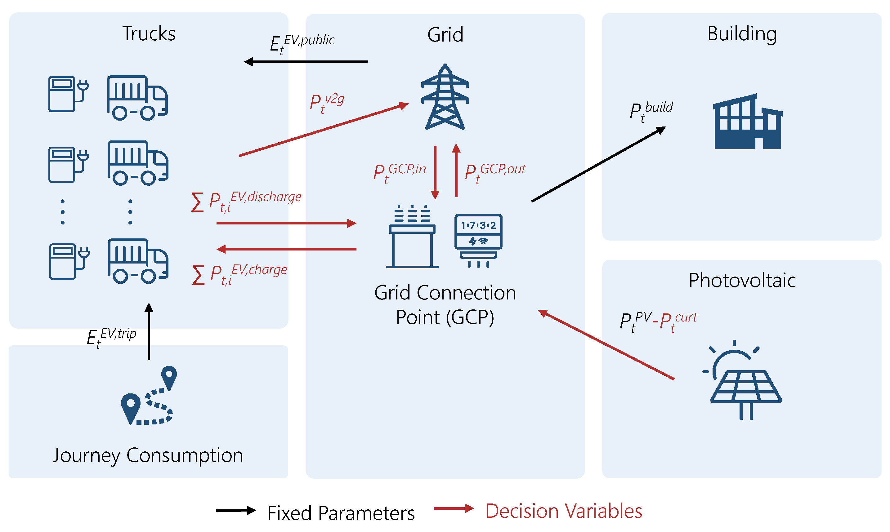
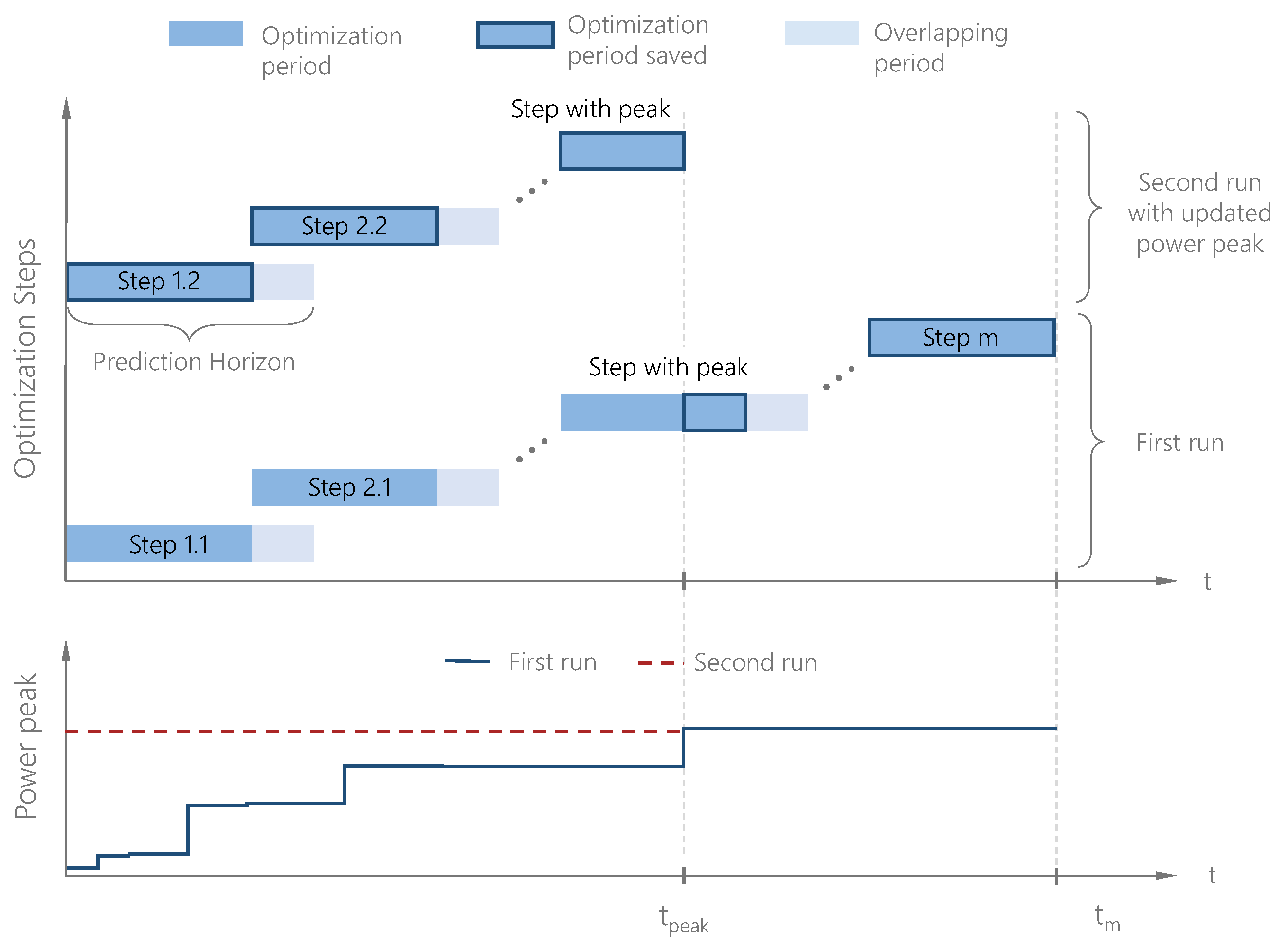
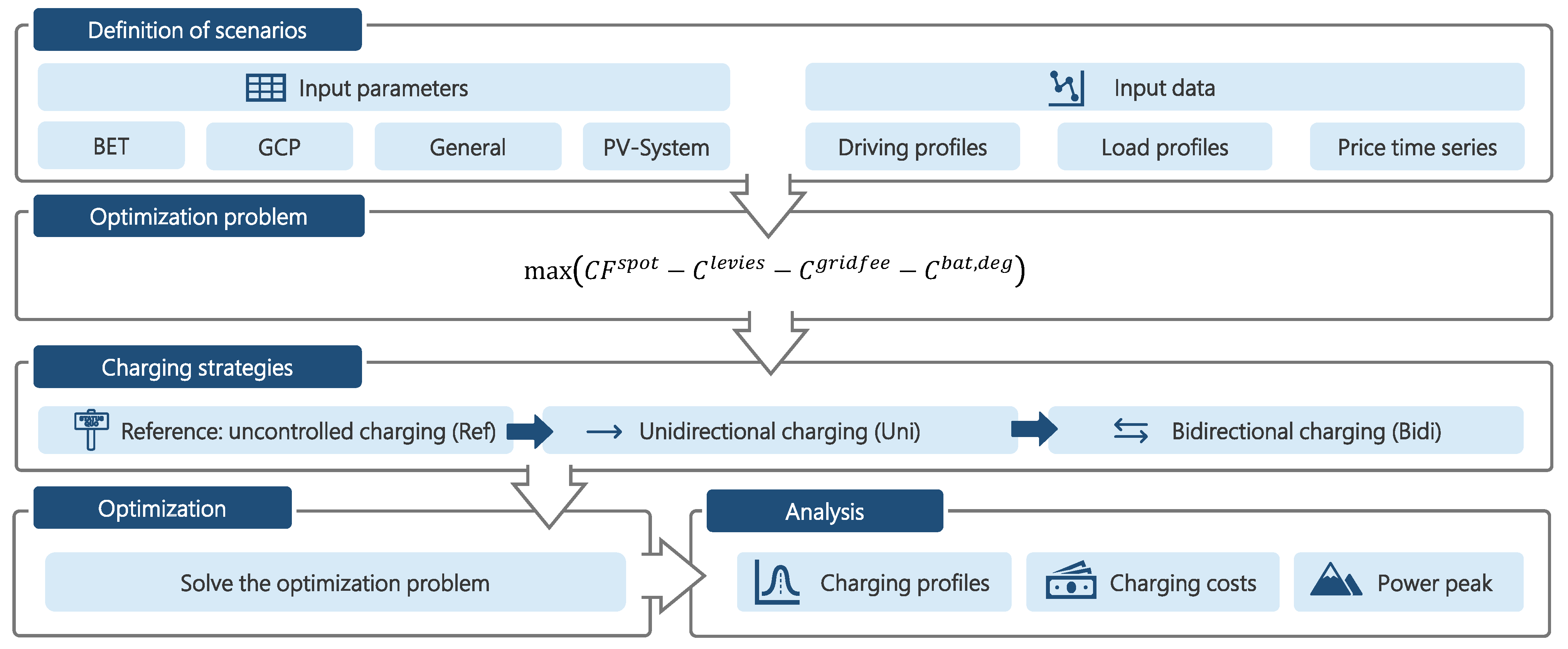
2.1. Optimization Model

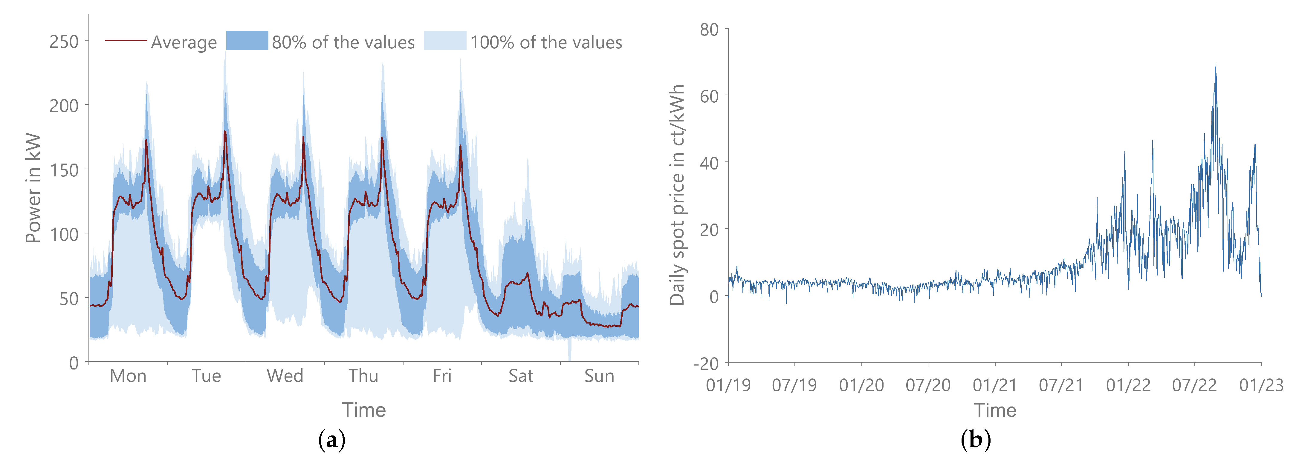
The optimization model eFlame was primarily developed to optimize several use cases for bidirectional charging separately. In [14,26], the use cases arbitrage trading and self-consumption optimization are elaborated upon. The use case peak shaving is dealt with in [7]. The novelty of the present paper is the combination of the use cases in the context of a multi-use optimization that was not implemented before. Figure 1 shows all power flows relevant to the optimization. At this point, we describe the optimization problem covering decision variables, objective function, and constraints. Linear optimization is a method that can be used to solve problems where the objective function and constraints are linear functions of the decision variables. The constraints can be formulated as equalities or inequalities. A mixed-integer linear program (MILP) problem includes integer decision variables. A comprehensive introduction to linear optimization is given in [27]. Since the model was primarily developed for optimizing battery-electric cars, the vehicles are generally referred to as EVs in the following model description.

For all decision variables, the non-negativity constraint applies. The constraint is exemplarily defined in Equation (1) for the received power $P_t^{GCP,in}$, and the feed-in power $P_t^{GCP,out}$ at the Grid Connection Point (GCP), but it can be applied to the remaining decision variables. The total number of time steps t in the observation horizon is represented by n.

$$P_t^{GCP,in}⩾0,P_t^{GCP,out}⩾0\forall t\in T=\left\{1,...,n\right\}$$

(1)

The photovoltaic (PV) generation is not a decision variable, but it may be influenced during the optimization via the curtailment $P_t^{curt}$. With this optimization variable, the generation of the PV system can be reduced, e.g., to prevent feed-in at negative prices. Using the decision variable $P_t^{GCP,peak}$, the maximum power at the grid connection point is determined. The charging power $P_t^{charge}$ and discharging power $P_t^{discharge}$ and the energy capacity of the battery $E_t^{EV}$ are further decision variables that are related to the EVs. Furthermore, there is the decision variable $P_t^{v2g}$, which is used to observe how much energy from the vehicles is fed back into the grid. The remaining decision variables $b_t^{charge}$, $b_t^{discharge}$, $b_t^{out}$, and $b_t^{in}$ are boolean variables, which are used to ensure that the power flow exchanges with the vehicles and the grid connection point are only in one direction at any time instant.

The objective of the optimization model is to maximize the revenue. The established objective function shown in Equation (2) consists of four terms: the cashflow from arbitrage trading at the spotmarket ${\mathit{CF}}^{spot}$, costs through levies $C^{levies}$, costs through grid fees $C^{gridfee}$, and a term that evaluates the opportunity costs due to battery degradation $C^{bat,deg}$. The different terms are defined in the following.

$$\begin{array}{c}max\left({\mathit{CF}}^{spot}-C^{levies}-C^{gridfee}-C^{bat,deg}\right)\end{array}$$

(2)

The cash flow, the difference between cash in- and outflows, from arbitrage trading at the spot market $C{F}^{spot}$ is calculated in Equation (3). Different market data can be selected for the price time series $p_t^{in}$ and $p_t^{out}$, but constant values may also be used.

$${\mathit{CF}}^{spot}=\sum _{t=1}^n\left({P_t}^{GCP,in}·p_t^{in}·\Delta t-{P_t}^{GCP,out}·p_t^{out}·\Delta t\right)\forall t\in T$$

(3)

Consumers have to pay a gridfee $C^{gridfee}$ to the Distibution System Operator (DSO) for the use of the grid infrastructure. In Germany, the grid fee for commercial customers is divided into a usage price $p^{usage}$ and a capacity price $p^{cap}$. The usage price depends on the energy consumed, whereas the capacity price depends on the annual peak power. The grid fee is included in the objective function of Equation (4).

$$C^{gridfee}=\sum _{t=1}^n{P_t}^{\mathit{GCP},in}·p^{usage}·\Delta t+P_{t=n}^{\mathit{GCP},peak}·p^{cap}\forall t\in T$$

(4)

Additionally, various taxes and levies are charged on electricity, and those are summarized through $C^{levies}$ and shown in Equation (5). Stationary battery storage may be partially exempt from levies, and such an exemption is also being discussed for bidirectional vehicles. The problem is to determine how much energy is actually fed back into the grid. This is especially problematic in combination with PV systems. Via the subtrahend of Equation (5), a partial exemption from the levies on energy fed back into the grid is implemented. The decision variable $P_t^{v2g}$ represents the power the vehicles feed into the grid and is introduced later in (17) and (18). It is an auxiliary variable calculated from the other power variables and is therefore not directly included in the power balance following in Equation (7). A partial exemption may be dynamically parameterized via the levies on V2G $p^{levies,v2g}$ that are still charged even if the energy is fed back into the grid. If $p^{levies,v2g}$ is set equal to $p^{levies}$, no exemption occurs. A full exemption can be achieved by setting $p^{levies,v2g}$ equal to zero.

$$\begin{array}{c}{\displaystyle C^{levies}=\sum _{t=1}^n{P_t}^{\mathit{GCP},in}·p^{levies}·\Delta t-\sum _{t=1}^n{P_t}^{v2g}·\left(p^{levies}-p^{levies,v2g}\right)·\Delta t\forall t\in T}\end{array}$$

(5)

The opportunity costs from battery degradation $C_{bat,deg}$ are included in the optimization problem by using Equation (6) based on [28]. The calculation of the degradation costs $C_{bat,deg}$ is based on the use of the battery and determined by the decrease of the available capacity $C^{loss}$ from a cycling aging model. The costs result primarily from the total charge quantity throughput, which is defined by the charging and discharging power. The price of the battery is represented by $c_{bat,buy}$, and $E^{EV,max}$ is the capacity of the battery. The used model assumes the end of life of the battery at a loss of 20% of the initial capacity.

$$\begin{array}{c}{C}_{bat,deg}=\frac{c_{bat,buy}·E^{EV,max}}{20\%}{C}_{loss}(P_t^{EV,charge},P_t^{EV,discharge})\forall t\in T\end{array}$$

(6)

The optimization model is restricted by several constraints concerning the GCP and the EVs. We start by introducing the boundary conditions of the GCP. According to the law of conservation of energy, the incoming power flows at the GCP must be equal to the outgoing power flows. This is ensured by Equation (7). The load profile of the building $P_t^{build}$ is integrated into the optimization as a static time series.

$$\begin{array}{c}{\displaystyle P_t^{\mathit{GCP},in}+\sum _{i=1}^{n_{EV}}{P}_t^{EV,discharge}+P_t^{PV}=}\\ {\displaystyle P_t^{\mathit{GCP},out}+\sum _{i=1}^{n_{EV}}{P}_t^{EV,charge}+P_t^{curt}+P_t^{build}\forall t\in T}\end{array}$$

(7)

For the determination of the grid fee $C^{gridfee}$ in Equation (4), the annual peak power at the GCP $P_t^{\mathit{GCP},peak}$ is required. Using Equation (8), the power peak is updated continuously during the optimization. Thus, the last time step n contains the annual power peak.

$$P_t^{\mathit{GCP},peak}⩾P_t^{\mathit{GCP},in},P_t^{\mathit{GCP},peak}⩾P_{t-1}^{\mathit{GCP},peak}\forall t\in T$$

(8)

Equations (9) and (10) are introduced to prevent energy from being purchased and fed in simultaneously at the GCP. In consequence, the boolean decision variables $b_t^{in}$ and $b_t^{out}$ are used. $P^{\mathit{GCP},max}$ describes the maximum grid connection capacity, which results from the transformer and structural conditions at the grid connection point. The combination of Equations (8) and (9) ensures the grid connection capacity $P^{\mathit{GCP},max}$ is always greater than or equal to the annual power peak $P_t^{\mathit{GCP},peak}$.

$$\begin{array}{c}{P}^{\mathit{GCP},max}·b_t^{in}⩾P_t^{\mathit{GCP},in},P^{GCP,max}·b_t^{out}⩾P_t^{\mathit{GCP},out}\forall t\in T\end{array}$$

(9)

$$\begin{array}{c}{b}_t^{out}+b_t^{in}⩽1\forall t\in T\end{array}$$

(10)

The following constraints are related to the EVs and apply separately for each EV. The energy balance of the vehicle battery must be maintained to preserve the physical consistency of the EVs. The energy stored in the EV battery in the first time step is defined by the constraint Equation (11). For the first time step, this equation defines the stored energy as equal to the initial stored energy plus the charged energy at the GCP minus the discharged energy and the energy consumed during trips $E_t^{EV,trip}$ plus the energy charged at public stations $E_{t=1}^{EV,public}$. Constant efficiencies for charging ${\eta }^{EV,charge}$ and discharging ${\eta }^{EV,discharge}$ are considered.

$$\begin{array}{c}{E}_{t=1}^{EV}={SOC}_{t=1}^{EV}·E^{EV,max}+P_{t=1}^{EV,charge}·{\eta }^{EV,charge}·\Delta t\\ -P_{t=1}^{EV,discharge}·{\eta }^{EV,discharge}·\Delta t-E_{t=1}^{EV,trip}+E_{t=1}^{EV,public}\end{array}$$

(11)

For the remaining time steps, Equation (12) applies, where the initially stored energy is replaced by the stored energy of the previous time step.

$$\begin{array}{c}{E}_t^{EV}=E_{t-1}^{EV}+P_t^{EV,charge}·{\eta }^{EV,charge}·\Delta t\\ -P_t^{EV,discharge}·{\eta }^{EV,discharge}·\Delta t-E_t^{EV,trip}+E_t^{EV,public}\forall t\in \left\{2,...,n\right\}\end{array}$$

(12)

Equation (13) ensures that the vehicles are always charged with a minimum State of Charge ${SOC}^{EV,dep,min}$ at departure. The condition is only valid for the time steps in which a vehicle departs, as indicated by the boolean variable $b_t^{EV,dep}$. This variable is determined before the optimization based on the driving profiles and is only equal to one if the vehicle departs. To ensure that the condition can also be met if the vehicle is only plugged in for a short time and thus the minimum SOC cannot be reached, a buffer $E_t^{buffer}$ is integrated into the condition. This buffer is also determined before the optimization.

$$\begin{array}{c}{E}_t^{EV}+E_t^{buffer}={SOC}^{EV,dep,min}·E^{EV,max}·b_t^{EV,dep}\forall t\in T\end{array}$$

(13)

Apart from public charging, each EV can only be charged or discharged if it is connected to a charging point at the GCP, and this is ensured by Equations (14) and (15). The boolean variable $b_t^{EV}$ is determined before the optimization based on the driving profiles. If the vehicle is plugged in, the variable is one, and otherwise it is zero. We assume that each vehicle has its own charging point. To prevent the EVs from charging and discharging at the same time, the decision variables $b_t^{charge}$ and $b_t^{discharge}$ are added to Equations (14) and (15). Equation (16) prevents both variables from being equal to one simultaneously. If only unidirectional charging is considered, the Equations (15) and (16) are omitted, and $P_t^{EV,discharge}$ is set to zero via a further boundary condition.

$$b_t^{EV}·b_t^{charge}·P^{EV,charge,max}⩾P_t^{EV,charge}\forall t\in T$$

(14)

$$b_t^{EV}·b_t^{discharge}·P^{EV,discharge,max}⩾P_t^{EV,discharge}\forall t\in T$$

(15)

$$\begin{array}{c}{b}_t^{charge}+b_t^{discharge}⩽1\forall t\in T\end{array}$$

(16)

Finally, boundary conditions are required to determine the power fed back from the EVs into the grid $P_t^{v2g}$. This variable is necessary to calculate the exemption from levies in Equation (5). Therefore, we choose a power balance based approach and rearrange Equation (7) according to the discharged energy. Since power can only be fed into the grid if no energy is purchased, $P_t^{\mathit{GCP},in}$ is set to zero. The discharged power is replaced by the introduced decision variable $P_t^{v2g}$, resulting in Equation (17). The boundary condition in Equation (18) ensures that $P_t^{v2g}$ cannot become greater than the feed-in power.

$$\begin{array}{c}{\displaystyle P_t^{v2g}⩽P_t^{\mathit{GCP},out}-P_t^{PV}+P_t^{curt}+P_t^{build}+\sum _{i=1}^{n_{EV}}{P}_t^{EV,charge}\forall t\in T}\end{array}$$

(17)

$$\begin{array}{c}{P}_t^{v2g}⩽P_t^{GCP,out}\forall t\in T\end{array}$$

(18)

Since the model is intended to examine entire years and since the use of boolean variables makes it a mixed-integer optimization problem, the computational effort required to solve the problem is rather high. In order to be able to solve it with a reasonable computational effort, the model is computed as a rolling optimization. The determination of the annual power peak is a special aspect of the rolling optimization, which will be explained in the following using the schematic diagram in Figure 2. For rolling optimization, the whole optimization period is divided into m smaller optimization time periods of uniform size. In individual optimization steps, each of the smaller optimization periods is optimized one after the other. The results of an optimization step are passed as start values to the next step. By using an overlapping period, we increase the prediction horizon for the optimization. After the m-th step, the first run of the optimization is finished. According to Equation (8), the power peak is continuously updated as shown in Figure 2 below. As can be seen in the figure, the first optimization steps are limited by a lower power peak compared to the later steps. Therefore, in a second optimization run, the affected steps before the occurrence of the annual power peak are optimized again with the updated power peak.

The sequence of the used optimization model eFlame is illustrated schematically in Figure 3. After importing the input parameters and input data described below, the optimization problem is set up. The optimization problem is solved sequentially considering the charging strategies: uncontrolled charging (ref), unidirectional charging (uni), and bidirectional charging (bidi). The results are examined separately for each charging strategy.

2.2. Input Data

As mentioned in Section 1, prior research on the topic of BETs has relied on assumptions regarding driving profiles. In this paper, we had the opportunity to use real-life data from a depot of a freight forwarding company in Germany. The company primarily operates in the short-haul segment. The data were provided within the framework of the project NEFTON in which partners from industry and science jointly develop a Megawatt Charging System (MCS) for BETs. Mobility data of the company’s trucks, historical load profiles of its buildings, and information about the PV system are included in the data. The selected depot can serve as a real-life example.

In the project NEFTON, driving data from several fleets of German fleet operators were recorded using high-resolution GPS data loggers. The recorded dataset includes 1.26 million km of driving data and is openly available in anonymized form in [29]. Only the driving data of the depot under consideration were extracted from this dataset. Since the data were recorded for trucks using diesel fuel, our investigation builds on the observation that the company desires to keep its services in the same way with electric trucks. The data are available for different lengths of time and were extended to uniform periods using a Markov process. To avoid oversizing the vehicle batteries, the missions in the dataset are divided into two clusters depending on the distance traveled. Missions with a distance of more than 200 km are grouped into the cluster regional transport and those with less than 200 km into the cluster local transport, which is similar to the classification of [30]. The annual driving profiles are taken as given and are presented in the following. Figure 4 shows the average percentage of vehicles in different locations for the two clusters. It can be seen that especially the mobility profiles from the Local Transport cluster have very high idle times at the depot and that at least 50% of the BETs are always present at the depot. On weekends and at night, most of the vehicles are located at the depot. The driving profiles of the cluster Regional Transport show significantly lower idle times at the depot. During daytime on weekdays, 80% of the vehicles are absent. On weekends, almost 40% are not at the depot. In addition, the driving profiles of the Regional Transport cluster show high parking durations in industrial areas and other locations. The difference between the two clusters is also evident from the characteristic values included in

Table 1. Characteristics of the used driving profiles.

Characteristics	Local Transport	Regional Transport
Daily kilometrage (Weekdays/Weekends)	53.8 km/0.75 km	250 km/4.2 km
Percentage at depot (Weekdays/Weekends)	78.20%/95.19%	37.80%/63.40%
Annual kilometrage	14.382 km	65.750 km
Average consumption per km	1.1 kWh/km	1.26 kWh/km
Annual energy consumption	14.9 MWh	83.4 MWh

. The annual kilometrage of the Local Transport cluster is about 14,000 km. This is significantly lower than the kilometrage of the Regional Transport cluster of about 66,000 km. The electrical energy consumption for the driving profiles is determined using the model from [31]. The average annual consumption determined in this way is also included in Table 1. The variables $b_t^{EV,dep}$, $E_t^{buffer}$, $b_t^{EV}$, $E_t^{EV,trip}$ and $E_t^{EV,public}$ are determined based on the driving profiles and serve as inputs for the optimization model.

In addition to the driving profiles, the load profile of the building of the depot $P_t^{build}$ is another important input for the optimization. The used load profile shown in Figure 5b for an average week relies on real data of the depot. From the annual time series, the average was determined for each quarter-hour of the week as well as the ranges in which 80% and 100% of the values lie. The plot shows that there are significant load peaks in the evening hours on weekdays, indicating suitability for peak shaving. The load is significantly lower at weekends and at night than it is during the day on weekdays.

We assume that the depot pays variable electricity prices based on the prices of the electricity exchange. Therefore, we used the intraday auction prices as electricity prices $p_t^{in}$ and $p_t^{out}$ for the optimization. In Europe, there are various short-term markets on the power exchange. One of those markets is the intraday auction. Due to the shorter time slices of quarter hours compared to the day-ahead market, in which hourly products are traded, this market offers higher price spreads. Thus, the revenue opportunities for flexibilities like bidirectional EVs are increased. The development of the prices of the intraday auction from the beginning of 2019 to the end of 2022 is shown in Figure 5a. As a consequence of the energy crisis, the price has risen from around 4 ct/kWh to a maximum of over 70 ct/kWh, and also the price spreads increased significantly.

The PV generation is determined as a time series depending on the historical irradiation data on CAMS level as a function of the orientation of the PV plant and its peak power [32]. The irradiation data are used for the location of the depot for the weather year 2012. The weather year is chosen based on the recommendation in [33].

2.3. Input Parameters

After introducing the data source and the model in the previous sections, the input parameters are presented in the following. For this purpose, we define a base scenario for which the input parameters are listed in

Table 2. Parameters of the base scenario and sensitivities.

Category	Parameter	Symbol	Unit	Value	Sensitivities
General	Year			2021	2019, 2020, 2022
	Time step size	t	h	0.25
	Optimization period		h	168
	Overlapping period		h	24
GCP	Levies on V2G	$p^{levies,v2g}$	EUR/kWh	$p^{levies}$	0.02, 0
	Price for public charging	$p^{public}$	EUR/kWh	0.50
	Max. grid connection capacity	$P^{\mathit{GCP},max}$	MW	5	0.7, 1, 1.5, 2
	Feed-in remuneration PV (ref)		EUR/kWh	0.06
BETs	Number of vehicles	$n_{EV}$		30	20, 40, 50
	Efficiency of charging	${\eta }^{EV,charge}$		0.926
	Efficiency of discharging	${\eta }^{EV,discharge}$		0.921
	Capacity of vehicle battery	$E^{EV,max}$	kWh	250/500
	Minimum SOC at departure	${SOC}^{EV,dep,min}$		1
	Maximum charging/ discharging power	$P^{EV,max}$	kW	100	50, 200, 300
	Price of battery	$c_{bat,buy}$	EUR/kWh	139
PV system	Peak power		kW	1000	0, 2000
	Azimuth angle		°	0
	Tilt angle		°	35

. By varying different parameters of this base scenario, various sensitivities are examined. For the sensitivity analysis, one parameter of the base scenario is changed, while the rest of the parameters are left unchanged. The varied parameters of the sensitivity analysis are also included in the table. The base year is 2021, and the optimization is performed at a time step size of 15 min. As Figure 2 illustrates, we use a rolling approach and divide the examined years into 61 optimization steps. The observation period of each step is seven days, consisting of the optimization period of six days and one day of overlap. In contrast to real-world charging management systems that apply forecasts, we assume perfect foresight for each optimization step. In the base scenario, no exemption of levies on energy fed back into the grid is assumed. Therefore, $p^{levies}$ is set to be equal to $p^{levies,v2g}$. However, the exemption is considered in the sensitivity analysis. In the base scenario, no limitation of the grid connection capacity is considered. Thus, $P^{\mathit{GCP},max}$ is set to the oversized value of 5 MW. A limitation of $P^{\mathit{GCP},max}$ is examined in the sensitivity analysis. The grid connection capacity is minimally limited to 700 kW, since a lower capacity would result in the curtailment of the PV system in times of high irradiation. The feed-in tariff of 0.06 EUR/kWh is an assumed value suitable for Germany and is only used in the reference simulation as $p_t^{out}$. It is also assumed that 30 BETs of the depot are electrified. The number of electric vehicles is one of the sensitivities examined. According to the distribution from the dataset, 30% of the vehicles are used for regional traffic and 70% are used for local traffic. The appropriate driving profiles are divided among the BETs according to the distribution, and a battery capacity of 250 kWh for local and 500 kWh for regional traffic is assumed. Based on [34], the price of the vehicle battery $c_{bat,buy}$ is set to 139 EUR/kWh. The parameters of the PV system are selected according to the system of the real depot.

In addition to the year 2021 of the base scenario, the years 2019, 2020, and 2022 are also examined. For the optimization of the different years, several parameters have to be varied. In contrast, only one parameter is changed at a time in the sensitivity analysis presented below. The other parameters remain unchanged. In consequence, these year-dependent parameters are separated in

Table 3. Year-dependent parameters.

Year	${\mathit{p}}_{\mathit{t}}^{\mathbf{ref}}$ (EUR/kWh)	${\mathit{p}}^{\mathit{levies}}$ (EUR/kWh)	${\mathit{p}}_{\mathbf{usage}}$ (EUR/kWh)	${\mathit{p}}_{\mathbf{cap}}$ (EUR/kW)
2019	0.038	0.131	0.047	16.37
2020	0.030	0.135	0.052	18.36
2021	0.097	0.133	0.054	18.65
2022	0.245	0.495	0.056	19.20

. For the reference simulation, a constant price based on the average day-ahead price is assumed for $p_t^{in}$ [35]. For the levies, the real historical values for Germany from [36] are used. The prices for the grid fees are also based on historical values of the grid operator Netze BW, where the depot under consideration is located [37]. We use the prices for medium voltage networks and consider an annual usage time of less than 2500 h.

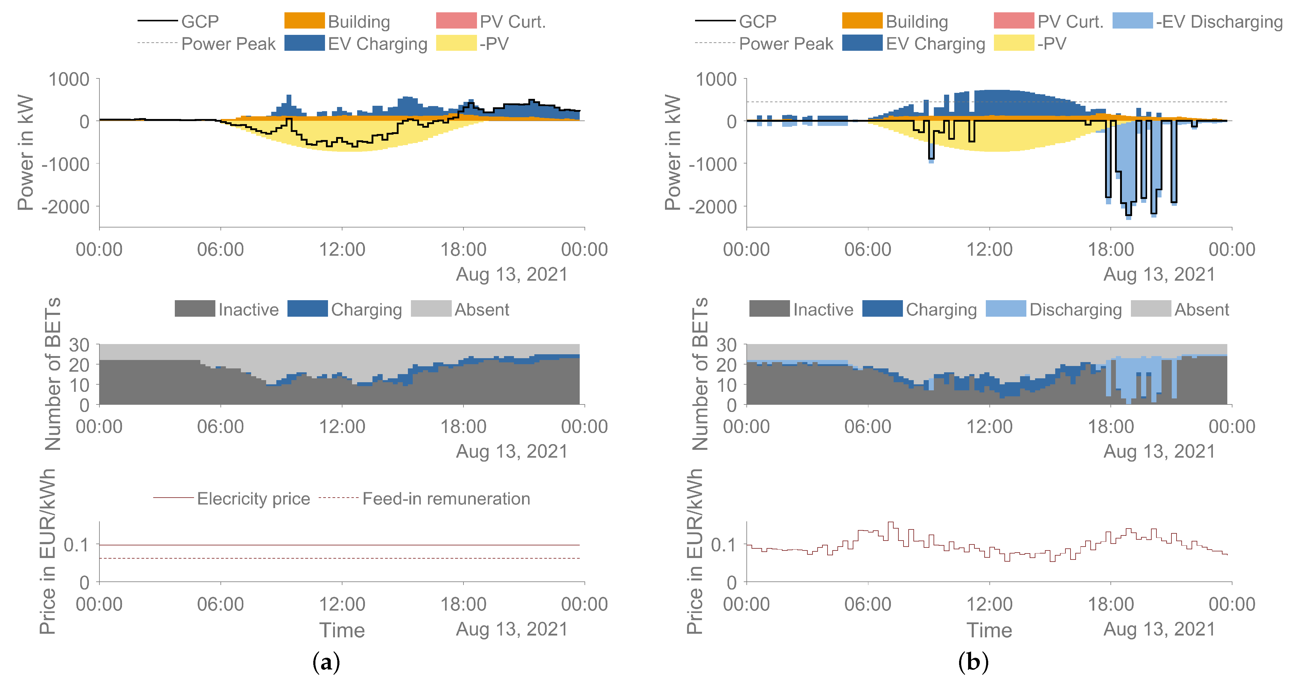
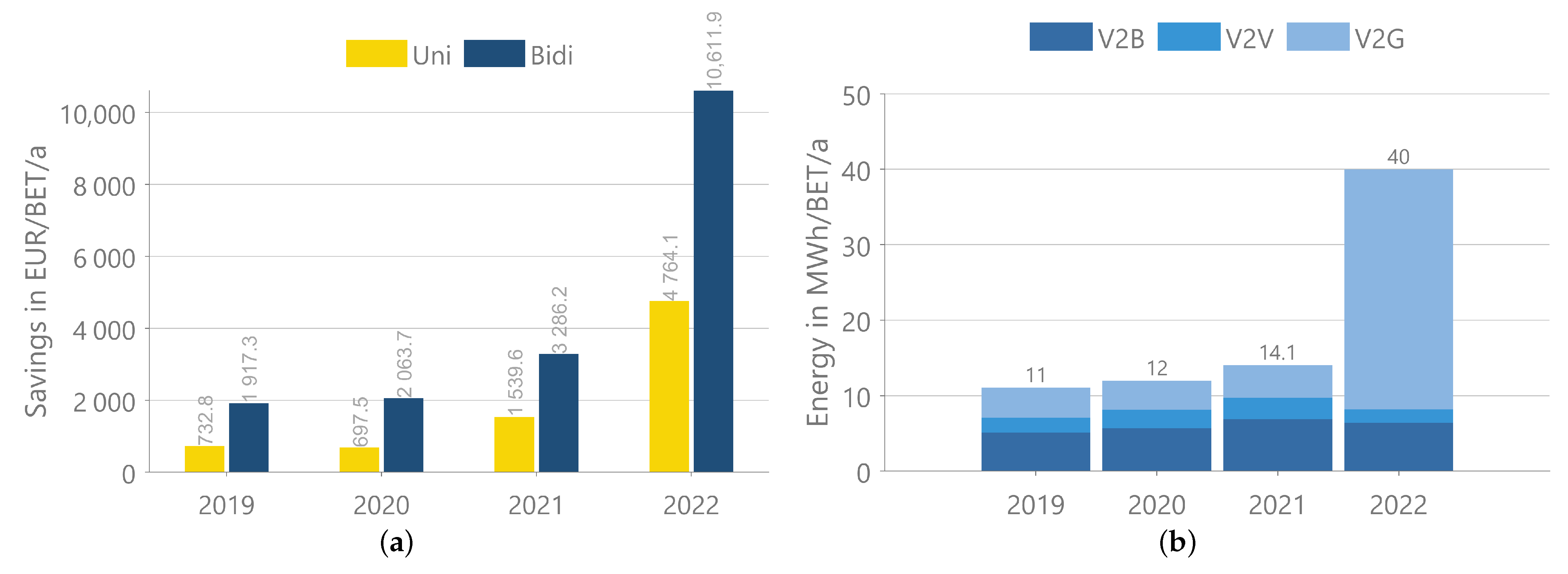
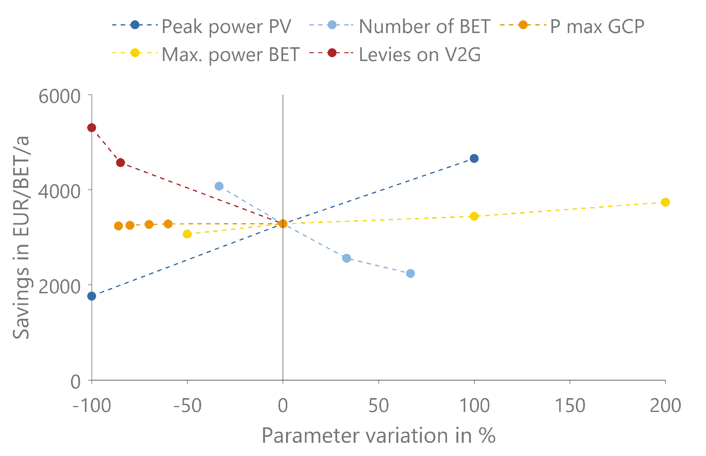
3. Results and Discussion

In order to better understand the results presented in the following, we first look at a single example day. A sunny weekday in August from the base scenario in 2021 is chosen. Figure 6 is intended to explain the charging strategies and shows the important time series from the optimization results for the example day. The results for the reference with uncontrolled charging are shown on the left, and those for bidirectional charging are shown on the right. In the upper diagram, the power of the different components is plotted as a stacked area diagram. The resulting power at the grid connection point $P_t^{\mathit{GCP}}=P_t^{\mathit{GCP},\mathit{in}}+P_t^{\mathit{GCP},\mathit{out}}$ is shown as a black line. The center diagram illustrates for each time step how many vehicles are attendant and how many of them are charging or discharging. The given prizes are shown in the lower diagram. Levies and grid fees are not included in the prices.

With uncontrolled reference charging, the vehicles are charged immediately when they arrive at the depot. Even though some vehicles arrive and charge at midday, this leads to charging processes in the evening and at night where the power of the PV system is unavailable. The unused energy from the PV system is fed into the grid for the low feed-in tariff, and more expensive energy is purchased from the grid in the evening hours. The situation is different with the bidirectional charging strategy. According to the optimization problem presented in Section 2.1, the objective of the optimization is to maximize the revenue. One way to achieve this is to shift the charging process to times when PV power is available, since this power is not priced in the optimization problem. This shifting is clearly visible in the diagram because the area of the BET charging matches the PV generation. Energy can also be fed into the grid to maximize the revenue. Such a feed-in takes place on the example day from around 6 PM, when many vehicles are available and high energy prices are reached. Due to the oversized grid connection capacity of 5 MW, a large number of BETs discharge at the same time, resulting in a high feed-in power of over 2 MW. Because of the power price integrated in Equation (8), the annual power peak of the reference of 1.3 MW is lowered in the optimization to 0.4 MW. The power price only affects the purchased power, which allows the feed-in with a higher power. Figure 6 also clearly shows that outside the times with PV generation, the vehicles supply each other and also the building with energy.

The results of the base scenario are compared with those of the other examined years in Figure 7. Figure 7a shows the annual savings for the optimization with unidirectional (uni) and bidirectional (bidi) BETs. The savings are calculated from the difference between the costs in the reference simulation and the respective charging strategy and are normalized per vehicle. Before 2021, the savings are modest at about 2000 EUR/BET even with bidirectional vehicles. As energy prices rise from 2021 (cf. Figure 5), savings also increase significantly. Thus, almost 3300 EUR/BET can be achieved in 2021 with the bidirectional and 1500 EUR with the unidirectional charging strategy. In 2022, the savings skyrocket up to more than 10,000 EUR/BET. On the one hand, this can be explained by the fact that the reference costs in 2021 and 2022 rise due to the higher prices. On the other hand, the increasing price spreads and falling levies are responsible for the high savings, as this makes arbitrage trading significantly more attractive. In comparison, the authors of [13] estimate lower savings of 1515 EUR/BET. The deviation mainly results from the simplified price time series they use, which does not adequately reflect realistic price spreads of the spot market.

A corresponding observation can be made in Figure 7b, where the average discharged energy per BET and year is illustrated. It only represents the results from the bidirectional charging strategy, because only here can discharging occur. The diagram contains information on how much energy is fed back to the building (V2B), to other vehicles (V2V), or to the grid (V2G). Discharging into the grid takes place in order to generate revenues. V2G dominates the discharged energy in 2022. This explains the high revenues discussed above. Since the load of the building cannot flexibly respond to prices and PV generation, the BETs can, through discharging, supply the building with cheaper energy from the PV system or the grid in time steps with high electricity prices. Furthermore, V2B can serve to reduce the annual power peak. The same applies for V2V, where vehicles with high parking duration can supply frequently driving vehicles with cheap energy. V2V is thus another way to reduce charging cost. The share of V2B is relatively similar in all years and is slightly higher in 2021 and 2022 than in previous years. V2V takes the smallest share of the discharged energy in all years. In the reference scenario, the self-consumption rate is around 50% in all the examined years. The optimization increases this ratio to almost 65% with unidirectional BETs and 95% with bidirectional BETs.

To examine the influence of individual parameters on the results, the results of the sensitivity analysis for the bidirectional charging strategy are shown in Figure 8. In the sensitivity analysis, we varied various parameters that could impact the savings. Depending on the results, the values of these sensitivity parameters are selected iteratively. The diagram shows the percentage deviation of the sensitivity parameters from the parameters of the base scenario on the x-axis and the annual savings on the y-axis. The absolute values of the sensitivity parameters are provided in the last column of Table 2. The point in the diagram where the parameter variation is zero contains the savings of the base scenario already shown in Figure 7 (2021). The reduction of the grid connection capacity $P^{\mathit{GCP},max}$ has the least impact on the savings. With the limitation of 700 kW (parameter variation = 86%), the grid connection capacity is still large enough and the savings decrease only minimally. A reduction of $P^{\mathit{GCP},max}$ below 700 kW would reduce the savings more significantly, but then the PV system (1 MW peak) has to be curtailed. More points are calculated for this parameter to determine the boundary where no curtailment occurs. The savings decrease without a PV system but increase with a larger PV system. With higher charging and discharging power, savings can be increased. In the analysis, the charging power of 300 kW (parameter variation = 200%) leads to increased savings above 3700 EUR per BET. A larger number of vehicles reduces the savings per vehicle. The parameter with the strongest impact on the savings is the levies on the energy fed back. In the base scenario, we assume the worst case for V2G without any exemption from levies for energy fed back into the grid. Therefore, $p^{levies,v2g}$ is set equal to $p^{levies}$. With full exemption ($p^{levies,v2g}=0$), the annual savings per BET strongly increase to 5300 EUR. However, these savings are only possible with a significantly higher, discharged energy from the BETs to the grid.

4. Conclusions and Outlook

This study presents a model to optimize charging processes in depots for EVs. In addition to the chargers, the depots may be equipped with a PV system and an inflexible load, e.g., from a building. The objective of the optimization is to minimize the charging cost. The cost reduction is achieved by increasing the self-consumption rate, reducing the annual peak load, shifting charging processes to time steps with low energy prices, and arbitrage trading. Through this combination of different use cases, a multi-use optimization is implemented. The optimization is implemented on a rolling basis. Despite a higher computing effort, even large depots with hundreds of vehicles can be optimized using this method. The economic benefits of V2G can be compromised by levies on purchased energy fed back into the grid. A full or partial exemption from levies for bidirectional EVs could solve this problem in the future. The implementation of this exemption is difficult, as it may only apply to the energy fed back into the grid. Energy consumed while driving must be taxed. If EVs feed into the grid and are charged by energy from the grid plus a PV system, then no exemption may apply to fed-in energy provided by the PV system. A partial exemption from levies is therefore implemented in the presented model. The amount of the exemption from levies can be chosen freely, and the approach even works with PV systems.

The model presented is used to optimize a depot for BETs. The study shows that the examined depot is very well suited for implementing bidirectional charging strategies. The operator of the depot can benefit monetarily from it. Due to the large PV system and the long duration of attendance of the BETs, the depot under consideration offers excellent conditions for optimization. In the base scenario, the bidirectional charging strategy can save 3300 EUR per vehicle and year compared to uncontrolled charging. A self-consumption rate of 95% can be achieved and the peak load can be significantly reduced. Arbitrage trading is only worthwhile when price spreads are high like in the examined years 2021 and 2022. Levies on fed-back energy impede arbitrage trading. According to the results of the sensitivity analysis, the exemption from levies can significantly increase savings. We examined the exemption from levies within a sensitivity analysis. At least a partial exemption from levies would be a precondition for the successful operation of V2G.

For further research, we propose a three-step strategy: Firstly, the model can be readily adapted to include additional use cases, e.g., providing frequency control. Secondly, instead of solely decreasing charging costs, it could be further developed to minimize the total cost of ownership (TCO) of the depot. Thirdly, the method can be applied to examine other depots by simply exchanging the database. The model is not limited to depots for BETs and can also be used to optimize depots for passenger cars or buses. This paper is therefore a basis for further research on the topic of bidirectional charging in depots for EVs.

References

1. Høj, J.; Juhl, L.; Lindegaard, S. V2G—An Economic Gamechanger in E-Mobility? WEVJ 2018, 9, 35. [Google Scholar] [CrossRef]
2. Kern, T.; Kigle, S. Modeling and evaluating bidirectionally chargeable electric vehicles in the future European energy system. Energy Rep. 2022, 8, 694–708. [Google Scholar] [CrossRef]
3. Nissan Approves First Bi-Directional Charger for Use With Nissan LEAF in the U.S. 2022. Available online: https://usa.nissannews.com/en-US/releases/nissan-approves-first-bi-directional-charger-for-use-with-nissan-leaf-in-the-us (accessed on 17 February 2024).
4. CO2 Emissions from Heavy-Duty Vehicles Preliminary CO2 Baseline (Q3–Q4 2019) Estimate. 2022. Available online: https://www.acea.auto/files/ACEA_preliminary_CO2_baseline_heavy-duty_vehicles.pdf (accessed on 17 February 2024).
5. New Commercial Vehicle Registrations: Vans +14.6%, Trucks +16.3%, Buses +19.4% in 2023. 2024. Available online: https://www.acea.auto/cv-registrations/new-commercial-vehicle-registrations-vans-14-6-trucks-16-3-buses-19-4-in-2023/ (accessed on 17 February 2024).
6. Earl, T.; Mathieu, L.; Cornelis, S.; Kenny, S.; Ambel, C.C.; Nix, J.C. Analysis of long haul battery electric trucks in EU Marketplace and technology, economic, environmental, and policy perspectives. In Proceedings of the 8th Commercial Vehicle Workshop, Graz, Austria, 17–18 May 2018. [Google Scholar]
7. Kern, T.; Bukhari, B. Peak Shaving—A cost-benefit analysis for different industries. In Proceedings of the 12. Internationale Energiewirtschaftstagung an der TU Wien, Wien, Austria, 8–10 September 2021. [Google Scholar]
8. Cunanan, C.; Tran, M.K.; Lee, Y.; Kwok, S.; Leung, V.; Fowler, M. A Review of Heavy-Duty Vehicle Powertrain Technologies: Diesel Engine Vehicles, Battery Electric Vehicles, and Hydrogen Fuel Cell Electric Vehicles. Clean Technol. 2021, 3, 474–489. [Google Scholar] [CrossRef]
9. Nykvist, B.; Olsson, O. The feasibility of heavy battery electric trucks. Joule 2021, 5, 901–913. [Google Scholar] [CrossRef]
10. Link, S.; Plötz, P. Technical Feasibility of Heavy-Duty Battery-Electric Trucks for Urban and Regional Delivery in Germany—A Real-World Case Study. WEVJ 2022, 13, 161. [Google Scholar] [CrossRef]
11. Liimatainen, H.; van Vliet, O.; Aplyn, D. The potential of electric trucks—An international commodity-level analysis. Appl. Energy 2019, 236, 804–814. [Google Scholar] [CrossRef]
12. Zähringer, M.; Wolff, S.; Schneider, J.; Balke, G.; Lienkamp, M. Time vs. Capacity—The Potential of Optimal Charging Stop Strategies for Battery Electric Trucks. Energies 2022, 15, 7137. [Google Scholar] [CrossRef]
13. Razi, R.; Hajar, K.; Hably, A.; Mehrasa, M.; Bacha, S.; Labonne, A. Assessment of predictive smart charging for electric trucks: A case study in fast private charging stations. In Proceedings of the 2022 IEEE International Conference on Electrical Sciences and Technologies in Maghreb (CISTEM), Tunis, Tunisia, 26–28 October 2022; pp. 1–6. [Google Scholar] [CrossRef]
14. Kern, T.; Dossow, P.; von Roon, S. Integrating Bidirectionally Chargeable Electric Vehicles into the Electricity Markets. Energies 2020, 13, 5812. [Google Scholar] [CrossRef]
15. Englberger, S.; Abo Gamra, K.; Tepe, B.; Schreiber, M.; Jossen, A.; Hesse, H. Electric vehicle multi-use: Optimizing multiple value streams using mobile storage systems in a vehicle-to-grid context. Appl. Energy 2021, 304, 117862. [Google Scholar] [CrossRef]
16. Roselli, C.; Sasso, M. Integration between electric vehicle charging and PV system to increase self-consumption of an office application. Energy Convers. Manag. 2016, 130, 130–140. [Google Scholar] [CrossRef]
17. Biedenbach, F.; Valerie, Z. Opportunity or Risk? Model-Based Optimization of Electric Vehicle Charging Costs for Different Types of Variable Tariffs and Regulatory Scenarios from a Consumer Perspective. In Proceedings of the CIRED Porto Workshop 2022: E-mobility and Power Distribution Systems, Porto, Portugal, 2–3 June 2022. [Google Scholar] [CrossRef]
18. Battke, B.; Schmidt, T.S. Cost-efficient demand-pull policies for multi-purpose technologies—The case of stationary electricity storage. Appl. Energy 2015, 155, 334–348. [Google Scholar] [CrossRef]
19. Parra, D.; Patel, M.K. The nature of combining energy storage applications for residential battery technology. Appl. Energy 2019, 239, 1343–1355. [Google Scholar] [CrossRef]
20. Jahic, A.; Eskander, M.; Schulz, D. Charging Schedule for Load Peak Minimization on Large-Scale Electric Bus Depots. Appl. Sci. 2019, 9, 1748. [Google Scholar] [CrossRef]
21. Duan, M.; Liao, F.; Qi, G.; Guan, W. Integrated optimization of electric bus scheduling and charging planning incorporating flexible charging and timetable shifting strategies. Transp. Res. Part C Emerg. Technol. 2023, 152, 104175. [Google Scholar] [CrossRef]
22. Verbrugge, B.; Rauf, A.M.; Rasool, H.; Abdel-Monem, M.; Geury, T.; El Baghdadi, M.; Hegazy, O. Real-Time Charging Scheduling and Optimization of Electric Buses in a Depot. Energies 2022, 15, 23. [Google Scholar] [CrossRef]
23. Houbbadi, A.; Trigui, R.; Pelissier, S.; Bouton, T.; Redondo-Iglesias, E. Multi-Objective Optimisation of the Management of Electric Bus Fleet Charging. In Proceedings of the 2017 IEEE Vehicle Power and Propulsion Conference (VPPC), Belfort, France, 11–14 December 2017; pp. 1–6. [Google Scholar] [CrossRef]
24. Raab, A.F.; Lauth, E.; Strunz, K.; Göhlich, D. Implementation Schemes for Electric Bus Fleets at Depots with Optimized Energy Procurements in Virtual Power Plant Operations. World Electr. Veh. J. 2019, 10, 5. [Google Scholar] [CrossRef]
25. Biedenbach, F.; Blume, Y. Size matters: Multi-use Optimization of a Depot for Battery Electric Heavy-Duty Trucks. In Proceedings of the EVS36, Sacramento, CA, USA, 11–14 June 2023. [Google Scholar]
26. Kern, T.; Dossow, P.; Morlock, E. Revenue opportunities by integrating combined vehicle-to-home and vehicle-to-grid applications in smart homes. Appl. Energy 2022, 307, 118187. [Google Scholar] [CrossRef]
27. Ploskas, N.; Samaras, N. Linear Programming Using MATLAB, 1st ed.; Springer International Publishing AG: Cham, Switzerland, 2017. [Google Scholar]
28. Preis, V.; Biedenbach, F. Assessing the incorporation of battery degradation in vehicle-to-grid optimization models. Energy Inform. 2023, 6, 33. [Google Scholar] [CrossRef]
29. Balke, G.; Adenaw, L. Heavy commercial vehicles’ mobility: Dataset of trucks’ anonymized recorded driving and operation (DT-CARGO). Data in Brief. 2023, 48, 109246. [Google Scholar] [CrossRef]
30. Borlaug, B.; Moniot, M.; Birky, A.; Alexander, M.; Muratori, M. Charging needs for electric semi-trailer trucks. Renew. Sustain. Energy Transit. 2022, 2, 100038. [Google Scholar] [CrossRef]
31. Sripad, S.; Viswanathan, V. Performance Metrics Required of Next-Generation Batteries to Make a Practical Electric Semi Truck. ACS Energy Lett. 2017, 2, 1669–1673. [Google Scholar] [CrossRef]
32. Schroedter-Homscheidt, M.; Hoyer-Klick, C.; Killius, N.; Lefèvre, M.; Wald, L.; Wey, E.; Saboret, L. User’s Guide to the CAMS Radiation Service—Status December 2017; ECMWF: Reading, UK, 2017. [Google Scholar]
33. Guminski, A.; Fiedler, C.; Kigle, S.; Pellinger, C.; Dossow, P.; Ganz, K.; Jetter, F.; Kern, T.; Limmer, T.; Murmann, A.; et al. eXtremOS Summary Report; Forschungsstelle für Energiewirtschaft e. V.: Munich, Germany, 2021. [Google Scholar] [CrossRef]
34. Veronika Henze. Lithium-Ion Battery Pack Prices Rise for First Time to an Average of $151/kWh. 2022. Available online: https://about.bnef.com/blog/lithium-ion-battery-pack-prices-rise-for-first-time-to-an-average-of-151-kwh/ (accessed on 17 February 2024).
35. EPEX-Spot SE. Market Data of EPEX-Spot SE; EPEX-Spot SE: Paris, France, 2023. [Google Scholar]
36. BDEW. BDEW Electricity Price Analysis Beginning of 2023. 2023. Available online: https://www.bdew.de/service/daten-und-grafiken/bdew-strompreisanalyse/ (accessed on 17 February 2024).
37. Netze BW GmbH. Prices for the Use of the Electricity Distribution Grid of Netze BW GmbH; Netze BW GmbH: Stuttgart, Germany, 2023. [Google Scholar]
Figure 1. Schematic representation of interrelations in the optimization model.
Wevj 15 00084 g001
Figure 2. Schematic diagram explaining the used rolling optimization process.
Wevj 15 00084 g002
Figure 3. Schematic diagram explaining the used methodology.
Wevj 15 00084 g003
Figure 4. Layered percentage of BETs at different locations over the week. (a) Local Transport cluster, (b) Regional Transport cluster.
Wevj 15 00084 g004
Figure 5. Visualization of input data: (a) electric load profile of the depot building, (b) daily average price intraday auction.
Wevj 15 00084 g005
Figure 6. Results for an example day for different charging strategies.: (a) reference, (b) bidirectional.
Wevj 15 00084 g006
Figure 7. Results of the analyzed years: (a) annual savings, (b) discharged energy.
Wevj 15 00084 g007
Figure 8. Results of the sensitivity analysis for the bidirectional charging strategy.
Wevj 15 00084 g008