Article

Joint Estimation of State of Charge and State of Health of Lithium-Ion Batteries Based on Stacking Machine Learning Algorithm

1
School of Materials Science and Chemical Engineering, Harbin University of Science and Technology, Harbin 150080, China
2
School of Electrical and Electronic Engineering, Harbin University of Science and Technology, Harbin 150080, China
*
Authors to whom correspondence should be addressed.
World Electr. Veh. J. 2024, 15(3), 75; https://doi.org/10.3390/wevj15030075
Submission received: 19 January 2024 / Revised: 7 February 2024 / Accepted: 14 February 2024 / Published: 20 February 2024
(This article belongs to the Special Issue Propulsion Systems of EVs 2.0)

Abstract

:
Conducting online estimation studies of the SOH of lithium-ion batteries is indispensable for extending the cycle life of energy storage batteries. Data-driven methods are efficient, accurate, and do not depend on accurate battery models, which is an important direction for battery state estimation research. However, the relationships between variables in lithium-ion battery datasets are mostly nonlinear, and a single data-driven algorithm is susceptible to a weak generalization ability affected by the dataset itself. Meanwhile, most of the related studies on battery health estimation are offline estimation, and the inability for online estimation is also a problem to be solved. In this study, an integrated learning method based on a stacking algorithm is proposed. In this study, the end voltage and discharge temperature were selected as the characteristics based on the sample data of NASA batteries, and the B0005 battery was used as the training set. After training on the dataset and parameter optimization using a Bayesian algorithm, the trained model was used to predict the SOH of B0007 and B0018 models. After comparative analysis, it was found that the prediction results obtained based on the proposed model not only have high accuracy and a short running time, but also have a strong generalization ability, which has a great potential to achieve online estimation.

1. Introduction

New, pollution-free renewable energy, represented by wind and solar energy, has difficulty generating electricity continuously and steadily. Energy storage is a crucial factor for renewable energy to become a fully reliable primary energy source [1]. With the characteristics of high energy density and high power density, lithium-ion batteries are widely used in energy storage systems. The battery state of charge is an important parameter to measure the performance of Li-ion batteries, while the SOH is a measure of a battery’s lifetime [2]. The development of online estimation studies of the SOC and SOH of lithium-ion batteries is essential to extend the cycle life of the batteries to reduce the potential for accidents.
Currently, there are three main methods for SOC estimation: the time integration method, the open-circuit voltage method, and the data-driven method. Among them, the time integration method discretely sums the current flowing through the battery and obtains the SOC value by simple division. The time integration method estimates the SOC by measuring current and time. Its advantage is simplicity and directness, without the need for additional sensors. However, due to measurement errors and integration drift, time integration methods may lead to cumulative errors in SOC estimation. The open-circuit voltage method measures the open-circuit voltage of the battery and obtains the charging state according to the corresponding relationship between the open-circuit voltage and the charging state. Its advantage is that it is non-invasive and does not require additional measuring equipment. Reference [3] proposed a fast and accurate method to measure the OCV after comparing three conversion methods of differential equations, thus improving the accuracy of SOC prediction. Reference [4] proposed a novel constant-current/constant-voltage charging control strategy for batteries by adjusting the battery charging current based on the estimation of the open-circuit voltage parameter. Reference [5] used the open-circuit voltage method to obtain an SOC estimate based on the average value calculated from the random forest output OCV-SOC curve to reduce the hysteresis effect. Wang et al. [6] proposed a new method for calculating model parameters and estimating the state of charge of lithium-ion batteries based on the parameter-estimated open-circuit voltage (OCV) under multi-temperature conditions. Although the accuracy is relatively high, the OCV method requires a long resting time to reach the equilibrium state in practical tests, and the resting time is affected by the environmental conditions and monitoring equipment, so it is usually used in laboratories or calibration-assisted techniques.
The data-driven method only needs to extract features using physical quantities measured during battery charging and discharging, and then uses these features to train a model to establish a mapping model between battery data features and the SOC. Reference [7] proposed a low-dimensional classification model based on machine learning and an equivalent circuit model, which can estimate the SOC with an accuracy of more than 93%. Reference [8] used 18 machine learning algorithms to predict the SOC and applied different filters to improve the estimator. The Bagging and ExtraTree algorithms were found to significantly outperform other ML methods for SOC estimation, and the Rloess filter was found to perform well. Reference [9] processed historical capacity data using a generalized learning system (BLS) and generated feature nodes as input layers in a neural network. The method does not need an in-depth study of the battery aging mechanism, but requires at least 25% of the historical capacity data. Reference [10] constructed a random forest regression model for SOC estimation, which effectively avoids the overfitting problem and improves the estimation accuracy and provides a reference for future research on estimation models. Data-driven methods can more accurately capture the nonlinear characteristics of battery behavior, but require a large amount of training data and computational resources.
SOH estimation methods can be categorized into two main groups: model-based methods and data-driven methods. The commonly used models generally contain two kinds: electrochemical models and equivalent circuit models. In electrochemical model-based methods, firstly, the first-principle equations are established based on the internal electrochemical processes of the battery, and then the exact state is calculated. Togasaki et al. [11] proposed electrochemical impedance spectroscopy (EIS) to predict severe capacity degradation of lithium-ion batteries due to overcharging. Zhang et al. [12] used the phase resistance between the solid electrolyte and the thickness of the deposited layer as a proxy for aging and developed a battery aging model using the transfer function versus input current. Hou et al. [13] combined Maxwell–Cattaneo–Vernotte theory with Marcus–Hush–Chidsey kinetics to establish an electrochemical–thermal model for fast and accurate diagnoses of lithium-ion batteries. Gao Yizhao et al. proposed an SOH estimation method for lithium batteries based on an enhanced degradation electrochemical model and a dual nonlinear filter [14].
The following studies the use of equivalent circuit model methods: Amirs et al. from the University of Management Sciences, Lahore, Pakistan, proposed a method for estimating battery SOH based on a dynamic equivalent circuit model. The proposed 2-RC model has reduced computational complexity compared to the 1-RC model and outperforms the N-RC model [15]. Based on the simplified second-order RL network, ECM, Yang Jufeng et al. proposed an SOH estimation method based on the decoupled dynamic characteristics of constant-current charging currents. Compared with the traditional nonlinear least squares method, the dynamic decoupling method proposed in this paper has lower computational effort and higher parameter identification accuracy [16]. Chen Mang et al. proposed a comprehensive SOH estimation method based on multi-factor ECM, which has an estimation error of about 1% for the same model of battery [17]. Zhang et al. [18] analyzed the impedance characteristics by means of a pseudo two-dimensional (P2D) model based on the variation of battery impedance characteristics. Based on this, the original model was corrected and compared with the EIS model, which reduced the prediction error by half compared with the original model. Improved reliability is more suitable for SOH estimation under real operating conditions. The model-based approach uses physical models to describe the decay process of batteries, such as capacity decay, internal resistance increase, etc. The accuracy of these methods is influenced by the accuracy of model parameters and the limitations of model assumptions.
There are differences in effectiveness between model-based and data-driven methods. Model-based methods can provide better interpretability and interpretability, but for complex battery systems, more prior knowledge and parameter adjustments may be required. Data-driven methods can better adapt to uncertainty and nonlinear features, but may lack interpretability and generalization ability. The data-driven approach estimates the SOH by analyzing battery operating data. Key factors include data quality, feature extraction, and algorithm selection. High-quality data can provide more accurate estimation results, while effective feature extraction can capture key features of battery health status. Reference [19] is based on incremental capacity (IC) analysis and battery operating characteristics combined with a regression model to correct for the bias caused by individual batteries. The method was validated on laboratory and EV datasets, with average absolute percentage errors of 0.29% and 3.20%, respectively. Reference [20] proposed an aging feature extraction method based on an electrochemical model (EM) to explain the degradation mechanism of batteries. A data-driven SOH estimation model based on health characteristics was constructed by a machine learning algorithm. Experimental data show that the proposed method can effectively improve the accuracy of SOH estimation in different application scenarios and battery charging and discharging modes. The SOH estimation based on GMO-BRNN proposed in reference [20] achieves an estimation evaluation index of less than 1%, which is conducive to the development of EV battery prediction and health management systems.
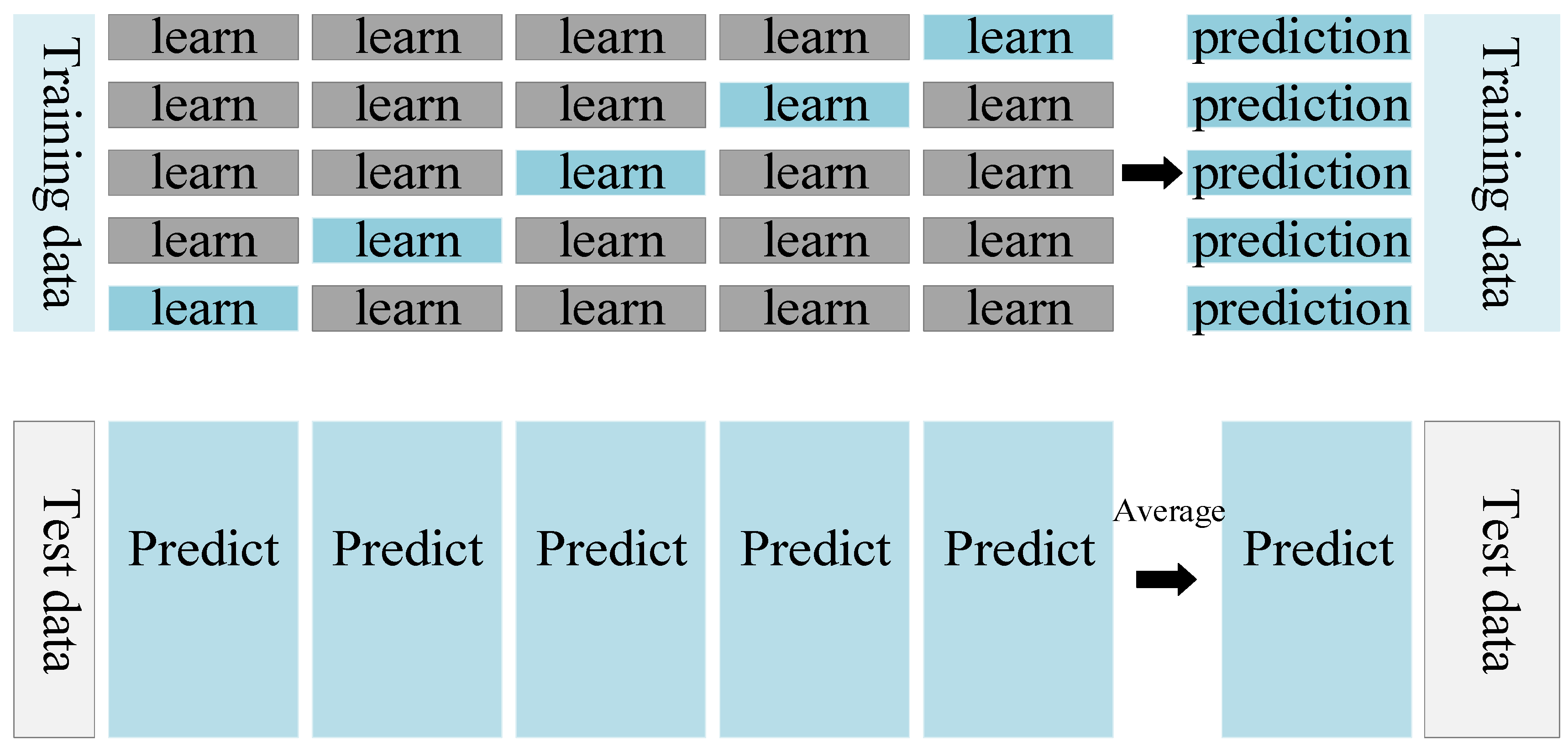
The above related studies were carried out based on single-parameter estimation. However, there is a certain coupling link between the SOC and the SOH. For example, when estimating the SOC, the variation in the maximum capacity of the battery needs to be taken into account, and at the same time, inaccurate SOC estimation will also affect SOH correction. It follows that there will also be some overlap in the estimation steps for these two parameters. SOH estimation using charge state data can not achieve online estimation. Therefore, conducting a study on the joint estimation of SOC and SOH can save certain computational steps and has high practical significance. Both for SOC estimation and SOH estimation, the data-driven method relies heavily on the choice of algorithm. However, a single data-driven algorithm is susceptible to the influence of the dataset itself, which leads to a reduced generalization ability. The integrated learning approach is particularly suitable for large datasets and nonlinear data, and is applicable to the study of the health state of lithium-ion batteries. Compared with a single model, the stacking algorithm can improve the prediction performance by integrating the advantages of multiple models. It can reduce the bias and variance of individual models and provide more stable and reliable estimation results. In addition, stacking algorithms can also improve robustness to uncertainty and noise through the diversity of models. However, the integrated learning approach tends to consume a lot of computational resources and time to build high-precision models, and the combination of Bayesian algorithms and integrated learning for training can greatly reduce the training time.
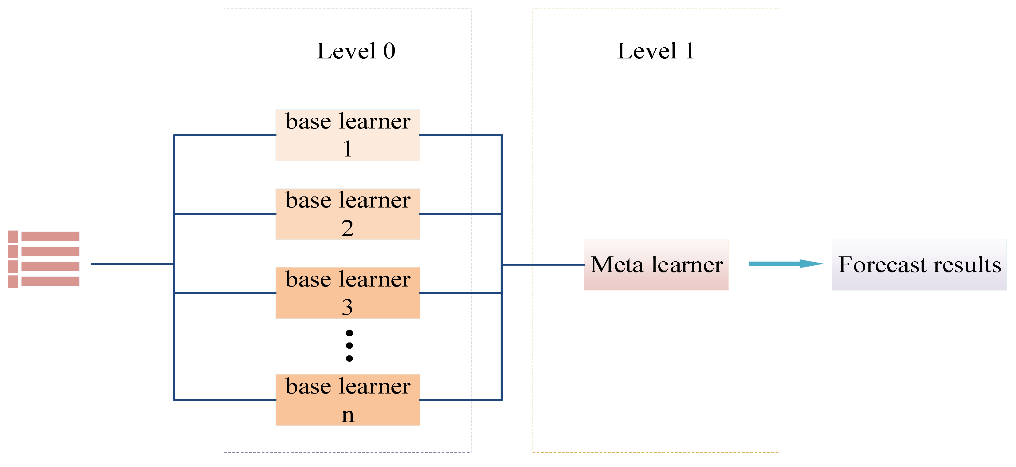
In summary, in order to predict SOC and SOH better and more accurately, and to reduce the loss of accuracy of the model, after analyzing the discharge data of NASA’s batteries, temperature and end voltage were selected as training features in this study. After that, training and testing on the dataset using LR, ENR, DTR, ETR, GBR, SVR, KNNR, DTR, and XGBoost algorithms were carried out to compare the prediction result errors of different algorithms. With LR as the meta-learner, DTR/ENR/ETR/KNNR are selected as the base learners to build the stacking integrated learning model, which is trained using the B0005 battery data and optimized using a Bayesian algorithm to optimize the parameters to predict the B0007 and B0018 batteries. Simulation analysis shows that stacking exhibits better estimation stability and accuracy than a single model. Second, this study examines the running time of the algorithm. The simulation analysis shows that the stacking algorithm does not consume too much time for the trained ground-built model, although it is an integrated learning approach. The trained model still has excellent computational speed in predicting SOH. Finally, a comparison with the estimation error results of other papers proves the effectiveness of the stacking algorithm model.

2. Algorithm Overview

2.1. Machine Learning Algorithm

The relationship between the variables in the lithium-ion battery dataset is mostly nonlinear, so the ability to adapt to nonlinearity should be considered in the algorithm selection of machine learning for individual learners. At the same time, integrated learning algorithms tend to consume a lot of computational resources, and the computational speed of machine learning algorithms should also be considered in the selection of individual learners. The main common algorithms in dealing with regression problems are KNeighbors Regressor, Decision Tree Regressor, Elastic Net, GradientBoostingRegressor, XGB Regressor, Lasso, Extra Tree Regressor, SVR, and Linear Regression. Table 1 lists the advantages and disadvantages of these mainstream algorithms as well as their scope of application. Based on the above conditions for selecting individual learners, it is considered that elastic networks and linear regression are not selected for this study due to their weak ability to handle nonlinear data. Since the meta-learner needs to deal with relatively large datasets consisting of the prediction results of individual learners, XGBRegressor was chosen as the meta-learner for this study due to its faster computational speed and its applicability to large datasets.

2.2. Stacking Algorithm

In recent years, stacking algorithms have achieved better results in various data mining competitions. As shown in Figure 1, the algorithm generally uses a two-layer structure, the primary learner and the secondary learner. First, the stacking algorithm trains the primary learner with the initial dataset, then computes a new dataset with the same dimension as the initial dataset consisting of the results of the primary learner’s operations, and then trains the secondary learner with the new dataset.
In this thesis, the 5-fold cross-validation method is used to divide the data to reduce the risk of overfitting. In order to better understand the learning process of the stacking algorithm, it is assumed that there are five primary learners (learner A, learner B, learner C, learner D, learner E) of the stacking algorithm and 5-fold cross validation is used. Figure 2 gives the specific steps of the algorithm to materialize the process: the upper half is the training set and the lower half is the test set. The training process for one learner (learner A) is shown in the figure. After 5-fold cross-validation and dividing the training set into 5 equal parts, learner A will end up with a new set of data that has the same dimensions as the training set. Similarly, the other four learners, B, C, D, and E, will go through the same operation as learner A, and produce new data, b, c, d, and e, with the same dimensions as the training set. Subsequently, the new data, a, b, c, d, and e, are averaged to obtain a new datum, “T”, with the same dimension as the training set. The test set will be operated in the same way as the training set, and new data, the “test data”, with the same dimension as the test set will be obtained. This new datum, “T”, is the training set for the secondary learner. After training the sub-learners with the new datum, “T”, the sub-learners will predict the new test set, “test data”, and the final prediction will be obtained.

2.3. Bayesian Optimization Algorithm

Before establishing the final SOC estimation model, it is necessary to adjust the important parameters in the model to achieve the optimal state as much as possible. Model parameter tuning is a very tedious and important task. When the model building enters the parameter tuning stage, it means that the work is coming to an end. The Bayesian optimization (BO) algorithm is a model hyper-parameter optimization method, which can greatly reduce the tuning time of the stacking algorithm.
Suppose a set of hyper-parameters is combined as X = x 1 , x 2 , , x n . Different combinations of hyper-parameters will give different results to the model, and the aim of Bayesian optimization is to select the hyper-parameters that give the best results to the model. The Bayesian optimization process is as follows:
The function f ( x ) needs to find an x X , such that
x * = arg min f ( x )
where x * refers to the hyperparameter.
Since it is not possible to determine the convexity of the function f ( x ) , the problem needs to be solved based on the sequence model. The algorithm is as follows:
Step 1: Determine the hyperparameter search interval ( X ) and the collection function (S) of the function f ( x ) .
Step 2: Determine the dataset (D); each pair of arrays in the dataset is denoted as (x,y). x denotes a set of hyperparameters and y denotes the output result corresponding to the hyperparameters.
Step 3: Fit the model (M) to the dataset (D) and find the specific function representation of the model.
ρ ( y | x , D ) = model ( M , D )
Step 4: Find the set of variable points (x) corresponding to make S ( x , ρ ) obtain the maximum value, i.e,
x i = arg max S ( x , ρ ( y | x , D ) )
x i is a set of hyperparameters selected by the acquisition function.
Step 5: Substitute x i into the function f ( x ) , and obtain the output value, y.
Step 6: Update the dataset (D).
D = D ( x i , y i )
Step 7: Return to step 3 and continue to select hyperparameters ( x i ); loop T times to stop.

3. Data Analysis

3.1. Li-Ion Battery Capacity Degradation Data

This study mainly uses the public battery data provided by NASA as the simulation experiment data. The battery model is a lithium iron phosphate battery. The battery numbers used in this study are B0005, B0018, and B0007. The nominal capacity is 2 Ah. The batteries were operated in three operating conditions: charging, discharging, and measuring internal resistance. The three operating conditions were all in the same room temperature (24 °C) environment. The battery was first charged with a constant current of 1.5 A until the voltage reached 4.2 V, and then with a constant voltage until the current dropped below 20 mA. In the discharge stage, the battery was discharged with a constant current of 2 A until the voltage reached 4.2 V, which is the corresponding discharge cut-off voltage. The relevant working conditions of the battery are shown in Table 1.

3.2. Raw Data Analysis

The SOC is defined as the ratio between the battery’s current remaining charge and its actual capacity. For practical purposes, it is generally calculated based on the amount of power that has been released from the battery.
S O C ( t ) = ( 1 0 t I ( t ) d t C m ) × 100 %
where I represents the current, the integral of I over [0,t] represents the amount of power discharged by the battery, and C m represents the actual capacity of the battery at the present time.
As the usage time of a battery increases, its internal irreversible aging reaction will gradually intensify, externally manifesting the phenomenon of a decreasing actual capacity, C m . Therefore, the SOH of a battery is usually defined from the perspective of capacity:
S O H = C m C 0 × 100 %
where C 0 represents the rated capacity of the battery at the factory.
Figure 3 illustrates the SOH diagram of the battery. A battery is considered to fail when the capacity decays to 70% of the rated capacity. From Figure 3, it can be seen that the capacity of battery B0018 decreases faster than that of batteries B0005 and B0007, the capacity of battery B0007 decreases slower than that of battery B0005, and the capacity of battery B0007 does not decrease to the failure threshold. The data of battery B0005 cover all the cases of the battery as much as possible, so they can be used as the training data and the other two batteries are used as the test set.

3.3. Feature Selection

Figure 4 shows a schematic of the discharge temperature of the B0005 battery. As the number of cycles increases, the temperature of the battery gradually increases, indicating that the internal impedance of the battery is gradually increasing. Therefore, the internal temperature of the battery can also be used as a characteristic of the battery. Under the actual working conditions of the battery, it is not convenient to measure the internal resistance of the battery, which limits the amount of aging. Therefore, we can determine the aging degree of the battery by analyzing the internal temperature of the battery. Figure 5 shows the discharge voltage curve of the B0005 battery. As the number of cycles increases, the slope of the battery discharge voltage curve gradually changes from flat to steep, indicating that this voltage can be used as one of the characteristic quantities for measuring battery aging. Figure 6 is a plot of the battery charge state versus time, which clearly shows that the battery charge state decreases at a progressively greater rate of SOC decline as the health of the battery decays. Therefore, the battery state of charge is an important characteristic quantity as a measure of battery aging.
From the above findings, it can be seen that the characteristic quantifiers of battery aging can be the discharge voltage, charge state, and discharge time of the battery. Therefore, the health of the battery can be judged by the analysis of these three quantities. In summary, the coupling of the SOC with the temperature and voltage is plotted, as shown in Figure 7 and Figure 8. It is difficult to determine the value of the estimated SOC by voltage or temperature alone, so SOH coupling thermograms of temperature, voltage, and SOC are plotted next, and the determined SOC, discharge time, and discharge voltage can correspond to a unique SOH.
As can be seen from Figure 9, the SOH of the cell gradually decreases. When the color changes from blue to deep red, it indicates that the aging of the battery deepens. A total of 168 discharge curves are plotted in the figure, and each curve represents a different battery SOH state, which is indicated by the color bar on the right side of the figure. Therefore, the predicted expression for SOH is as follows:
S O H = F ( S O C , U , T e m )
However, if the SOH of the battery is predicted directly by the above method, it will put a great computational pressure on the computer and the corresponding storage space is very limited. Therefore, a novel SOC–SOH coupling relationship is used in this study to simplify the computational complexity. When determining the z-axis SOC value, it will correspond to a two-dimensional coordinate (U,T), and the above information can be used to determine the discharged battery health profile. Using this feature, the battery SOH can be predicted based on a machine learning model with the estimated expression:
S O H = F ( T e m S O C = 100 % , U S O C = 100 % , T e m S O C n o w , U S O C n o w )

3.4. Model Accuracy

In this study, the root mean square error (RMSE) and determinant coefficient (R2 score), two indexes used to describe the prediction error, are used to evaluate the accuracy of the ML model. The expressions are as follows:
R 2 = 1 1 n i = 1 n ( y i y i ) 2 1 n i = 1 n ( y i y i ) 2
R M S E = 1 n i = 1 n ( y y i ) 2
The closer the value of R2 is to 1, the better the model performance; the closer the value of RMSE is to 0, the better the model performance.

3.5. General Workflow of the Model

The overall training process of the model in this study is shown in Figure 7. First of all, the two features of voltage and temperature are found by analyzing the data; then, the coupling relationship of the SOC and SOH for estimating the SOH is established. Next, the appropriate stacking model is selected by training on the B0005 dataset; finally, the selected model with stable performance is used to train and make predictions.

4. Results and Discussion

All training in this study was carried out on the same device, and the CPU of the device used was an Intel(R) Core (TM) i7-6700HQ CPU @ 2.60 GHz. In order to verify the above selection of individual learners and meta-learners, this study first uses the B0005 battery dataset to train and predict different machine learning algorithms.
The main common algorithms in dealing with regression problems are KNeighbors Regressor, Decision Tree Regressor, Elastic Net, GradientBoostingRegressor, XGB Regressor, Lasso, Extra Tree Regressor, SVR, and Linear Regression. Table 1 lists the advantages and disadvantages of these mainstream algorithms as well as their scope of application. A box plot is used to reflect the center position and scattering range of the continuous-type data distribution. The results of the overall health status estimation of B0005 are represented by a box plot as shown in Figure 7 below, with the median represented by a short red line, the two horizontal lines above and below the box representing the upper and lower boundaries of the data (the upper edge value is not necessarily the maximum value in the data, and the smallest lower edge value is not necessarily the minimum value), and the red dots representing the outliers that are beyond the upper and lower boundaries. On the far right is the raw SOH data for cell B0005. As shown in the figure, its data spread is basically uniform, and the red line is closer to the lower quartile, indicating that the original data are in a slightly left-biased state.
By observing the distribution of the other algorithm boxplots, it can be seen that the data predicted by each algorithm are in different degrees of bias. Among them, the predicted data of DTR\ETR\GBR\KNNR\SVR\XGBR have a similar distribution to the original data, DTR\ENR\ETR\LRXGBR\SVR basically shows a left-skewed state, and KNNR\LASSO shows a right skewed state. The DTR\LASSO\LR\SVR algorithm shows outlier points, and all of them are below the lower boundary, indicating that the errors of the algorithms are mostly the predicted values being smaller than the actual values. Regarding the prediction results made by the LR and LASSO algorithms, the median red line is shifted too much and the box is too narrow, showing that the predicted values of these two algorithms are concentrated in a certain interval and do not have the ability to predict directly. Figure 8 shows the R2 score of the algorithms as well as the RMSE values, and it can be seen that the R2 score of the best-performing model also stays below 0.8, indicating that the predictive ability of a single model needs to be further improved.
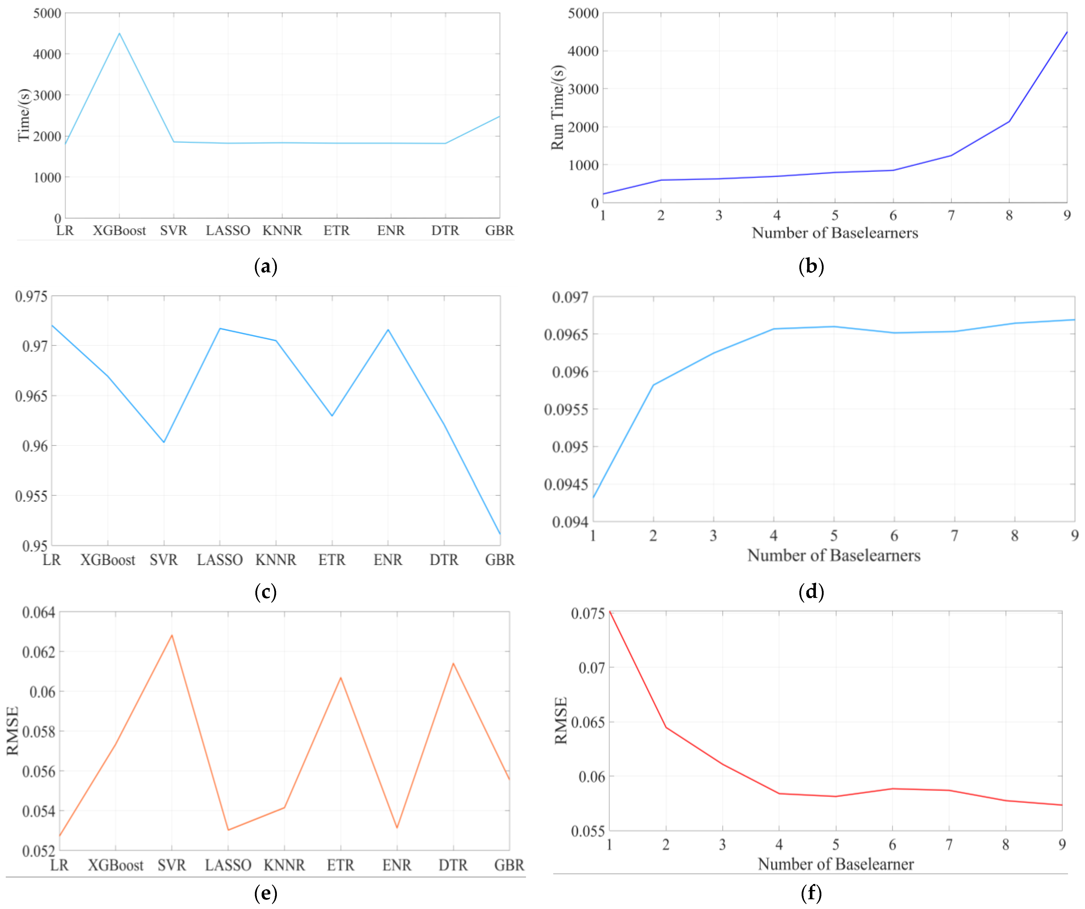
Considering the characteristics of stacking algorithms, appropriate individual learners and meta-learners will be selected by experiments. Nine machine learning algorithms are first used as base learners/meta-learners, the stacking algorithm is trained and predicted on the B0005 dataset, and the training set is divided into 9:1 with the test set. The results are shown in Figure 9 below.
Figure 9a shows the training time of different algorithms as meta-learner models. It can be seen that the overall model training is time-consuming when XGBoost is used as the meta-learner; other algorithms, except GBR, have similar model training times; and when LR is used as the meta-learner, the shortest model training runtime is 1795.4763 s. Figure 9b shows the R2 scores of the models of different algorithms as meta-learners. Figure 9c shows the training errors of the models of different algorithms as meta-learners. Combining Figure 9b,c, it is found that LR as a meta-learner has the highest R2 score of 0.972 and the lowest RMSE of 0.05272498 compared to the other algorithms. So, it was finally decided to use LR as a meta-learner for modeling.
After determining the meta-learner, the number of base learners and the algorithm chosen still need to be further determined. A method using the addition of different base learners one by one was carried out next and used to determine the final base learner. A total of nine different machine learning algorithms were selected for this study. Firstly, only DTR was used as the base learner to train and test on the dataset. Secondly, the ENR algorithm was added to build the model with two base learners for training, and in this way, these nine algorithms were added as base learners to build the model in turn. The results of the experiment are shown in Figure 10 below. Figure 10a represents the training time of the model with different numbers of base learners, and it can be observed that the rate of increase of the training time of the whole model gradually becomes larger after using the SVR algorithm to constitute seven base learner algorithms. Figure 10b shows the R2 scores of the models with different numbers of base learners, and it can be observed that before using four base learners, the R2 score gradually increases with the growth of the learners and then basically remains stable, except for the decrease after the addition of the two algorithms of LR/SVR. Figure 10c represents the training errors of models with different numbers of base learners. As can be seen from the figure, the error decreases with the increase in the number of base learners, which is most obvious before the number of base learners is increased to four. To summarize, the construction of the stacking algorithm should be considered from the three aspects of reducing the training time, improving the accuracy, and decreasing the error. After balancing, the final choice is to construct the stacking model with four base learners with the DTR/ENR/ETR/KNNR algorithm.
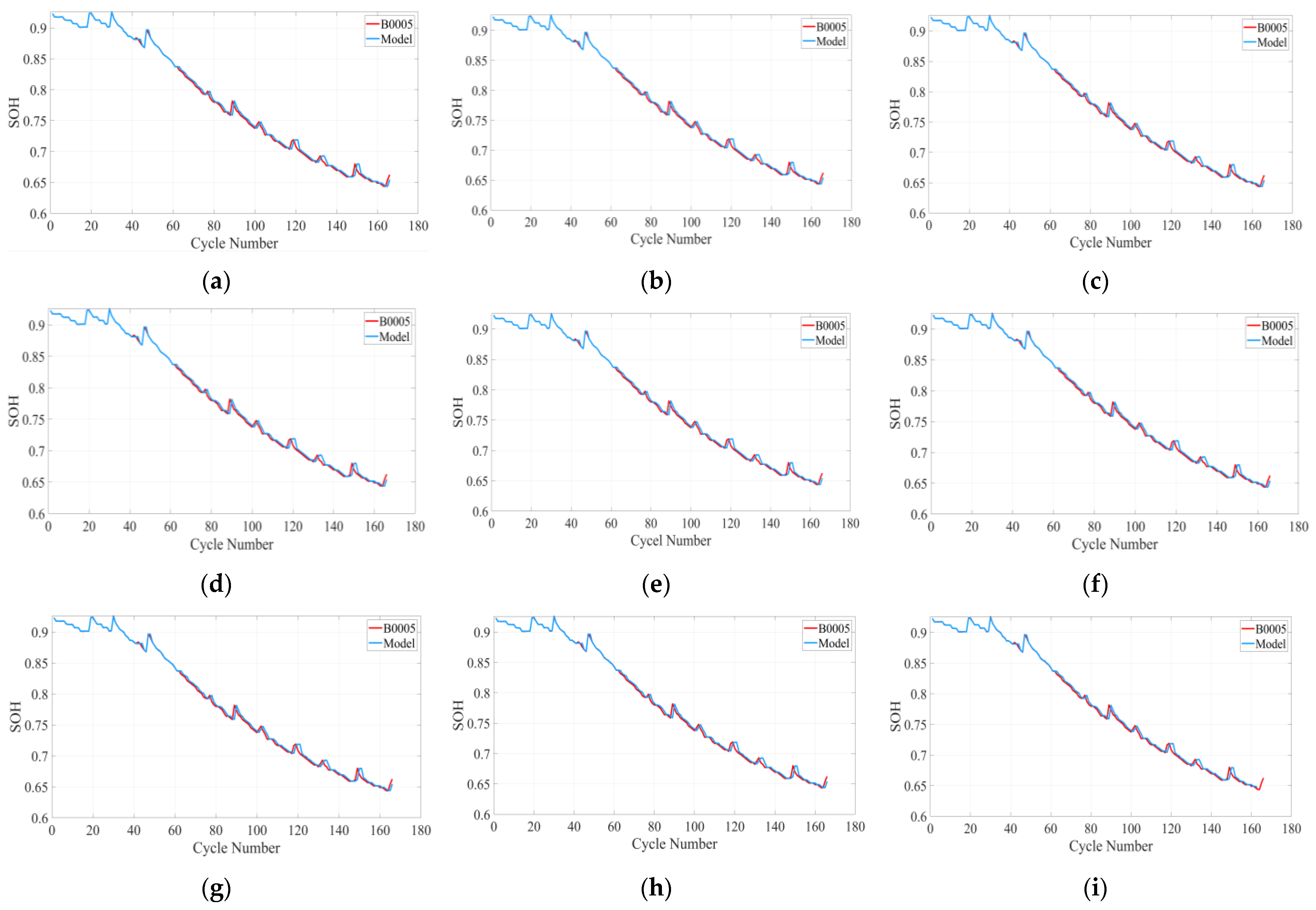
After constructing the model, the B0005 battery is used as the training data to predict the SOC. The battery state of charge is evaluated sequentially and substituted into the established joint SOC–SOH estimation model. Nine SOC interval segments are selected to reflect the estimation effect of the model. The SOH estimation effect is shown in Figure 11. From the figure, it can be seen that the constructed stacking model has a stable overall estimation effect. The performance of the model was evaluated using the root mean square error (RMSE) and the results are shown in Table 2. The R2 score is maintained around 0.997 and the RMSE results are basically unchanged, indicating that the model performs stably and accurately in predicting the SOH.
To verify the generalization ability of the model, the discharge current and terminal voltage are still used as features to make predictions about the health status of lithium-ion batteries of models B0007 and B0018. The results are shown in Figure 11a,b, where the raw data are in blue. The prediction of B0007 takes 0.48 ms, and the prediction of B0018 takes 0.32 ms. As can be seen from Table 2, Table 3 and Table 4 combined with Figure 11a,b, the stacking algorithm in this study not only does not have the phenomenon of overfitting, but also shows a strong generalization ability.

5. Conclusions

Most data-driven methods can provide an accurate estimate of the health status of lithium batteries, effectively reducing the risks and losses caused by failures during use. However, a single data-driven algorithm is susceptible to the influence of the dataset itself, resulting in lower accuracy. In addition, since the relationships between variables in the lithium-ion battery dataset are mostly nonlinear, it is very difficult to establish an accurate SOH fitting relationship on the discharge dataset using a model. Meanwhile, most of the related studies on battery health estimation are offline estimation, and the inability to estimate online is also a problem to be solved. In view of such problems, this study proposes a joint machine learning SOC–SOH estimation method based on a stacking algorithm, which realizes online detection and the estimation of battery management systems.
Firstly, this study utilized the publicly available data of batteries provided by NASA as the simulation experimental data, and explored the SOH changes of different characteristic responses by plotting the end-voltage curve, the discharge current curve, the SOC-time curve, etc., and finally chose the end-voltage and the temperature as the input characteristics.
Secondly, starting from the basic algorithm of a single model, this study analyzed the prediction ability of each of the different tree modeling algorithms of Decision Tree, GBR, SVR, KNeighbors Regressor, Extra Tree Regressor, and XGBoost, and chose the stacking integrated learning method, with LR as the meta-learner and the other four algorithms as the sub-learners.
Finally, this study used the B0005 battery as the training set, used the Bayesian algorithm for parameter optimization, and used the trained model for the SOH prediction of the B0007 and B0018 batteries. After a comparative analysis, the developed models were found to have a strong generalization ability, and the running time for the prediction of the full dataset was less than 0.2 ms, which indicates the great potential of actual linear estimation.

Author Contributions

Investigation, Y.D. and K.C.; methodology, Y.D. and G.Z.; software, Y.D.; visualization, R.L.; writing—original draft preparation, Y.D. and K.C.; writing—review and editing, G.Z. and R.L. All authors have read and agreed to the published version of the manuscript.

Funding

This work was supported by the “Heilongjiang Provincial Natural Science Foundation of China (No. ZD2023B001)”.

Data Availability Statement

Publicly available datasets were analyzed in this study. This data can be found here: https://ti.arc.nasa.gov/tech/dash/groups/pcoe/prognostic-data-repository/ (access on 9 January 2024).

Conflicts of Interest

The authors declare no conflicts of interest.

References

  1. Alola, A.A.; Olanipekun, I.O.; Shah, M.I. Examining the drivers of alternative energy in leading energy sustainable economies: The trilemma of energy efficiency, energy intensity and renewables expenses. Renew. Energ. 2023, 202, 1190–1197. [Google Scholar] [CrossRef]
  2. Li, R.; Li, W.; Zhang, H.; Zhou, Y.; Tian, W. On-line estimation method of lithium-ion battery health status based on PSO-SVM. Front. Energy Res. 2021, 9, 693249. [Google Scholar] [CrossRef]
  3. Lin, P.; Jin, P.; Zhang, H. Identification and Fast Measurement Method of Open-circuit Voltage. J. Electrochem. Soc. 2023, 170, 030525. [Google Scholar] [CrossRef]
  4. Pavković, D.; Kasać, J.; Krznar, M.; Cipek, M. Adaptive Constant-Current/Constant-Voltage Charging of a Battery Cell Based on Cell Open-Circuit Voltage Estimation. WEVJ 2023, 14, 155. [Google Scholar] [CrossRef]
  5. Li, W.; Ruan, S.; Bahitbek, A.; Gao, Z.; Turak, N.; Li, H. Exploring the Hysteresis Effect in SOC Estimation of Li-ion Batteries. J. Phys. Conf. Ser. IOP Publ. 2023, 2456, 012023. [Google Scholar] [CrossRef]
  6. Wang, Q.; Qi, W. New SOC estimation method under multi-temperature conditions based on parametric-estimation OCV. J. Power Electron. 2020, 20, 614–623. [Google Scholar] [CrossRef]
  7. Lin, M.; Yan, C.; Wang, W.; Dong, G.; Meng, J.; Wu, J. A data-driven approach for estimating state-of-health of lithium-ion batteries considering internal resistance. Energy 2023, 277, 127675. [Google Scholar] [CrossRef]
  8. Korkmaz, M. SoC estimation of lithium-ion batteries based on machine learning techniques: A filtered approach. J. Energy Storage 2023, 72, 108268. [Google Scholar] [CrossRef]
  9. Zhao, S.; Zhang, C.; Wang, Y. Lithium-ion battery capacity and remaining useful life prediction using board learning system and long short-term memory neural network. J. Energy Storage 2022, 52, 104901. [Google Scholar] [CrossRef]
  10. Zhou, W.; Zheng, Y.; Pan, Z.; Lu, Q. Review on the battery model and SOC estimation method. Processes 2021, 9, 1685. [Google Scholar] [CrossRef]
  11. Togasaki, N.; Yokoshima, T.; Oguma, Y.; Osaka, T. Prediction of overcharge-induced serious capacity fading in nickel cobalt aluminum oxide lithium-ion batteries using electrochemical impedance spectroscopy. J. Power Sources 2020, 461, 228168. [Google Scholar] [CrossRef]
  12. Zhang, X.; Gao, Y.; Guo, B.; Zhu, C.; Zhou, X.; Wang, L.; Cao, J.H. A novel quantitative electrochemical aging model considering side reactions for lithium-ion batteries. Electrochim. Acta 2020, 343, 136070. [Google Scholar] [CrossRef]
  13. Hou, M.; Hu, Y.; Zhang, J.; Cao, H.; Wang, Z. Development of electrochemicalthermal modelling for large-format Li-ion battery. Electrochim. Acta 2020, 347, 136280. [Google Scholar] [CrossRef]
  14. Amir, S.; Gulzar, M.; Tarar, M.O.; Naqvi, I.H.; Zaffar, N.A.; Pecht, M.G. Dynamic equivalent circuit model to estimate state-of-health of lithium-ion batteries. IEEE Access 2022, 10, 18279–18288. [Google Scholar] [CrossRef]
  15. Yang, J.; Cai, Y.; Mi, C.C. State-of-health estimation for lithium-ion batteries based on decoupled dynamic characteristic of constant-voltage charging current. IEEE Trans. Transp. Electrif. 2021, 8, 2070–2079. [Google Scholar] [CrossRef]
  16. Chen, M.; Wu, J.; Jiao, C.; Chen, J.; Zhang, Z. Multi-Factor online estimation method for health status of lithium-ion battery. Hsi-An Chiao Tung Ta Hsueh/J. Xi’an Jiaotong Univ. 2020, 54, 169–175. [Google Scholar]
  17. Zhang, Q.; Wang, D.; Yang, B.; Cui, X.; Li, X. Electrochemical model of lithium-ion battery for wide frequency range applications. Electrochim. Acta 2020, 343, 136094. [Google Scholar] [CrossRef]
  18. Zhou, L.; Zhang, Z.; Liu, P.; Zhao, Y.; Cui, D.; Wang, Z. Data-driven battery state-of-health estimation and prediction using IC based features and coupled model. J. Energy Storage 2023, 72, 108413. [Google Scholar] [CrossRef]
  19. Li, X.; Ju, L.; Geng, G.; Jiang, Q. Data-driven state-of-health estimation for lithium-ion battery based on aging features. Energy 2023, 274, 127378. [Google Scholar] [CrossRef]
  20. Waseem, M.; Huang, J.; Wong, C.N.; Lee, C.K.M. Data-driven GWO-BRNN-based SOH estimation of lithium-ion batteries in EVs for their prognostics and health management. Mathematics 2023, 11, 4263. [Google Scholar] [CrossRef]
Figure 1. Algorithm structure.
Wevj 15 00075 g001
Figure 2. Algorithm process.
Wevj 15 00075 g002
Figure 3. Battery capacity degradation.
Wevj 15 00075 g003
Figure 4. (a) Discharge temperature diagram of a battery; (b) the discharge voltage curve of a battery; (c) SOC–time relationship diagram of a battery.
Wevj 15 00075 g004
Figure 5. (a) SOC–temperature relationship diagram of a battery; (b) SOC–Voltage relationship diagram of a battery.
Wevj 15 00075 g005
Figure 6. T/U-SOC and SOH coupling diagram.
Wevj 15 00075 g006
Figure 7. Overall training process.
Wevj 15 00075 g007
Figure 8. (a) Model predicted SOH boxplot; (b) SOH prediction model R2-RMSE.
Wevj 15 00075 g008
Figure 9. (a) The runtime of algorithms using different meta-learners; (b) the R2 score of algorithms using different meta-learners; (c) the RMSE of algorithms using different meta-learners; (d) the runtime of algorithms using different numbers of base learners; (e) the R2 score of algorithms using different numbers of base learners; (f) the RMSE of algorithms using different meta-learners.
Wevj 15 00075 g009
Figure 10. Estimation of SOH in different states of charge: (a) SOC change (100–10%), (b) SOC change (100–20%), (c) SOC change (100–30%), (d) SOC change (100–40%), (e) SOC change (100–50%), (f) SOC change (100–60%), (g) SOC change (100–70%), (h) SOC change (100–80%), (i) SOC change (100–90%).
Wevj 15 00075 g010
Figure 11. (a) SOH prediction of battery B0007; (b) SOH prediction of battery B0018.
Wevj 15 00075 g011
Table 1. The advantages, disadvantages, and applicable conditions of common machine learning algorithms.
Model NameAdvantageDisadvantageApplicability
KNeighbors RegressorPerforms well on small datasets
Applicable to regression problems
Poor performance on high-dimensional data
High computational cost for big datasets
Small dataset
Decision Tree RegressorGood performance for nonlinear dataEasy to overfit
Poor performance on high-dimensional data
nonlinear dataset
Elastic NetCan handle high-dimensional data
Not sensitive to noise
Poor performance on nonlinear data
High computational cost
high-dimensional dataset
Gradient Boosting RegressorGood performance for nonlinear data
Not sensitive to noise
Sensitive to hyperparametersnonlinear dataset
XGB RegressorFast calculation speed
High accuracy
Performs well on big datasets
Sensitive to hyperparameterslarge dataset
LassoCan handle high-dimensional data
Not sensitive to noise
Poor performance on nonlinear data
High computational cost
high-dimensional dataset
Extra Tree RegressorFast calculation speed
Not sensitive to noise
Could handle nonlinear data
Easy to overfit
Method is sensitive to hyperparameters
nonlinear dataset
SVRCan handle nonlinear data
Not sensitive to noise
Sensitive to hyperparameters
Poor performance on big datasets
nonlinear dataset
Linear RegressionLow computational cost
Performs well on linear data
Poor performance on nonlinear data
Sensitive to noise
linear dataset
KNeighbors RegressorPerforms well on small datasets
Applicable to regression problems
Poor performance on high-dimensional data
High computational cost for big datasets
Small dataset
Decision Tree RegressorGood performance for nonlinear dataEasy to overfit
Poor performance on high-dimensional data
nonlinear dataset
Elastic NetCan handle high-dimensional data
Not sensitive to noise
Poor performance on nonlinear data
High computational cost
high-dimensional dataset
Table 2. Battery charging and discharging working status.
Battery
Number
Charge
Cutoff
Voltage (V)
Discharge Cutoff
Voltage (V)
Charging
Current (A)
Discharge
Current (A)
Rated
Capacity (Ah)
B00054.22.71.522
B00074.22.51.522
B00184.22.51.522
Table 3. Model performance results.
SOC100–10%100–20%100–30%100–40%100–50%100–60%100–70%100–80%100–90%
R20.99780.99770.99760.99680.99770.99750.99980.99780.9964
RMSE0.00440.00440.00470.00560.00540.00450.00540.00340.0054
Table 4. Optimization results.
Battery NumberR2RMSE (%)
B00050.99760.044
B00070.99740.0041
B00180.99630.0047
Disclaimer/Publisher’s Note: The statements, opinions and data contained in all publications are solely those of the individual author(s) and contributor(s) and not of MDPI and/or the editor(s). MDPI and/or the editor(s) disclaim responsibility for any injury to people or property resulting from any ideas, methods, instructions or products referred to in the content.

