Article

Sizing of Autonomy Source Battery–Supercapacitor Vehicle with Power Required Analyses

by
Juliana Lopes
*,
José Antenor Pomilio
* and
Paulo Augusto Valente Ferreira
Department of Energy and Systems, School of Electrical and Computer Engineering, Universidade Estadual de Campinas (UNICAMP), Campinas 13083-852, Brazil
*
Authors to whom correspondence should be addressed.
World Electr. Veh. J. 2024, 15(3), 76; https://doi.org/10.3390/wevj15030076
Submission received: 13 December 2023 / Revised: 8 February 2024 / Accepted: 14 February 2024 / Published: 20 February 2024
(This article belongs to the Special Issue Propulsion Systems of EVs 2.0)

Abstract

:
The combined use of batteries and supercapacitors is an alternative to reconcile the higher energy density of batteries with the high power density of supercapacitors. The optimal sizing of this assembly, especially with the minimization of mass, is one of the challenges of designing the power system of an electric vehicle. The condition of the unpredictability of the power demand determined by the vehicle driver must also be added, which must be met by the power system without exceeding safe operating limits for the devices. This article presents a methodology for minimizing the mass of the electrical energy storage system (ESS) that considers the various aspects mentioned and a variety of battery technologies and supercapacitor values. The resulting minimum mass dimensioning is verified by simulation for different driving cycles under conditions of maximum power demand. The system also includes a tertiary source, such as a fuel cell, responsible for the vehicle’s extended autonomy. In addition to sizing the ESS, the article also proposes a management strategy for the various sources to guarantee the vehicle’s expected performance while respecting each device’s operational limits.

1. Introduction

Environmental issues justify developing transportation systems using sustainable, efficient, and clean energy resources [1]. An electric vehicle (EV) can have a single type of power source, for example, batteries (BTs), or more than one type, such as BTs and supercapacitors (SCs). In this case, the EV can be identified as a hybrid electric vehicle (HEV). The strategies for integrating and managing the different power sources must address increasing the energy efficiency and the specific driving requirements of the HEVs [2,3,4,5,6,7,8].
A power source’s energy and power limits rarely meet the requirements for a particular application [9,10]. A specific source type can be chosen over another by employing the Ragone plot that provides information about the available energy and power in the sources [11]. The advantage of using Ragone plots lies in determining a safe region of operation for the sources [12].
The sizing of the sources must be compatible with the HEV power and energy requirements [10]; otherwise, there is a risk of over/under-sizing the sources. Hence, an optimal procedure that minimizes these power sources’ size and costs is necessary [13,14]. Usually, in the literature, these methodologies aim for a cost-effective system of hybrid power sources [2,10,15]. Moreover, some studies have addressed problems of sizing and energy management in codependence [16,17].
Researchers Huilong and Cao [16] investigated the sizing and real-time energy management of an electric race car model. The authors proposed a multi-objective Bi-level optimal sizing that finds optimal energy management parameters beyond the energy storage system (ESS) sizing. In [17], the goals of working with source sizing in codependency with energy management were achieved, and the installation costs were minimal. Here, the authors explain the main two approaches—probabilistic and deterministic—used to characterize the driving cycle’s variables. The first one is generally applied to vehicles with a general purpose [18,19], and in the other approach, those variables are regarded as deterministic [20,21]. This second approach is generally used in vehicles with a predefined driving pattern, such as city buses.
However, these studies do not analyze the required power profile’s influence on the source sizing. Such influence is pointed out in our analysis. In the present study, we use a deterministic approach for the driving cycles and allow vehicles to be driven in a random cycle as long as the required power limits of the envelope power profile are respected.
Lopes et al. [2] and Schupbach et al. [12] presented optimal sizing procedures to minimize the mass of the ESS and the mass of the fuel cell (FC), the autonomy source. However, these authors have considered only one peak of power to apply their methodologies as a requirement. Three powertrain topologies (FC-BT, FC-SC, and FC-BT-SC) were analyzed in [12,15]. The optimal sizing in [15] included vehicle performance, fuel economy, and powertrain costs. The authors considered only the Federal Urban Driving Schedule (FUDS) driving cycle to apply their methodology.
According to [2,12,15], the problem of source sizing was addressed by optimization techniques. Among them, some differences can be noted in how the optimization was used, for example, in the formulation of the constraints or on the variables of the objective function. Despite the extensive work devoted to studying techniques of optimization and control strategies for electric vehicles, little attention has been given to the time interval of power demand for which the ESS is sized a priori.
To fill this gap, this study devotes attention to time intervals of power demand used in a reported ESS sizing methodology based on non-linear optimization [2]. Attempting to perform an ESS sizing consistent with the unpredictability of the power required, we devised a power-demand profile representing random drivability conditions. Therefore, this power-demand profile was obtained from an envelope-type power profile, which was obtained by overlapping the power required profiles of five driving cycles. These driving cycles depict urban and highway driving conditions, i.e., frequent stop-and-go and high cruising speeds. We aimed to investigate configurations with lower ESS mass to meet periods with high power peaks from the envelope power profile. Precisely, we aimed to find the optimal ESS sizing to meet the time interval of the high power demand of the envelope with no participation of the autonomy source.
Hence, it is expected that by utilizing efficient and relatively simple energy management, the vehicle should be capable of being driven in any driving condition with no compromise in its performance.
The paper was developed considering three types of batteries—lithium-ion (Li-ion), nickel metal hydride (NiMH), and lithium–sulfur (Li-S)—and two values of supercapacitors (58 F and 165 F). Hence, we have six ESS configurations: Li-ion/58 F (ESS1), Li-ion/165 F (ESS2), NiMH/58 F (ESS3), NiMH/165 F (ESS4), Li-S/58 F (ESS5), and Li-S/165 F (ESS6). All of them were sized to meet three periods of the envelope power profile. Different types of BTs and SCs were used to show the viability of the proposed ESS methodology, based on non-linear optimization, with varying power sources. The ESS with lower mass has 93.7 kg with 35 strings of Li-ion BTs and one string of 58 F SCs.
This ESS sizing methodology can be applied to other sources as long as they fit into the models used in this work and to any time-varying power demand. Because this methodology applies to periods of time-varying power demand, the source sizing is more robust despite being minimal.

2. System Modeling

This section will initially present the system modeling. This includes the vehicle’s dynamic and the BT and SC modeling.

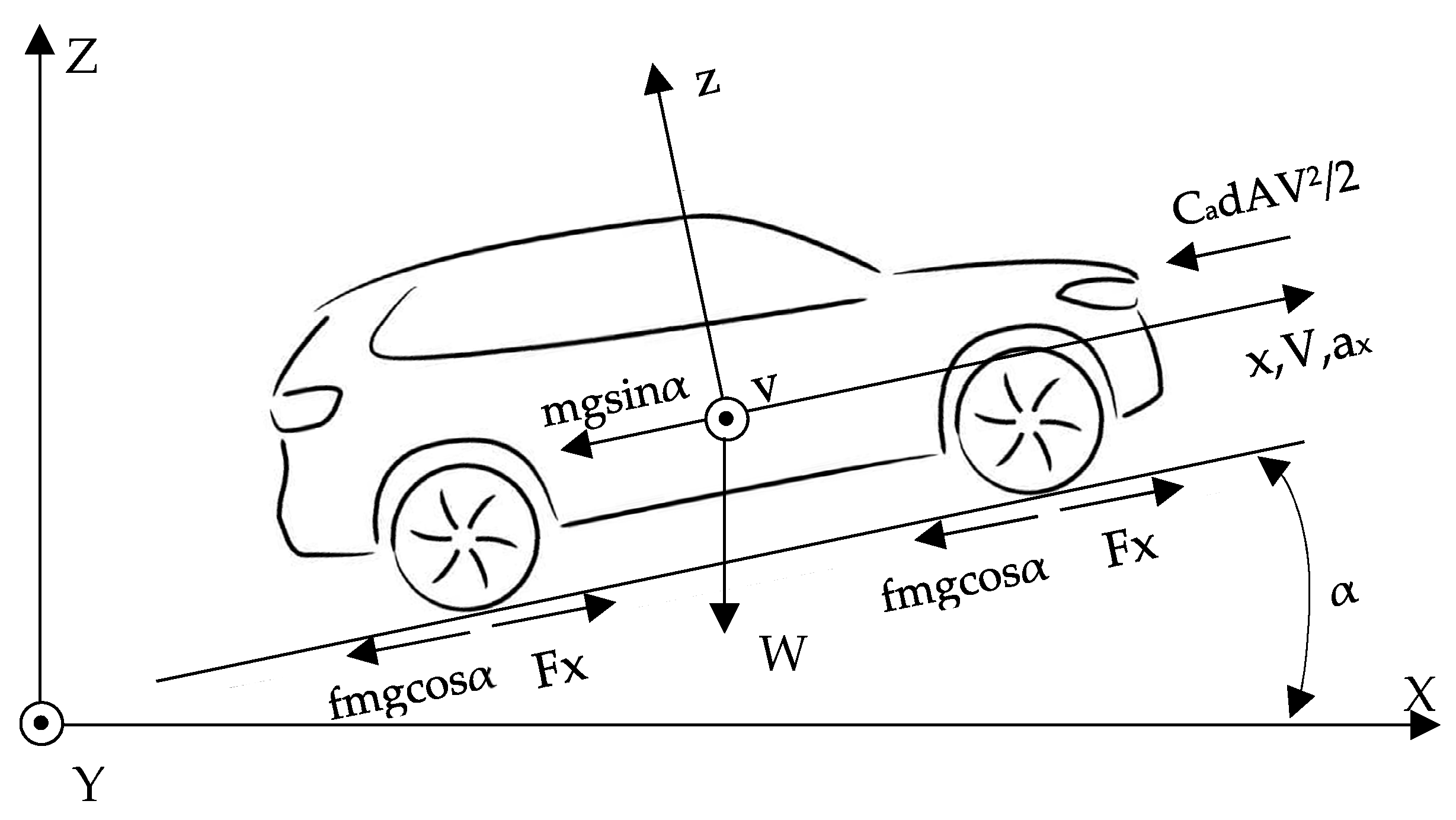
2.1. Vehicular Dynamic Modeling

The longitudinal vehicle’s dynamics considers all vehicle components as moving simultaneously [22]. In this case, the vehicle can be represented by a rigid body with a center of mass. Longitudinal vehicle dynamics deals with acceleration and braking for a vehicle driven in a straight line, in the x-direction of the Cartesian plane, as shown in Figure 1. The resistance forces acting on the longitudinal movement of the vehicle are the air resistance force, Fair:
F a i r = C a   d   A   V 2 / 2 ,
where Ca is the drag coefficient, d is the air density, A is the vehicle’s frontal area, and V is the vehicle speed. The rolling resistance force, Froll, is calculated as follows:
F r o l l = f   M   g   cos α ,
where f is the rolling resistance coefficient, M is the vehicle’s gross mass, g is the gravity acceleration, and α is the road slope angle. Lastly, the road slope resistance force, Fslope, is calculated as follows:
F s l o p e = M   g   sin α .
Therefore, the traction force transmitted to the road by the wheels is calculated as follows:
F x = M + M r a x + F a i r + F r o l l + F s l o p e ,
where Mr is the equivalent mass of the vehicle’s rotating components (driveshaft, semi-axles, and wheels) and ax is the vehicle’s acceleration. We assume that Mr is 10% of the curb weight (1548 kg).
The first term of (4) is the force required to accelerate the vehicle, and the others are the resistance forces mentioned above. The values of the main parameters, based on a sport utility vehicle (SUV) model, are in Table 1.
Multiplying (4) by “V” on both sides and assuming the road’s slope resistance is zero results in the vehicle’s required power, Preq.
P r e q = F x V = M + M r a x + F a i r + F r o l l V
Some powertrain efficiencies were considered to compute the required power: 90% for the final drive and the electric motor and 95% for the inverter and the converter. Consequently, the resulting efficiency was 73%. In summary, in acceleration, (5) is divided by 0.73, and in breaking this equation, it is multiplied by 0.73.
The autonomy source is responsible for the vehicle’s extended autonomy. Because of the existence of a hybrid ESS, the autonomy source will operate at constant power of 33 kW. This value of power is equal to the average power of the envelope power profile—analyzed in detail in Section 3.2.

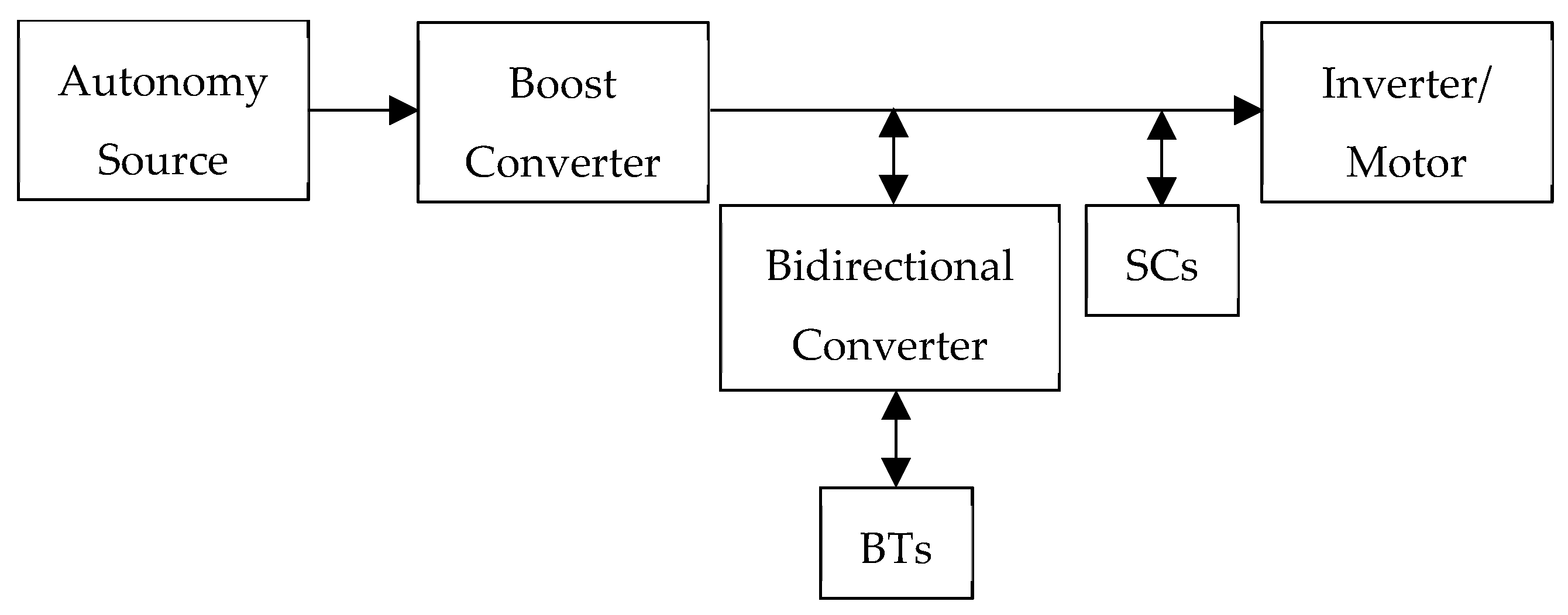
2.2. EV’s Powertrain Topology
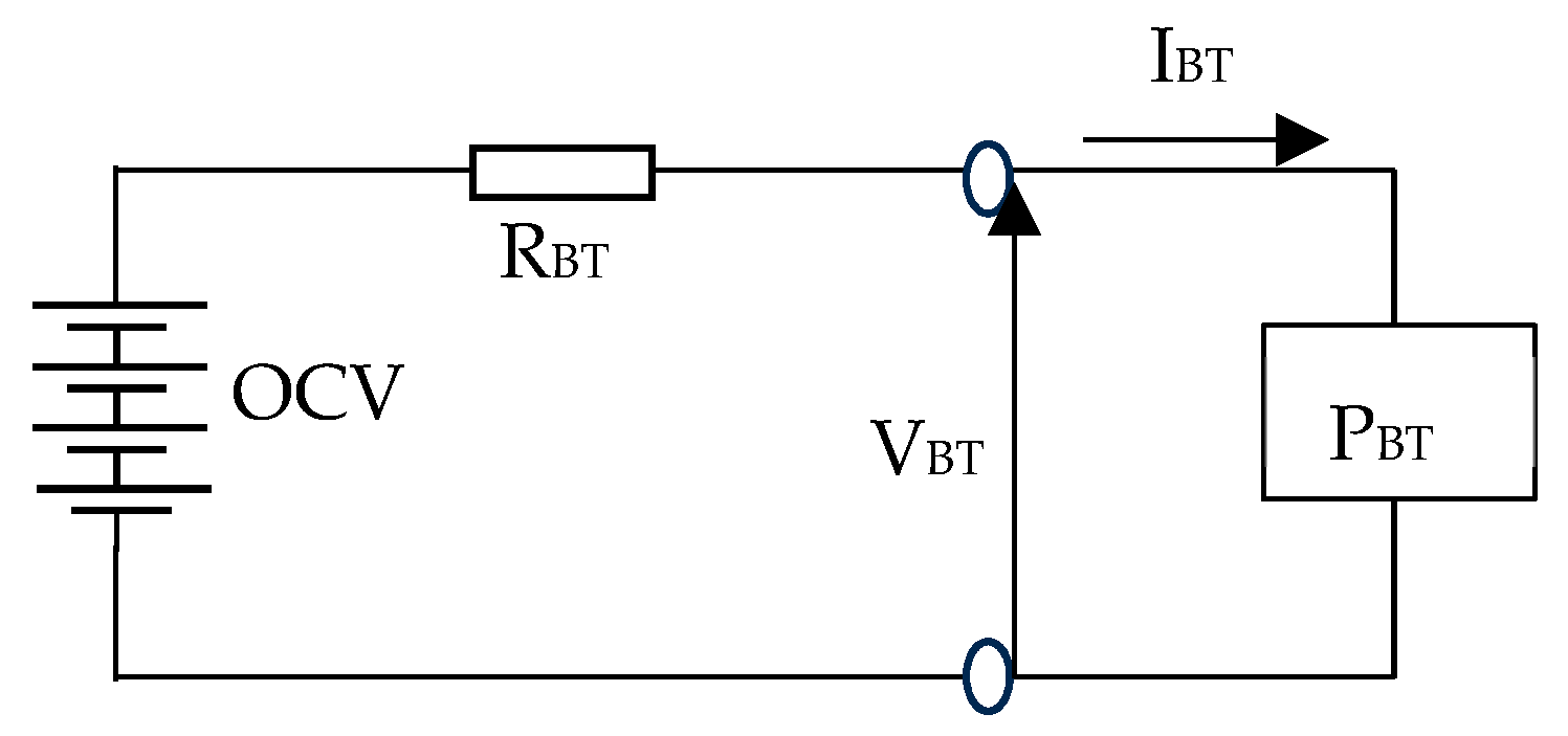
Figure 2 shows the EV’s powertrain topology used in this study. This topology is pointed out as the best choice among the analyzed ones in [15]. A bidirectional converter is used to connect the BTs to the DC bus. Because SCs are used to provide transient power, the losses associated with the operation of the bidirectional converter occur less frequently. The terminal voltage of the SCs is controlled to remain between 250 and 400 V, and the number of SCs in series is fixed. The inverter must operate at a variable voltage on the DC side.

2.3. Battery Model

As mentioned, different types of BTs and SCs were considered to show the viability of the proposed ESS sizing methodology. Among the batteries, the Li-ion type is widely used as a power source for traction in electric vehicles. This is evident in the literature and the EVs in the market [23,24,25,26,27]. Li-ion battery advantages include high energy density, low self-discharge, and high discharging rate capabilities [28,29]. However, some drawbacks, such as recycling, charging capacity, and thermal control, must be overcome [30,31,32,33].
NiMH BTs have been widely used in hybrid EVs with combustion engines [33]. Features such as long life, safety, and tolerance to overcharge/discharge make NiMH BTs suitable for use in EVs [34,35,36]. However, these batteries have disadvantages, such as high purchase cost, high self-discharge, and a relatively low energy density compared to Li-ion BTs [37].
Lastly, the third battery type that we used in this work was the Li-S BTs [38]. These batteries can be lighter and cheaper and can store much more energy than current Li-ion BTs, making them attractive as the power source of EVs. However, its short lifetime is the biggest obstacle [39]. To overcome these limitations, high-energy and safe Li-S cells have been improved to power EVs [40].
The considered equivalent electric model is the same for the three types of BTs (Figure 3). RBT is the BT’s internal resistance, OCV is the BT’s open circuit voltage, IBT is the BT’s current, VBT is the terminal voltage of BT, and PBT is the power required or supplied to the batteries.
From the BT terminal voltage (VBT), Equation (6), and the power (PBT), Equation (7), we obtain the BT current (IBT), Equation (8).
V B T = O C V R B T I B T ,
P B T = V B T I B T ,
I B T = O C V + O C V 2 4 R B T P B T / 2 R B T ,
The total charge removed from the BT, CR, in the nth simulation step is as follows:
C R n + 1 = C R n + δ t × I B T / 3600   A h ,
where δt is the time interval in seconds between sequential computations.
Therefore, the battery’s state of charge (SoCBT) is given by Equation (10):
S o C B T = 1 C R / I B T k × t ,
where k is the Peukert coefficient that estimates the effect of the current on the BT’s original capacity. If the current demand varies slowly, the battery capacity increases; otherwise, the capacity drops drastically.
The BT’s control, both for the sizing methodology and energy management, considers the relationship between the SoCBT and the OCV, often described by polynomial equations. Equations (11) and (12) describe the OCV for NiMH and Li-ion BTs, respectively [9,41].
O C V = n 0.001083   S o C B T 5 + 0.01713   S o C B T 4 0.1002   S o C B T 3 + 0.2673   S o C B T 2 0.321   S o C B T + 1.363 ,
O C V = n 108.97   S o C B T 6 + 355.88   S o C B T 5 453.64   S o C B T 4 + 284.33   S o C B T 3 90.038   S o C B T 2 + 13.433   S o C B T + 3 ,
where n is the number of cells in series. SoCBT is 1 for a fully charged battery and 0 for a discharged battery.
On the other hand, the chemical parameters of the Li-S BT, as the OCV, and the internal resistance, RBT, vary between high and low plateau patterns. Hence, there is a polynomial function for each plateau [42]. Equations (13) and (14) are the polynomial functions for the high and low OCV plateaus.
O C V h i g h = n 19.53   S o C B T 5 47.78   S o C B T 4 + 43.08   S o C B T 3 15.5   S o C B T 2 + S o C B T + 2.1 ,
O C V l o w = n 50.49   S o C B T 8 170.36   S o C B T 7 + 226.3   S o C B T 6 147.74   S o C B T 5 + 46.17   S o C B T 4 3.8   S o C B T 3 1.34   S o C B T 2 + 0.32   S o C B T + 2.11 .
A sinusoidal partial gamma function, γm,c, connects both functions smoothly, with no loss of generality.
γ m , c S o C B T = 0 , 1 / 2 + 1 / 2 sin 2 m S o C B T c , 1 , if   a if   b if   c
where a, b, and c parameters represent the different ranges of the gamma function:
a : 2 m S o C B T c < 1 / 2 π , b : 1 / 2 π 2 m S o C B T c < 1 / 2 π , c : 2 m S o C B T c > 1 / 2 π .
In [42], the OCV and RBT polynomial functions are given for different temperatures: 20, 30, and 50 °C. We consider the polynomials obtained for 50 °C. In this case, according to [42], the transition point c between Equations (13) and (14) is 0.92. The scale factor m Equation (16) determines the transition range between high and low OCV plateaus’ polynomials. The scale factor value used is 20, obtained from the condition b of Equation (16). For this value of m, the transition polynomial function will operate for SoCBT between 0.88 and 0.96. In detail, for SoCBT greater than 0.96, the polynomial function of the high plateau works, and for SoCBT less than 0.88, it is the polynomial function of the low plateau that works. Remember that the initial SoCBT is equal to 1.
Therefore, the combined function for both polynomials is as follows:
f O C V S o C B T = 1 γ m , c S o C B T f O C V l o w S o C B T + γ m , c S o C B T f O C V h i g h S o C B T .
Regarding the internal resistance of the batteries, NiMH BT’s value is constant and equal to 0.002 Ω, as reported in [43]. However, the internal resistances for the Li-ion and Li-S BTs are also described as polynomial functions of their SoCs [9,42].
Equation (18) gives the polynomial function of the internal resistance for the Li-ion BT.
R B T = n 0.049   S o C B T 5 0.1297   S o C B T 4 + 0.4965   S o C B T 3 0.4577   S o C B T 2 + 0.144   S o C B T + 0.0482
However, the Li-S BT polynomial function for the internal resistance follows the same concept presented for its OCV description. Again, a polynomial function is necessary for each plateau: Equations (19) and (20).
R B T h i g h = n 29.22   S o C B T 6 98.6   S o C B T 5 + 122.81   S o C B T 4 67.96   S o C B T 3 + 15.53   S o C B T 2 1.06   S o C B T + 0.07 ,
R B T l o w = n 3.597   S o C B T 6 9.988   S o C B T 5 + 10.631   S o C B T 4 5.419   S o C B T 3 + 1.393   S o C B T 2 0.216   S o C B T + 0.063
The gamma sinusoidal function in Equation (21) is again used to smoothly connect both polynomials:
f R O S o C B T = 1 γ m , c S o C B T f R O l o w S o C B T + γ m , c S o C B T f R O h i g h S o C B T .
Table 2 presents the data used in BT modeling.

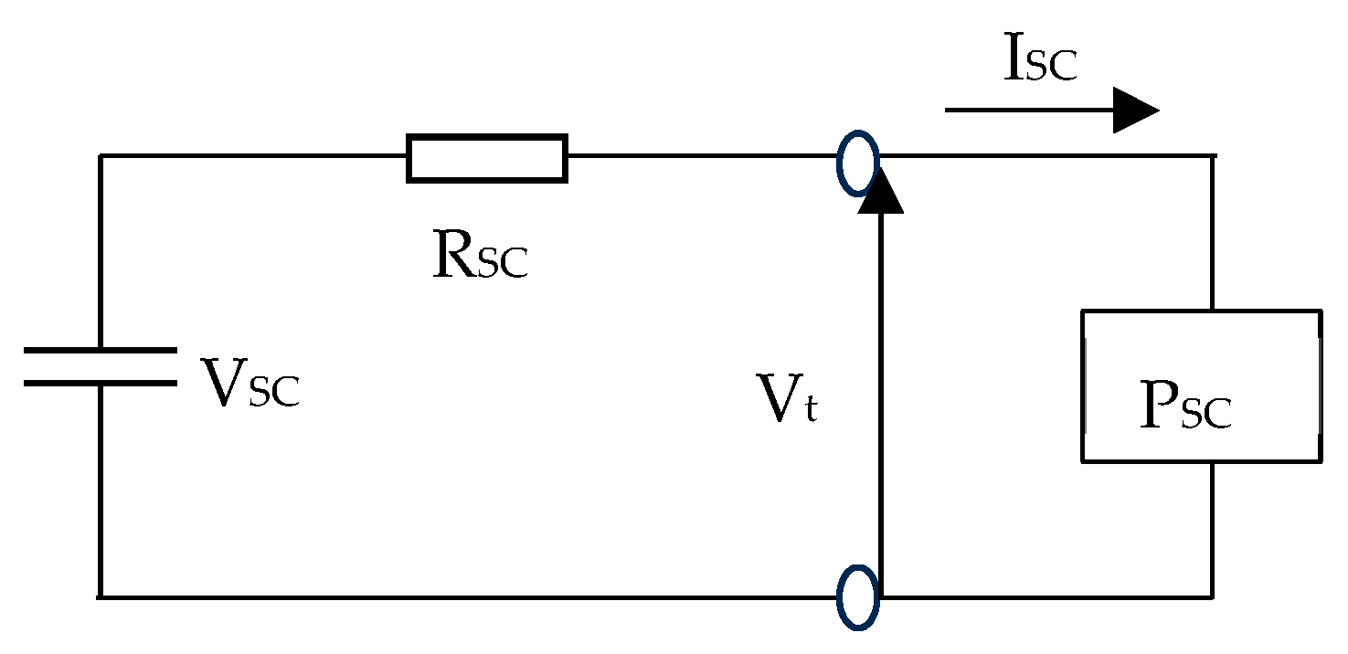
2.4. Supercapacitor Modeling

As mentioned earlier, different types of BTs and SCs were used to show the viability of the proposed ESS sizing methodology in working with different types of power sources.
Regarding SCs, the dual-layer electrochemical capacitor technology presents itself as the best alternative to use SCs as power sources in EVs [15]. Therefore, we chose two Maxwell SC types in this study.
The same equivalent circuit was assumed for SC modeling, as shown in Figure 4. RSC is the internal resistance, VSC is the nominal voltage, ISC is the current, Vt is the supply voltage, and PSC is the power required or supplied to the supercapacitors.
Equation (19) describes the SC’s terminal voltage as a function of the VSC’s nominal voltage and the power PSC.
V t = V S C + V S C 2 4 R S C P S C / 2 .
The energy stored in SCs, ESC, and the energy removed in the nth simulation step are in Equations (23) and (24), respectively.
E S C = 1 / 2 C   V S C 2
E S C   n + 1 = E S C   n δ t × V S C I S C ,
where C is the nominal capacity and δt is the time interval in seconds between sequential computations.
Moreover, the SC estate of charge, SoCSC, is given by Equation (25) [46]:
S o C S C = V S C / V S C   m a x 2
Data used in SC modeling are in Table 3.

3. Methodology

In this section, the enveloped power profile, obtained by overlapping the power demand profiles of five driving cycles, is shown. Subsequently, the coefficients of the sources’ specific energy and power (BTs and SCs) are presented using the respective Ragone plots. Then, the methodology to size the ESS is introduced. Finally, the power and the energy management strategy are described.

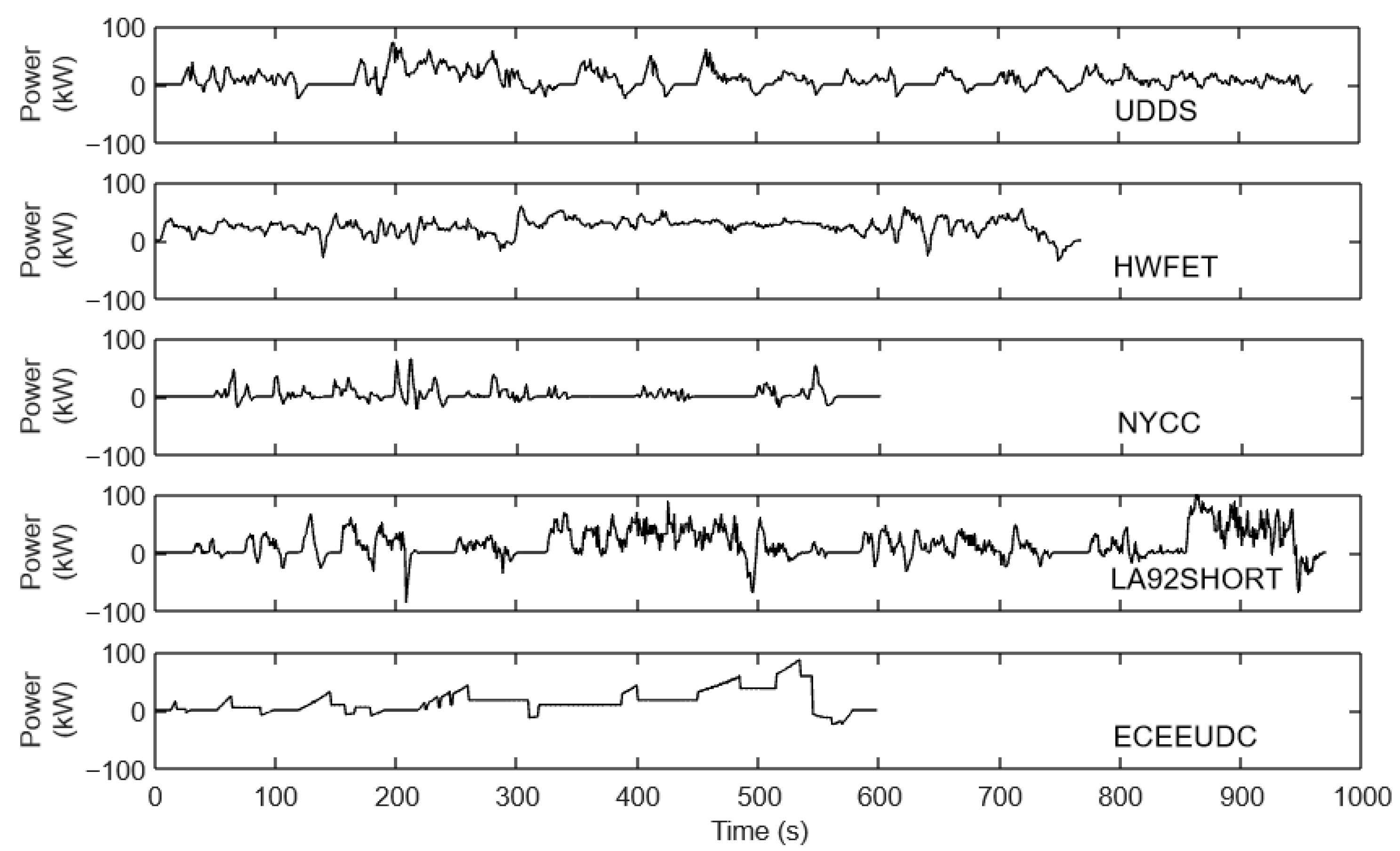
3.1. Driving Cycles Used in the ESS Sizing Methodology

It is considered the use of different driving cycles in order to cover the most varied driving conditions that the vehicle can be subject to, e.g., frequent stop-and-go and high cruising speeds. Therefore, the ESS should have sufficient energy and power capacities to drive the vehicle in different conditions. These driving cycles are shown in Figure 5 [49]. Three of them depict urban driving conditions: the Urban Dynamometer Driving Schedule (UDDS), the New York City Cycle (NYCC), and the Elementary Urban Cycle added to the Extra-Urban Driving Cycle (ECEEUDC). The other two driving cycles regard highway driving conditions: the LA92Short, whose first 969 s belong to the Unified Dynamometer Schedule, and the Highway Fuel Economy Driving Schedule (HWFET). All driving cycles are shown in 1000 s.

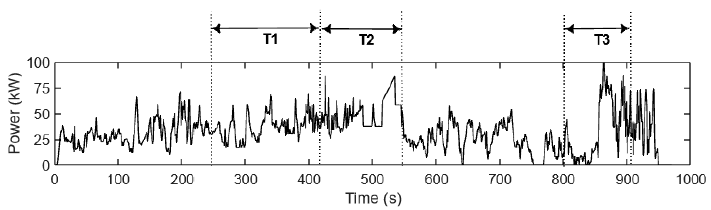
3.2. Envelope Power Profile

To determine an ESS sizing consistent with the unpredictability of the power demand, we devised a power profile to represent random drivability conditions. Such a power profile is an envelope type that was obtained by overlapping the profiles of the driving cycles, depicted in Figure 6. We investigate configurations with minimum ESS mass, able to deliver power peaks with no participation of the autonomy source.
Figure 7 shows the intervals of the enveloped power profile used in the ESS sizing methodology. These intervals are between 288 and 433 s (T1), 433 and 585 s (T2), and 840 and 950 s (T3).
The power peaks are more frequent in the selected intervals than in the remaining envelope. Soon, the ESS sizing methodology was applied to each interval, resulting in different ESS sizes.
The methodology considers only the positive part of the power envelope, as in Figure 7. In actual driving conditions, the braking power is not predictable and, in magnitude, is generally higher than the acceleration. The negative power relates to breaking intervals and affects the vehicle’s autonomy, not the power demand. In this study, when the charge limit of the ESS overflows, the mechanical brakes are engaged.

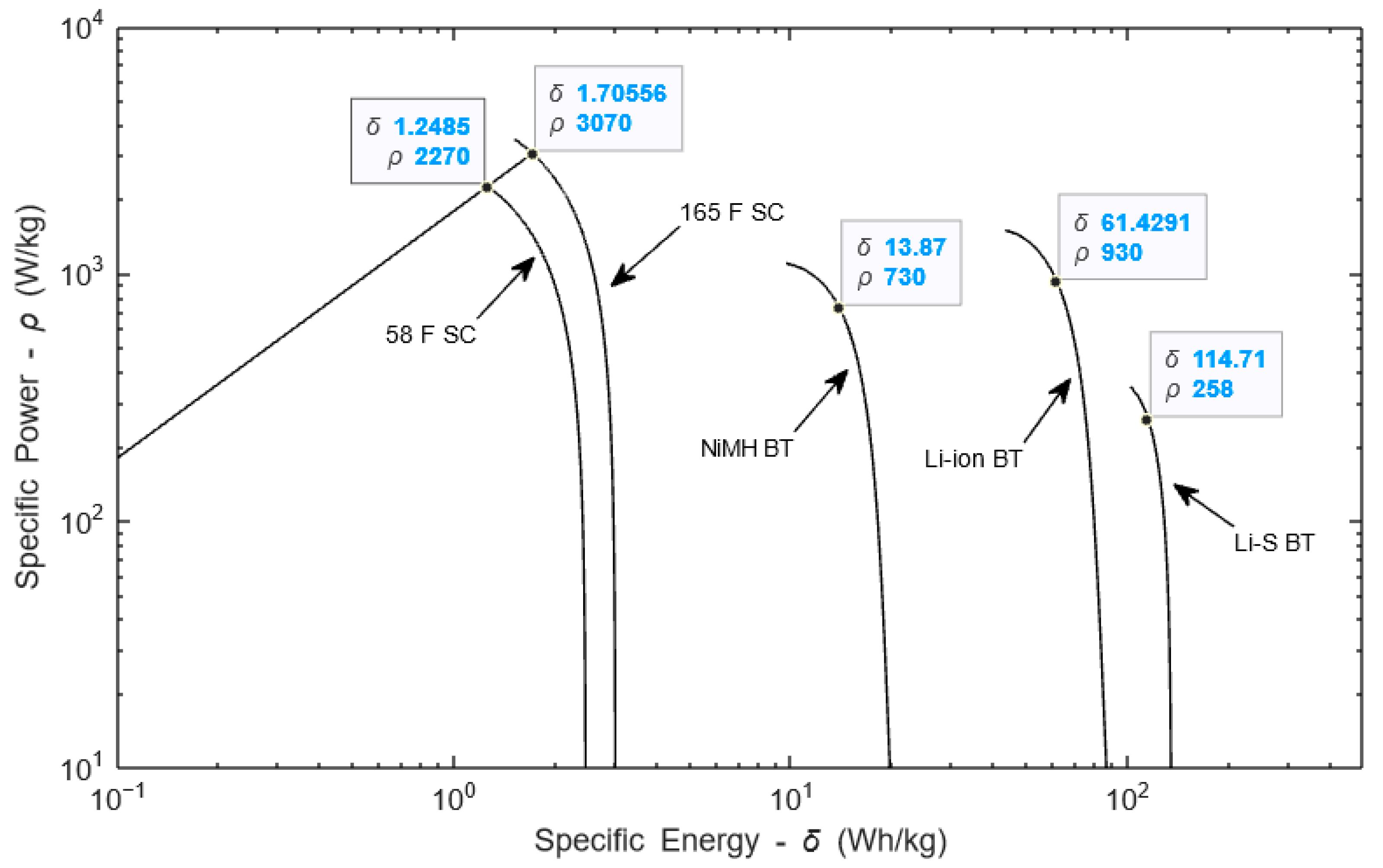
3.3. Ragone Coefficients

The Ragone plot provides information about the energy and power in the power sources [11,12]. The sizing methodology detailed description of how the Ragone plots were obtained in Figure 8 is given in [2].
The coefficients of specific energy δ and specific power ρ should be as large as possible to obtain an ESS of low mass. As can be seen in Figure 8, on the curved path, the specific energy and power coefficients are high. These high values of coefficients are depicted in blue for each BT and SC type. The sizing methodology will only add a new string of BTs or SCs if the previous ones cannot comply with the pre-established operating limits.
The SCs must operate in a region where they deliver maximum power in two seconds. In this case, despite the high values, 1.255 W/kg and 2260 Wh/kg for the 58 F SC, and 1.706 W/kg and 3070 Wh/kg for the 165 F SC, these values are in a safe region. These coefficients were taken from the intersection between the straight line of two seconds and the SC’s Ragone plots (see Figure 8).
In Figure 8, the straight line of two seconds does not intersect the BT’s Ragone plots; this means that the SCs are more efficient in delivering their available power in short periods and BTs in long periods. Because of the high values of the power and energy coefficients for these SCs, the sizing methodology will allocate the power peaks to them and not to BTs. This characteristic saves the BTs from high power peaks, contributing to extending their service life.
Figure 8 allows us to demonstrate that if a single power source cannot meet the power requirement of an application, a hybrid ESS can offer a significant solution.
For the BTs, the criterion to determine the energy and power density coefficients was the same as that used in [12]. In this case, the power capacity was considered the limiting factor for BT sizing.
It was assumed that the BTs operated with an efficiency, ƞBT, higher than 80%. This value was obtained by the ratio between the power demand and the BTs’ available power, Pbat, with no internal resistance. Hence, these BT coefficients ensure that they operate with an efficiency of at least 80%. Then, the coefficients of the BTs, presented in Figure 8, were obtained by Equation (26):
δ W h / k g = ρ W / k g t 3600 .
In this figure, the coefficients of specific energy are on the x-axis and are represented by X, and the coefficients of specific power are on the y-axis and are represented by Y. In this study, for each BT/SC type, the coefficients of particular energy and power are in the most efficient curved path. For each source, in the sequence of 58 F SC, 165 F SC, NiMH BT, Li-ion BT, and Li-S BT, their coefficients of specific energy and power are 1.248 and 2270, 1.706 and 3070, 13.87 and 730, 61.43 and 930, 114.7 and 258, in Wh/kg and W/kg, respectively.

3.4. Optimization Problem—ESS Sizing Methodology

The optimal sizing based on non-linear optimization has been frequently used [10,12,15,50,51].
The objective function is
M E S S = n B T   m B T + n S C   m S C ,
where nBT and nSC are the number of strings of BTs/SCs connected in parallel. The number of cells or packs connected in series for BTs and SCs is fixed. mBT and mSC are the mass of one BT/SC string. These values are summarized in Table 4.
Now, the constraints for the optimization problem are the following:
  • The power required of the envelope power profile (Figure 7) is equal to the power delivered by the ESS, PESS, plus the power produced by the autonomy source, Pautonomy:
P r e q = P E S S + P a u t o n o m y .
We aimed to find the optimal ESS sizing to meet the high power interval required without the autonomy source’s participation. Consequently, the power demand during the selected intervals (T1, T2, or T3) equals the power the ESS requires.
P r e q = P E S S ,
P E S S = P B T + P S C ,
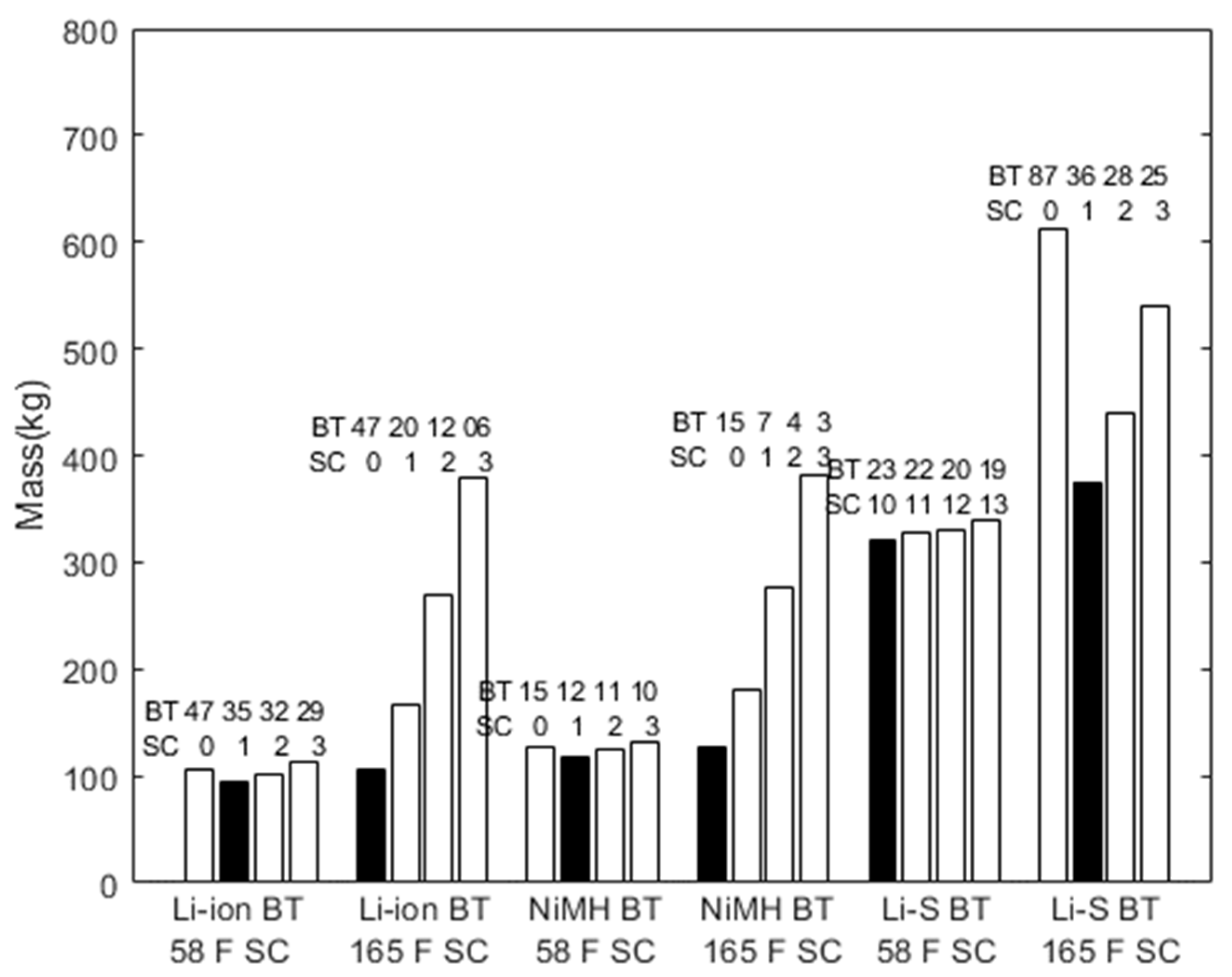
  • The ESS power cannot exceed the maximum available power in the BT and SC strings. This available power was estimated considering the coefficients of maximum specific power, ρBT, ρSC, taken from the BT’s/SC’s Ragone plots in Figure 8.
P B T ρ B T   n B T   m B T P S C ρ S C   n S C   m S C
  • The SC voltage is between Vtmax (400 V) and Vtmin (250 V):
V t m a x V t V t m i n
This constraint works with the SC model described in Section 2.4.
  • The BT state of charge, between the maximum, SoCBTmax (100%), and the minimum, SoCBTmin (60%), values is as follows:
S o C B T m a x S o C B T S o C B T m i n
Because of the high power density of the SCs, the methodology allocates the power peaks to them and not to the BTs, contributing to extending the BT’s service life.
In summary, the ESS sizing methodology finds nBT, nSC, PBT, and PSC as the variables that minimize the objective function in Equation (27).
The algorithm was performed in the fmincon routine, present in the Matlab/Simulink optimization toolbox. This routine uses the Quasi-Newton method for constrained optimization, known as Quadratic Sequence Programming [52].

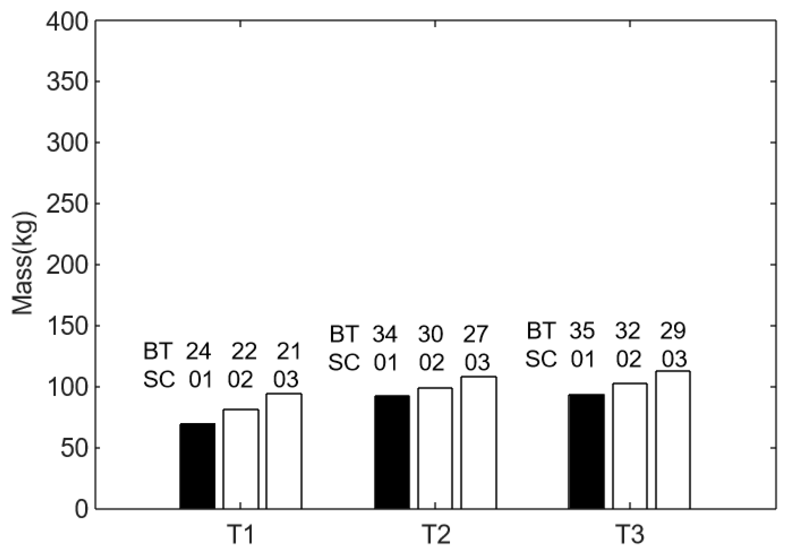
3.4.1. ESS Sizing Methodology Input Data

The vector (x0) contains the input data of the optimization problem variables: the initial number of BT and SC strings, nBTi and nSci, respectively; PBTi and PSCi are the initial vectors of BT/SC power required.
x 0 = n B T i , n S C i , P B T i , P S C i
nBTi and/or nSCi are always updated; PBTi is updated according to Equation (35) and represents the maximum power which the BT bank can deliver, PBTimax:
P B T i m a x = n B T i   m B T   ρ B T ,
where mBT and ρBT are taken from Table 2.
The update of PBTi and PSCi is necessary to generate feasible inputs to the optimization algorithm.
Figure 9 shows the interval T3 used in the ESS sizing methodology. The power demand depicted in this figure is PESS. Therefore, according to the power balance equation, PSCi is as follows:
P S C i = P E S S P B T i
According to Figure 9,
P E S S P B T i m a x ,   P B T i = P E S S   a n d   P S C i = 0 P E S S > P B T i m a x ,   P B T i = P B T i m a x   a n d   P S C i = P E S S P B T i

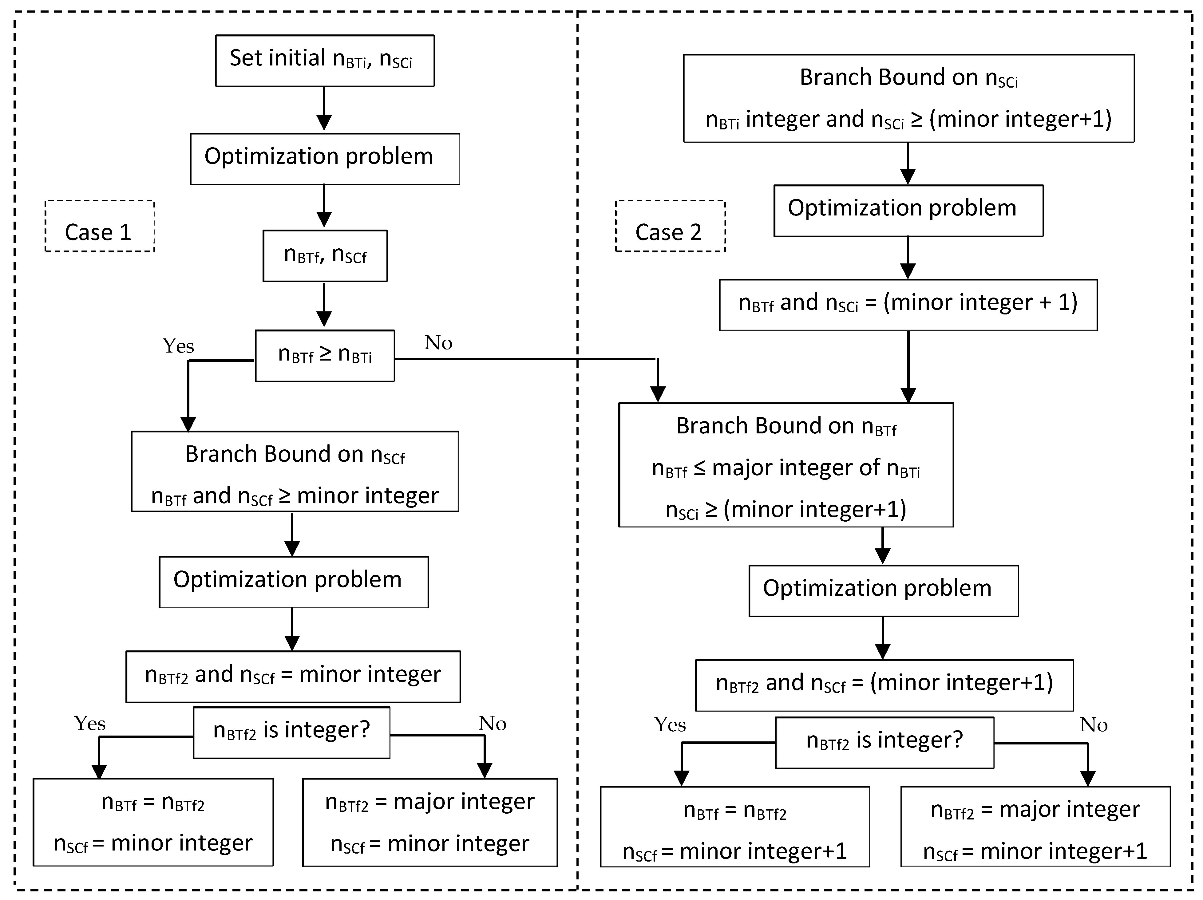
3.4.2. ESS Sizing Methodology Overview

Figure 10 depicts the steps to proceed with the ESS sizing methodology. The top of this figure shows the power profiles of the driving cycles (a) in Section 3.2, that were used to compose the envelope power profile (b). Block (c) contains the six ESSs types of configurations that the sizing methodology can handle with: ESS1, with Li-ion BTs and 58 F SCs; ESS2, with Li-ion BTs and 165 F SCs; ESS3, with NiMH BTs and 58 F SCs; ESS4, with NiMH BTs and 165 F SCs; ESS5, with Li-S BTs and 58 F SCs; and ESS6, with Li-S and 165 F SCs. Once an ESS configuration has been chosen, (d), for example, ESS1, the inputs of the sizing model are relative to that configuration, (e). In other words, for ESS1, x0, mBT, and mSC are the input vector detailed in Section 3.4.1, the mass of one string of Li-ion BT, and the mass of one string of 58 F SC, respectively (see Table 4). The block (f) summarizes the sizing methodology developed as an optimization problem. This block divides the constraints of the method into linear, (30) and (31), and non-linear, (32) and (33), constraints. We can see that the non-linear constraints depend on the BT and SC models developed in Section 2.3 and Section 2.4. Lastly, (g) shows the types of results that the ESS sizing methodology can offer: the configuration of ESS1 of low mass and all the possibilities of configurations of ESS1 of low mass for a fixed number of nSC1. The way these results were obtained is explained further, in Section 4.1.

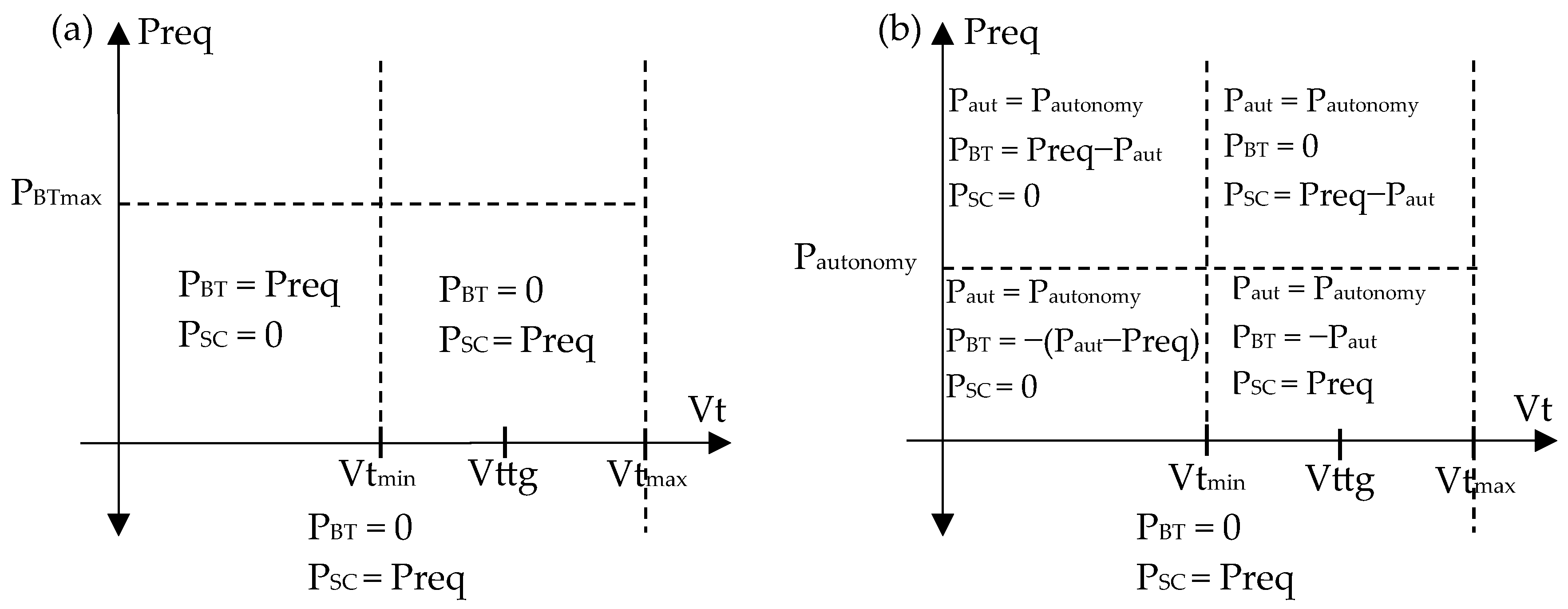
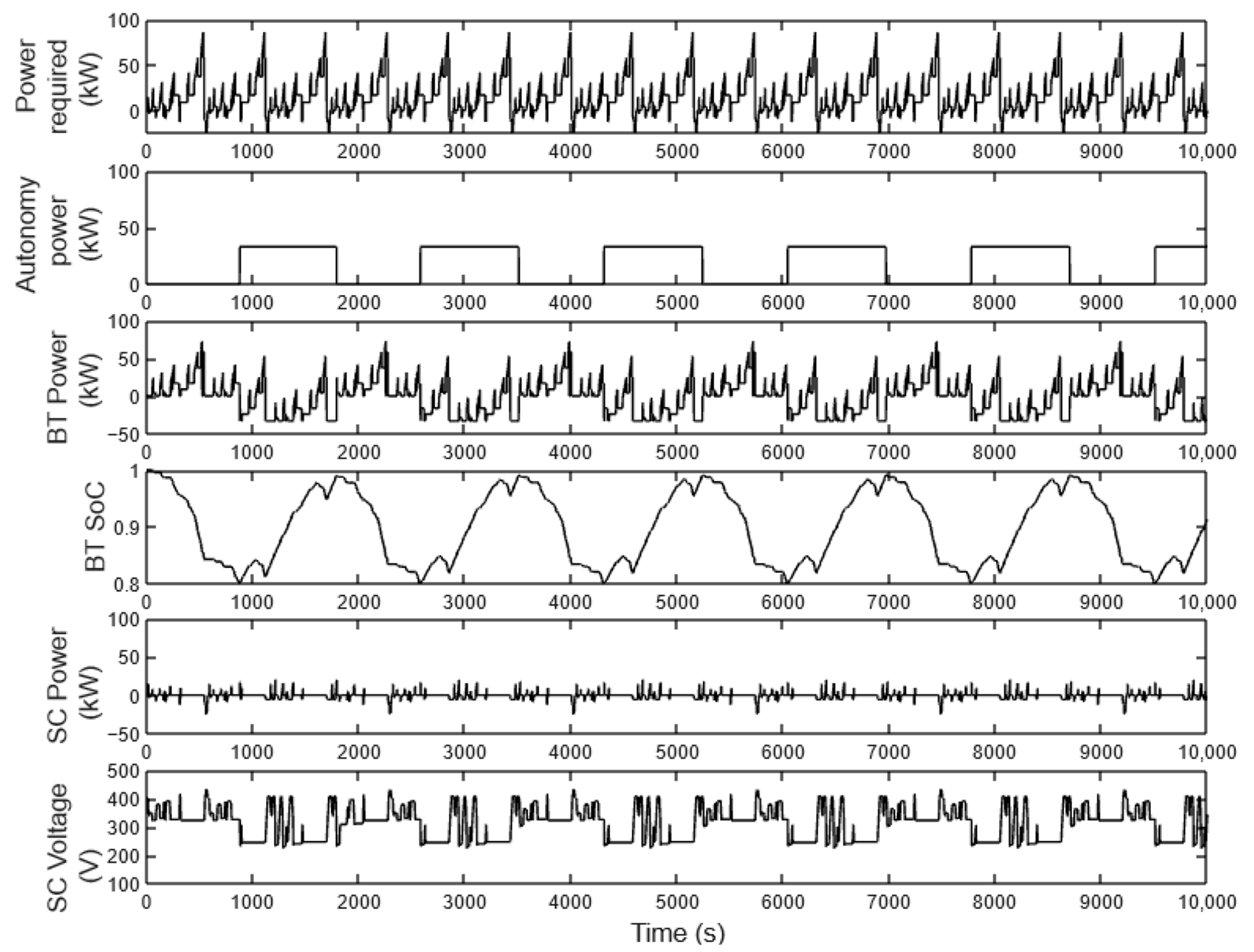
3.5. Rules-Based Energy Management

Previous studies [10,15,53,54,55] have pointed out control strategies based on deterministic rules to control the power flow among different power sources in EVs. The rules described below are based on the SoCBT and the battery bank’s maximum power. Since batteries can account for up to 40% of the cost of an EV, it is essential to ensure that they work within their operational limits. The power demanded from the battery pack should be less than its maximum value, PBTmax. The SC bank plays an important role in quickly processing the power required during fast acceleration and braking, while the BTs are controlled to respond slowly.
Therefore, the rules of the energy management strategy are as follows:
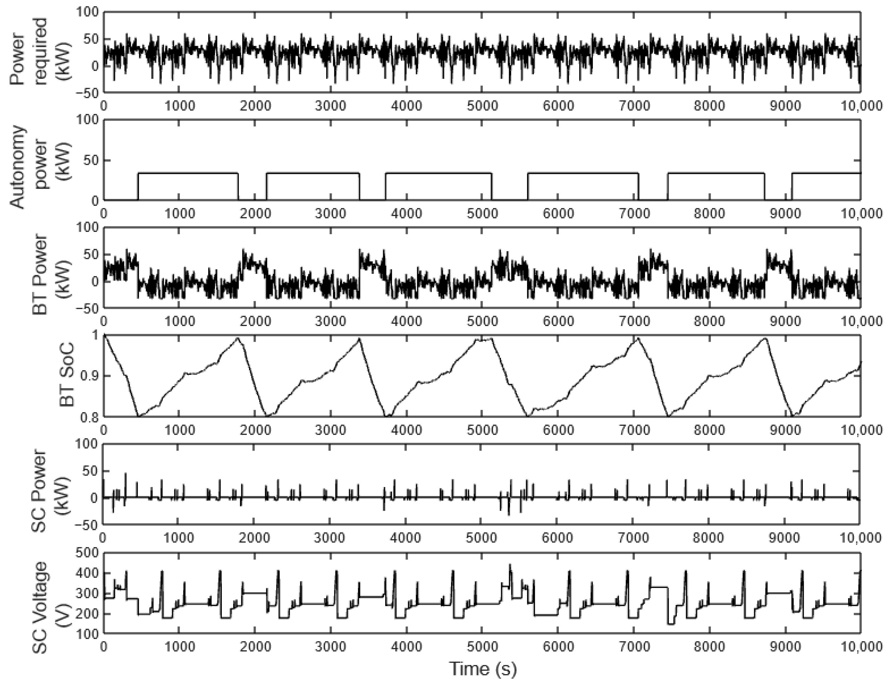
  • Power deliverable by the autonomy source must be equal to the average power of the envelope power profile in Figure 7, i.e., 33 kW.
  • The autonomy source has an on/off control. When PBTmax is reached, the autonomy source is turned on to provide a power system, reducing the BT demand. Once SoCBTmax is reached, the autonomy source is turned off.
  • The SC voltage should be kept around its half load (Vttg ≈ 330 V). At this voltage, the SC can provide extra power in acceleration or accept power from regenerative braking. The voltage regulation is controlled via the BT bidirectional converter.
  • The SC absorbs the regenerative braking energy.
Energy management considers the maximum value of the power required from the BT, PBTmax, the power needed for the vehicle, Preq, and the SC voltage as limiting factors.
As shown in Figure 11, the energy management rules are displayed in two Cartesian planes regarding the autonomy source’s state (on/off). Figure 11a displays the rules when the autonomy source is turned off, and Figure 11b displays the rules when the autonomy source is turned on. When SoCBTmax is reached, the energy management works with the rules in Figure 11a. When Preq > PBTmax, the energy management works with the rules in Figure 11b.

4. Results and Discussion

The present study was performed by considering three types of BTs: Li-ion, NiMH, and Li-S, and two values of SCs: 58 F and 165 F. Hence, we have six ESS configurations (BT/SC): Li-ion/58 F (ESS1), Li-ion/165 F (ESS2), NiMH/58 F (ESS3), NiMH/165 F (ESS4), Li-S/58 F (ESS5), and Li-S/165 F (ESS6). Different types of BTs and SCs were used to show the viability of the proposed ESS sizing methodology, based on non-linear optimization, with varying power sources.
After obtaining the local optimal ESS sizing for each of the selected time intervals, it is possible to find the global optimal ESS sizing with the minimum mass.
Figure 12 presents the three best results for ESSs with Li-ion BTs and 58 F SCs for each selected time interval. The ESS of the lowest mass corresponds to T1. This ESS weighs 69.75 kg and has 24 Li-ion BTs strings and one 58 F SCs. On the other hand, the ESS of the biggest mass regards T3, with 113 kg, 29 strings of Li-ion BTs, and three strings of 58 F SCs.
As shown in Figure 12, heavy ESSs are found for T3, which denotes that this is the interval with higher power demand. This means the lighter ESS could not deliver the required power in the T3 interval. Consequently, the selected ESS weighs 93.7 kg and has 35 strings of Li-ion BTs and one string of 58 F SCs.
Figure 13 shows the four best optimal ESSs for the six ESS configurations for the interval T3. The values that align with BT/SC represent the number of strings of BTs or SCs.
The Li-ion/58F ESS (35 strings of Li-ion BTs and one string of 58 F SC) has 93.7 kg, while the heavier Li-ion/58F ESS (three strings of 58 F SC and 29 strings of Li-ion BTs) has 113 kg. This 19 kg difference can be ignored if the price and/or availability of SCs prove to be more advantageous than those for batteries. In this case, the methodology proved to be quite efficient in obtaining the smallest number of BT strings for a fixed number of SC strings.
As can be seen in Figure 13, the ESSs Li-ion/58 F and NiMH/58 F have similar masses. The NiMH/58 F ESS mass is 25 kg above the Li-ion/58 F mass.
Each string of 165 F SC adds 121 kg to the ESS vs. 2.25 kg of the Li-ion BT string, explaining why the solutions with this SC are not the best with Li-ion and NiMH.
On the other hand, the 58 F SC string is 15.75 kg, still heavier than the Li-ion string. However, the higher power density makes the combination of 58 F SC with the Li-ion BT lighter. The high-power capacity of the 58 F SC compensates for its mass. This analysis can be extended also to NiMH and Li-S batteries.
For the Li-S BTs solutions, the high number of strings of 58 F SC (10 or more) is explained by the low power capacity of the Li-S BTs (258 W/kg in this analysis). In this case, the 165 F could be considered competitive.
Despite the differences between the methodology presented in this work and the methodologies presented in [2,12], some comparisons are possible. Regarding the types of BTs and SCs, all these works agreed that a hybrid ESS is more advantageous than an ESS with BTs or SCs.
The ESSs mass found by [2,12] is 159 kg and 200 kg, respectively. However, these mass values are larger than those found now (94.7 kg). Such a difference is because we have not considered the addition of the mass necessary for the balancing and packaging of the battery cells. Such consideration could double the value of the battery cell mass, which may change the result. However, the methodology easily allows the inclusion of the additional mass in the calculations.
The nominal power of the autonomy source in those works was 70 kW vs. the 33 kW obtained with the proposed procedure.

4.1. Simulation Procedure

Initially, simulations are started with random inputs of BT and SC strings. For example, for ESSs with Li-S BTs and 58 F SCs, the initial quantities are 15 BT strings and 20 SC strings, and the final values achieved for these inputs are 26 BT strings and 9.58 SC strings.
Then, the following simulation starts with 26 and 10 strings, respectively, resulting in 24 and 9.4 BT and SC strings.
The sizing methodology routine provides similar results for different inputs. These close results indicate that the global minimum is, at least, near them.
To achieve an integer number of SC strings and the minimum number of BT strings, the following simulation starts with the previous result, i.e., 24 and 9.4 of BT and SC strings, respectively. For each minimum local found, at least one string of SC is taken off or added, and the number of BT strings is checked out. If adding an SC string increases the mass, an SC string is removed in the following simulation, and the mass is checked out. Consequently, some local optimal result around the best is obtained.
Table 5 summarizes the steps to find the size of the two ESSs of minimum mass, as in Figure 13, for the combinations of Li-ion BTs and 58 F SCs.
Each row has the initial and the final (output) number of BT and SC strings.
In the cases analyzed in Table 5, the Branch-and-Bound method is applied to the number of SC strings (second row of Cases 1 and 2). Next, the resulting number of BT strings is increased (third row of Cases 1 and 2). As reported, the Branch-and-Bound algorithm [52] is applied in the constraint of (28) to give integer numbers of BT/SC strings.
In the second row of “Case 1”, we see that the final value obtained in the previous simulation is used as the input data for the number of BT strings. The Branch-and-Bound method is applied to the number of SC strings.
In the second row of “Case 2”, the Branch-and-Bound method is also applied to the number of BT strings because the BT input data, 32.87, gave an infeasible result in the earlier attempt. Therefore, the Branch-and-Bound method is applied to the number of BT strings to limit the algorithm action.
Figure 14 shows the steps taken in Cases 1 and 2.

4.2. Rule-Based Energy Management

In this section, we use the energy management strategy to investigate the power flow between the ESS devices and the autonomy source.
These simulations are performed for the ESS with 35 strings of Li-ion BTs and one string of 58 F SCs, and the BTs and SCs are fully charged.
The autonomy source power is the average power of the envelope power profile, i.e., 33 kW, and this source is turned on or off depending on the conditions of the ESS devices. The autonomy source is turned on when the limit PBTmax or SoCBTmin is reached. Once SoCBTmax is reached, the autonomy source is turned off.
All simulations analyze 10 thousand seconds (nearly three hours). Figure 15 shows the power demand, the autonomy source operation, and the ESS main variables. There are 13 repetitions of the HWFET driving cycle. After being turned on, the autonomy source works for around 20 to 24 min. This time interval is appreciably longer than those observed for the other driving cycles, such as 500 s for the NYCC driving cycle. Given the features of a highway, with speeds around 100 km/h most of the time, the HWFET driving cycle presents a high value of average power demand, 24 kW, consistent with the operation of the autonomy source.
The ECEEUDC driving cycle, as shown in Figure 16, has a power peak of 100 kW. The autonomy source remains turned on for 900 s, less than that observed for HWFET since the average power is lower, at 15 kW. Hence, it can be assumed that the operation of the autonomy source does not depend on the power peak.
The frequency of the switching behavior observed in the autonomy source depends on the limit value of the BT SoC. Reducing the limit, the off and the on intervals increase, reducing the switching frequency.

4.3. A Brief Analysis of ESS’s Cost

The algorithm was developed targeting the ESS’s minimum mass. However, the resulting ESS combination may need to be more economically viable. The total cost of these sources, whether the acquisition cost, operation cost (cost per cycle), or durability and maintenance costs, is of great importance in the sizing of a hybrid ESS [56].
From a brief analysis, the purchase costs can be analyzed in terms of wholesale and retail costs. The more units are purchased, the cheaper it is, and vice versa. On the other hand, the operating cost, which is the cost per cycle of charge and discharge of the battery, will be lower the greater the number of the target cycles. Furthermore, durability and maintenance also add costs to the total cost depending on the type of battery chosen.
We have decided not to delve into the cost issue because this analysis strongly depends on the location where these sources are intended to be purchased, and prices vary significantly from one country to another [57,58]. An operational cost analysis also depends on the location where the vehicle will be used since the energy cost changes.
Given these considerations, a case study that considers the issue of the total cost in a sizing problem needs the following:
For retail or wholesale costs, the following are needed:
  • The definition of the location.
  • Types and models of batteries available.
For operating cost, the following are needed:
  • Definition or estimation of where and how the vehicle will be driven.
  • Considering sizing and management, how many cycles can these batteries withstand?
  • The local energy and fuel costs.
In the present work, regarding battery life, both sizing and management ensure that the battery bank will not deliver power above its maximum limit. The management strategy ensures this. Furthermore, the autonomy source recharges the battery bank, allowing accurate and safe control.

5. Conclusions

The ESS sizing methodology searches for minimum mass solutions and is able to comply with the enveloped power demand without participating in the autonomy source.
Although the proposed ESS sizing methodology can find the local minima, it is impossible to guarantee that it is the global minimum. The possibility of finding local minima is an advantage because they represent all possible configurations of ESS lower mass that are capable of meeting the power demand.
All the ESS configurations associated with the local minima meet the constraints stated for the ESS sizing methodology. These constraints mainly consider a safe region of operation for the sources. This task is ensured by power limits, set by the power coefficients ρBT and ρSC, and BT SoC and SC voltage limits. Regarding the BTs’ service life, the sizing methodology works to extend them because, beyond the limits listed in the constraints, the response for power peaks is in charge of the SCs.
This methodology can be applied to other sources or ESS configurations beyond those analyzed in this work, as long as they fit into the models presented and to any power demand profile. For example, someone may want to use two or more types of batteries, either without or with supercapacitors. The fact that this methodology applies to intervals of time-varying power demand makes the sizing of the sources more robust despite being minimal in mass. The methodology can be easily adjusted to other vehicle types, such as buses or microbuses.
Future work on source sizing should include the lifetime of the sources since different numbers of BTs/SCs strings can affect the system’s lifetime, i.e., ESS configurations that can also maximize the service life of the system and, consequently, the EV range, reducing the source’s maintenance and replacement cost.

Author Contributions

Conceptualization, J.A.P. and P.A.V.F.; methodology, P.A.V.F.; software, J.L.; validation, J.L.; formal analysis, J.L. and J.A.P.; investigation, J.L.; resources, J.A.P.; data curation, J.L. and J.A.P.; writing—original draft preparation, J.L.; writing—review and editing, J.L. and J.A.P.; visualization, J.L. and J.A.P.; supervision, J.A.P. and P.A.V.F.; project administration, J.A.P.; funding acquisition, J.A.P. All authors have read and agreed to the published version of the manuscript.

Funding

This work was partly supported by the Sao Paulo Research Foundation under grant #2008/01162-6 and Brazilian National Research Council, #303859/2020-2.

Data Availability Statement

The raw data supporting the conclusions of this article will be made available by the authors on request.

Conflicts of Interest

The authors declare no conflict of interest.

References

  1. Koengkan, M.; Fuinhas, J.A.; Teixeira, M.; Kazemzadeh, E.; Auza, A.; Dehdar, F.; Osmani, F. The Capacity of Battery-Electric and Plug-in Hybrid Electric Vehicles to Mitigate CO2 Emissions: Macroeconomic Evidence from European Union Countries. World Electr. Veh. J. 2022, 13, 58. [Google Scholar] [CrossRef]
  2. Lopes, J.; Pomílio, J.A.; Ferreira, P.A.V. Optimal Sizing of Batteries and Ultracapacitors for Fuel Cell Electric Vehicles. In Proceedings of the IECON 2011—37th Annual Conference of the IEEE Industrial Electronics Society, Melbourne, Australia, 7–10 November 2011. [Google Scholar]
  3. Gurkaynak, Y.; Khaligh, A.A.; Emadi, A. State of the Art Power Management Algorithms for Hybrid Electric Vehicles. In Proceedings of the IEEE Vehicle Power Propulsion Conference, Dearborn, MI, USA, 7–10 September 2009. [Google Scholar]
  4. Li, M.; Xu, H.; Li, W.; Liu, Y.; Li, F.; Hu, Y.; Li, L. The Structure and Control Method of Hybrid Power Source for Electric Vehicle. Energy 2016, 112, 1273–1285. [Google Scholar] [CrossRef]
  5. Thounthong, P.; Raël, S.; Davat, B. Energy Management of Fuel Cell/Battery/Supercapacitor Hybrid Power Source for Vehicle Applications. J. Power Sources 2009, 193, 376–385. [Google Scholar] [CrossRef]
  6. Mahmoudi, C.; Flah, A.; Sbita, L. An overview of electric vehicle concept and power management strategies. In Proceedings of the International Conference on Electrical Sciences and Technologies in Maghreb, Tunis, Tunisia, 3–6 November 2014. [Google Scholar]
  7. Becker, J.; Schaeper, C.; Sauer, D. Energy management system for a multi-source storage system electric vehicle. In Proceedings of the IEEE Vehicle Power Propulsion Conference, Seoul, Republic of Korea, 9–12 October 2012. [Google Scholar]
  8. Liu, F.; Wang, C.; Luo, Y. Parameter Matching Method of a Battery-Supercapacitor Hybrid Energy Storage System for Electric Vehicles. World Electr. Veh. J. 2021, 12, 253. [Google Scholar] [CrossRef]
  9. Larminie, J.; Lowry, J. Electric Vehicle Technology Explained; John Wiley & Sons Ltd.: Chichester, UK, 2003; ISBN 0-470-85163-5. [Google Scholar]
  10. Lopes, J. Optimal Sizing and Power Management Methodologies of Energy Sources for Electric Vehicles. Available online: http://repositorio.unicamp.br/bitstream/REPOSIP/260868/1/Lopes_Juliana_D.pdf (accessed on 2 July 2019).
  11. Christen, T.; Carlen, M.W. Theory of Ragone Plots. J. Power Sources 2000, 91, 210–216. [Google Scholar] [CrossRef]
  12. Schupbach, R.; Balda, J.; Zolot, M.; Kramer, B. Design Methodology of a Combined Battery-Ultracapacitor Energy Storage Unit for Vehicle Power Management. In Proceedings of the IEEE 34th Annual Conference on Power Electronics Specialist, Acapulco, Mexico, 15–19 June 2003. [Google Scholar]
  13. Tu, J.; Bai, Z.; Wu, X. Sizing of a Plug-In Hybrid Electric Vehicle with the Hybrid Energy Storage System. World Electr. Veh. J. 2022, 13, 110. [Google Scholar] [CrossRef]
  14. KoteswaraRao, K.V.; Srinivasulu, G.N.; Rahul, J.R.; Velisala, V. Optimal component sizing and performance of Fuel Cell—Battery powered vehicle over world harmonized and new european driving cycles. Energy Convers. Manag. 2024, 300, 117992. [Google Scholar] [CrossRef]
  15. Bauman, J.; Kazerani, M. A Comparative Study of Fuel-Cell–Battery, Fuel-Cell–Ultracapacitor, and Fuel-Cell–Battery–Ultracapacitor Vehicles. IEEE Trans. Veh. Technol. 2008, 57, 760–769. [Google Scholar] [CrossRef]
  16. Huilong, Y.; Cao, D. Multi-objective Optimal Sizing and Real-time Control of Hybrid Energy Storage Systems for Electric Vehicles. In Proceedings of the IEEE Intelligent Vehicle Symposium, Changshu, China, 26–30 June 2018. [Google Scholar]
  17. Araújo, R.E.; Castro, R.; Pinto, C.; Melo, P.; Freitas, D. Combined Sizing and Energy Management in EVs With Batteries and Supercapacitors. IEEE Trans. Veh. Technol. 2014, 63, 3062–3076. [Google Scholar] [CrossRef]
  18. Souffran, G.; Miegeville, L.; Guerin, P. Simulation of Real-World Vehicle Missions Using a Stochastic Markov Model for Optimal Powertrain Sizing. IEEE Trans. Veh. Technol. 2012, 61, 3454–3465. [Google Scholar] [CrossRef]
  19. Schwarzer, V.; Ghorbani, R.; Rocheleau, R. Drive cycle generation for stochastic optimization of energy management controller for hybrid vehicles. In Proceedings of the IEEE International Control Applications Conference, Yokohama, Japan, 8–10 September 2010. [Google Scholar]
  20. Banvait, H.; Anwar, S.; Chen, Y. A rule-based energy management strategy for Plug-in Hybrid Electric Vehicle (PHEV). In Proceedings of the American Control Conference, St. Louis, MO, USA, 10–12 June 2009. [Google Scholar]
  21. Wu, J.; Peng, J.; He, H.; Luo, J. Comparative Analysis on the Rule-based Control Strategy of Two Typical Hybrid Electric Vehicle Powertrain. Energy Procedia 2016, 104, 384–389. [Google Scholar] [CrossRef]
  22. Gillespie, T. Fundamentals of Vehicle Dynamics; SAE International: Warrendale, PA, USA, 1992; ISBN 978-1-4686-0176-3. [Google Scholar]
  23. Ulitskaya, J. Which Electric Vehicles Are Most Available Right Now? Available online: https://www.cars.com/articles/which-electric-vehicles-are-most-available-right-now-448044/ (accessed on 23 January 2023).
  24. Goodwin, A. Best Electric Cars and EVs for 2024. Available online: https://www.cnet.com/roadshow/news/best-ev-electric-car/ (accessed on 23 January 2023).
  25. Best Electric Cars. Available online: https://www.truecar.com/best-cars-trucks/cars/fuel-electric/ (accessed on 23 January 2023).
  26. Electric Vehicle Research and Development. Available online: https://afdc.energy.gov/fuels/electricity_research.html#battery (accessed on 23 January 2023).
  27. Volvo Car Group Signs Multi-Billion-Dollar Battery Supply Deals with CATL and LG Chem. Available online: https://www.media.volvocars.com/global/en-gb/media/pressreleases/252485/volvo-car-group-signs-multi-billion-dollar-battery-supply-deals-with-catl-and-lg-chem (accessed on 23 January 2023).
  28. Saw, L.; Yonghuang, Y.; Tay, A. Integration Issues of Lithium-ion Battery into Electric Vehicles Battery Pack. J. Clean. Prod. 2016, 113, 1032–1045. [Google Scholar] [CrossRef]
  29. Jaguemont, J.; Boulon, L.; Dubé, Y. A Comprehensive Review of Lithium-ion Batteries Used in Hybrid and Electric Vehicles at Cold Temperatures. J. Appl. Energy 2016, 164, 99–114. [Google Scholar] [CrossRef]
  30. Chen, M.; Ma, X.; Chen, B.; Arsenault, R.; Karlson, P.; Simon, N.; Wang, Y. Recycling End-of-Life Electric Vehicle Lithium-Ion Batteries. J. Joule 2019, 3, 2622–2646. [Google Scholar] [CrossRef]
  31. Xie, W.; Liu, X.; He, R.; Li, Y.; Gao, X.; Li, X.; Peng, Z.; Feng, S.; Feng, X.; Yang, S. Challenges and Opportunities Toward Fast-Charging of Lithium-ion Batteries. J. Energy Storage 2020, 32, 101837. [Google Scholar] [CrossRef]
  32. Zhang, J.; Zhang, L.; Sun, F.; Wang, Z. An Overview on Thermal Safety Issues of Lithium-ion Batteries for Electric Vehicle Application. IEEE Access 2018, 6, 23848–23863. [Google Scholar] [CrossRef]
  33. Batteries for Electric Vehicles. Available online: https://afdc.energy.gov/vehicles/electric_batteries.html (accessed on 23 January 2023).
  34. Torabi, F.; Ahmadi, P. Simulation of Battery Systems; Academic Press: Cambridge, MA, USA, 2020; Chapter 1; pp. 1–54. ISBN 978-0-12-816212-5. [Google Scholar]
  35. Abdin, Z.; Khalilpour, K.R. Polygeneration with Polystorage for Chemical and Energy Hubs; Academic Press: Cambridge, MA, USA, 2019; Chapter 4; pp. 77–131. ISBN 978-0-12-813306-4. [Google Scholar]
  36. Tsai, P.; Chan, L. Nickel-Based Batteries: Materials and Chemistry, Electricity Transmission, Distribution and Storage Systems; Woodhead Publishing: Sawston, UK, 2013; pp. 309–397. ISBN 978-1-84569-784-6. [Google Scholar]
  37. Ameur, A.; Berrada, A.; Loudiyi, K.; Adomatis, R. Hybrid Energy System Models; Academic Press: Cambridge, MA, USA, 2021; pp. 195–238. ISBN 978-0-12-821403-9. [Google Scholar]
  38. Merrifield, R. Cheaper, Lighter and More Energy-Dense: The Promise of Lithium-Sulphur Batteries. Available online: https://ec.europa.eu/research-and-innovation/en/horizon-magazine/cheaper-lighter-and-more-energy-dense-promise-lithium-sulphur-batteries (accessed on 23 January 2023).
  39. Patel, P. Long-lasting Lithium-Sulfur Battery Promises to Double EV Range. Available online: https://spectrum.ieee.org/lithium-sulfur-battery-news-ev-electric-vehicle-range (accessed on 23 January 2023).
  40. Lisa Project|Developing the New Generation of LIs Battery Cells. Available online: https://lisaproject.eu/ (accessed on 23 February 2023).
  41. Karthik, M.; Vijayachitra, S. Numerical Study on the Detailed Characterization of Ni-MH Battery Model for its Dynamic Behavior using Multi-Regression Analysis—MRA. IJSCE 2015, 4, 34–43. [Google Scholar]
  42. Propp, K.; Marinescu, M.; Auger, D.J.; O’Neill, L.; Fotouhi, A.; Somasundaram, K.; Offer, G.J.; Minton, G.; Longo, S.; Wild, M.; et al. Multi-Temperature State-Dependent Equivalent Circuit Discharge Model for Lithium-Sulfur Batteries. J. Power Sources 2016, 328, 289–299. [Google Scholar] [CrossRef]
  43. datasheets.com. Available online: https://www.datasheets.com/en/part-details/hhr650d-panasonic-31361681#datasheet (accessed on 3 October 2022).
  44. Kroeze, R.; Krein, P.T. Electrical battery model for use in dynamic electric vehicle simulations. In Proceedings of the IEEE Power Electronics Specialists Conference, Rhodes, Greece, 15–19 June 2008. [Google Scholar]
  45. Omar, N.; Verbrugge, B.; Mulder, G.; van den Bossche, P.; van Mierlo, J.; Daowd, M.; Dhaens, M.; Pauwels, S. Evaluation of performance characteristics of various lithium-ion batteries for use in BEV application. In Proceedings of the IEEE Vehicle Power and Propulsion Conference, Lille, France, 1–3 September 2010. [Google Scholar]
  46. Chau, K.; Wong, Y. Overview of power management in hybrid electric vehicles. Energy Convers. Manag. 2002, 43, 1953–1968. [Google Scholar] [CrossRef]
  47. maxwell.com. Available online: https://www.maxwell.com/images/documents/datasheet_16v_small_cell_module.pdf (accessed on 18 August 2019).
  48. maxwell.com. Available online: https://www.maxwell.com/images/documents/hq_48v_ds10162013.pdf (accessed on 18 August 2019).
  49. epa.gov. Available online: https://www.epa.gov/vehicle-and-fuel-emissions-testing/dynamometer-drive-schedules (accessed on 18 August 2019).
  50. Sadoun, R.; Rizoug, N.; Bartholomeüs, P.; Barbedette, B.; le Moigne, P. Optimal sizing of hybrid supply for electric vehicle using Li-ion battery and supercapacitor. In Proceedings of the IEEE Vehicle Power Propulsion Conference, Chicago, IL, USA, 6–9 September 2011. [Google Scholar]
  51. Eldeeb, H.H.; Elsayed, A.T.; Lashway, C.R.; Mohammed, O. Hybrid Energy Storage Sizing and Power Splitting Optimization for Plug-In Electric Vehicles. IEEE Trans. Ind. Appl. 2019, 55, 2252–2262. [Google Scholar] [CrossRef]
  52. Bertsekas, D.P. Nonlinear Programming; Athena Scientific: Belmont, CA, USA, 1999; ISBN 1886529051. [Google Scholar]
  53. Kouchachvili, L.; Yaïci, W.; Entchev, E. Hybrid Battery/Supercapacitor Energy Storage System for the Electric Vehicles. J. Power Sources 2018, 374, 237–248. [Google Scholar] [CrossRef]
  54. Fathabadi, H. Novel Fuel Cell/Battery/Supercapacitor Hybrid Power Source for Fuel Cell Hybrid Electric Vehicles. Energy 2018, 143, 467–477. [Google Scholar] [CrossRef]
  55. Zou, K.; Luo, W.; Lu, Z. Real-Time Energy Management Strategy of Hydrogen Fuel Cell Hybrid Electric Vehicles Based on Power Following Strategy–Fuzzy Logic Control Strategy Hybrid Control. World Electr. Veh. J. 2023, 14, 315. [Google Scholar] [CrossRef]
  56. Panaparambil, V.S.; Kashyap, Y.; Castelino, R.V. A Review on Hybrid Source Energy Management Strategies for Electric Vehicle. Int. J. Energy Res. 2021, 45, 19819–19850. [Google Scholar] [CrossRef]
  57. Global EV Outlook 2023, IEA, Paris. Available online: https://www.iea.org/reports/global-ev-outlook-2023 (accessed on 20 November 2023).
  58. Whitehead, J.; Washington, S.P.; Franklin, J.P. The Impact of Different Incentive Policies on Hybrid Electric Vehicle Demand and Price: An International Comparison. World Electr. Veh. J. 2019, 10, 20. [Google Scholar] [CrossRef]
Figure 1. Forces acting on the longitudinal movement of the vehicle.
Wevj 15 00076 g001
Figure 2. EV’s powertrain topology.
Wevj 15 00076 g002
Figure 3. Electrical circuit model for the batteries.
Wevj 15 00076 g003
Figure 4. Electrical circuit model for the supercapacitors.
Wevj 15 00076 g004
Figure 5. (ac) UDDS, NYCC, and ECEEUDC are urban driving cycles. (d,e) LA92Short and HWFET are highway driving cycles.
Wevj 15 00076 g005
Figure 6. Power required profiles of the five driving cycles in Figure 5, obtained by applying (4) to the driving cycles.
Wevj 15 00076 g006
Figure 7. Envelope power profile, obtained by overlapping the profiles of the driving cycles. Only the positive path was considered. The ESS sizing methodology uses T1–T3 periods.
Wevj 15 00076 g007
Figure 8. BTs and SCs’ Ragone plots. From left to right: Ragone plots for 58 F SC, 165 F SC, NiMH BT, Li-ion BT, and Li-S BT types.
Wevj 15 00076 g008
Figure 9. The ESS sizing methodology uses power demand during interval T3.
Wevj 15 00076 g009
Figure 10. Block diagram of the inputs needed to run the optimization problem—ESS sizing methodology. (a) power profiles of the driving cycles; (b) envelope power profile; (c) possible six ESSs types configurations; (d) chosen ESS configuration; (e) inputs for ESS1; (f) sizing methodology as an optimization problem; and (g) the sizing methodology results.
Wevj 15 00076 g010
Figure 11. Rules of energy management displayed in two Cartesian planes. The rules are presented regarding the state of the autonomy source. (a) Rules for the autonomy source turned off. (b) Rules for the autonomy source turned on.
Wevj 15 00076 g011
Figure 12. Three top local optimal ESSs sizing with Li-ion BTs and 58 F SCs for the T1, T2, and T3. The black bars show the optimal ESSs with minimum mass for Li-ion BTs and 58 F SCs: 69.75 kg, 92.25 kg, and 93.7 kg, respectively.
Wevj 15 00076 g012
Figure 13. Four top results of local optimal ESS sizing, with minimum mass, for interval T3. Black bars indicate the lighter ESS for each type.
Wevj 15 00076 g013
Figure 14. Steps taken in Cases 1 and 2.
Wevj 15 00076 g014
Figure 15. Extended HWFET driving cycle from top to bottom: power demand profile, autonomy source operation, BT power, BT SoC, SC power, and SC voltage.
Wevj 15 00076 g015
Figure 16. Extended ECEEUDC driving cycle from top to bottom: power demand profile, autonomy source operation, BT power, BT SoC, SC power, and SC voltage.
Wevj 15 00076 g016
Table 1. Values of the main parameters of the vehicle.
ParameterNomenclatureValue
Vehicle’s Gross MassM2050 kg
Vehicle’s Rotating Components’ MassMr154.8 kg
Drag CoefficientCa0.45
Vehicle’s Frontal AreaA3.16 m2
Coefficient of Rolling Resistancef0.015
Table 2. Data for BT modeling.
Manufacturer/ModelTypeTerminal Voltage [V]Capacity [Ah]Peukert CoefficientResistance [Ω]Cell Mass [kg]ρBT [W/kg]
Panasonic/CGR18650ALi-ion3.7 [44]2.2 [44]1.03 [45]Equation (18)0.045930
Panasonic/HHR650DNiMH1.26.51.0270.0020.170730
Oxis Energy pouch cellLi-S2.1141Equation (21)0.140258
Table 3. Data for SC modeling.
Manufacturer/ModelNominal
Voltage [V]
Capacitance [F]Resistance [Ω]Mass [kg]ρSC [W/kg]
Maxwell/BMOD0058 E016 B02 [47]16580.0220.632270
Maxwell/BMOD0165 P048 [48]48.61650.006313.53070
Table 4. BTs/SCs strings information.
Li-ion Li-SNiMHSC of 58 FSC of 165 F
Number of elements per string50 cells50 cells50 cells25 packsNine packs
String mass, mBT,SC (kg)2.257.058.5015.75121.5
Table 5. Steps to find the two ESSs’ sizing of lower mass for combinations with Li-ion BTs and 58 F SCs for the period T3.
nBTinSCinBTfnSCfMass (kg)
Case 123034.571.0293.85
34.57≥134.65193.71
--35194.5
Case 233≥232.872105.46
≤33≥231.552102.49
--322103.5
Disclaimer/Publisher’s Note: The statements, opinions and data contained in all publications are solely those of the individual author(s) and contributor(s) and not of MDPI and/or the editor(s). MDPI and/or the editor(s) disclaim responsibility for any injury to people or property resulting from any ideas, methods, instructions or products referred to in the content.

