Article

Visual Odometry Based on Improved Oriented Features from Accelerated Segment Test and Rotated Binary Robust Independent Elementary Features

College of Mechanical and Electrical Engineering, Guizhou Normal University, Guiyang 550001, China
*
Author to whom correspondence should be addressed.
World Electr. Veh. J. 2024, 15(3), 123; https://doi.org/10.3390/wevj15030123
Submission received: 10 October 2023 / Revised: 2 February 2024 / Accepted: 14 February 2024 / Published: 21 March 2024

Abstract

:
To address the problem of system instability during vehicle low-speed driving, we propose improving the visual odometer using ORB (Oriented FAST and Rotated BRIEF) features. The homogeneity of ORB features leads to poor corner point properties of some feature points. When the environmental texture lacks richness, it leads to poor matching performance and low matching accuracy of the feature points. We solve the problem of the corner point properties of feature points using weight calculation for regions with different textures. When the vehicle speed is too low, the continuous frames captured by the camera will overlap significantly, causing large fluctuations in the system error. We use motion model estimation to solve this problem. Meanwhile, experimental validation using the KITTI dataset achieves good results.

1. Introduction

Autonomous operation brings tremendous convenience to mining and transportation, automobile driving, factory production, and agriculture [1,2,3], and positioning algorithms are the foundation of and key to achieving autonomous operation. Currently, sensors for real-time localization and map building (SLAM) are widely used, which are categorized into two types, laser-based and vision-based, depending on the sensors [4]. Laser SLAM started earlier than vision SLAM, and the technology of these products is relatively mature with a higher cost. While vision SLAM has richer environmental information and a lower sensor cost, it has also been a hot research topic in recent years [5].
Visual SLAM mainly consists of five steps: sensor information acquisition, visual odometry, back-end optimization, loop detection, and mapping [6]. The task of visual odometry is to estimate the camera motion between adjacent images, and its accuracy directly influences the performance of the SLAM system. Visual odometry can solve the problem of recovering the camera’s position and orientation in the 3D world from related images. Most current visual odometry systems are aligned between the current image and a reference image, and they assume that the transition between these images originates from camera motion. These systems are feature-based, that is, after certain image features are extracted and represented by descriptors, the camera motion is represented by matching between images and calculating the transformation matrix between frames [7].
In this paper, the feature point method used is Oriented FAST and Rotated BRIEF (ORB), which combines the FAST (Features from Accelerated Segment Test) extraction algorithm and the BRIEF (Binary Robust Independent Elementary Features) descriptor. It has high computing speed and is rotation-invariant and scale-invariant. It is currently the most commonly used feature operator in visual SLAM and visual odometry [8]. In the actual extraction process of ORB features, the distribution of feature points tends to be relatively concentrated. The feature points are uniformly distributed throughout the image, which can make matching more convenient, and at the same time, can be more accurate when calculating the minimized reprojection error [9,10,11]. Scholars have different understandings of this aspect. For example, Mur-Artal R. et al. proposed the introduction of quadtree homogenization to improve the homogeneity of ORB feature point extraction, but the extraction rate of feature points is still low in weak-texture regions [12]. Bei Q, proposed an improved algorithm to improve the extraction rate of feature points by introducing adaptive thresholding, but the problem of low feature point uniformity was not effectively solved [13]. Chen M. S. et al. improved the uniformity of feature point extraction based on the idea of grid partitioning and hierarchical keypoint determination, but this enhancement reduced the real-time performance of the system [14]. Yao J. J. et al. proposed setting different quadtree depths for different pyramid layers to improve the computational efficiency of this method, and the extraction time was reduced by 10% compared with the traditional algorithm, but the enhancement in the underlying texture image was not obvious [15]. Zhao Cheng et al. adopted the methods of quadtree homogenization and adaptive thresholding to reduce the aggregation degree of feature points in areas with rich texture information, thereby improving the uniformity of feature point extraction. However, because adaptive thresholding depends on the image texture, it still does not solve the problem of poor matching accuracy of feature points in low-texture regions [16].
In response to the above research status, the main contributions of this paper are as follows:
(1)
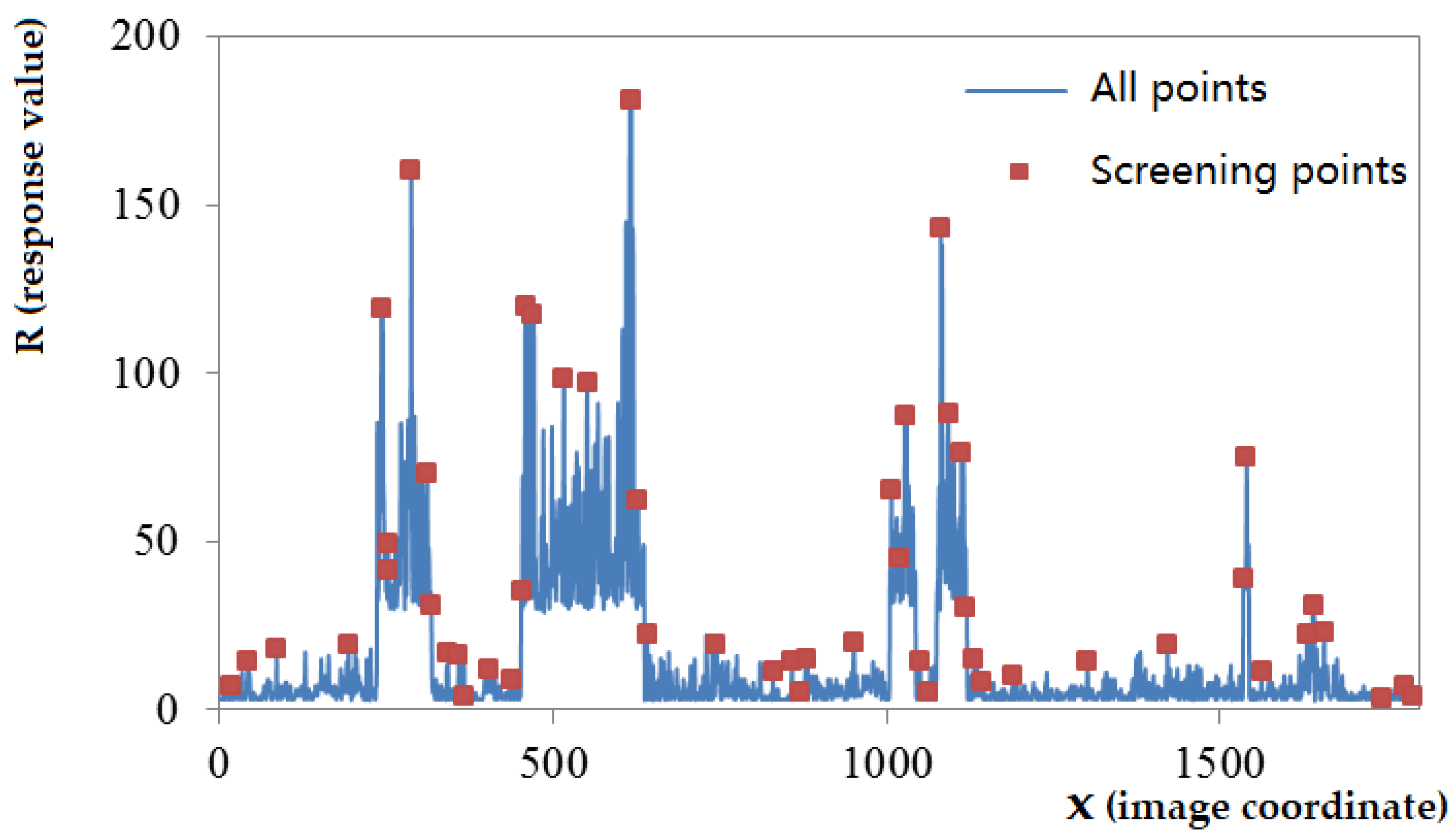
To propose a matching algorithm based on the weight of feature point response values by studying the homogenization of ORB features in visual odometry.
(2)
To incorporate a predictive motion model in keyframe pose estimation.

2. Visual Odometry

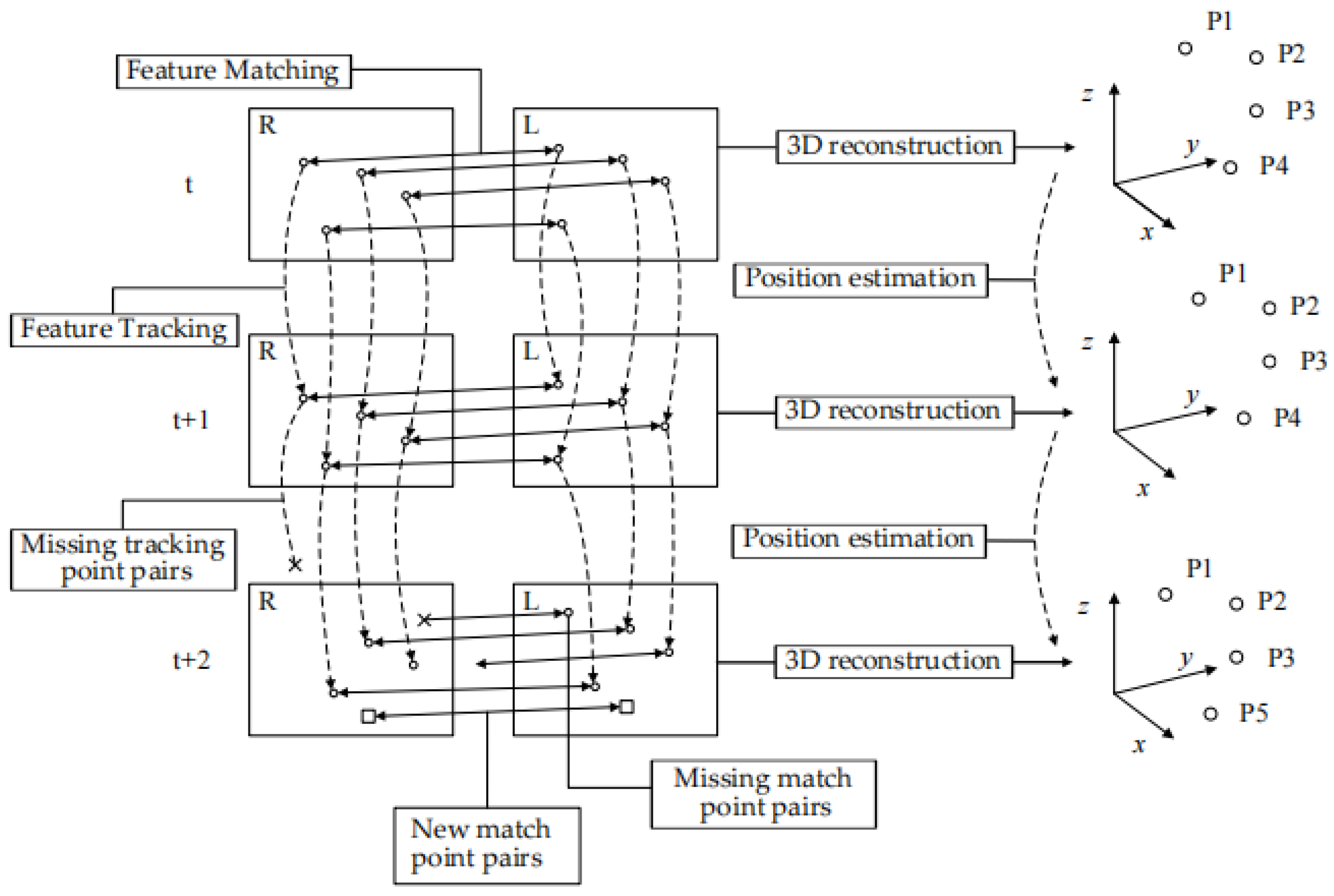
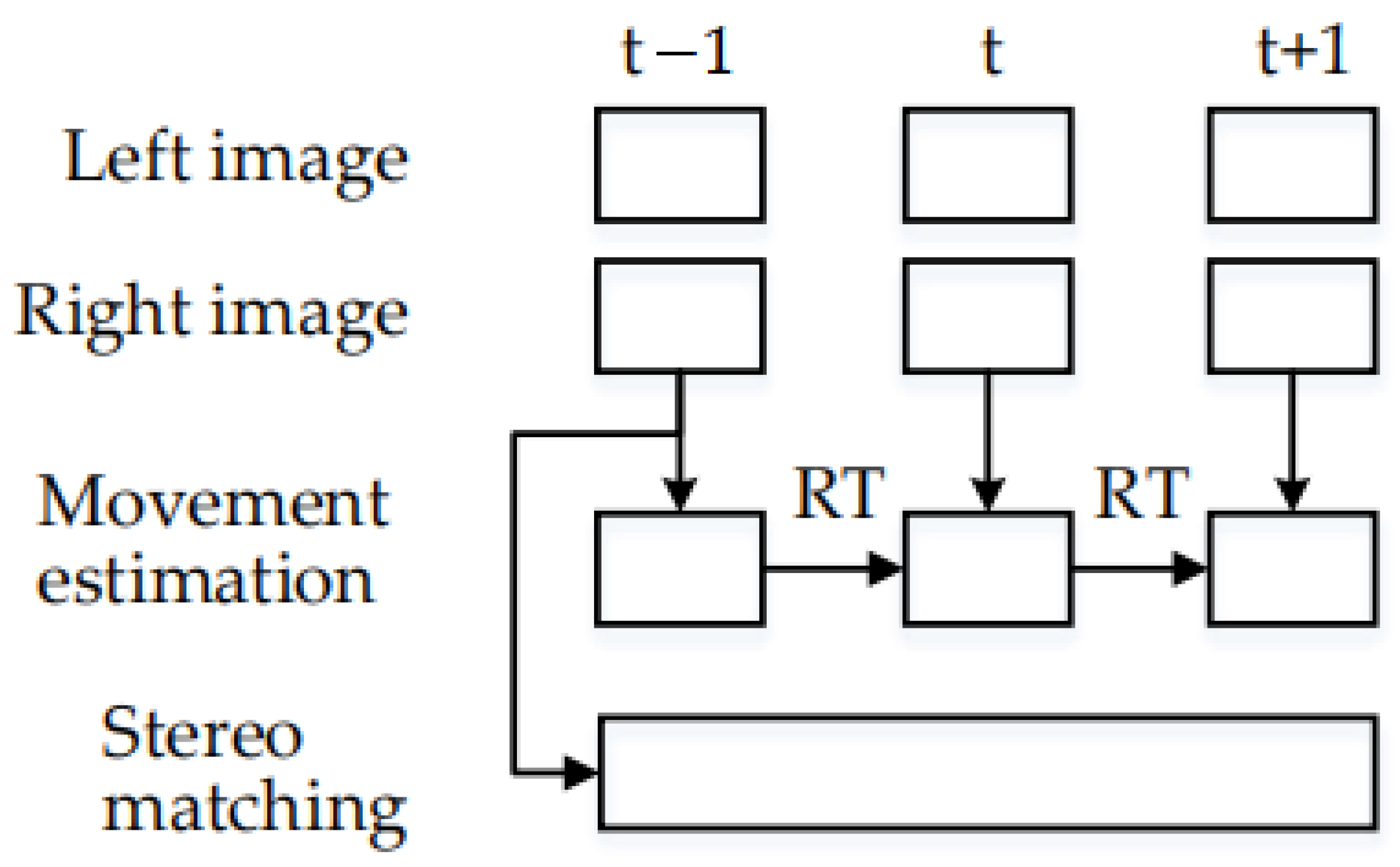
2.1. System Framework

A comprehensive stereo vision odometry system comprises four parts [17]: image acquisition and preprocessing, feature extraction and matching, feature tracking and 3D reconstruction, and motion estimation. The system flowchart is shown in Figure 1, and the specific process is as follows (R and L represent the left and right eyes, t and t + 1 represent different frames, and P represents the 3D position of the feature point):
(1)
Extracting feature points on the left- and right-eye images;
(2)
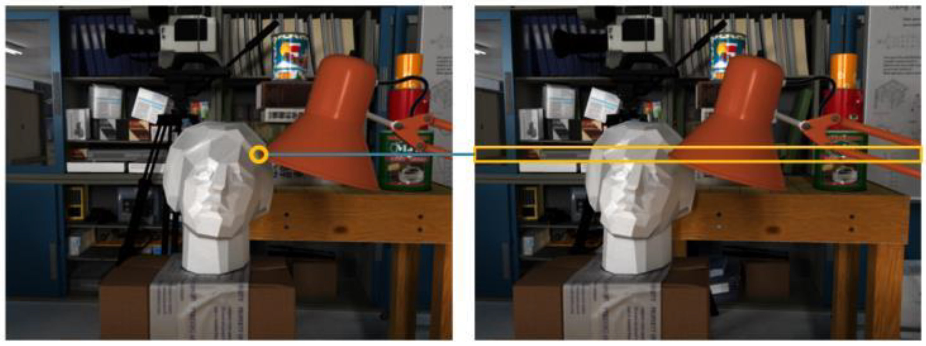
Matching feature points based on Euclidean distance and polar line constraints;
(3)
Reconstructing the 3D coordinates of matched feature point pairs;
(4)
Tracking feature points in the next frame of the image;
(5)
Calculating the camera pose by solving the minimum reprojection error problem for the feature points.
Figure 1. Block diagram of stereo vision odometer system.
Wevj 15 00123 g001

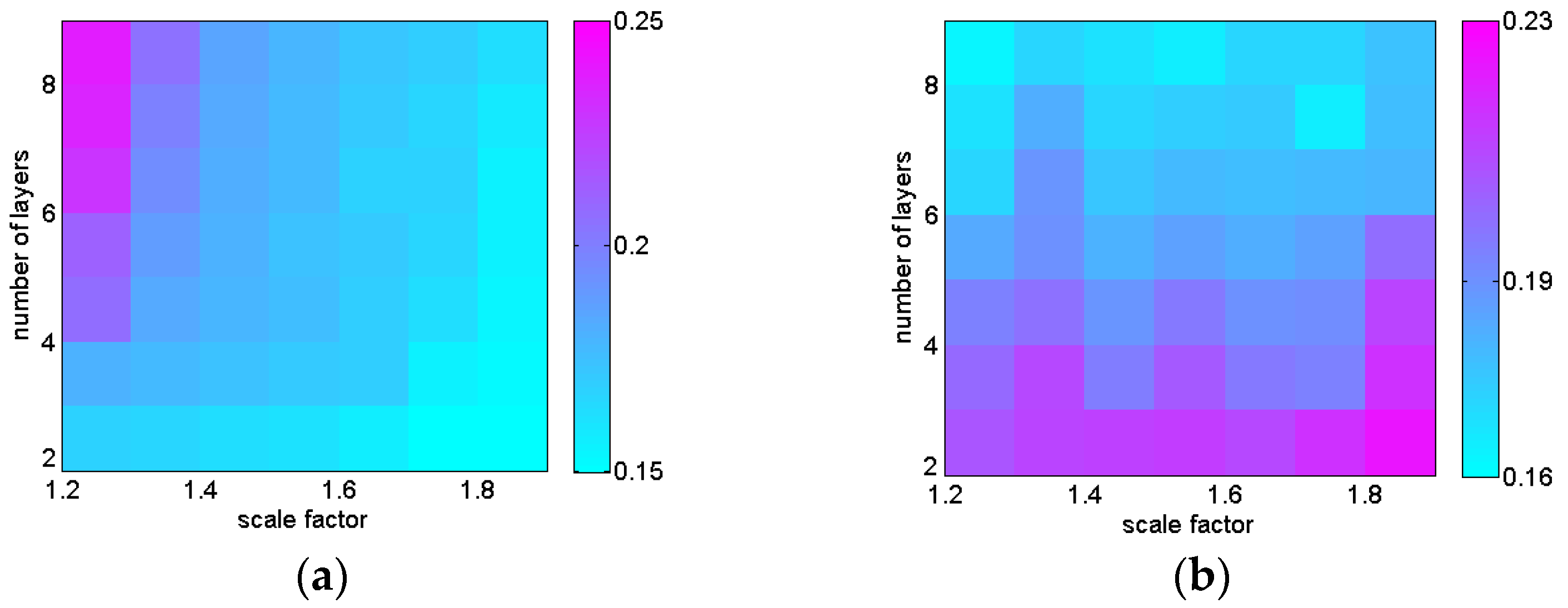
2.2. ORB Algorithm Parameter Selection

Selecting the appropriate scale parameter s and the number of pyramid layers N in OPENCV can reduce the computation time and the mismatch rate of ORB features during usage [18]. Assuming that the original image is at layer 0, the scale S i of layer i is
s i = s i
where s is the initial scale. Then, the image size of the layer i is
S i = ( H s i ) × ( W s i )
The original image is sized H × W . The scale parameter s of the above equation determines the size of each layer of the image in the pyramid. The larger the scale parameter, the smaller the image in each layer. In this paper, experiments were conducted on 05 sequences from the KITTI dataset, exploring various parameter combinations to select the most suitable configuration.
The comparative results of the parameters are shown in Figure 2. The vertical coordinates represent a change in the number of pyramid layers from 2 to 8. The horizontal coordinates represent variation in the scale parameter from 1.2 to 1.8. The color of each square in the figure then represents the size of the corresponding result. In Figure 2a, the total time from ORB feature extraction to matching is presented for different parameter combinations. The results indicate that as the number of pyramid levels increases, the computation time also increases, while an increase in the scale parameter leads to a reduction in computation time.
Figure 2b gives the mismatch rate when matching ORB feature points with different combinations of parameters. From the results, it can be seen that when the number of pyramid layers increases, the mismatch rate decreases significantly. Similarly, when the scale parameter becomes larger, the increase in the mismatch rate is smaller. Comprehensively considering the computational efficiency and matching accuracy, the scale parameter of the ORB feature is set to 1.8 and the number of layers in the image pyramid is 8.

3. Improvement of ORB Features

3.1. Calculation of Different Texture Area Weights

In the actual extraction process of ORB features, it is necessary to divide the image into several smaller regions for feature point extraction. Simultaneously, we must ensure that the number of feature points in each region remains consistent. The main steps are as follows [19]:
  • Segmentation of the image;
  • Extracting feature points;
  • Axing the extraction condition and extracting again if the number of feature points in the region is less than the minimum threshold.
If the number of features exceeds the upper threshold, then we select the Harris response values of the largest few and discard the others. (The basic principle of Harris corner detection is to slide a small window over the image and calculate the brightness changes in the window in various directions. When sliding the window over a corner, the corresponding brightness changes are typically large, regardless of the direction of the window. The Harris response is based on the magnitude and direction of these brightness changes to assess the salience of corners).
Figure 3a shows the sequence 05 from the KITTI dataset with a resolution of 1226 × 370. From the figure, it can be seen that without regional division, feature points are mainly concentrated at the contours of plants and houses. This situation results in similar descriptions between similar feature points, which can lead to mismatches, making their calculation results subject to large errors.
Firstly, the image is segmented to achieve a more uniform distribution of feature points throughout the image. For an image of original size W × H , given the segmentation coefficients s w and s w for width and height, the width and height of the image are divided equally as follows [20]:
n w = W s w , n h = W s h
The FAST parameter for the initial extraction of features in each region after segmentation is 30; if no feature points are extracted, the parameter is changed to 3 to extract them again. It can be seen from Figure 3b that the feature points extracted after region segmentation are more evenly distributed in the image. The next step is to filter the feature points in each region according to their Harris response values, and keep a few points with the largest response values in each region.
As the above screening process compares the response values of the feature points in each region, what is retained is only locally optimal. The relationship between the response values of the feature points before and after screening is given in Figure 4, where the blue curve indicates the response values of all 1862 feature points, and the red dots indicate the response values of the final feature points obtained after screening. As seen in the figure though, there are a considerable number of feature points that are extreme points of local response values. However, their response values are still low on the whole, which indicates that these points are not obvious for the corner points relative to the other points.
This point feature homogenization ensures that the feature points are distributed as uniformly as possible, but it also makes the corner point properties of some of the feature points very poor. This approach performs well in scenarios with abundant textures; however, in environments with insufficient texture richness, it may result in the suboptimal matching of feature points. In order to solve the above problems, the image regions are differentiated. For the image I ( x , y ) (which represents the grey value at point (x, y)), a matrix is computed [21]:
G = ( I x I y ) T ( I x I y )
The two eigenvalues of the matrix G represent the texture information of the region. When both eigenvalues are larger, it means that the region is a high-texture region; when the opposite is true, it means that the region is a low-texture region [22].
For regions of different textures, different weights are given. That is, the weights should be small for low-texture areas of the image, while for high-texture areas of the image, the weights should be large. The definition of weight w is as follows [23]:
w = min ( e i g e n v a l u e ( G ) )
The weight values are determined by the grayscale gradient of the pixel points in the local region of the image. This results in feature points with weights that are uniformly distributed over the image, ready for feature tracking and motion estimation.

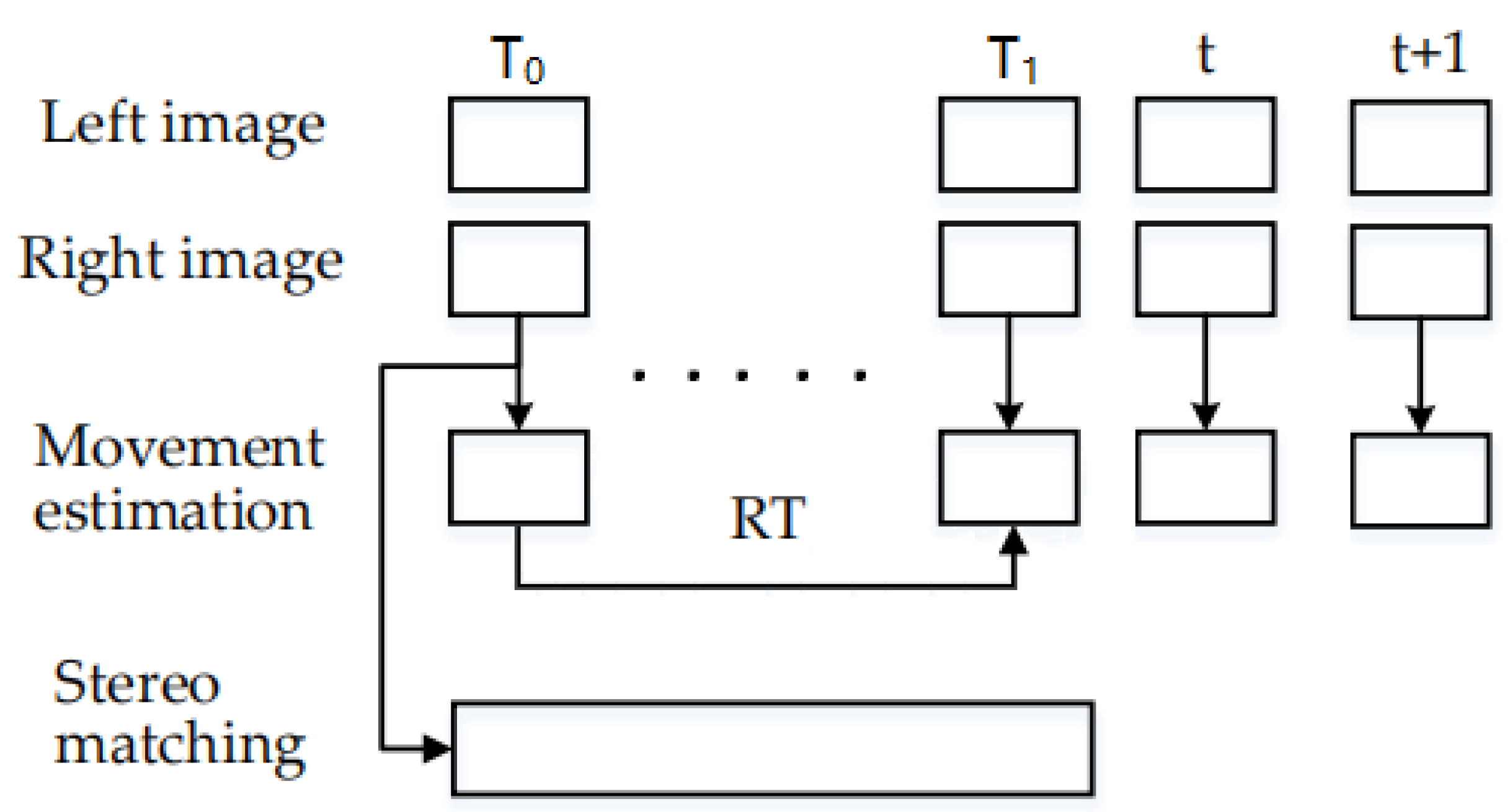
3.2. Keyframe-Based Predictive Motion Model

Next is a process for the stereo matching of feature points under successive frames, the aim of stereo matching is to find the corresponding projection points of the same spatial point in images acquired from different viewpoints [22]. For a parallel binocular vision system, polar constraints can be utilized for feature matching between left and right images. From the pairwise polar geometry, let the projection points of the same spatial point P on the left and right images be p 1 and p 2 ; then the corresponding point p 2 of the point p 1 must be on the polar line l 2 corresponding to p 1 . In this way, when searching for matching points, it is only necessary to search in the domain of the polar line. For example, in Figure 5, the yellow circle in the left figure indicates the feature point, and the yellow rectangular box in the right figure indicates the search range of feature matching.
For the feature matching problem of inter-frame images, the robustness and real-time performance of the visual odometry will not be guaranteed if we only rely on the unique constraints to reduce the error. Currently, the method of estimation using a motion model is used in front- and back-frame feature point matching to narrow down the search scope to solve the above problem [24]. According to the front- and back-frame images, to estimate the motion of the system, we calculate the position of the feature point in the image of moment t at moment t + 1 under this model and search for the best matching point around this position, as shown in Figure 6.
In the above method, the overlap between neighboring frames increases for slower vehicles. The projections of the feature points are basically unchanged; too much speed produces a large number of blurred frames and makes the feature points difficult to match. Too fast or too slow leads to high sensitivity of the system to errors. To solve this problem, we propose utilizing keyframes for motion model estimation, these keyframes are characterized by the easy identification of feature points between adjacent keyframes. The current frame is considered a key frame only if the mean Euclidean distance of all matching points between the current frame and the previous key frame falls within a certain threshold range.
d min < d k i , k i 1 < d max
  • d min —the minimum value of the distance threshold;
  • d max —the maximum value of the distance threshold;
  • d k i , k i 1 —the mean value of the Euclidean distance of the 3D coordinates of all matching points of the i th keyframe and the i 1 th keyframe.
The specific steps are as follows:
Set the first input frame as the reference frame (also the key frame), and calculate subsequent frames with this key frame until the frame that meets the threshold becomes the reference frame. Repeat this process to find all the key frames. As shown in Figure 7, T 0 represents the reference keyframe, T 1 represents the current keyframe, and R T represents the calculation in between. The motion obtained from the computation of the two keyframes is used to estimate the motion of the current frame and the next frame. This motion model is then used to compute the position of the feature point in the image at moment t for moment t + 1 , and loop around that position to obtain the early best match.

3.3. Three-Dimensional Reconstruction

The above improvements require recalculation of the 3D reconstruction process. The 3D reconstruction is first performed using the matched feature point pairs on the image. Then, the coordinates of the computed 3D points and the computed camera matrix are utilized for a second projection, called reprojection. Suppose that the P i space coordinate point is [ X i , Y i , Z i ] T and the p i pixel coordinate point is [ u i , v i ] T ; its Lie algebra projection formula is
d i p i = K exp ( ξ ) P i
where d i is the distance from point P i to the camera in three dimensions;
  • P i represents the 3D space coordinates;
  • K is the camera’s intrinsic parameter matrix;
  • p i represents the 2D spatial coordinates;
  • ξ is the R P i + t of the Lie group form; and R and t are the rotation and translation matrices of the camera in motion.
Errors are always inevitable due to the imperfect precision of the equipment, human factors, and the influence of external conditions. So, there is a certain projection error between the projection points; this error is called the reprojection error. In order to deal with the problem of error in these projection points, the number of observations is often greater than the number of observations necessary to determine the unknown quantity. This means that redundant observations are required. Redundant observations can also lead to contradictions between observations. Optimizing the model eliminates these contradictions and makes it possible to obtain the most reliable results as well as accuracy [25].
By constructing a least squares problem with the reprojection error of all points as a cost function, we obtain Equation (8) [26]:
ξ = arg min ξ i p i 1 d i K exp ( ξ ) p i 2
For the calculation of the minimized reprojection error, the texture weight values of the feature points are added:
ξ = arg min ξ i w p i 1 d i K exp ( ξ ) p i 2
Before calculating the least squares optimization problem, it is necessary to know the derivative of each error term with respect to the optimization variables, i.e., linearization:
e ( x + Δ x ) e ( x ) + J Δ x
When the pixel coordinate error e is two-dimensional and the camera pose x is six-dimensional, J is a 2 × 6 matrix (henceforth referred to as the Jacobi matrix). The transformation to the spatial point sitting under the camera coordinates is marked as P , taking out its first three dimensions:
P = ( exp ( ξ ) P ) 1 : 3 = [ X , Y , Z ] T
Then, the camera projection model is
d p = K P
Eliminating d yields
u = f x X Z + c x , v = f y Y Z + c y
Consider the derivative of the change in e with respect to the amount of perturbation:
e δ ξ = lim δ ξ 0 e ( δ ξ ξ ) δ ξ = e P P δ ξ
where denotes the left multiplicative perturbation on the Lie algebra. With the relationship between the variables obtained, it is deduced that
( exp ( ξ ) P ) P = ( exp ( ξ ) P ) = [ I P 0 T 0 T ]
By taking the first three dimensions in the definition of P and multiplying the two terms together, we obtain the 2 × 6 Jacobi matrix:
e δ ξ = [ f x Z 0 f x X Z 2 f x X Y Z 2 f x + f x X 2 Z 2 f x Y Z 0 f y Z f y Y Z 2 f y f y Y 2 Z 2 f y X Y Z 2 f y X Z ]
This Jacobi matrix describes the first-order variation in the reprojection error with respect to the Lie algebra of camera poses. For the derivative of e with respect to P at e spatial point,
e P = e P P P
Regarding the second item, by definition,
P = exp ( ξ ) = R P + t
Then,
e P = [ f x Z 0 f x Y Z 0 f y Z f y Y Z 2 ] R
So, the two derivative matrices of the observed camera equations with respect to the camera pose and feature points are obtained.

4. Experimental Verification

4.1. System Validation

The KITTI dataset is used for research in the field of autonomous driving [27]; the KITTI dataset uses the data obtained from GPS and inertial guidance system measurements as the reference path. This paper used the KITTI dataset for the experiments. The images were acquired at 10 Hz, the image resolution was 1241 × 376, and the camera parameters are shown in Table 1.
Because different key frame intervals are obtained for different distance thresholds, it is necessary to know and find the effects of different key frame intervals on the accuracy of the system. There are 1101 frames of binocular images in the image sequence of KITTI dataset 01. The statistics of different key frame rates are shown in Table 2. There are five sets of experiments. The higher the number of key frames, the smaller the interval between the adjacent key frames indicated. Table 3 shows sequence 05.
Figure 8 presents the statistical analysis of the average translation and rotation errors of the system under different keyframe rates in sequences 01 and 05 of the KITTI dataset. From the results, it can be seen that the average localization error and rotation error have the same trend. As the keyframe rate becomes larger, the error of the system first decreases, and then, increases. Based on the above results, the keyframe rate is chosen to be appropriate at 10–12%.

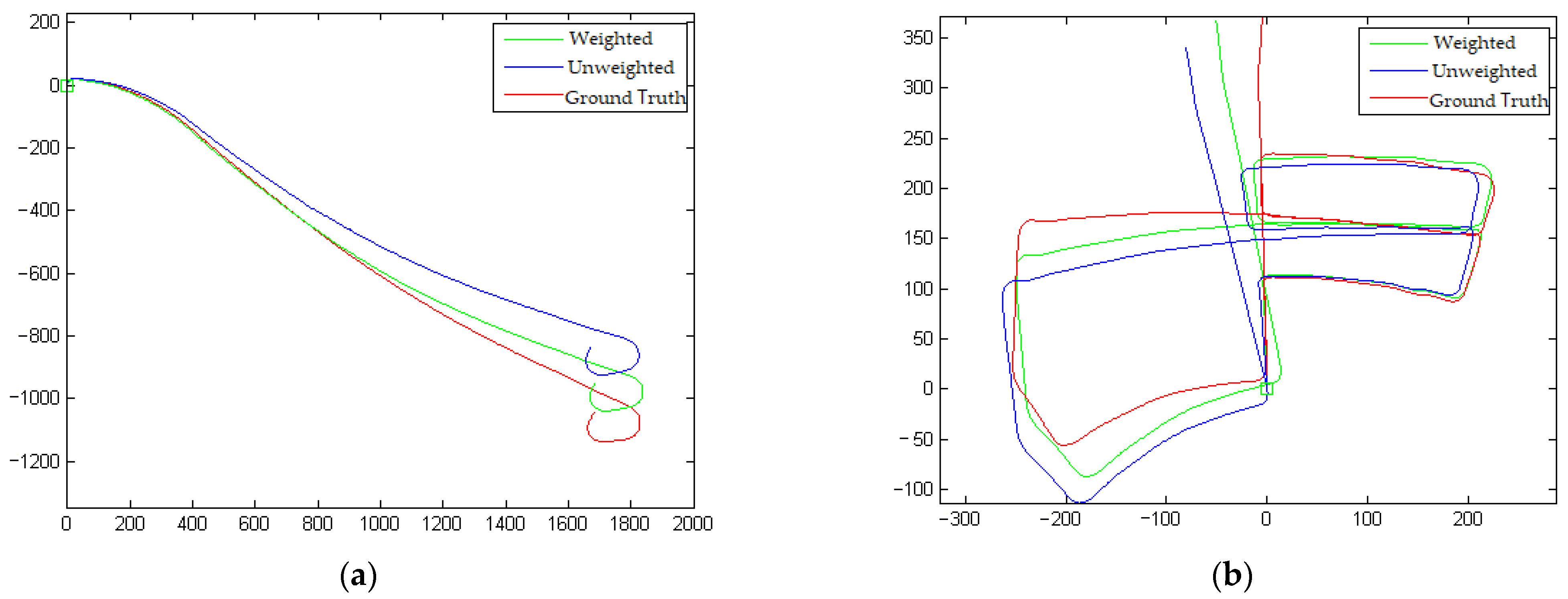
4.2. Verification of Texture Weighting Impact

Figure 9 shows the comparative computation results of image sequences 01 and 05 without weights and with weights. The coordinate units in the figure are in m. The environment of image sequence 01 is a highway and the environment of image sequence 05 is a small highway. The red path in the figure represents the groundtruth, the blue path is the calculation result when there is no weight, and the green path is the calculation result when there is weight. From the figure, it can be seen that the calculated results with weights are better than those without weights in both experiments. This initially verifies the effectiveness of the present method.

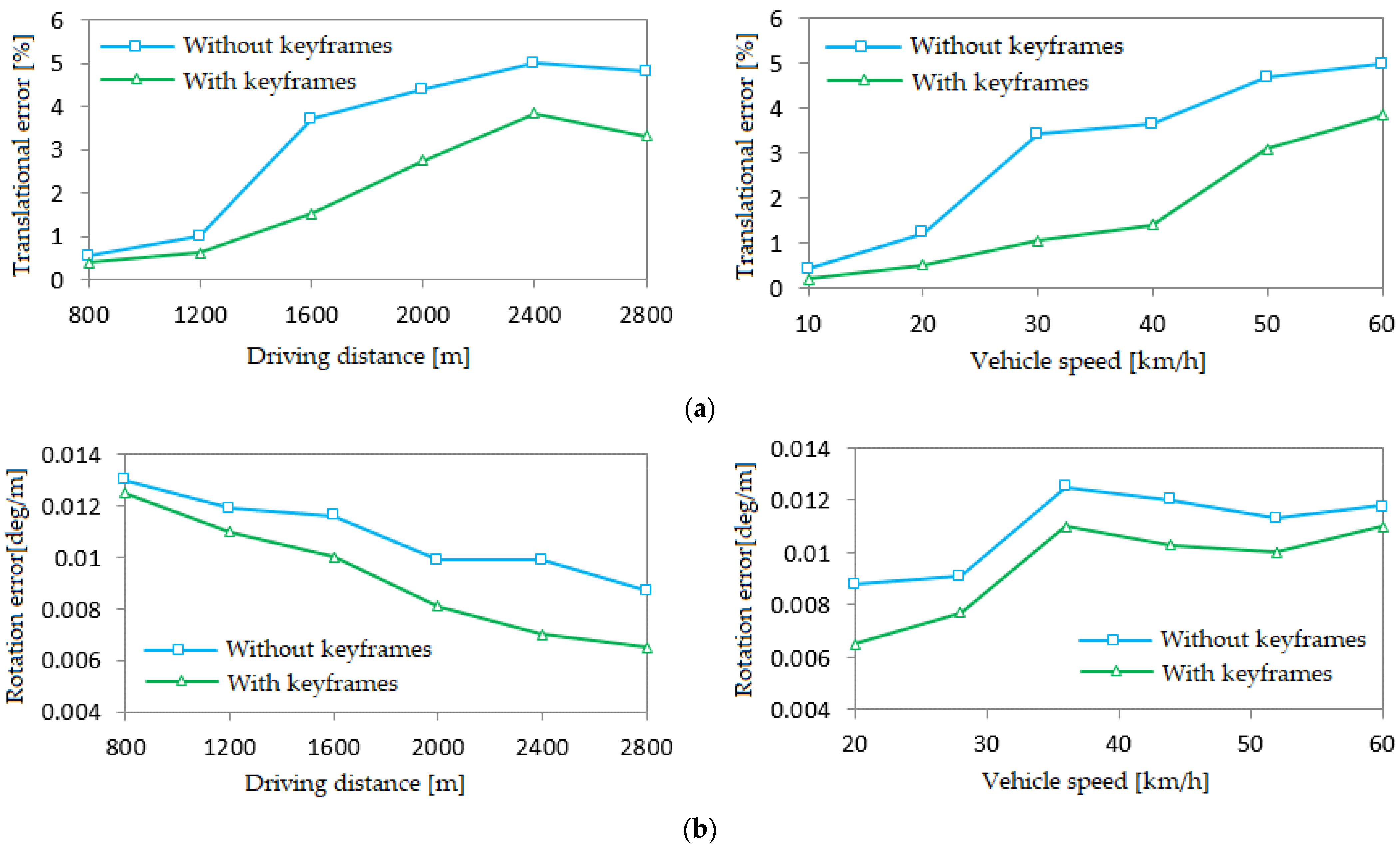
4.3. Verification of Keyframes

Figure 10 and Figure 11 give a comparison of the localization error and rotation error of image sequences 01 and 05, respectively. From the experimental results, the average translation error of image sequence 01 calculated with keyframes in Figure 10 is 2.8%, the maximum translation error is 3.8%, the average rotation error is 0.0095 deg/m, and the maximum rotation error is 0.0125 deg/m. The average translation error for image sequence 05 calculated with keyframes in Figure 11 is 2.2%, the maximum translation error is 2.9%, the average rotation error is 0.0087 deg/m, and the maximum rotation error is 0.0125 deg/m. The method of adding keyframes for inter-frame feature matching greatly reduces systematic error at low speeds.
In Table 4, the statistics of the time used by the visual odometer system for each main process in the calculation process are in in ms, Min represents the shortest time used, Max represents the longest time used, and Avg represents the average time used for each frame. The computer was configured with Intel dual core i7 2.4 GHz and 8G memory.
The translation and rotation errors of ORB-SLAM2 [28] and PL-SLAM [29] are compared using sequences 01 and 05 of the KITTI dataset, and the results are shown in Table 5. For sequence 01, both errors are smaller than in the other two algorithms. But for sequence 05, it is slightly worse than in the PL-SLAM algorithm and about the same as in ORB-SLAM2. This proves that the stability of this system is improved.

5. Conclusions

This paper focuses on the improvement of feature extraction and motion estimation in visual odometry, which obtains significant results.
  • The feature extraction part uses weight calculation for regions with different textures. High-texture regions have a greater matching weight, and low-texture regions have a smaller matching weight. So, the feature points can be evenly dispersed in the whole image.
  • In the part involving motion estimation, a predictive motion model of key frames is used. This makes the motion of feature points between neighboring keyframes obvious and improves efficiency. According to the test using the KITTI dataset, the key frame rate reaches 10–12% error minimization. Compared the translation and rotation errors with and without keyframes using the KITTI dataset, the translation and rotation errors are reduced.
  • A comparison is made with other open-source solutions. It is found that the visual odometer rotation error in this paper is significantly reduced from the other two rotation errors, but the translation error is not improved much. The stability of the system is improved considerably.

Author Contributions

Conceptualization, D.W. and Z.M.; methodology, W.X.; validation, D.W., Z.M. and W.X.; formal analysis, D.W.; investigation, Z.M.; resources, D.W.; data curation, D.W.; writing—original draft preparation, Z.M.; writing—review and editing, W.X.; visualization, Z.L.; supervision, H.H.; project administration, D.W.; funding acquisition, D.W. All authors have read and agreed to the published version of the manuscript.

Funding

This research were funded by Guizhou Forestry Science Research Program [2022] No. 26 and Guizhou Normal University Natural Science Research Program (Grants No. QSXM[2021]B18).

Data Availability Statement

The original contributions presented in the study are included in the article, further inquiries can be directed to the corresponding author.

Conflicts of Interest

The authors declare no conflict of interest.

References

  1. Li, S.; Wang, G.; Yu, H.; Wang, X. Engineering Project: The Method to Solve Practical Problems for the Monitoring and Control of Driver-Less Electric Transport Vehicles in the Underground Mines. World Electr. Veh. J. 2021, 12, 64. [Google Scholar] [CrossRef]
  2. Boersma, R.; Van Arem, B.; Rieck, F. Application of Driverless Electric Automated Shuttles for Public Transport in Villages: The Case of Appelscha. World Electr. Veh. J. 2018, 9, 15. [Google Scholar] [CrossRef]
  3. Latif, R.; Saddik, A. SLAM algorithms implementation in a UAV, based on a heterogeneous system: A survey. In Proceedings of the 2019 4th World Conference on Complex Systems (WCCS), Ouarzazate, Morocco, 22–25 April 2019; pp. 1–6. [Google Scholar] [CrossRef]
  4. Zhang, C.; Lei, L.; Ma, X.; Zhou, R.; Shi, Z.; Guo, Z. Map Construction Based on LiDAR Vision Inertial Multi-Sensor Fusion. World Electr. Veh. J. 2021, 12, 261. [Google Scholar] [CrossRef]
  5. Wu, D.; Ma, Z.; Xu, W.; He, H.; Li, Z. Research progress of monocular vision odometer for unmanned vehicles. J. Jilin Univ. Eng. Ed. 2020, 50, 765–775. [Google Scholar]
  6. Zeng, Q.H.; Luo, Y.X.; Sun, K.C. A review on the development of SLAM technology for vision and its fused inertia. J. Nanjing Univ. Aeronaut. Astronaut. 2022, 54, 1007–1020. [Google Scholar]
  7. Wu, D.; Ma, Z.; Xu, W.; He, H.; Li, Z. Methods and techniques for multi-motion visual odometry. J. Shandong Univ. Eng. Ed. 2021, 51, 1–10. [Google Scholar]
  8. Campos, C.; Elvira, R.; Rodriguez, J.J.G.; Montiel, J.M.M.; Tardos, J.D. ORB-SLAM3: An Accurate Open-Source Library for Visual, Visual-Inertial and Multi-Map SLAM. IEEE Trans. Robot. 2020, 37, 1874–1890. [Google Scholar] [CrossRef]
  9. Chen, Z.; Liu, L. Navigable Space Construction from Sparse Noisy Point Clouds. IEEE Robot. Autom. Lett. 2021, 6, 4720–4727. [Google Scholar] [CrossRef]
  10. Zhang, B.; Zhu, D. A Stereo SLAM System with Dense Mapping. IEEE Access 2021, 9, 151888–151896. [Google Scholar] [CrossRef]
  11. Seichter, D.; Köhler, M.; Lewandowski, B.; Wengefeld, T.; Gross, H.M. Efficient RGB-D Semantic Segmentation for Indoor Scene Analysis. In Proceedings of the 2021 IEEE International Conference on Robotics and Automation (ICRA), Xi’an, China, 30 May–5 June 2021; pp. 13525–13531. [Google Scholar]
  12. Mur-Artal, R.; Montiel, J.M.M.; Tardos, J.D. ORB-SLAM: A Versatile and Accurate Monocular SLAM System. IEEE Trans. Robot. 2015, 3, 1147–1163. [Google Scholar] [CrossRef]
  13. Bei, Q.; Liu, H.; Pei, Y.; Deng, L.; Gao, W. An Improved ORB Algorithm for Feature Extraction and Homogenization Algorithm. In Proceedings of the 2021 IEEE International Conference on Electronic Technology, Communication and Information (ICETCI), Changchun, China, 27–29 August 2021; pp. 591–597. [Google Scholar]
  14. Chen, J.S.; Yu, L.L.; Li, X.N. Loop detection based on uniform ORB. J. Jilin Univ. 2022, 1–9. [Google Scholar]
  15. Yao, J.; Zhang, P.; Wang, Y.; Luo, C.; Li, H. An algorithm for uniform distribution of ORB features based on improved quadtrees. Comput. Eng. Des. 2020, 41, 1629–1634. [Google Scholar]
  16. Zhao, C. Research on the Uniformity of SLAM Feature Points and the Construction Method of Semantic Map in Dynamic Environment. Master’s Dissertation, Xi’an University of Technology, Xi’an, China, 2022. [Google Scholar]
  17. Lai, L.; Yu, X.; Qian, X.; Ou, L. 3D Semantic Map Construction System Based on Visual SLAM and CNNs. In Proceedings of the IECON 2020 The 46th Annual Conference of the IEEE Industrial Electronics Society, Singapore, 18–21 October 2020; pp. 4727–4732. [Google Scholar]
  18. Ranftl, R.; Bochkovskiy, A.; Koltun, V. Vision Transformers for Dense Prediction. In Proceedings of the 2021 IEEE/CVF International Conference on Computer Vision (ICCV), Montreal, QC, Canada, 10–17 October 2021; pp. 12159–12168. [Google Scholar]
  19. Li, G.; Zeng, Y.; Huang, H.; Song, S.; Liu, B.; Liao, X. A Multi-Feature Fusion Slam System Attaching Semantic In-Variant to Points and Lines. Sensors 2021, 21, 1196. [Google Scholar] [CrossRef]
  20. Al-Mutib, K.N.; Mattar, E.A.; Alsulaiman, M.M.; Ramdane, H. Stereo vision SLAM based indoor autonomous mobile robot navigation. In Proceedings of the IEEE International Conference on Robotics and Biomimetics, Zhuhai, China, 6–9 December 2015; pp. 1584–1589. [Google Scholar]
  21. Fan, X.N.; Gu, Y.F.; Ni, J.J. Application of improved ORB algorithm in image matching. Comput. Mod. 2019, 282, 5–10. [Google Scholar]
  22. Xu, H.; Yang, C.; Li, Z. OD-SLAM: Real-Time Localization and Mapping in Dynamic Environment through Multi-Sensor Fusion. In Proceedings of the 2020 5th International Conference on Advanced Robotics and Mechatronics (ICARM), Shenzhen, China, 18–21 December 2020; pp. 172–177. [Google Scholar]
  23. Kitt, B.; Geiger, A.; Lategahn, H. Visual odometry based on stereo image sequences with RANSAC-based outlier rejection scheme. In Proceedings of the 2010 IEEE Intelligent Vehicles Symposium, La Jolla, CA, USA, 21–24 June 2010. [Google Scholar]
  24. Zhao, L.; Liu, Z.; Chen, J.; Cai, W.; Wang, W.; Zeng, L. A Compatible Framework for RGB-D SLAM in Dynamic Scenes. IEEE Access 2019, 7, 75604–75614. [Google Scholar] [CrossRef]
  25. Geiger, A.; Ziegler, J.; Stiller, C. StereoScan: Dense 3d reconstruction in real-time. IEEE Intell. Veh. Symp. 2011, 32, 963–968. [Google Scholar]
  26. Comport, A.I.; Malis, E.; Rives, P. Real-time Quadrifocal Visual Odometry. Int. J. Robot. Res. 2012, 29, 245–266. [Google Scholar] [CrossRef]
  27. Geiger, A.; Lenz, P.; Stiller, C.; Urtasun, R. Vision meets robotics: The KITTI dataset. Int. J. Robot. Res. 2013, 32, 1231–1237. [Google Scholar] [CrossRef]
  28. Mur-Artal, R.; Tardos, J.D. ORB-SLAM2: An Open-Source SLAM System for Monocular, Stereo, and RGB-D Cameras. IEEE Trans. Robot. 2017, 33, 1255–1262. [Google Scholar] [CrossRef]
  29. Gomez-Ojeda, R.; Moreno, F.; Scaramuzza, D.; Gonzalez-Jimenez, J. PL-SLAM: A Stereo SLAM System Through the Combination of Points and Line Segments. IEEE Trans. Robot. 2019, 35, 734–746. [Google Scholar] [CrossRef]
Figure 2. Calculation time and mismatch rate under different parameter matching. (a) Calculation time/10−2 s; (b) false match rate.
Wevj 15 00123 g002
Figure 3. Feature distribution. (a) Distribution of original features; (b) region segmentation results.
Wevj 15 00123 g003
Figure 4. ORB feature Harris response value.
Wevj 15 00123 g004
Figure 5. Extreme search.
Wevj 15 00123 g005
Figure 6. Motion model prediction.
Wevj 15 00123 g006
Figure 7. Motion model estimation based on keyframe.
Wevj 15 00123 g007
Figure 8. Comparison of errors at different key frame rates. (a) KITTI_01; (b) KITTI_05.
Wevj 15 00123 g008
Figure 9. Comparison of dataset results. (a) KITTI_01; (b) KITTI_05.
Wevj 15 00123 g009
Figure 10. Error contrast diagrams of sequence 01. (a) Translation error; (b) rotation error.
Wevj 15 00123 g010
Figure 11. Error contrast diagrams of sequence 05. (a) Translation error; (b) rotation error.
Wevj 15 00123 g011
Table 1. Binocular camera parameters.
Focal Length/mmCoordinates of Main PointAberration FactorBaseline/m
718.86(607.19, 185.22)0.000.54
Table 2. Key frame interval statistics of sequence 01.
Serial NumberNumber of FramesKey Frame CountKey Frame Rate (%)
11101665.99
21101888.00
3110111010.00
4110113312.05
5110116715.15
Table 3. Key frame interval statistics of sequence 05.
Serial NumberNumber of FramesKey Frame CountKey Frame Rate (%)
127612368.55
2276127710.03
3276131211.30
4276135812.97
5276141014.85
6276145616.52
7276149517.93
8276153419.34
Table 4. Algorithm calculation time statistics table.
Time (ms)MinMaxAvg
Feature extraction and matching14.634.620.7
3D reconstruction5.112.68.5
Movement estimation2.910.76.4
Total time23.952.335.6
Table 5. Comparison of different algorithms used on KITTI dataset.
KITTI
Dataset
ORB-SLAM2PL-SLAMOur
Translation Error (%)Rotation Error (deg/m)Translation Error (%)Rotation Error (deg/m)Translation
Error (%)
Rotation Error (deg/m)
012.750.01823.290.03012.740.0180
051.770.04501.670.01891.760.0451
Disclaimer/Publisher’s Note: The statements, opinions and data contained in all publications are solely those of the individual author(s) and contributor(s) and not of MDPI and/or the editor(s). MDPI and/or the editor(s) disclaim responsibility for any injury to people or property resulting from any ideas, methods, instructions or products referred to in the content.

