Article

Integrated Path Following and Lateral Stability Control of Distributed Drive Autonomous Unmanned Vehicle

1
Suzhou Automotive Research Institute, Tsinghua University, Suzhou 215200, China
2
Automotive Engineering Research Institute, Jiangsu University, 301 Xuefu Road, Zhenjiang 212013, China
*
Author to whom correspondence should be addressed.
World Electr. Veh. J. 2024, 15(3), 122; https://doi.org/10.3390/wevj15030122
Submission received: 30 January 2024 / Revised: 14 March 2024 / Accepted: 17 March 2024 / Published: 21 March 2024
(This article belongs to the Special Issue Intelligent Electric Vehicle Control, Testing and Evaluation)

Abstract

:
Intelligentization is the development trend of the future automobile industry. Intelligentization requires that the dynamic control of the vehicle can complete the trajectory tracking according to the trajectory output of the decision planning the driving state of the vehicle and ensure the driving safety and stability of the vehicle. However, trajectory limit planning and harsh road conditions caused by emergencies will increase the difficulty of trajectory tracking and stability control of unmanned vehicles. In view of the above problems, this paper studies the trajectory tracking and stability control of distributed drive unmanned vehicles. This paper applies a hierarchical control framework. Firstly, in the upper controller, an adaptive prediction time linear quadratic regulator (APT LQR) path following algorithm is proposed to acquire the desired front-wheel-steering angle considering the dynamic stability performance of the tires. The lateral stability of the DDAUV is determined based on the phase plane, and the sliding surface, in the improved sliding mode control (SMC), is further dynamically adjusted to obtain the desired additional yaw moment for coordinating the path following and lateral stability. Then, in the lower controller, considering the slip and the working load of four tires, a comprehensive cost function is established to reasonably distribute the driving torque of four in-wheel motors (IWMs) for producing the desired additional yaw moment. Finally, the proposed control algorithm is verified by the hardware-in-the-loop (HIL) experiment platform. The results show the path following and lateral stability can be coordinated effectively under different driving conditions.

1. Introduction

The autonomous unmanned vehicle (AUV) plays an essential role in an intelligent traffic system (ITS). It can liberate the driver’s control of the steering wheel and improve the safety and fluidity of the traffic system [1,2,3]. The distributed drive autonomous unmanned vehicle (DDAUV) is provided with four independent in-wheel motors (IWMs) to drive wheels, which makes the DDAUV have a drive redundancy [4,5].
Path following is an important research field of the DDAUV, which has been studied by many scholars. Considering the dynamic characteristics of tires, an autonomous front-wheel-steering system with the coupling control of displacement and force achieves good path following performance and road feeling through a robust control of the yaw rate [6]. In reference [7], sliding mode control (SMC) is utilized to deal with nonlinearities and uncertainties due to the complicated vehicle model, and an adaptive fuzzy SMC is employed to reduce the jitter to enhance the path following capability. Falcone et al. propose a control method using nonlinear model predictive control (NMPC) for path following [8], in which the current optimal front-wheel-steering angle can be obtained by status variables and control variables of the DDAUV combined with the prediction model [9]. But the complex nonlinear model and the process of rolling optimization will cause a heavy computational burden for the vehicle controller. The nonlinear vehicle model is linearized to improve computational efficiency [10]. However, in [11], many experiments show that this linear dynamics MPC method is suitable for path following at a low velocity. To solve this singularity at high velocity, a MPC method with switching following error is proposed [12], in which the controller can keep a small following error at a relatively high velocity. However, this control method fails to guarantee the lateral stability of DDAUV at this moment of switching. In addition, a linear quadratic regulator (LQR) with an adaptive Q matrix is used in [13,14] to overcome some of the shortcomings of the linear time-varying MPC (LTV-MPC) [15], which improves the computational efficiency of the algorithm, while the adaptive Q matrix is applied to effectively solve problems of disturbance generation. However, the proposed LQR controller does not have a predictive function to reduce the drastic motion of the steering wheels for a future moment, which may lead to a poor lateral stability [15,16]. Fitri Yakub demonstrates that the MPC controller has a prediction function for a future moment. The control of lateral stability and path following accuracy can be comparable to the LTV-MPC when a prediction module is introduced into the LQR controller [17]. In the above studies, scholars have paid more attention on steering maneuverability and path following accuracy. However, lateral stability is a critical factor in path following control, which should be investigated to guarantee driving safety.
For stability control, some scholars have studied vehicle stability by dealing with driving redundancy. References [18,19,20] apply a hierarchical architecture for stability control, where the upper controller solves for the additional yaw moment through the MPC, SMC or LQR method, and the lower controller is utilized to calculate the torque for IWMs under multiple constraints. Chen et al. design the status observers for estimating tire forces and vehicle velocity under different driving conditions [21]. The literature, in recent years, has started to investigate multiple actuators coupling and path following integrated control strategies to improve the lateral dynamic control. Reference [22] proposes a novel sliding mode control (SMC) method with Takagi–Sugeno (T-S) fuzzy rules. Xie et al. applies the LTV-MPC to obtain the steering angle. The weighting coefficient of following deviation on the sliding mode surface (SMS) is employed to obtain the additional yaw moment that can be produced through torque vector control. In reference [23], the SMC is used for coordinated control between path following and lateral stability, but the weight coefficient is not dynamically adjusted along with the change in the vehicle status. Reference [24] designs the objective function without considering the minimum slip of tires. Actuator failure is considered in references [10,25], so the path following model and torque allocation model are reconstructed. A monolithic control algorithm is utilized in reference [26] to achieve the purpose of integrated control based on the LTV-MPC method with the steering angle of steering wheels and torque of four IWMs as control variables.
Lateral control of the DDAUV is important for safe driving. The coordination control of path following and lateral stability should be emphasized due to the characteristics of vehicle nonlinearity and time-varying tire parameters.
In this paper, the coordinated control algorithm of path following and lateral stability for the DDAUV is proposed. The main contributions of this paper are given as follows:
(1)
The traditional LQR algorithm can solve the steady-state error problem of steering trajectory tracking by feedforward control, but it does not encompass roll optimization, and the control sequence within the control step can not be solved according to the predicted state deviation sequence, which makes the vehicle steering become radical. To solve this problem, this paper adds an adaptive prediction module based on LQR (Linear Quadratic Regulator) trajectory tracking control and judges the steering steady state according to the dynamic characteristics of the tire, so as to adjust the prediction time to make the steering more stable;
(2)
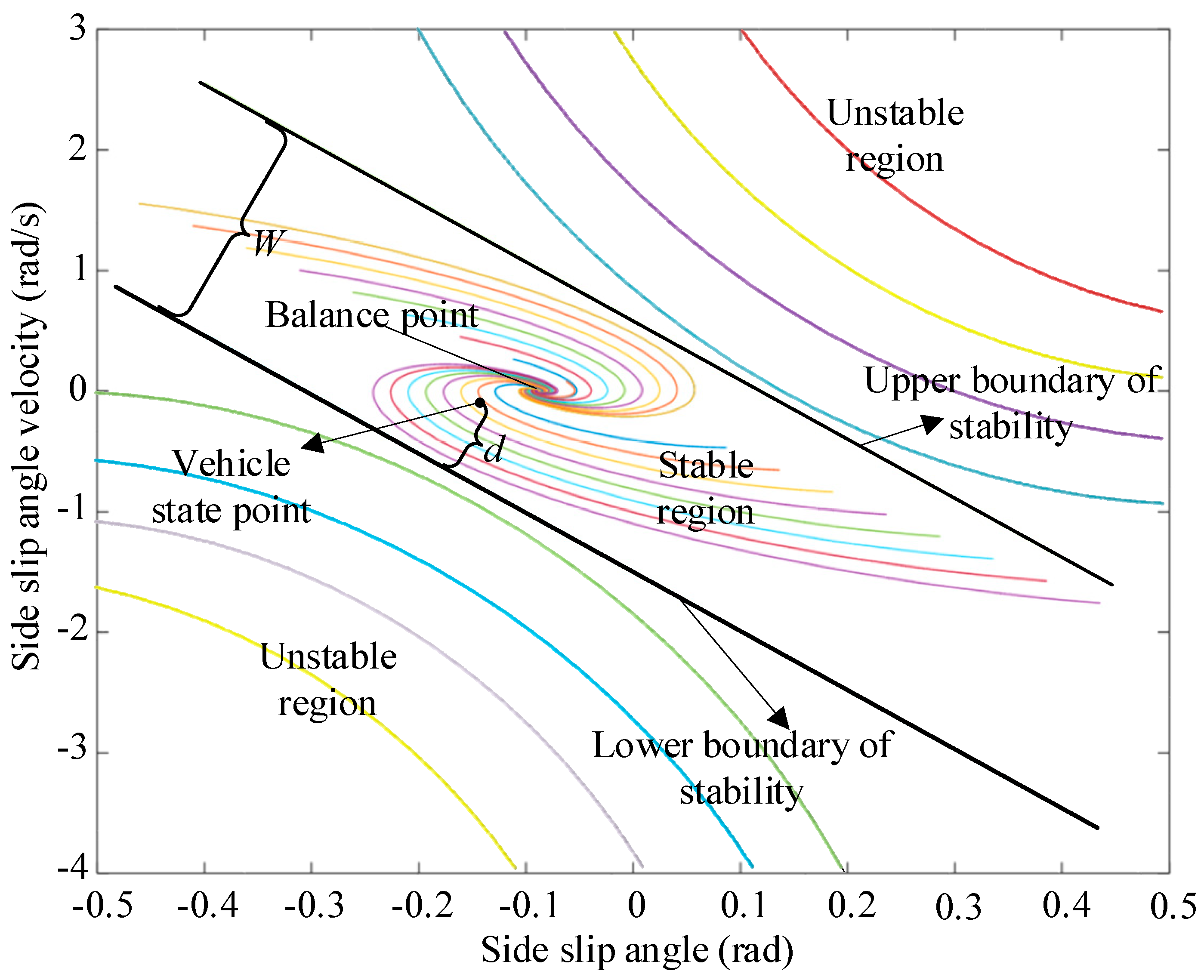
A stability compensation controller is designed by the additional yaw moment calculated by an improved SMC controller. The phase plane diagram of the sideslip angle and the sideslip angular velocity are used to judge the current stability state of the vehicle, so as to adaptively adjust the weight ratio of the sliding mode surface in the sliding mode control to coordinate the path following and lateral stability of the DDAUV;
(3)
Considering the slip and the working load of four tires, a comprehensive cost function is established and solved by the Karush–Kuhn–Tuckert (KKT) condition to allocate torque for IWMs. Moreover, the proposed algorithm is verified by the hardware-in-the-loop (HIL) experiments.
The rest of the paper is organized as follows: Section 2 introduces the framework of the proposed coordinated control algorithm and vehicle system model. Section 3 discusses the design of autonomous steering controller based on the APT LQR. Section 4 presents the design of stability compensation controller. In Section 5, HIL experiments are applied to verify the proposed coordinated control algorithm. Finally, a summary conclusion is given in Section 6.

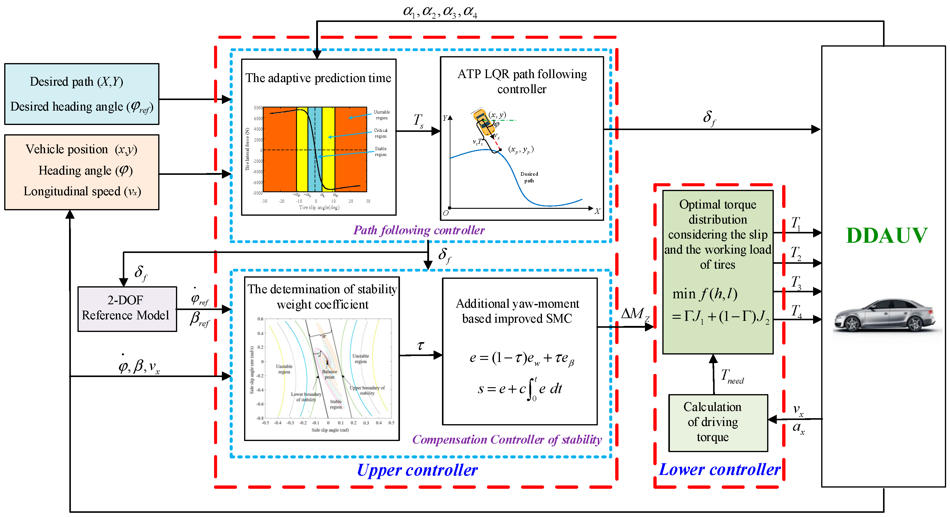
2. The Algorithm Framework and Model

2.1. Algorithm Framework

Figure 1 shows the hierarchical control architecture of the proposed coordinated control algorithm. The upper controller is composed of the APT LQR path following controller and lateral stability compensation controller. The lower controller is composed of a torque distribution controller and a calculation module of total driving torque. In APT LQR path following controller, the adaptive prediction time (APT) module based on tires dynamics adjusts the prediction time dynamically, and the APT LQR controller with prediction and feedforward functions is proposed to calculate the steering angle of autonomous front steering. In the stability compensation controller, the phase plane of side-slip angle is utilized to dynamically determine the stability of the DDAUV coefficient and adjust the weight coefficient of SMS. The improved SMC is employed to coordinate the additional yaw moment. According to the calculated total driving force and additional yaw moment, the torque distribution controller distributes the torque reasonably for four independent IWMs considering the minimum slip and working load of four tires, so that four wheels have enough stability margin to prevent the risk of extreme operation, which can develop a good closed-loop system. Furthermore, the 2-DOF vehicle model is used to calculate the reference yaw rate and reference side-slip angle. The calculation module of driving torque is applied to obtain the desired total driving torque to reach the target velocity for the DDAUV.

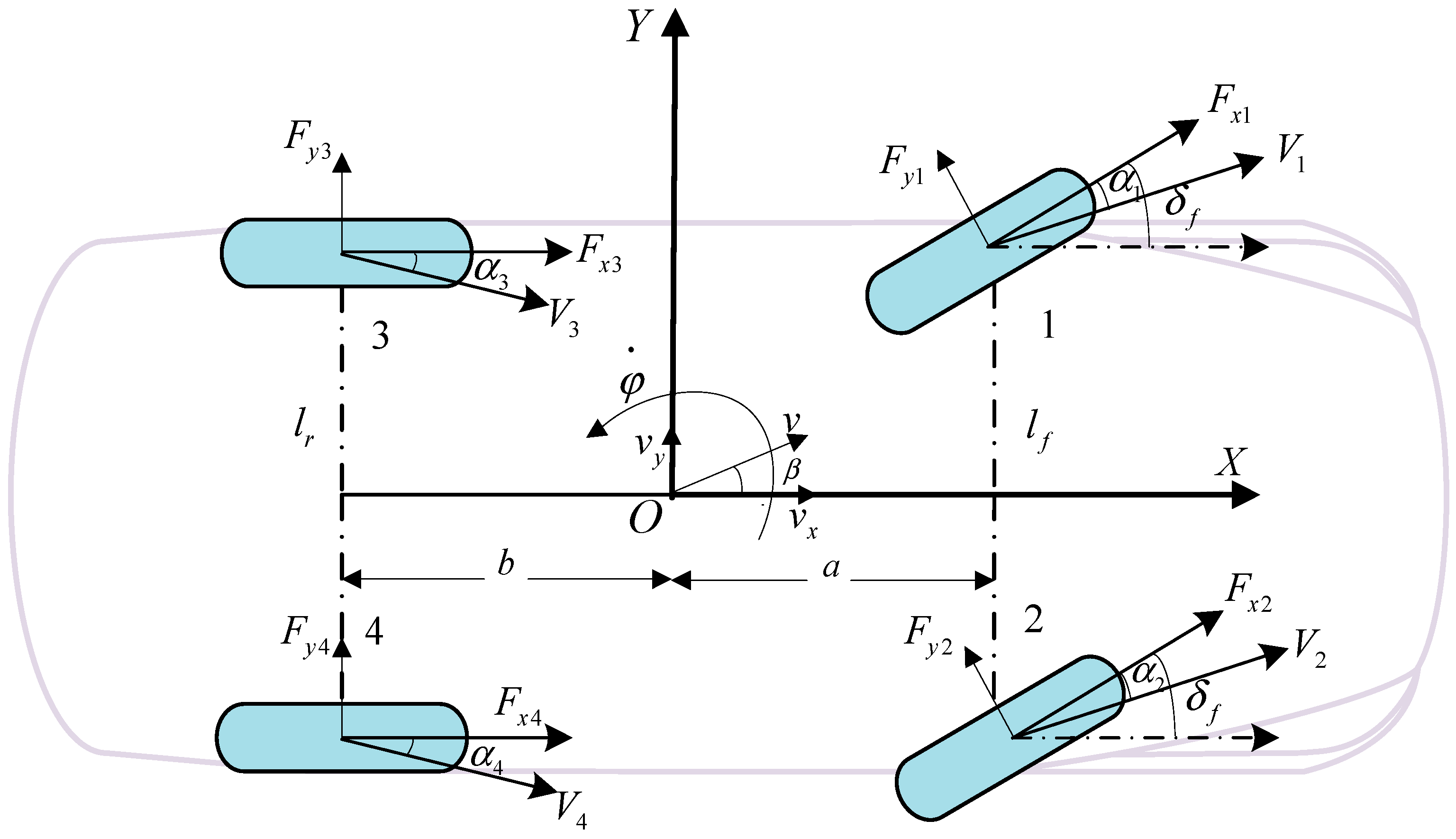
2.2. Vehicle Dynamic Model

A 2-degree-of-freedom (2-DOF) four-wheel vehicle model is utilized to describe the dynamic characteristics of the DDAUV in Figure 2. The basic parameters and variable symbols of the DDAUV are listed in Table 1.
The wheels are numbered 1, 2, 3 and 4, which represent the front left wheel, front right wheel, rear left wheel and rear right wheel, respectively. The lateral dynamic differential equation of the DDAUV is expressed [27]:
m ( v · y + φ · v x ) = ( F x 1 + F x 2 ) sin δ f + ( F y 1 + F y 2 ) cos δ f + F y 3 + F y 4 I z φ · · = a F y 1 + F y 2 cos δ f + l f 2 F y 1 F y 2 sin δ f b F y 3 + F y 4 + a ( F x 1 + F x 2 ) sin δ f + Δ M z
where m is equipment quality, vx is the longitudinal velocity, vy is the lateral velocity of the DDAUV, φ ˙ denotes yaw rate, and φ ¨ is the yaw angular acceleration.
Fxi (i = 1, 2, 3, 4) is the longitudinal force of the i-th wheel, Fyi (i = 1, 2, 3, 4) is the lateral force of the i-th wheel, δf denotes the steering angle of the front wheels, Iz is rotational inertia, a is the distance mass center to front wheels, b is the distance mass center to rear wheels, lf and lr are front wheel width and rear wheel width, respectively.
Δ M z = l f 2 F x 2 F x 1 cos δ f + l r 2 F x 4 F x 3
where ∆Mz is additional yaw moment. In the 2-DOF vehicle model, the lateral force could be regarded as a linear relationship with tire side-slip angle (Deng et al., 2021) [18].
F y i = C α i α i
where αi is tire side-slip angle of the i-th wheel, and Cαi is lateral tire stiffness of the i-th wheel. αi could be described as:
α 1 = α 2 = δ f + v y + a φ · v x α 3 = α 4 = v y b φ · v x
Considering that the front-wheel angle δf is relatively small, let sinδf = 0, cosδf = 1. Combining equations from Equation (1) to Equation (4), the lateral dynamic differential equation of the DDAUV model can be described as:
β · = ( a C α 1 + a C α 2 b C α 3 b C α 4 m v x 2 1 ) φ · C α 1 + C α 2 m v x δ f + C α 1 + C α 2 + C α 3 + C α 4 m v x β φ · · = ( a 2 ( C α 1 + C α 2 ) v x I z + b 2 ( C α 3 + C α 4 ) v x I z ) φ · a ( C α 1 + C α 2 ) I z δ f + a C α 1 + a C α 2 b C α 3 b C α 4 I z β + Δ M z I z

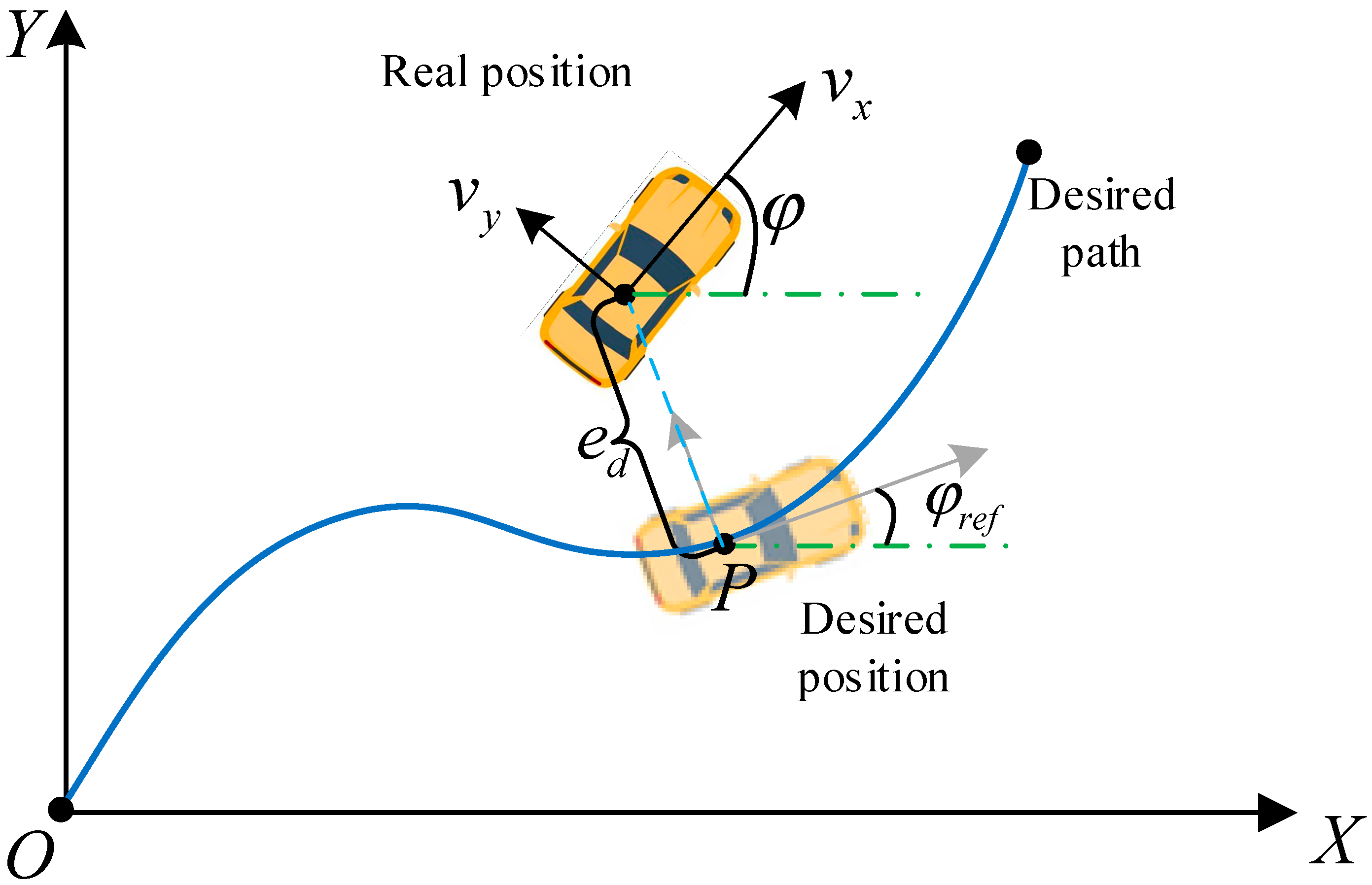
2.3. Path Following Model

The lateral deviation ed and heading deviation eφ can be employed to evaluate the path following performance when completing the unmanned task. The lateral deviation is defined as the deviation of the distance from the real position to the reference position. The heading deviation is the angle deviation from vehicle direction to tangential direction at the desire position [28,29]. As is shown in Figure 3. The reference position P means the closest point on the desired path from the center of vehicle.
When the vehicle is following the desired path, heading deviation can be expressed as [14]:
e φ = φ φ r e f
where φ is real heading angle of the DDAUV, and φref is reference heading angle.
From the geometric relationship shown in Figure 3, it can be found that the change rate of lateral deviation meets the following equation:
e · d = v x ( φ φ r e f ) + v y = v x e φ + v y
Therefore, the vehicle path following model can be described as:
e · · d = v x e · φ + v · y e · · φ = φ · · φ · · r e f

3. Design of Autonomous Steering Controller Based on the APT LQR

3.1. Design of LQR Path Following Controller

The linear quadratic regulator uses a linear feedback control law to form a closed-loop optimal control system, and its control object is a state space equation expressed in a linear form. In the trajectory tracking control, the state space equation required for LQR trajectory tracking control is constructed by using the dynamic differential equations of vehicle lateral and yaw degrees of freedom and the trajectory tracking model. In this paper, the position prediction module is added on the basis of LQR trajectory tracking, and the steering intensity is judged according to the dynamic characteristics of the tire, and the prediction time is adaptively adjusted to make the steering more stable.
In an autonomous steering controller, the additional yaw moment is unnecessary to be considered in the active steering control. ∆Mz is removed from Equation (1), and it can be transformed into:
v · y = C α 1 + C α 2 + C α 3 + C α 4 m v x v y + a ( C α 1 + C α 2 ) b ( C α 3 + C α 4 ) m v x v x φ · C α 1 + C α 2 m δ f φ · · = a ( C α 1 + C α 2 ) b ( C α 3 + C α 4 ) I z v x v y + a 2 ( C α 1 + C α 2 ) + b 2 ( C α 3 + C α 4 ) I z v x φ · a ( C α 1 + C α 2 ) I z δ f
Combining Equations (6)–(9), the path following model can be further expressed as:
e · · d = ( C α 1 + C α 2 + C α 3 + C α 4 m v x ) e · d ( C α 1 + C α 2 + C α 3 + C α 4 m ) e φ + a ( C α 1 + C α 2 ) b ( C α 3 + C α 4 ) m v x e · φ C α 1 + C α 2 m δ f + a ( C α 1 + C α 2 ) b ( C α 3 + C α 4 ) m v x v x φ · r e f e · · φ = a ( C α 1 + C α 2 ) b ( C α 3 + C α 4 ) I z v x e · d a ( C α 1 + C α 2 ) b ( C α 3 + C α 4 ) I z e φ + a 2 ( C α 1 + C α 2 ) + b 2 ( C α 3 + C α 4 ) I z v x e · φ a ( C α 1 + C α 2 ) I z δ f + a 2 ( C α 1 + C α 2 ) + b 2 ( C α 3 + C α 4 ) I z v x φ · r e f φ · · r e f
In general, the curvature of the road changes relatively smooth. In Equation (10), φ ˙ r e f can be ignored. Equation (10) can be rewritten as the form of state space:
X · = A l q X + B l q U + E l q G X = [ e d , e · d , e φ , e · φ ] T ;   U = [ δ f ] ;   G = [ φ · r e f ] A l q = 0 1 0 0 0 C α 1 + C α 2 + C α 3 + C α 4 m v x C α 1 + C α 2 + C α 3 + C α 4 m a ( C α 1 + C α 2 ) b ( C α 3 + C α 4 ) m v x 0 0 0 1 0 a ( C α 1 + C α 2 ) b ( C α 3 + C α 4 ) I z v x b ( C α 3 + C α 4 ) a ( C α 1 + C α 2 ) I z a 2 ( C α 1 + C α 2 ) + b 2 ( C α 3 + C α 4 ) I z v x B l q = 0 C α 1 + C α 2 m 0 a ( C α 1 + C α 2 ) I z ;   E l q = 0 a ( C α 1 + C α 2 ) b ( C α 3 + C α 4 ) m v x v x 0 a 2 ( C α 1 + C α 2 ) + b 2 ( C α 3 + C α 4 ) I z v x
To reduce the deviation in the state variables e d , e ˙ d , e φ , e ˙ φ , the LQR controller is used to make the state variables as small as possible by solving the current control variable U. Before solving that, as inspired by the literature [14], an objective function of the system is designed as:
J l q = 1 2 0 X T Q l q X + U T R l q U   d t
where Qlq represents the weight matrices for the state error, and Rlq represents the weight matrices for the control variable error in LQR status feedback control module. A large Qlq means that the system places more weight on the rapid attenuation of state deviation X, and a large Rlq means the system attaches more importance to the reduction in control variable U .
The optimal control variable can be expressed as:
U = K l q X = R l q 1 B l q T P X
where Klq = [K1, K2, K3, K4] is the coefficient matrix of the LQR status feedback control module. P is a constant matrix, which can be calculated by solving the Riccati equation [2].
To eliminate the steady-state error, the state feedforward control module is introduced. Therefore, the control variable can be calculated by:
U ˜ = δ f + δ q = K l q X + δ q
where δ f and δ q are calculated by feedback control module and feedforward control module. Equation (14) is substituted into Equation (11), so X ˙ = 0   X = 0 can be made when the system is stable. δ q can be expressed as:
δ q = φ · r e f v x m v 2 x a + b ( b C α 1 + C α 2 + a C α 3 + C α 4 ( K 3 1 ) ) a b + b K 3

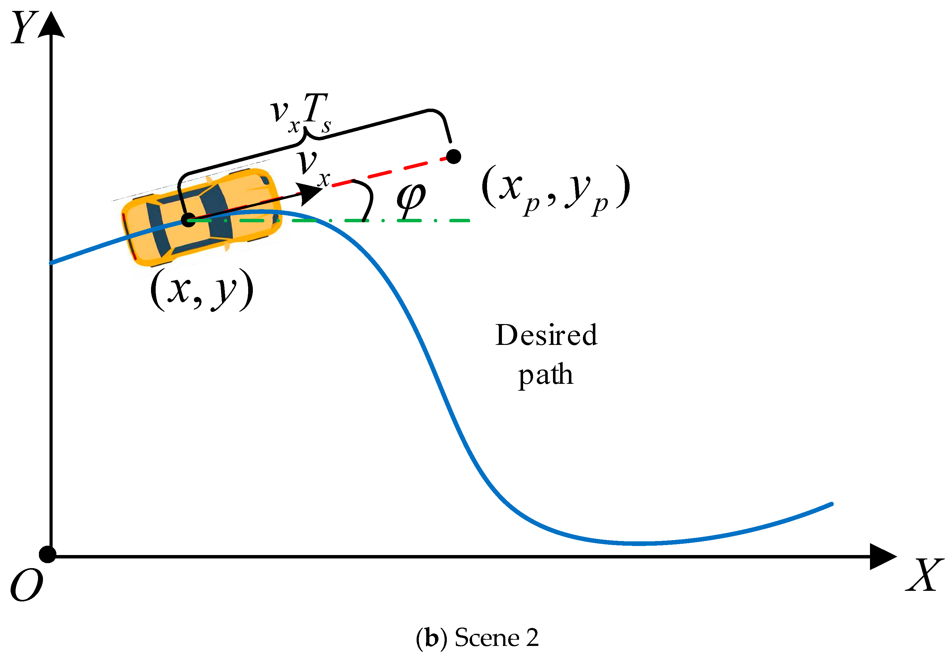
3.2. LQR Path Following Controller with Adaptive Prediction Time

Traditional LQR without a prediction module fails to reduce the over-drastic motion of the steering wheels according the road condition of the future period [21,30,31]. In Figure 4a, the lateral deviation and heading deviation are large, so the front steering wheel angle requires to be turned quickly to follow the path. However, the DDAUV is moving towards the correct path. Good path tracking and vehicle stability will be reached even not to adjust the steering angle. In Figure 4b, the lateral deviation and heading deviation of the DDAUV from the projection point are both small, but the vehicle needs to change the front wheel angle to adapt to the future path.
In this paper, APT LQR with adaptive prediction function is designed for path following, in which the prediction module is used to emulate the driving habits of humans by replacing the current vehicle position with the prediction position. That can be explained as follows.
When the prediction time is short, the deviation between the prediction position and the reference position is large, and the track tracking control pays more attention to the track tracking accuracy. However, when the prediction time is longer and the deviation between the predicted position and the reference position is small, the control is more focused on steering stationarity. Therefore, the prediction time should not be constant, but should be automatically adjusted according to the current stability state of the vehicle. When the stability state is good, the prediction time should be shorter to pay attention to the trajectory tracking accuracy, but when the stability state is poor, the prediction time should be longer to pay attention to the steering smoothness.
x p = x + v x T s cos φ y p = y + v x T s sin φ φ p = φ + φ · T s
where xp and yp are the information of the prediction position, φp is the predicted heading angle, and Ts means prediction time. Moreover, the velocity and yaw rate of the DDAUV are both considered constants when the prediction time is short enough.
Ts should be dynamically adjusted along with the state of the DDAUV. When the stability state is good, the short Ts is design to enhance the path following ability. But when the stability state is poor, Ts should be increased to ensure the lateral ability. References [24,26,32] proved that the stability state of the DDAUV and tire dynamic characteristics are closely related. The tire side-slip characteristic is shown in Figure 5. The blue area represents the stable region, yellow areas represent the critical region, and orange areas denote the instable region.
Therefore, the prediction time Ts can be dynamically adjusted according to following equations.
T s = t 1 + c s θ
θ = m a x θ i i = 1 , 2 , 3 , 4
θ i = 0 α i < α L α i α L α U α L α L < α i < α U   1 α i α U
where t1 is the based prediction time from tests and looking-up table, cs is a coefficient to limit the prediction time, θi denotes the instability coefficient of the i-th tire, θ can be seen as a function of θi, αU is the upper boundary of critical instability, and αL is the lower boundary of critical instability.

4. Design of Stability Compensation Controller for Autonomous Steering

4.1. Description of Stability Compensation Controller

Sliding mode control is a kind of variable structure control system. The control structure of the system can change according to the set rules according to the current state of the system. It has the advantages of a fast response speed and strong robustness. Therefore, SMC is widely used in the control field of complex systems such as nonlinearity and uncertainty. When the controlled system performs sliding mode control in any initial state, the control process includes two stages. One is the reaching mode, that is, under the action of the control law, where the system state error moves from the initial point to the designed sliding mode surface within a certain time. The second is the sliding mode, that is, the system state error slides along the sliding mode surface to the flat under the control law. However, due to the influence of system inertia, uncertain disturbance, and control lag, the chattering phenomenon will inevitably occur in the sliding process.
As the DDAUV is an overdrive redundant system, the four IWMs can generate the indicated torque independently [33,34]. A stability compensation controller is designed to improve lateral stability, then the minimum slip and working load of four tires are used as the control objectives to ensure that the vehicle can maintain a balance between maneuverability and lateral stability [35].
The yaw rate and side-slip angle of the DDAUV are applied to describe the lateral stability [26,36]. Therefore, the comprehensive error e can be designed as:
e = ( 1 τ ) e φ ˙ + τ e β
where e φ ˙ is error of the yaw rate, eβ is error of side-slip angle, and τ is stability weight coefficient.
As the linear SMS fails to guarantee that the initial state is located on the SMS [37], the integral term is introduced, and the SMS is shown as follows:
s = e + c 0 t e   d t = ( 1 τ ) ( φ · r e f φ · ) + τ ( β r e f β ) + c 0 t ( 1 τ ) ( φ · r e f φ · ) + τ ( β r e f β ) d t
where c is a positive constant. The large c means that it takes short time to reach the stability state. But the large c will cause severe jitter of the SMC. In this paper, c is designed as 0.6 through repeated tests.
The first order derivative of Equation (21) can be shown as:
s ˙ = ( 1 τ ) ( φ · · r e f φ · · ) + τ ( β ˙ r e f β ˙ ) + c ( 1 τ ) ( φ · r e f φ · ) + c τ ( β r e f β )
Choosing a suitable convergence law will improve the dynamic quality of the improved SMC, which can suppress jitter of the system. In this paper, the saturation function is used as the convergence law to suppress jitter further. φ ¨ in Equation (5) is substituted into Equation (22), and letting s ˙ = K v s a t ( s ) The control variable ∆Mz can be obtained as:
Δ M Z = I z φ · · r e f + ( 1 1 τ 1 ) I z ( β ˙ r e f β ˙ ) + c I z ( φ · r e f φ · ) + c ( 1 1 τ 1 ) I z ( β r e f β ) a 2 ( C α 1 + C α 2 ) v x + b 2 ( C α 3 + C α 4 ) v x φ · + a δ f ( C α 1 + C α 2 ) β ( a C α 1 + a C α 2 b C α 3 b C α 4 ) I z K v s a t ( s ) 1 τ
sat(s) is the saturation function, expressed as:
where s a t ( s ) = 1 s 0 < s s / s 0 s 0 s s 0 1 s < s 0 , and where s0 is the positive parameter of saturation boundary.

4.2. The Adaptive Adjustment of Stability Weight Coefficient

The stability weight coefficient τ needs to be adjusted dynamically according to the stability state of the DDAUV, and the phase plane is applied to analyze the lateral stability state [24,26]. When the stability of the DDAUV motion system is favorable, the small τ makes the torque distribution mainly focus on the path following. On the contrary, the large τ makes it mainly focus on lateral stability when the stability is weak. In the scene, with a velocity vx 60 km/h, a front-wheel angle δf 3 deg, and a road adhesion coefficient μ 0.5, the phase plane is plotted in Figure 6. In Figure 6, the balance point is the convergence point of the vehicle motion in the stability state. The stability boundary is the boundary line between the stable region and the unstable region. The stability boundary can be described by:
B 1 β · + β B 2 + e w
where β is the side-slip angle, β · is the side-slip angle rate, B1 and B2 are the parameters of stability boundary corresponding to the road adhesion coefficient μ, ew denotes system disturbance, which may be ignored to simplify the problem due to its small value, and the relationship between B1, B2 and μ can refer to reference [18].
The DDAUV in the stable region can converge to the balance point by its own regulation, but it should be stabilized by applying the additional yaw moment in the instable region. In Figure 6, the indicator d, which means the deviation from the state point of the DDAUV to the lower boundary of stability, is introduced to describe the stability state. A small d leads to poor stability, for which a large stability weight factor is required. A large d implies a strong self-regulation ability. Therefore, τ can be designed as a small value to enhance the ability of path following. However, τ needs to be designed no less than 0.3 to ensure the emergency capacity of the DDAUV. τ can be calculated by:
τ = 1 2 d W 0 < d < 0.35 W 0.3 0.35 W d < 0.65 W 1 2 ( W d ) W 0.65 W d < W 1 d 0 , d W
where W denotes the distance between two boundaries of stability, d > 0 indicates the state point above the lower boundary, and d < 0 indicates the state below the lower boundary.

4.3. Design of Torque Distribution Controller

The purpose of the torque distribution controller is to distribute total driving torque to produce the desired additional yaw moment.
T 1 + T 3 = T n e e d 2 + 2 Δ M z R l f + l r T 2 + T 4 = T n e e d 2 2 Δ M z R l f + l r
where R is the tire working radius, Ti (i = 1, 2, 3, 4) is the driving torque, and Tneed is the total driving torque needed to reach the target velocity, which can be obtained through the vehicle driving equation.
Torque distribution coefficients h and l are introduced to further distribute the torque of the front and rear wheels as shown in Equation (27).
T 1 = h ( T 1 + T 3 ) T 2 = l ( T 2 + T 4 ) T 3 = ( 1 h ) ( T 1 + T 3 ) T 4 = ( 1 l ) ( T 2 + T 4 )
where h is the distribution coefficient of left IWMs, l is the distribution coefficient of right IWMs. The comprehensive cost function includes the following two objectives.
The tire utilization adhesion coefficient means the proportion of tire force to maximum tire force provided by the road, which is used to describe the tire working load [32,38]. The tire utilization adhesion coefficient and the first objective function can be expressed as:
ζ i = F x i 2 + F y i 2 μ 2 F z i 2
J 1 = min i = 1 4 ζ i
The second objective function is designed to control driving torques and make the longitudinal slip and lateral slip have the minimum value. The second objective function can be described as:
J 2 = min i = 1 4 s x i · F x i 2 + α i · F y i 2
where sxi is slip ratio of the longitudinal direction.
Before integrating the two control objectives, it is necessary to normalize the slip power of loss to the range of [0, 1]. At the same time, the DDAUV are inevitably constrained by ground adhesion, motion characteristics, and motor working capacity. The problem of torque vector control can be described as the optimization involving h and l, and the comprehensive cost function with many constraints can be shown following:
min f ( h , l ) = Γ J 1 + ( 1 Γ ) J 2 s . t . T 1 + T 2 + T 3 + T 4 = T n e e d ( l f + l r ) 2 R ( T 1 + T 3 ) ( T 2 + T 4 ) = Δ M z F x i F x i max T i T i max
where Γ is weight coefficient. f is the cost function involving h and l. After testing by many simulations and HIL experiments, Γ = 0.4 is advisable, Fxi max is the longitudinal adhesion, and Ti max is the peak torque the IWM can provide. It is obvious that the problem is a convex nonlinear quadratic programming (QP) problem. Therefore, KKT method can be used to solve the equation [39].

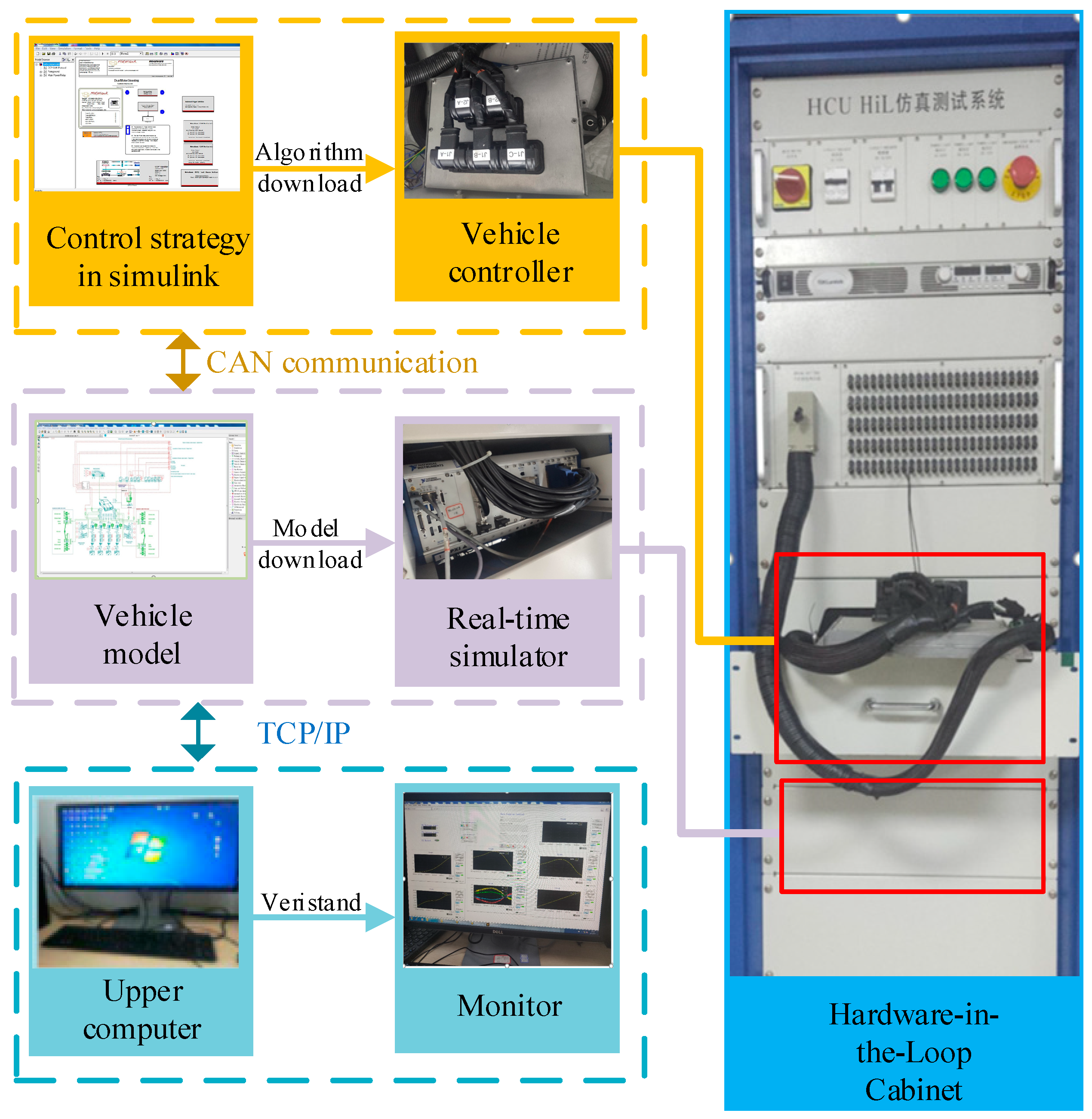
5. HIL Experiment Results and Analysis

The HIL experiment is carried out to test the effectiveness in a real controller as shown in Figure 7. The HIL experiment platform mainly consists of the main I/O module, the power supply module, the rapid prototyping controller, and the real-time simulator. The software mainly includes the lower software and the upper control strategy. The lower software includes communication protocols and diagnosis modules, etc. During the experiment, the DDAUV model in CarSim is compiled into dynamic chain file and downloaded to the real-time simulator. The proposed control strategy is compiled and downloaded to the real controller. The communication between the controller and real-time simulator is defined in NI Veristand software 2015.

5.1. DLC Manoeuvre on Low Adhesion Road

The experiment is set up to perform the double lane change (DLC) maneuver with the road adhesion coefficient μ = 0.5 and the velocity 60 km/h. Three different control strategies are designed for comparative analysis. “Compensation control” denotes that the compensation controller with adaptive stability weight coefficient is introduced into the APT LQR autonomous steering controller. “Autonomous steering” describes the APT LQR autonomous steering controller without the compensation controller. “Stability control” means the compensation controller with a fixed stability weight coefficient τ = 1. Figure 8 indicates the experiment results under DLC maneuver on a low adhesion road.
Figure 8a shows the path following of the DDAUV with three different control strategies. The path following accuracy in autonomous steering is more favorable than that in stability compensation control. And the path following accuracy with compensation control is more favorable than that in stability control. The path following accuracy is slightly decreased under compensation control than autonomous steering control, but the lateral stability can be significantly improved, which explains the possibility of stability compensation control while performing path following. Figure 8b shows the torque distribution coefficients in stability compensation control. The driving torque of four IWMs with the stability compensation is indicated in Figure 8c. The torque between left IWMs and right IWMs may be different to ensure stability when the DDAUV plans to change lane at high velocity, and even some IWMs generate reverse torque to reach the target additional yaw moment and improve wheels stability margins. In Figure 8d,e, the comparison results about the yaw rate and side-slip angle show that the stability of the DDAUV is improved widely under stability compensation control. The phase trajectory portrait for the three control strategies is shown in Figure 8f, where the phase trajectory deviates severely from the balance point under the autonomous steering control. However, the phase trajectory under the compensation control is around the balance point, which also explains that the stability compensation makes a favorable effect on the lateral stability and path following control.

5.2. DLC Maneuver on Joint Road

A joint road condition is utilized to further verify the maneuverability in the compensation control, wherein the joint road can be shown in Figure 9. When the DDAEV enters a low adhesion road from a high adhesion road, the ground cannot provide enough steering force for the steering wheels, which will lead to understeer. The proposed coordinated algorithm can help steering through differential tire forces as the following experiment results on joint road at the velocity 60 km/h under DLC maneuver, in Figure 10.
In Figure 10a, since stability control and compensation control both have auxiliary action, the steering behavior is significantly compensated. Figure 10b shows the torque distribution coefficients under the stability compensation control. Figure 10c indicates the torque fluctuation of four wheels under proposed coordinated algorithm. When the DDAUV passes through the road with an adhesion coefficient from 0.6 to 0.1 at about 1.2 s, the right IWMs are significantly strengthened to generate auxiliary steering yaw moment that can help avoid obstacles. Figure 10d,e show the yaw rate and side-slip angle. The yaw rate stops increasing when entering the joint part. That is because the low adhesion road fails to provide enough steering force. Although the stability control is more effective in a single adhesion road, the excessive additional yaw moment makes the side-slip angle increase rapidly when entering a low adhesion road. Stability control is unfavorable for the lateral stability instead in this scene, but the proposed compensation control method can effectively coordinate stability and maneuverability, which can also be confirmed through phase trajectory portrait Figure 10f. “Stability control” has a good performance in trajectory tracking, but compared with “Autonomous steering”, the side deflection angle of the center of mass is increased by about 18.1%. Therefore, the “Compensation control” method is more suitable for the coordinated control in this paper.

6. Conclusions

The integrated control of path following and lateral stability control is proposed to coordinate lateral stability and path following for the DDAUV. In the upper controller, the path following controller based on APT LQR method is designed, in which the position prediction module is designed and the prediction time is dynamically adjusted according to the tire dynamic characteristics. Based on the reference path, vehicle position, and status information, the APT LQR path following controller can calculate the appropriate front-wheel angle. The improved SMC is applied to seek the desired additional yaw moment. The SMS can be dynamically adjusted according to the lateral stability determined by the phase plane method to maintain a balance between lateral stability and path following. In the lower controller, considering the minimum slip and working load of four tires, a torque distribution algorithm is designed to allocate driving torque for producing the desired additional yaw moment. The results of HIL experiments show that the stability compensation controller plays a key role in coordination between the lateral stability and path following. The results show that the trajectory tracking and lateral stability of the hierarchical control architecture with the adaptive prediction module are well coordinated in different working conditions. The limitation of this paper is that it does not consider the influence of driving torque on the analysis of tire slip loss energy and the influence of vehicle speed change on vehicle trajectory tracking and lateral stability. Future research will be carried out from the following aspects.
(1)
Considering the great influence of driving torque on the loss energy from tire slip and the working efficiency of IWMs, future research will focus on the integrated control of stability and energy saving through torque vectoring control;
(2)
In this paper, the fixed speed condition is used in the HIL test, but the speed of the unmanned vehicle changes in the trajectory planned by the decision planning layer, and the speed has a certain influence on the vehicle trajectory tracking and lateral stability. Therefore, the influence of time-varying vehicle speed on its control performance should be considered when designing control strategies in the future.

Author Contributions

Conceptualization, Y.L. and Q.C.; methodology, Q.C.; software, J.A., Q.C. and Y.L.; validation, Q.C.; investigation, Y.L. and Q.C.; data curation, Q.C.; writing—original draft preparation, Q.C.; writing—review and editing, J.A., F.Z. and Y.L.; supervision, Y.L.; project administration, F.Z. and Y.L.; funding acquisition, Y.L. All authors have read and agreed to the published version of the manuscript.

Funding

This work is supported by National Natural Science Foundation of China (Grant No. 51705213), supported by State Key Laboratory of Intelligent Green Vehicle and Mobility (Grant No. KFY2409), supported by the Opening Project of Automotive New Technique of Anhui Province Engineering Technology Research Center (Grant No. QCKJ202201A), supported by the Opening Project of National Engineering Laboratory of Energy-saving Motor & Control Technique of Anhui University (Grant No. KFKT202215).

Data Availability Statement

The raw data supporting the conclusions of this article will be made available by the authors on request.

Conflicts of Interest

The authors declare no conflicts of interest.

References

  1. Chen, T.; Chen, L.; Xu, X.; Cai, Y.; Jiang, H.; Sun, X. Passive fault-tolerant path following control of autonomous distributed drive electric vehicle considering steering system fault. Mech. Syst. Signal Process. 2019, 123, 298–315. [Google Scholar] [CrossRef]
  2. Zhao, B.; Xu, N.; Chen, H.; Guo, K.; Huang, Y. Stability control of electric vehicles with in-wheel motors by considering tire slip energy. Mech. Syst. Signal Process. 2019, 118, 340–359. [Google Scholar] [CrossRef]
  3. Yao, X.; Gu, X.; Jiang, P. Coordination control of active front steering and direct yaw moment control based on stability judgment for AVs stability enhancement. Proc. IMechE Part D J. Automob. Eng. 2021, 236, 59–74. [Google Scholar] [CrossRef]
  4. Li, C.; Jiang, H.; Wang, C.; Ma, S. Estimation method of vehicle position and attitude based on sensor information fusion. J. Jiangsu Univ. (Nat. Sci. Ed.) 2022, 43, 636–644. [Google Scholar]
  5. Li, S.; Feng, Q. Control strategy of adaptive cruise system for electric vehicle driven by hub motor. J. Jiangsu Univ. (Nat. Sci. Ed.) 2023, 44, 125–132. [Google Scholar]
  6. Zhao, W.; Zhang, H.; Li, Y. Displacement and force coupling control design for automotive active front steering system. Mech. Syst. Signal Process. 2018, 106, 76–93. [Google Scholar] [CrossRef]
  7. Liu, C.; Sun, W.; Zhang, J. Adaptive sliding mode control for 4-wheel SBW system with ackerman geometry. ISA Trans. 2020, 96, 103–115. [Google Scholar] [CrossRef]
  8. Falcone, P.; Eric, H.; Borrelli, F.; Asgari, J.; Hrovat, D. MPC-based yaw and lateral stabilization via active front ste ering and braking. Veh. Syst. Dyn. 2008, 46, 611–628. [Google Scholar] [CrossRef]
  9. Li, Z.; Wang, P.; Liu, H.; Hu, Y.; Chen, H. Coordinated longitudinal and lateral vehicle stability control based on the combined-slip tire model in the MPC framework. Veh. Syst. Dyn. 2021, 161, 107947. [Google Scholar]
  10. Li, B.; Du, H.; Li, W. Fault-tolerant control of electric vehicles with in-wheel motors using actuator-grouping sliding mode controllers. Mech. Syst. Signal Process. 2016, 72, 462–485. [Google Scholar] [CrossRef]
  11. Chen, Y.; Li, Z.; Kong, H.; Ke, F. Model predictive tracking control of nonholonomic mobile robots with coupled input constraints and unknown dynamics. IEEE Trans. Ind. Inform. 2018, 15, 3196–3205. [Google Scholar] [CrossRef]
  12. Sun, C.; Zhang, X.; Zhou, Q.; Tian, Y. A model predictive controller with switched tracking error for autonomous vehicle path tracking. IEEE Access 2019, 7, 53103–53114. [Google Scholar] [CrossRef]
  13. Hu, C.; Wang, R.; Yan, F.; Chen, N. Output constraint control on path following of four-wheel independently actuated autonomous ground vehicles. IEEE Trans. Veh. Technol. 2015, 65, 4033–4043. [Google Scholar] [CrossRef]
  14. Lee, K.; Jeon, S.; Kim, H.; Kum, D. Optimal path tracking control of autonomous vehicle: Adaptive full-state linear quadratic gaussian (LQG) control. IEEE Access 2019, 7, 109120–109133. [Google Scholar] [CrossRef]
  15. Tavan, N.; Tavan, M.; Hosseini, R. An optimal integrated longitudinal and lateral dynamic controller development for vehicle path tracking. Lat. Am. J. Solids Struct. 2015, 12, 1006–1023. [Google Scholar] [CrossRef]
  16. Vivek, K.; Sheta, M.; Gumtapure, V. A comparative study of Stanley, LQR and MPC controllers for path tracking application. IEEE Int. Conf. Intell. Syst. Green Technol. (ICISGT) 2019, 13, 667–674. [Google Scholar]
  17. Yakub, F.; Yakub, Y. Comparative study of autonomous path-following vehicle control via model predictive control and linear quadratic control. Proc. Inst. Mech. Eng. 2015, 229, 1695–1714. [Google Scholar] [CrossRef]
  18. Deng, H.; Zhao, Y.; Feng, S.; Wang, Q.; Zhang, C.; Lin, F. Torque vectoring algorithm based on mechanical elastic electric wheels with consideration of the stability and economy. Energy 2021, 219, 119643. [Google Scholar] [CrossRef]
  19. Ardashir, M.; Hamid, T. A novel adaptive control approach for path tracking control of autonomous vehicles subject to uncertain dynamics. Proc IMechE Part D J. Automob. Eng. 2020, 234, 2115–2126. [Google Scholar]
  20. Guo, J.; Luo, Y.; Li, K. An adaptive hierarchical trajectory following control approach of autonomous four-wheel independent drive electric vehicles. IEEE Trans. Intell. Transp. Syst. 2017, 19, 2482–2492. [Google Scholar] [CrossRef]
  21. Chen, T.; Xu, X.; Chen, L.; Jiang, H.; Cai, Y.; Li, Y. Estimation of longitudinal force, lateral vehicle speed and yaw rate for four-wheel independent driven electric vehicles. Mech. Syst. Signal Process. 2018, 101, 377–388. [Google Scholar] [CrossRef]
  22. Ma, X.; Wong, P.; Zhao, J.; Xie, Z. Cornering stability control for vehicles with active front steering system using TS fuzzy based sliding mode control strategy. Mech. Syst. Signal Process. 2019, 125, 347–364. [Google Scholar] [CrossRef]
  23. Xie, J.; Xu, X.; Wang, F.; Tang, Z.; Chen, L. Coordinated control based on path following of distributed drive autonomous electric vehicles with yaw-moment control. Control Eng. Pract. 2021, 106, 104659. [Google Scholar] [CrossRef]
  24. Ren, B.; Chen, H.; Zhao, H.; Yuan, L. MPC-based yaw stability control in in-wheel-motored EV via active front steering and motor torque distribution. Mechatronics 2016, 38, 103–114. [Google Scholar] [CrossRef]
  25. Wang, H.; Cui, W.; Shu, L.; Tan, D. Stability control of in-wheel motor drive vehicle with motor fault. Part D J. Automob. Eng. 2018, 233, 3147–3164. [Google Scholar] [CrossRef]
  26. Park, G.; Han, K.; Nam, K.; Kim, H.; Choi, S. Torque vectoring algorithm of electronic-four-wheel drive vehicles for enhancement of cornering performance. IEEE Trans. Veh. Technol. 2020, 69, 3668–3679. [Google Scholar] [CrossRef]
  27. Feng, J.; Zhang, P.; Wang, W.; Qi, Q.; Song, B. Direct yaw moment control and realization mode of handling stability for high-clearance sprayer. J. Jiangsu Univ. (Nat. Sci. Ed.) 2022, 43, 657–665. [Google Scholar]
  28. Han, Z.; Xu, N.; Chen, H.; Huang, Y.; Zhao, B. Energy-efficient control of electric vehicles based on linear quadratic regulator and phase plane analysis. Appl. Energy 2018, 213, 639–657. [Google Scholar] [CrossRef]
  29. Li, S.; Sun, X. Active obstacle avoidance path planning based on improved artificial potential field method in front vehicle cut-in scenario. J. Jiangsu Univ. (Nat. Sci. Ed.) 2023, 44, 7–13. [Google Scholar]
  30. Guo, P.; Yu, L. Trajectory tracking control of driverless vehicle based on road adaptive model predictive control. J. Jiangsu Univ. (Nat. Sci. Ed.) 2022, 44, 270–275. [Google Scholar]
  31. Yuan, C.; Wang, J.; He, Y.; Shen, J.; Chen, L.; Weng, S. Active obstacle avoidance control of intelligent vehicle based on pothole detection. J. Jiangsu Univ. (Nat. Sci. Ed.) 2022, 43, 504–511. [Google Scholar]
  32. Joa, E.; Park, K.; Koh, Y.; Yi, K.; Kim, K. A tyre slip-based integrated chassis control of front/rear traction distribution and four-wheel independent brake from moderate driving to limit handling. Veh. Syst. Dyn. 2018, 56, 579–603. [Google Scholar] [CrossRef]
  33. Peng, H.; Wang, W.; Xiang, C.; Li, L.; Wang, X. Torque coordinated control of four in-wheel motors independent-drive vehicles with consideration of the safety and economy. IEEE Trans. Veh. Technol. 2019, 68, 9604–9618. [Google Scholar] [CrossRef]
  34. Nahidi, A.; Kasaiezadeh, A.; Khosravani, S.; Khajepour, A.; Chen, S.; Litkouhi, B. Modular integrated longitudinal and lateral vehicle stability control for electric vehicles. Mechatronics 2017, 44, 60–70. [Google Scholar] [CrossRef]
  35. Yang, M.; Li, S.; Li, Z.; Feng, B.; Li, J. Active disturbance rejection controller of direct torque for permanent magnet synchronous motor based on super-twisting sliding mode. J. Jiangsu Univ. (Nat. Sci. Ed.) 2022, 43, 680–684. [Google Scholar]
  36. Ren, Y.; Zheng, L.; Khajepour, A. Integrated model predictive and torque vectoring control for path tracking of 4-wheel-driven autonomous vehicles. IET Intell. Transp. Syst. 2019, 13, 98–107. [Google Scholar] [CrossRef]
  37. Ma, Y.; Chen, J.; Zhu, X.; Xu, Y. Lateral stability integrated with energy efficiency control for electric vehicles. Mech. Syst. Signal Process. 2019, 127, 1–15. [Google Scholar] [CrossRef]
  38. Fu, X.; Zhao, X.; Liu, D. Driving force control of wheel motor drive skid steer vehicle. J. Jiangsu Univ. (Nat. Sci. Ed.) 2022, 44, 254–261. [Google Scholar]
  39. Zhang, X.; Göhlich, D.; Zheng, W. Karush–kuhn–tuckert based global optimization algorithm design for solving stability torque allocation of distributed drive electric vehicles. J. Frankl. Inst. 2017, 354, 8134–8155. [Google Scholar] [CrossRef]
Figure 1. Algorithm framework of integrated path following and lateral stability control.
Wevj 15 00122 g001
Figure 2. 2-DOF vehicle model.
Wevj 15 00122 g002
Figure 3. Path following process.
Wevj 15 00122 g003
Figure 4. Forecasting process of APT LQR.
Wevj 15 00122 g004aWevj 15 00122 g004b
Figure 5. Tire cornering characteristic curve.
Wevj 15 00122 g005
Figure 6. β β ˙ phase plan when vx = 60 km/h, δ = 3 deg, μ = 0.5.
Wevj 15 00122 g006
Figure 7. Hardware-in-the-loop system.
Wevj 15 00122 g007
Figure 8. Experiment results under DLC maneuver on a low adhesion road.
Wevj 15 00122 g008
Figure 9. Adhesion coefficient of a designed joint road.
Wevj 15 00122 g009
Figure 10. Experiment results under DLC maneuver on a joint road.
Wevj 15 00122 g010
Table 1. Parameters of the DDAUV.
Parameter (Symbol)Value (Unit)Parameter Name (Symbol)
Equipment quality (m)1270 (kg)Wheel radius (R)
Rolling resistance coefficient (f)0.0185Distance mass center to front wheels (a)
Distance mass center to rear wheels (b)1.895 (m)Height of the center (h)
Front wheel base (lf)1.9 (m)Rear wheel base (lr)
Lateral stiffness of front wheels (Cαf)−72,485 (N/rad)Lateral stiffness of rear wheels (Cαr)
Rotational inertia (Iz)1970 (kgm2)Mass conversion factor (δc)
Disclaimer/Publisher’s Note: The statements, opinions and data contained in all publications are solely those of the individual author(s) and contributor(s) and not of MDPI and/or the editor(s). MDPI and/or the editor(s) disclaim responsibility for any injury to people or property resulting from any ideas, methods, instructions or products referred to in the content.

