An Optimal Approach to Energy Management Control of a Fuel-Cell Vehicle

Abstract

This paper presents the design of an energy management control system to improve powertrain efficiency and optimize the amount of fuel used by a hybrid fuel cell vehicle in a route-based scenario. To reach this goal, a complete tank-to-wheel model is developed under the assumption of a known scenario, the speed profile that best minimizes the energy required to complete the test is computed, and a controller able to handle the power request is designed. In particular, a Model Predictive Control architecture is used to split the power request between the primary and the secondary power source (fuel cell and supercapacitors). The effectiveness of the proposed approach is assessed through extensive simulation tests using a realistic model.

1. Introduction

Hybrid vehicles are a promising solution for reducing the environmental impact of mobility [1]. Various implementations have been studied and developed in recent years; these differ in terms of their energy sources (e.g., battery, gasoline, hydrogen), topology (e.g., series and parallel), and power ratio between the Power Sources (PSs) (e.g., plug-in hybrid, mild hybrid) [2]. In all of these cases, the presence of two or more PSs requires the use of a suitable Energy Management System (EMS) capable of controlling vehicle dynamics, optimizing consumption, and guaranteeing safe working conditions. This goal can be achieved using various control techniques, including stochastic dynamic programming, sliding mode control, and the equivalent consumption minimization strategy [3]; see for example Stroe et al. in [4], who investigated the power distribution in a vehicle equipped with an internal combustion engine and an Electric Motor (EM) using Model Predictive Control (MPC) to split the power demand between the two propulsion systems through a topology-independent approach.

Although the use of hydrogen as the main energy source in hybrid vehicles has the advantage of zero net emissions, the complexity of the Fuel Cell (FC) requires an accurate EMS design. A possible solution to this problem involves a two-stage control structure. For example, a proportional-integral architecture was employed in [5] to control the current between the FC and secondary PS, with an EMS based on the equivalent consumption minimization strategy used at the higher level.

Mohammedi et al. [6] presented an energy management strategy based on passivity-based control using fuzzy logic estimation; this strategy was able to determine the desired current of the Super Capacitor (SC) according to its state of charge and the remaining amount of hydrogen in the FC. These and other contributions were reviewed by Sulaiman et al. in [7], that who emphasized the importance of heuristic optimization approaches and of evaluating FC and battery degradation.

In recent years, various research activities have been organized to raise awareness of the environmental impact of mobility. One these is the Shell Eco-Marathon (SEM) competition, in which participating vehicles compete to complete a valid run while using the least amount of fuel, with the winner being the most fuel-efficient vehicle. The participants are divided into three different classes (hydrogen fuel cell, battery electric, and internal combustion engine) and two categories (prototypes and urban concepts). During the competition, vehicles must maintain an average speed of 25 km/h over a fixed distance of 16 km and finish the race in a maximum time of 39 min. A capacitive electric storage device, usually an SC, can be embedded in the vehicle powertrain. To evaluate the total energy consumption of each attempt, the SC voltage registered before and after the run must be equal [8].

It is clear that success in SEM is strictly related to an efficient EMS. One of the most common racing strategies is usually referred to as ’Burn and Coast’. The powertrain is alternately turned on and off to keep the vehicle’s speed close to the desired average value. When using this strategy, it is critical to determine the speed range that best maximizes vehicle efficiency [9]. Gechev et al. [10] studied an FC urban concept equipped with an SC. They formalized the Burn and Coast problem and analyzed the influence of the gear ratio and number of DC motors on the overall fuel consumption of the vehicle. Provided that an accurate model of the vehicle is available, the speed range of the Burn and Coast strategy can be determined by offline constrained optimization; as an example, the hydrogen consumption can be minimized as a function of the electric motor current, the speed–range threshold, and the transmission ratio [11].

Although this method is easy to use, it is very sensitive to the accuracy of the vehicle model used in the simulation phase, is unable to solve the problem of power distribution between different PSs, and does not account for external factors such as bends, road gradient, and wind. In the context of the SEM EMS bibliography, a relevant contribution is provided by Manrique et al. [12,13,14]. The battery-electric prototype they studied was modeled, a reference driving trajectory was computed, and a tracking strategy was designed and implemented through MPC. Speed trajectory optimization was appropriately constrained to avoid vehicle rollover during cornering and comply with the SEM rules.

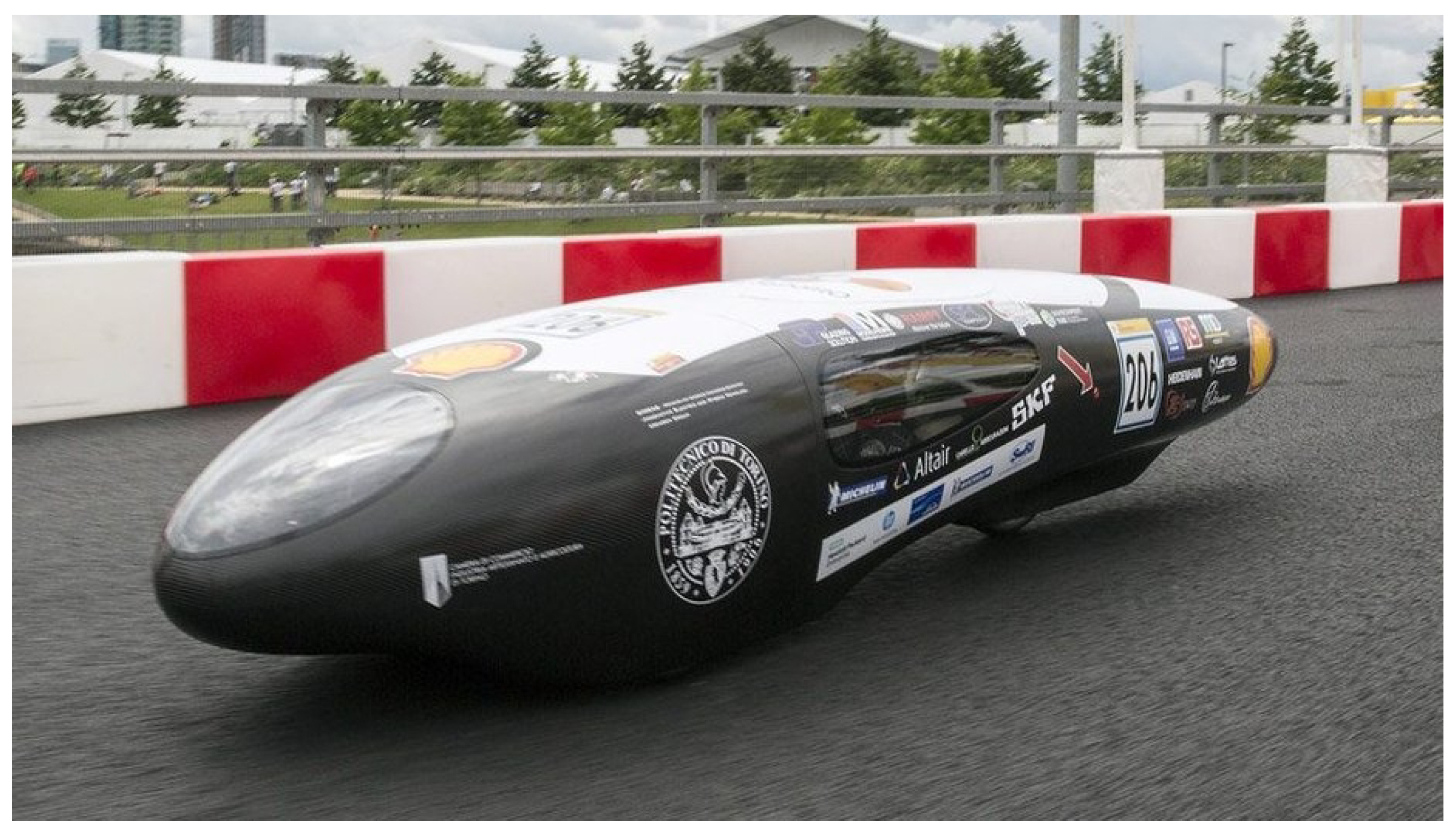
In this paper, building on the previous work presented in [15] in which preliminary results have been discussed, we present an original approach to EMS of a competition vehicle, studying the scenario in advance and solving an online optimization to drive the powertrain. The presented methodology eliminates the need to employ empirical techniques such as ‘Burn and Coast’, which typically involve human intervention through real-time adjustments during the run attempt. Furthermore, it extends the integration of MPC to vehicles equipped with hybrid energy storage while taking in to account the road inclination. In practice, we have considered the IDRAkronos vehicle (Figure 1) developed by Team H₂politO. Further details regarding the vehicle characteristics are presented in

Table A1. IDRAkronos vehicle parameters.

Quantity	Value
Maximum speed	35 km/h
Maximum range	60 km
Drag coefficient	0.088
Empty mass	39 kg
FC nominal power	500 W
DC motor nominal power	200 W

.

The next section presents the developed tank-to-wheel model and the results of the validation phase. Next, the vehicle speed profile optimization problem is formalized and solved. Finally, the cost function and constraints of the MPC are designed, the simulation results are discussed, and conclusions are drawn.

2. Problem Formulation

This paper presents an EMS for an FC vehicle equipped with a secondary PS. The SEM scenario is analyzed, and constraints on average vehicle speed and SC voltage are introduced. To enhance the effectiveness of the EMS design, it is assumed that all powertrain components remain unchanged.

As stated in the introduction, a point of paramount importance for obtaining an effective EMS is a high-fidelity model [16]. Accordingly, the next section presents the equations used for this purpose and the results of the model validation. After identifying the plant and scenario characteristics, the optimization problem is decomposed into two parts. The speed profile that minimizes the energy required to complete a full run attempt is found. When the optimal velocity profile is obtained, the controller tracks the reference state and solves the online power split problem between the main and secondary PS to ensure optimal fuel consumption.

The first step in the optimization process is to calculate the speed profile that the controller must track. This profile takes into account several factors, including the maximum allowed speed to prevent rollover in curves, the road gradient, and the maximum allowed armature current. To improve the robustness of the optimization process and ensure the reliability of the results, only the vehicle dynamics and the steady-state conditions of the electric motor are considered. The cost function used in the optimization is the integral of the armature current squared.

A nonlinear MPC algorithm with a binary optimization variable is used to control the plant. Fuel consumption optimization is achieved through the use of an appropriate cost function that selects the optimal PS to feed the powertrain. The arguments of the cost function are the FC current and the SC voltage. Additionally, the SC voltage is constrained to adhere to the SEM rules and ensure a valid run attempt.

All symbols used in the following are summarized in

Table A2. Variables.

Variable	Symbol	Unit
FC voltage	$V^{fc}$	V
FC current	$I^{fc}$	A
SC voltage	$V^{sc}$	V
SC current	$I^{sc}$	A
Armature voltage	$V^a$	V
Armature current	$I^a$	A
Rotor torque	$T^m$	Nm
Rotor speed	${\omega }^m$	rad/s
Driving torque	$T^d$	Nm
Slip speed	$\Delta \omega$	rad/s
Pinion torque	$T^p$	Nm
Pinion speed	${\omega }^p$	rad/s
Annular gear torque	$T^{ag}$	Nm
Annular gear speed	${\omega }^{ag}$	rad/s
Driving force	$F^d$	N
Vehicle speed	v	rad/s
Vehicle traveled distance	s	m
DC-DC duty cycle	$d^a$	-
Switching variable	$\Omega$	-
PS voltage	$V^{ps}$	V
PS current	$I^{ps}$	A

and 

Table A3. Parameters.

Parameter	Symbol	Unit
Open circuit voltage	$E_{oc}$	V
Number of cells	$N_c$	-
Tafel slope	A	V
Exchange current	$I_0$	A
Internal resistance	$R_{ohm}$	$\Omega$
SC capacitance	$C_{sc}$	F
Armature inductance	$L_a$	H
Armature resistance	$R_a$	$\Omega$
Speed constant	$k_e$	rad/sV
Torque constant	$k_t$	Nm/A
Rotor inertia	$J_m$	kgm2
DC motor driver efficiency	${\eta }_a$	-
Freewheel coefficients	$a,b,c$	-
Transmission ratio	$i_t$	-
Annular gear teeth	$n_{ag}$	-
Pinion teeth	$n_p$	-
Transmission efficiency	${\eta }_t$	-
Vehicle equivalent mass	$m_{eq}$	kg
Air density	${\rho }_{air}$	kg/m3
Frontal area	S	m2
Drag coefficient	$c_x$	-
Vehicle mass	m	kg
Gravitational acceleration	g	m/s2
Road inclination	$\alpha$	rad
Asymptotic rolling resistance coefficient	${\mu }_0$	-
Rolling radius	$r_r$	m
Threshold speed	$v_{th}$	m/s
Maximum speed	$v_{max}$	m/s
Number of phases	$N_{phase}$	-
Maximum armature current	$I_{max}^a$	A
Track length	$l_{track}$	m
Sample time	$T_s$	s
Prediction horizon	$H_p$	-
Scailing factor	$\gamma$	A/V
Recharge current	$I_{rch}$	A
Average vehicle speed	$v_{avg}$	m/s
Minimum allowed SC voltage	${\overline{V}}_{sc}^{min}$	V

for the variables and the parameters, respectively. The subscript i is used to indicate the phase in the offline optimization design and the symbol k is used to denote the time variable used to formulate the discrete-time controller.

3. Tank-to-Wheel Model

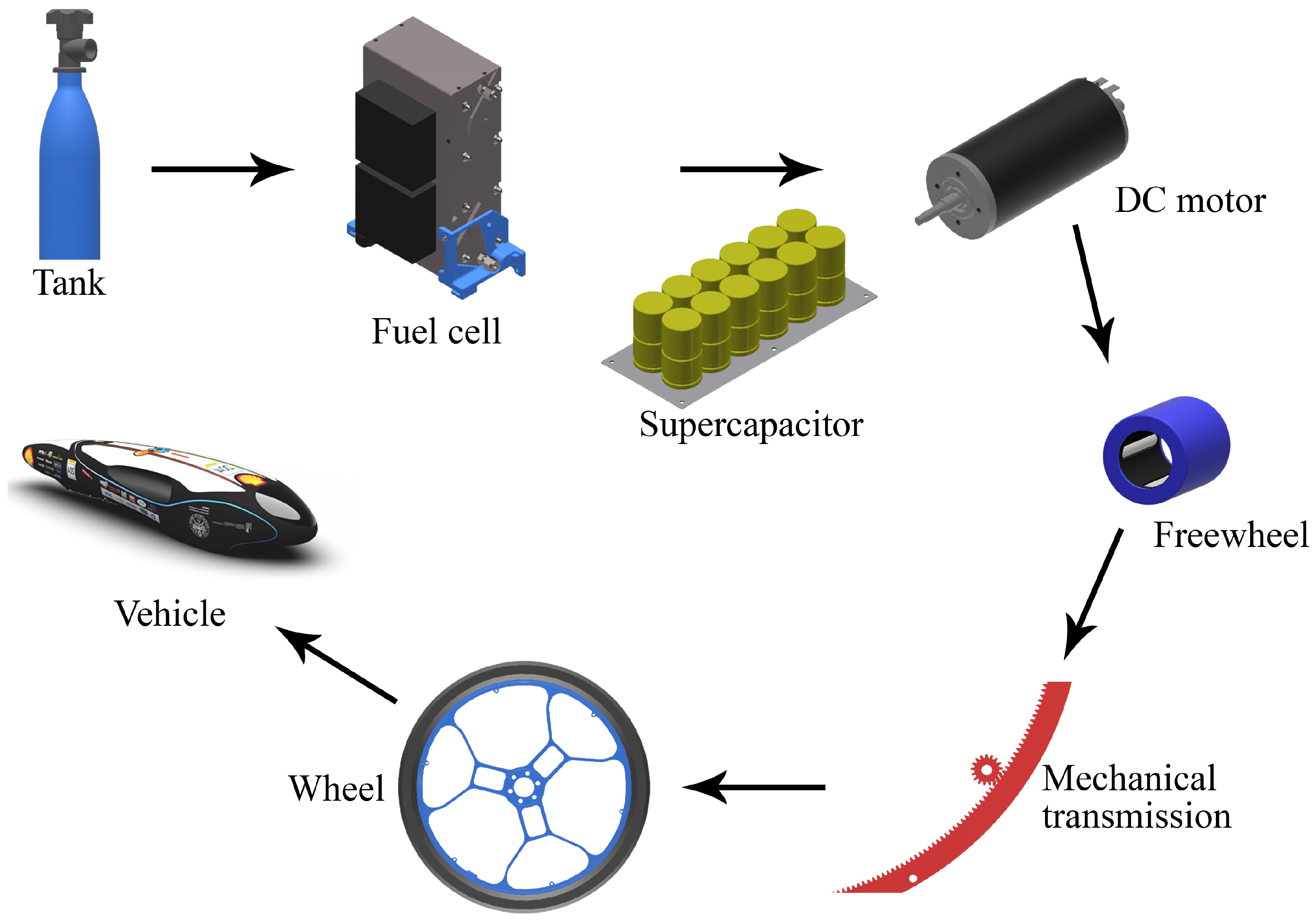
Figure 2 shows the powertrain components of the IDRAkronos; as mandated by the SEM rules [8], these are situated in the energy compartment, which is separated from the driver’s compartment by a bulkhead. The energy compartment contains all the electronic boards and microcontrollers needed for the powertrain.

The FC uses the hydrogen stored in the tank to produce electrical energy. The generated power can be used to supply the EM or to recharge the SC. Torque is applied to the vehicle’s rear drive wheel by a suitable mechanical transmission. In addition, a freewheel is inserted between the electric motor’s shaft and the mechanical transmission to decouple the system when the vehicle is free-rolling.

3.1. Equation Model

Using the simplified FC model described in [17], the generator can be modeled as a current-controlled ($I^{fc}$) voltage source ($V^{fc}$) as reported in Equation (1).

$$V^{fc}\left(I^{fc}\right)=E_{oc}-N_{c}Aln\left(\frac{I^{fc}}{I_0}\right)-R_{ohm}{I}^{fc}$$

(1)

The linear differential Equation (2) is used to evaluate the SC voltage $V^{sc}$ as a function of its current $I^{sc}$. The current $I^{sc}$ is assumed to be positive if the FC recharges the energy storage and negative if the SC feeds the electric motor.

$${\dot{V}}^{sc}=\frac{d{V}^{sc}}{dt}=\frac{I^{sc}}{C_{sc}}$$

(2)

The behavior of the brushed DC electric motor is described by two suitable equivalent circuits and the datasheet’s parameters ($L_a$, $R_a$, $k_e$, $k_t$, $J_m$). The linear differential Equations (3) and (4) evaluate the DC motor armature current $I^a$ and rotor speed ${\omega }^m$, respectively.

$${\dot{I}}^a=\frac{d{I}^a}{dt}=\frac{V^a}{L_a}-\frac{R_a}{L_a}{I}^a-\frac{k_e}{L_a}{\omega }^m$$

(3)

$${\dot{\omega }}^m=\frac{d{\omega }^m}{dt}=\frac{k_t}{J_m}{I}^a-\frac{T^m}{J_m}$$

(4)

The freewheel introduces a discontinuity in the plant behavior. The device is engaged if the rotor speed is greater than that of the mechanical transmission, and is disengaged otherwise. Exploiting the hyperbolic tangent function, the transmitted torque $T^d$ (6) is computed as a function of the slip $\Delta \omega$ between the two components (5).

$$\Delta \omega ={\omega }^m-{\omega }^p$$

(5)

$$T^d(\Delta \omega )=a[tanh(\Delta \omega -b)+c]$$

(6)

The mechanical transmission consists of a pinion and an annular gear. The system can be described using the transmission ratio $i_t$ reported in Equation (7). Under the assumption of constant efficiency ${\eta }_t$, the input torque $T^p$ and output torque $T^{ag}$ are linked as highlighted in Equation (8).

$$i_t=\frac{n_{ag}}{n_p}=\frac{{\omega }^p}{{\omega }^{ag}}$$

(7)

$$T^{ag}={\eta }_t{i}_t{T}^p$$

(8)

The vehicle model is studied taking into account only the longitudinal vehicle dynamic behavior described in Equations (9) and (10). Three different resistive force contributions are considered: the aerodynamic dragging force ($F^{aero}$) (11), the climbing force ($F^{climb}$) (12), and the rolling resistance force ($F^{roll}$) (13).

$$\dot{v}=\frac{dv}{dt}=\frac{F^d-F^{aero}-F^{climb}-F^{roll}}{m_{eq}}$$

(9)

$$\dot{s}=\frac{ds}{dt}=v$$

(10)

$$F^{aero}=\frac{1}{2}{\rho }_{air}S{c}_x{v}^2$$

(11)

$$F^{climb}=mgsin\alpha$$

(12)

$$F^{roll}=\mu mgcos\alpha$$

(13)

The driving force is computed assuming a constant rolling radius $r_r$ (14). To improve the model’s robustness, the tire rolling resistance coefficient $\mu$ is described by the asymptotically constant formulation in Equation (15).

$$F^d=\frac{T^{ag}}{r_r}$$

(14)

$$\mu ={\mu }_{0}tanh\left(\frac{v}{v_{th}}\right)$$

(15)

3.2. Model Validation

In order to obtain useful results from the equation model proposed in Section 3.1, the model parameters must be properly chosen. Information such as Computational Fluid Dynamics (CFD) simulations, Computer-Aided Design (CAD) tools, and manufacturing data can be used for this purpose.

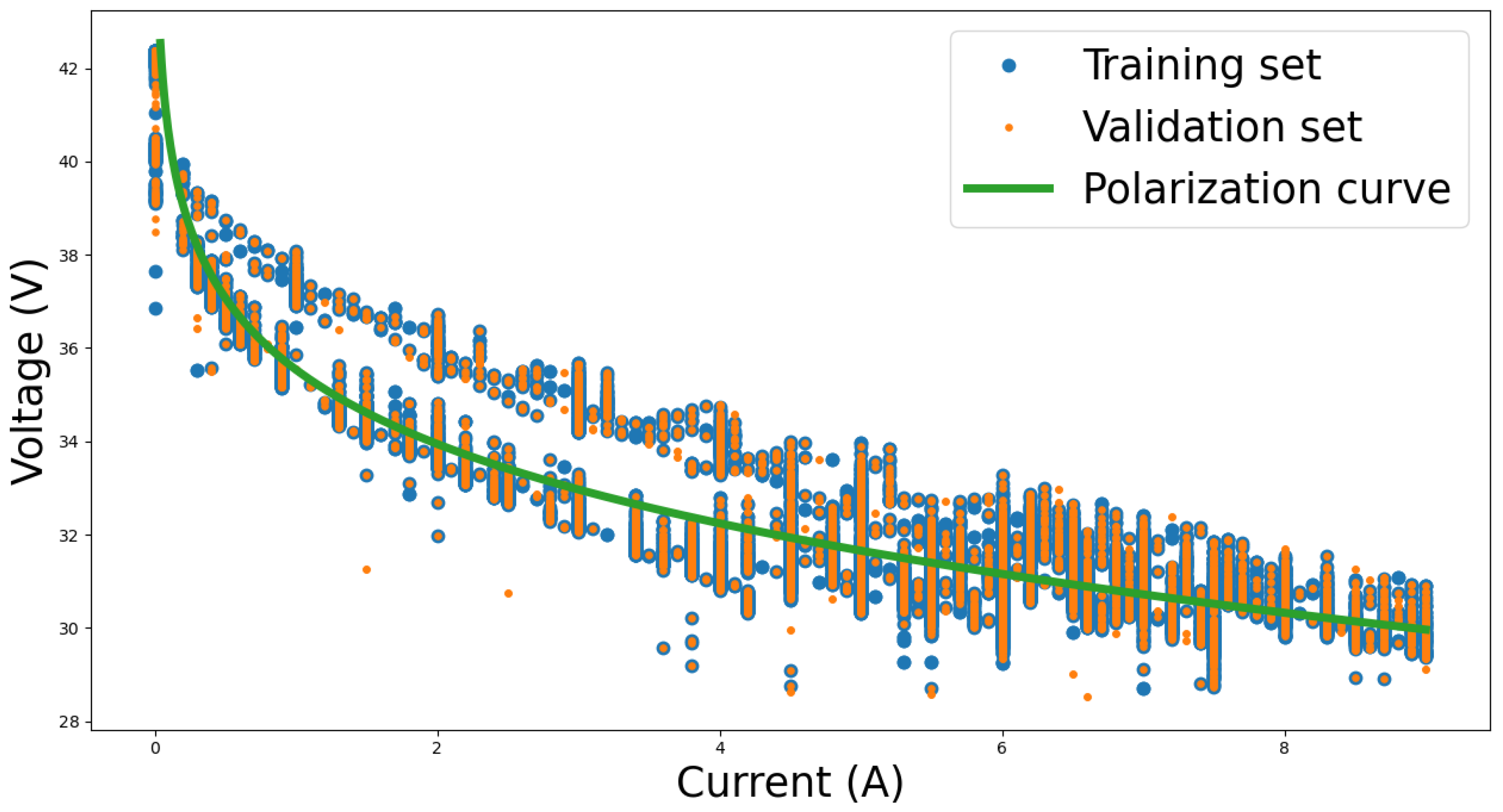
One of the most important aspects of overall powertrain efficiency relates to the FC electric model. As highlighted in the literature, FC efficiency is strongly influenced by aspects such as environmental conditions and power degradation. For this reason, we have chosen to estimate the internal resistance and Tafel slope through on-bench data. By rewriting Equation (1) in the form shown in Equation (16), the estimation problem is reduced to a least squares regression problem.

$$V^{fc}-E_{oc}=\left[\begin{array}{cc}A& R_{ohm}\end{array}\right]\left[\begin{array}{c}-N_{c}log\left(\frac{I^{fc}}{i_0}\right)\\ -I^{fc}\end{array}\right]$$

(16)

As shown in Figure 3, the data collected during the on-bench test were divided into two sets, with first used to estimate the unknown parameters and the second to validate the proposed model. The resulting polarization curve accurately characterizes the FC behavior and agrees well with the validation dataset, confirming the reliability of the model in simulating system responses.

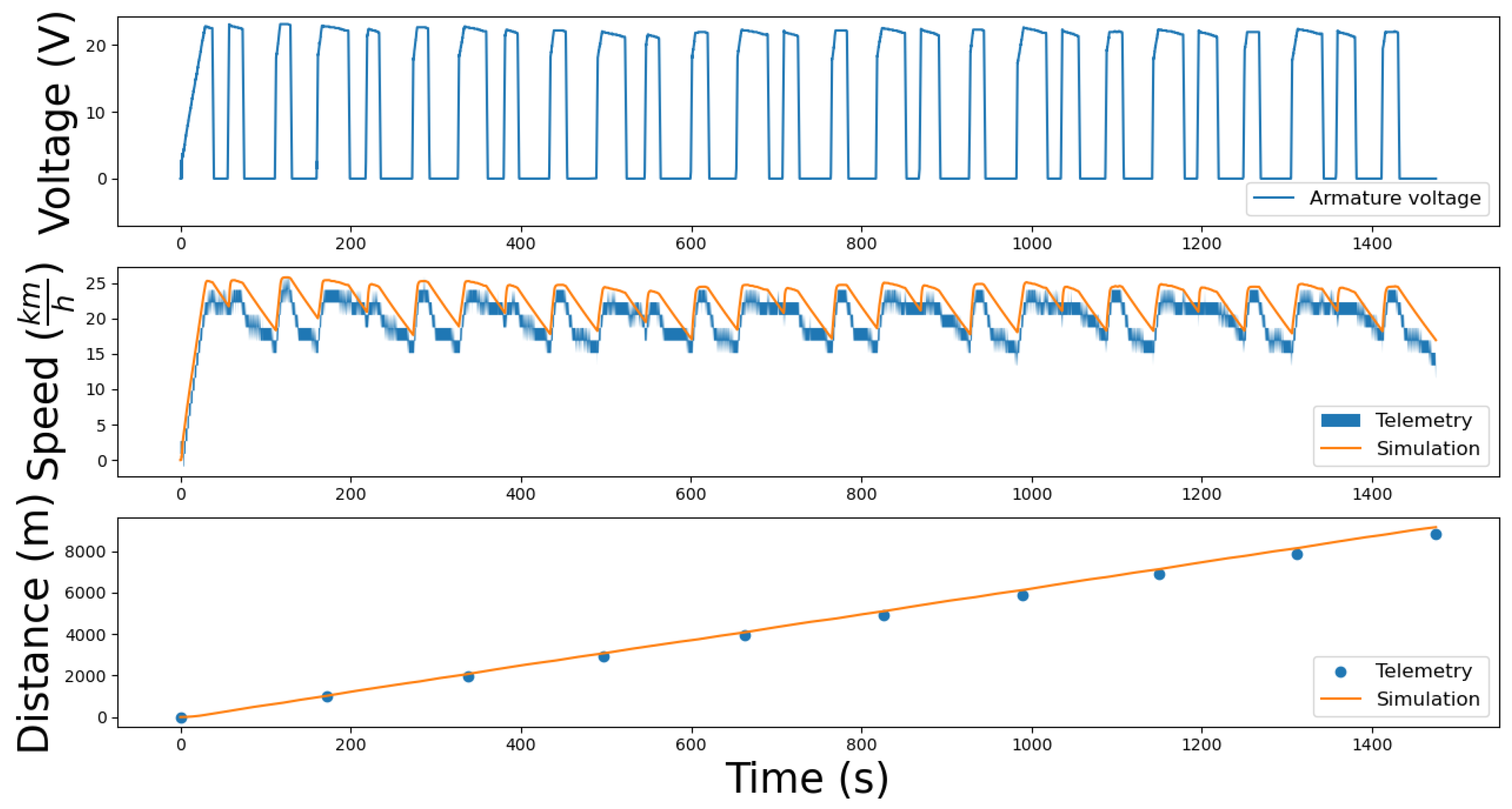
The vehicle’s dynamic parameters were gathered instead from a variety of sources: CFD simulation, wind tunnel testing, CAD analysis, and direct measurement. The resulting model was validated by comparing the simulation results with data collected on the track by an onboard data logger. In particular, the measured armature motor voltage was used as model input and vehicle speed and traveled distance were compared. Figure 4 highlights the model’s ability to describe the on-track data.

4. Reference Speed Profile Optimization

In this study, the scenario is assumed to be known. In particular, the information about the race track that hosts the SEM is available and can be studied in advance. For this reason, the first step in the proposed EMS is to compute a speed profile that minimizes the energy used to complete a run attempt. Specifically, the Circuit Paul Armagnac in Nogaro, France, where SEM 2022 took place, was analyzed.

Due to the nonlinear behavior of the freewheel and the impossibility of forecasting weather conditions, the plant model is simplified during this phase; the FC and the SC are neglected and the electric motor is studied in steady-state conditions. The simplified plant is described by two differential Equations (17) that have as states the vehicle speed and the traveled distance, respectively; the electric motor armature current is the plant input.

$$\begin{array}{cc}\hfill \dot{v}=\frac{{\eta }_t{i}_t{k}_t}{r_r{m}_{eq}}{I}^a-\frac{{\rho }_{air}S{c}_x}{2m_{eq}}{v}^2& -\frac{mg}{m_{eq}}({\mu }_{0}cos\alpha +sin\alpha )\hfill \\ \hfill \dot{s}& =v\hfill \end{array}$$

(17)

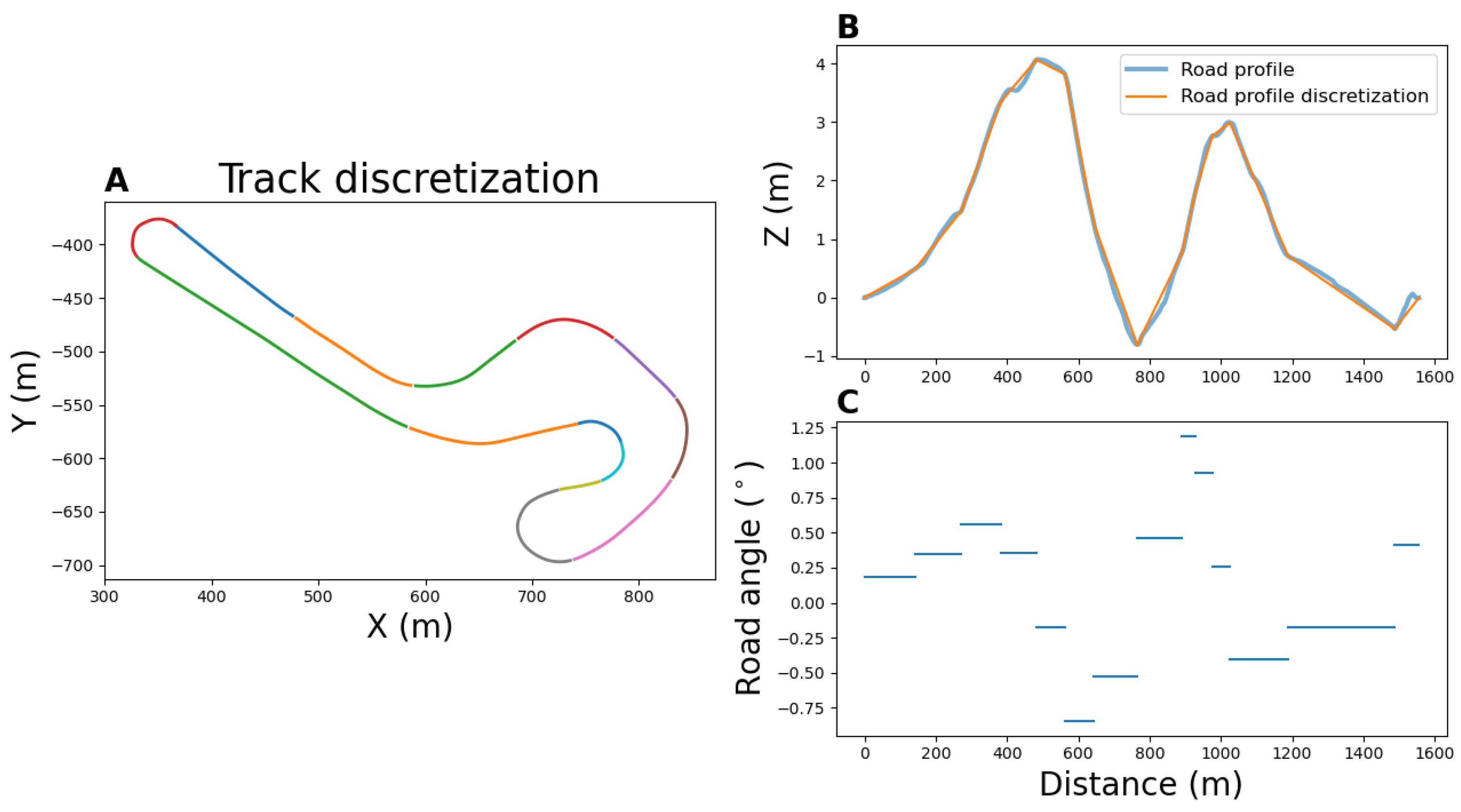
Because of its low mass and low-drag characteristics, the IDRAkronos vehicle is highly sensitive to the road slope. Thus, the track elevation must be taken into account during the offline optimization process. The circuit track (Figure 5) is designed through a multi-phase approach composed of $N_{phase}$ tracts. The track elevation is represented as a linear piecewise function. The sectors are defined according to two criteria: constant turning radius (Figure 5A) and constant road gradient (Figure 5B,C).

The energy optimization problem is formalized through a cost function that aims to minimize the armature current energy associated with Equation (18).

$$\begin{array}{cc}\hfill \underset{I^a}{min}& {\int }_{t_0}^{t_{end}}{\left(I^a\right)}^2\left(t\right)dt\hfill \end{array}$$

(18)

$$\begin{array}{cc}\hfill \mathrm{s}.\mathrm{t}.& s_i^{end}=s_{i+1}^{0}i\in \{1,\dots ,N_{phase}-1\}\hfill \end{array}$$

(19)

$$\begin{array}{cc}& v_i^{end}=v_{i+1}^{0}i\in \{1,\dots ,N_{phase}-1\}\hfill \end{array}$$

(20)

$$\begin{array}{cc}& v_i\left(t\right)\le v_i^{max}i\in \{1,\dots ,N_{phase}\}\hfill \end{array}$$

(21)

$$\begin{array}{cc}& 0\le I^a\left(t\right)\le I_{max}^a\hfill \end{array}$$

(22)

$$\begin{array}{cc}& s\left(t_0\right)=0v\left(t_0\right)=0\hfill \end{array}$$

(23)

$$\begin{array}{cc}& s\left(t_{end}\right)=l_{track}\hfill \end{array}$$

(24)

$$\begin{array}{cc}& \frac{l_{track}}{t_{end}-t_0}\ge 25\mathrm{km}/\mathrm{h}\hfill \end{array}$$

(25)

To ensure the feasibility of the optimization process and prioritize driver safety, several constraints are introduced. Equations (19) and (20) guarantee state continuity, Equation (21) prevents the vehicle from entering a rollover condition, and the mathematical inequalities in Equation (22) avoid overfeeding of the DC motor and negative armature current. Equation (23) enforces the initial state condition, while Equation (24) defines the desired final state value. Additionally, the average vehicle speed is constrained to meet the SEM rules, establishing a lower bound described by Equation (25). The formulated problem is a multi-phase nonlinear optimization problem. MATLAB software GPOPS 5.0 [18] was used to solve the optimization problem.

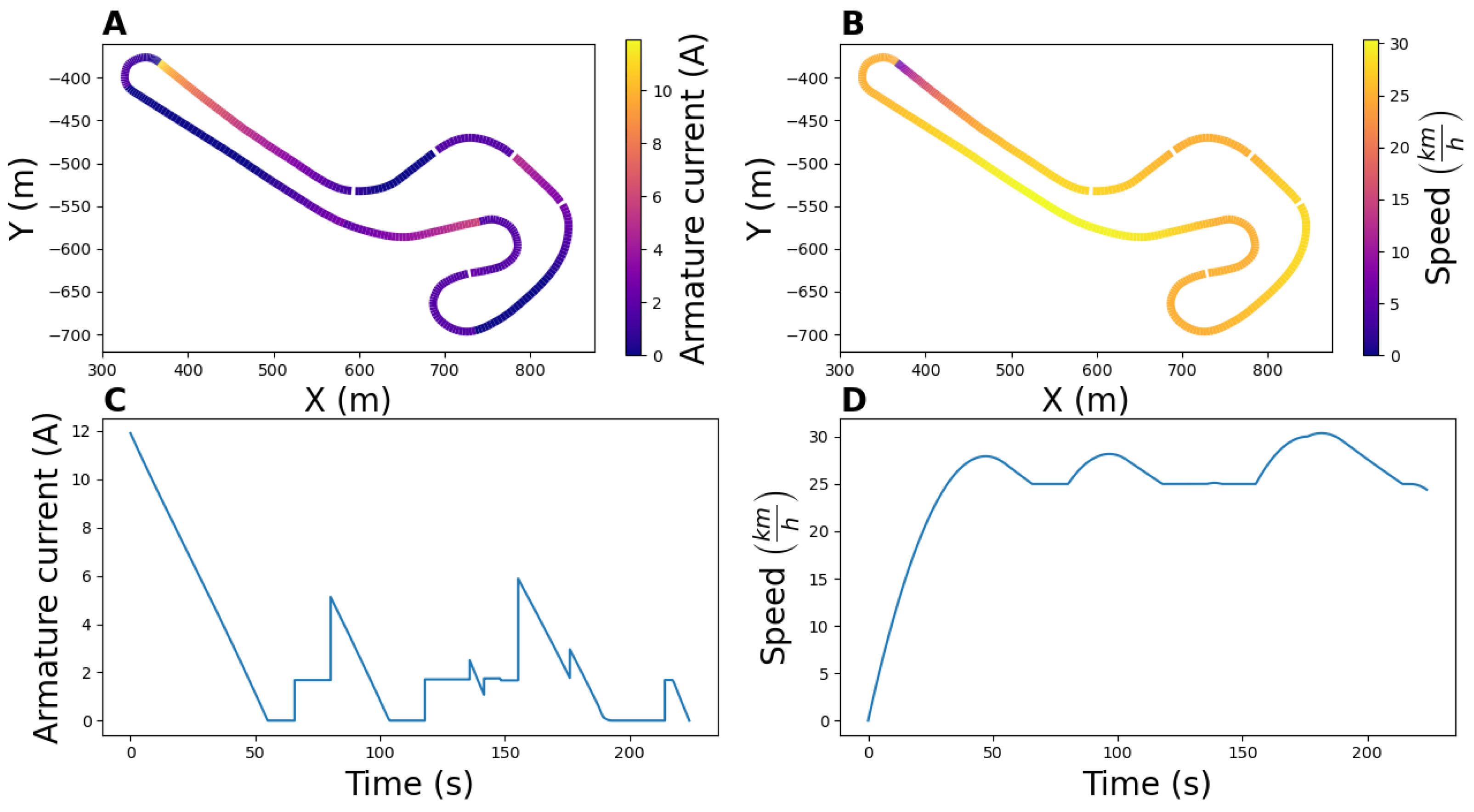
The obtained results are depicted in Figure 6. In particular, the current profile that minimizes the cost function is presented in Figure 6A,C and the optimal speed profile that fulfills the constraints is evaluated in Figure 6B,D.

5. MPC Design for Energy Management

In this section, the energy management problem is formulated and solved. To design the controller and predict the plant state at the next time instant, the equations presented in Section 3.1 are discretized through the forward Euler method and linearized where necessary.

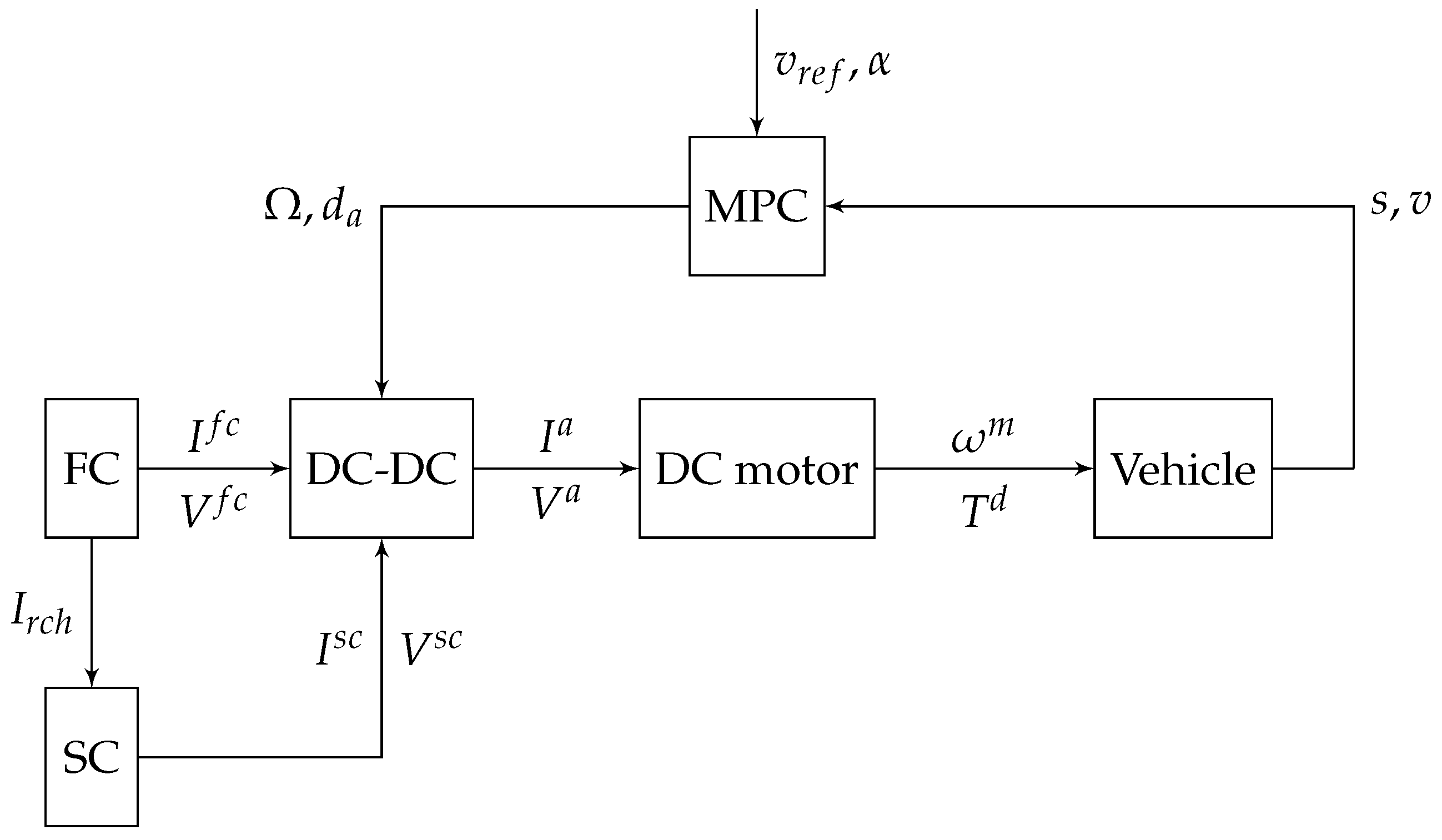
Figure 7 shows the developed system block diagram used to design the controller. In this design’s encapsulated architecture, the MPC operates at a higher level; consequently, the DC–DC pass bandwidth is kept wider than that of the MPC during the design process.

The plant states are the vehicle speed v and the traveled distance s, while the DC–DC converter duty cycle $d^a$ and the switching variable $\Omega$ are the inputs. The former determines the duty cycle of the brushed motor driver and, based on the powertrain PS voltage, the armature voltage $V^a$, while the latter defines the power supply of the driveline (i.e., FC or SC).

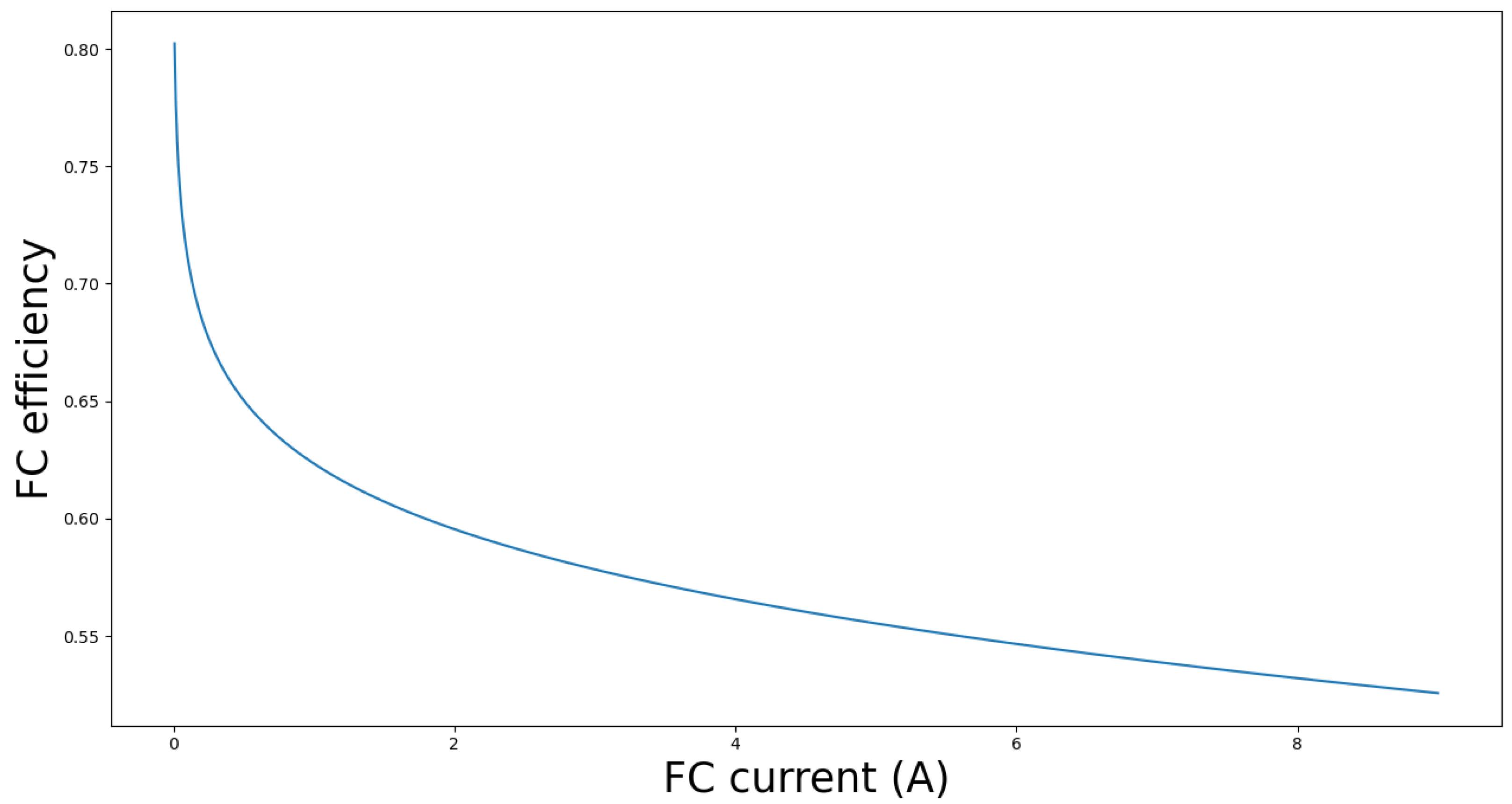
The goal of the designed controller is to optimize the hydrogen consumption of the vehicle. The efficiency of the FC decreases significantly as the drawn current increases (Figure 8); hence, the controller must be able to properly select the power source of the powertrain. Appropriate usage of the SC can overcome FC performance degradation and reduce fuel consumption.

The cost function (26) optimizes the vehicle’s fuel consumption while taking into account the fuel cell current $I^{fc}$ and the SC voltage $V^{sc}$ by acting on the binary control variable $\Omega$. According to the working principle of a proton exchange membrane fuel cell, the supplied current is linearly proportional to its consumption. On the other hand, by exploiting the SC’s recharge architecture, the hydrogen used in this task can be approximated by a linear function of the SC voltage $V^{sc}$. The scaling factor $\gamma$ is introduced to equalize the two quantities (i.e., $I^{fc}$ and $V^{sc}$). In addition, the SEM rules require that the SC voltage at the end of the run must be equal to that measured at the starting line.

Exploiting Equation (2) and assuming constant current recharge, the optimization constraint is formulated in Equation (27).

$$\begin{array}{cc}\hfill \underset{\Omega }{min}& \sum _{k=1}^{H_p}\Omega {\left(I_k^{fc}\right)}^2+(\Omega -1){\left(\gamma V_k^{sc}\right)}^2\Omega \in \{0,1\}\hfill \\ \hfill \mathrm{s}.\mathrm{t}.& V_k^{s{c}^{*}}={\overline{V}}_{sc}-\frac{I_{rch}}{C_{sc}}\frac{l_{track}-s_k}{v_{avg}}\hfill \end{array}$$

(26)

$$\begin{array}{cc}& V_k^{sc,low}=\left\{\begin{array}{cc}{V}_k^{s{c}^{*}}\hfill & \mathrm{if}{V}_k^{s{c}^{*}}\ge {\overline{V}}_{sc,min}\hfill \\ {\overline{V}}_{sc,min}\hfill & \mathrm{otherwise}\hfill \end{array}\right.\hfill \end{array}$$

(27)

The first term of the cost function, $I^{fc}$, is affected by two factors, namely, the current supplied to the armature $I^a$ and the current used to charge the SC $I^{rch}$. The first is evaluated based on the known state of the DC motor, while the second exploits a linearized model of the FC’s behavior (28). In addition, in order to simplify the computation, the FC voltage $V^{fc}$ is assumed to be constant within the prediction horizon.

$$\left\{\begin{array}{cc}{I}_k^{fc}=I_k^a{d}_k^{a,fc}\hfill & \mathrm{if}\mathrm{SC}\mathrm{not}\mathrm{recharged}\hfill \\ I_k^{fc}=I_k^a{d}_k^{a,fc}+(\beta V_k^{sc}+\delta )\hfill & \mathrm{otherwise}\hfill \end{array}\right.$$

(28)

The supercapacitor voltage (30) is predicted by the SC net current $I^{sc}$ (29).

$$\left\{\begin{array}{cc}{I}_k^{sc}=-I_k^a{d}_k^{a,sc}\hfill & \mathrm{if}\mathrm{SC}\mathrm{not}\mathrm{recharged}\hfill \\ I_k^{sc}=-I_k^a{d}_k^{a,sc}+I_{rch}\hfill & \mathrm{otherwise}\hfill \end{array}\right.$$

(29)

$$V_{k+1}^{sc}=\frac{I_k^{sc}}{C_{sc}}{T}_s+V_k^{sc}$$

(30)

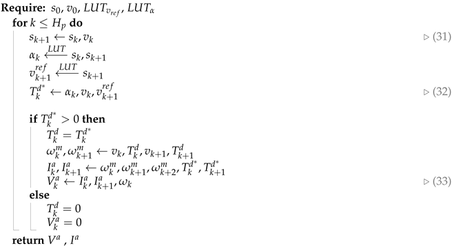
As highlighted in Equations (28) and (30), the terms of the cost function depend on the DC motor’s armature current. Therefore, the state of the electric motor must be predicted to evaluate Equation (26). For this purpose, at each sample time, the prediction of the vehicle position is computed one step ahead (31) and this information is used to forecast the reference vehicle speed on the basis of a suitable Look-Up Table (LUT).

$$s_{k+1}=v_k{T}_s+s_k$$

(31)

Under the assumption of a known scenario, the road profile slope $\alpha$ can be predicted by a proper LUT; thus, the necessary driving torque needed to track the optimal speed profile can be computed using Equation (32).

$$\begin{array}{c}\hfill T_k^{d^{*}}=\left[\frac{v_{k+1}^{ref}-v_k}{T_s}+\frac{{\rho }_{air}S{c}_x}{2m_{eq}}{v}_k^2\right.\\ \hfill \left.+\frac{mg}{m_{eq}}\left({\mu }_{0}cos{\alpha }_k-sin{\alpha }_k\right)\right]\frac{m_{eq}{r}_r}{{\eta }_g{i}_g}\end{array}$$

(32)

The presence of the freewheel prevents the application of negative driving torque; therefore, the electric motor is switched off if the computed torque is less than zero (i.e., $V^a=0$). Conversely, Equation (33) is used to determine the voltage of the DC motor $V^a$.

$$V_k^a=\left(\frac{I_{k+1}^a-I_k^a}{T_s}+\frac{R_a}{L_a}{I}_k^a+\frac{k_e}{L_a}\right)L_a$$

(33)

Through the DC–DC duty cycle (34), the armature state is linked to the voltage $V^{ps}$ and the current $I^{ps}$ of the power source.

$$d_k^a=\frac{V_k^a}{V_k^{ps}}=\frac{I_k^{ps}}{I_k^a}{\eta }_a$$

(34)

To predict the system state at the next instant, it is assumed that the vehicle properly tracks the reference speed profile. As a result, the proposed Algorithm 1 can be used iteratively until the end of the run attempt.

Algorithms 1 and 2 summarize the steps required to calculate the control action. The DC motor states are defined as a function of the required drive torque needed to follow the reference speed profile. The optimal input sequence is obtained by evaluating the cost function over the prediction horizon and taking care to satisfy the constraints.

Algorithm 1 Armature state prediction algorithm.

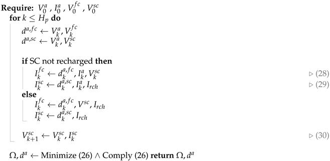
Algorithm 2 EMS algorithm.

6. Testing and Simulations

Extensive simulations were performed to evaluate the proposed EMS. Two different scenarios were used to evaluate the performance of the designed solution. The first, referred to as the simplified scenario, consisted of only one lap of the Circuit Paul Armagnac in Nogaro, France, with a length of 1571 m, and was used to analyze the influence of different factors on the performance. The second, called the full scenario, consisted of ten laps (15,710 m) and aimed to simulate an effective race test.

The MPC utilizes a prediction horizon of 2 and operates with a sampling time of 0.5 s. The latter selection ensures that the EMS operates at a slower pace compared to the other powertrain controllers, such as the DC–DC driver and FC cooling fan. The optimal solution is computed using a brute-force approach that evaluates all possible combinations of the control sequence to determine the optimal result.

The scaling factor $\gamma$ is critical for the performance of the controller. A preliminary value of this parameter is estimated by calculating the relationship between the SC voltage and the FC current. This value is then adjusted in each simulation setup using a heuristic approach. The scaling factor is subjected to a gain between 13.3 and 3.6 with respect to the initial estimation.

Although the application of proper control logic to the SC recharging process influences hydrogen consumption [19], this aspect is not investigated in the present paper. In the simulation environment, the SC is recharged by a constant current if the SC voltage is below the target voltage. Moreover, due to the low powertrain efficiency in low-power regimes, the electric motor is turned off if the DC–DC duty cycle is below a certain threshold. If the SC voltage is lower than that required to properly supply the electric motor while following the reference speed profile, the optimization is bypassed and the FC is used as the PS.

The controller’s performance was evaluated using two different simulations with the same setup; in the first, only the FC was used to supply the powertrain, while in the second the designed MPC was used to perform EMS.

In the simplified scenario, the influence of different factors on the controller’s performance was evaluated, specifically, the impact of the prediction horizon on fuel saving and the potential delayed response of the FC. The results indicate that while an increase in the prediction horizon leads to higher computational time (approximately five times more), it does not provide significant performance improvements. On the other hand, there is an overall reduction in fuel consumption when a delay in the FC behavior is present. These findings can be attributed to the assumption of a constant FC voltage in the prediction horizon.

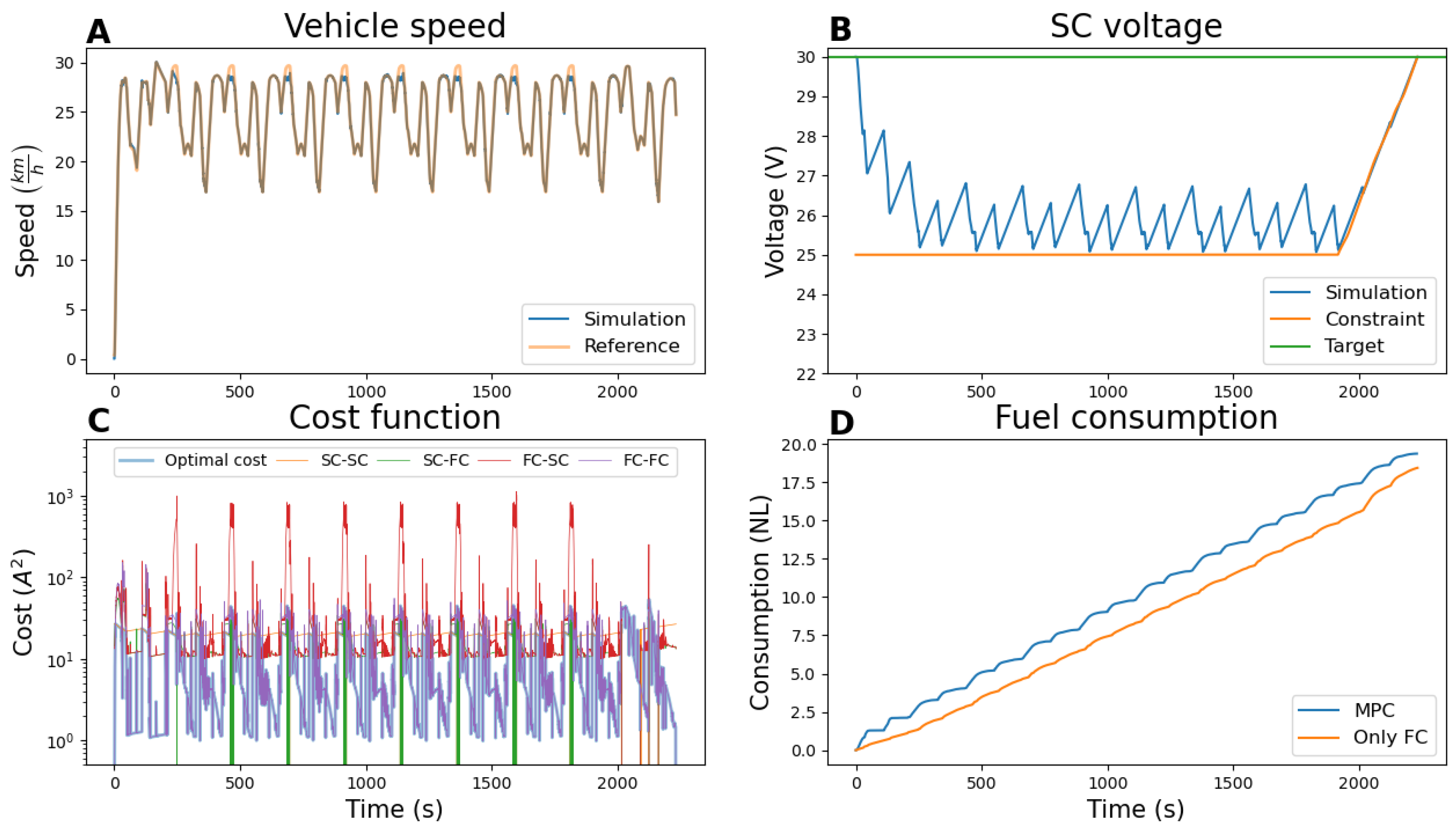
Figure 9 illustrates the results of a complete simulated SEM run. The plot in Figure 9A shows that the vehicle speed tracks the optimal speed profile computed during offline optimization. The graph in Figure 9C presents the control sequences computed by the MPC; due to the use of a binary switching variable and a prediction horizon equal to two at each sample time, four control sequences were ultimately evaluated. The control sequences that violate the constraints are marked with a negative cost function value. The plot in Figure 9B shows that the SC voltage at the end of the simulation is equal to that at the first time instant. From the figure, it is possible to appreciate that the secondary PS is crucial during the starting phase. The SC is discharged and provides the energy to put the vehicle in motion. This consideration is reinforced by the fuel consumption graph (Figure 9D). The two hydrogen consumption curves are generally parallel except at the beginning and end of the simulation. By introducing the designed MPC, the energy stored in the SC is used in the startup phase, resulting in the hydrogen consumption being lower than the benchmark.

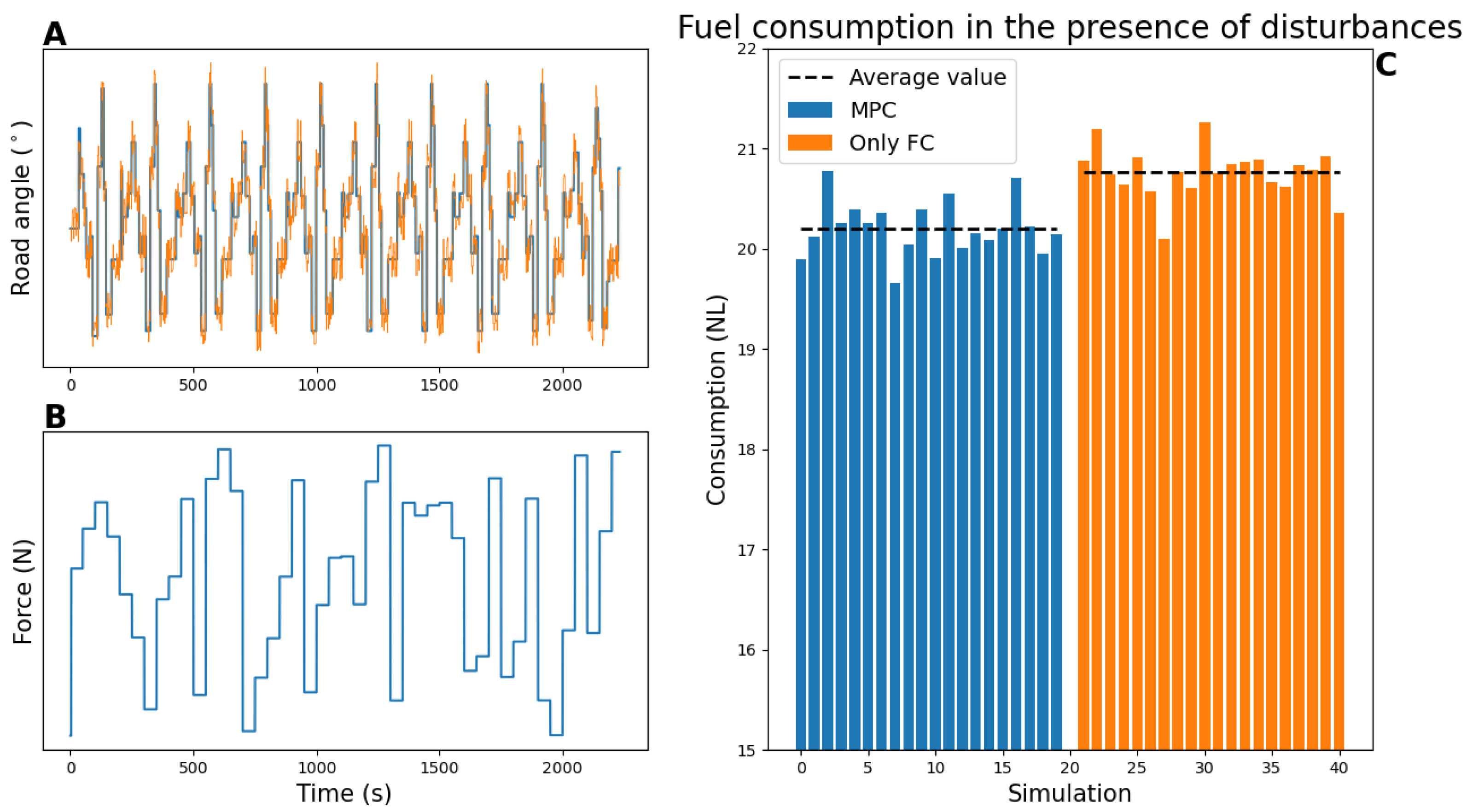
Next, disturbances were introduced to assess the controller’s robustness against unforeseeable events such as wind or traffic jams. Specifically, random noise with a mean value of zero and variance of 15% of the maximum road slope was added to the road profile inclination to simulate possible mismatches between the reference model and the real situation. A drag force was applied directly to the vehicle to simulate possible braking due to an unforeseen event (e.g., slower vehicles, traffic jams, yellow flags) or the presence of wind. The maximum force value can be traced back to a gust of wind that acts frontally on the vehicle with a speed of about 20 km/h. To evaluate the performance of the proposed solution in the presence of disturbances, forty simulations were carried out (Figure 10).

Table 1. Simulation results.

Set-Up			Consumption
Scenario	Test	$\gamma$	Only FC (NL)	MPC (NL)	Saving (%)
simplified	$H_p=2$	0.44	6.9	6.2	10.1
simplified	$H_p=3$	0.39	6.9	6.2	10.1
simplified	FC delayed	0.24	6.7	6.1	8.9
full	run attempt	0.12	19.4	18.4	5.1
full	disturbances	0.12	20.8	20.2	2.9

reports the average values of two sets of simulations. Random disturbances were introduced in the first set, composed of twenty simulations, while in the other twenty no disturbances were applied.

The last three columns of Table 1 show the performance of the controller in terms of fuel consumption and hydrogen savings for all of the considered setups. The simulation results demonstrate fuel savings from 2.9% to 10.1%. The presence of disturbances increases the total hydrogen consumption; nevertheless, a significant improvement is achieved.

7. Conclusions

This paper proposes a low-computational-cost EMS for FC hydrogen vehicles with a secondary power source. The proposed solution can effectively handle possible constraints on the secondary PS state at the end of the test, such as the SC voltage or the battery’s state of charge. The results obtained in the simulation phase highlight that the controller is able to reduce fuel consumption, handle constraints, and overcome the presence of disturbances.

To simplify the investigation, a well-known scenario was used in the study; this condition can be traced back to a driving cycle. Nevertheless, the architecture can be improved by the introduction of an online speed profile optimizer and a road profile estimator.

In future research, on-bench and on-track tests could be used to further validate the results. In addition, the control performance could be improved by exploring techniques such as MPC gain scheduling to increase the accuracy of online optimization or by developing a new DC motor driver capable of handling continuous commutation between the primary and secondary PSs.