Article

A Deep Learning Method for the Health State Prediction of Lithium-Ion Batteries Based on LUT-Memory and Quantization

by
Mohamed H. Al-Meer
Computer Science & Engineering Department, Qatar University, Doha 2713, Qatar
World Electr. Veh. J. 2024, 15(2), 38; https://doi.org/10.3390/wevj15020038
Submission received: 15 November 2023 / Revised: 29 December 2023 / Accepted: 17 January 2024 / Published: 24 January 2024
(This article belongs to the Special Issue Deep Learning Applications for Electric Vehicles)

Abstract

:
The precise determination of the state of health (SOH) of lithium-ion batteries is critical in the domain of battery management systems. The proposed model in this research paper emulates any deep learning or machine learning model by utilizing a Look Up Table (LUT) memory to store all activation inputs and their corresponding outputs. The operation that follows the completion of training is referred to as the LUT memory preparation procedure. This method’s lookup process supplants the inference process entirely and simply. This is achieved by discretizing the input data and features before binarizing them. The term for the aforementioned operation is the LUT inference method. This procedure was evaluated in this study using two distinct neural network architectures: a bidirectional long short-term memory (LSTM) architecture and a standard fully connected neural network (FCNN). It is anticipated that considerably greater efficiency and velocity will be achieved during the inference procedure when the pre-trained deep neural network architecture is inferred directly. The principal aim of this research is to construct a lookup table that effectively establishes correlations between the SOH of lithium-ion batteries and ensures a degree of imprecision that is tolerable. According to the results obtained from the NASA PCoE lithium-ion battery dataset, the proposed methodology exhibits a performance that is largely comparable to that of the initial machine learning models. Utilizing the error assessment metrics RMSE, MAE, and (MAPE), the accuracy of the SOH prediction has been quantitatively evaluated. The indicators mentioned above demonstrate a significant degree of accuracy when predicting SOH.

1. Introduction

The use of lithium-ion batteries has rapidly increased due to their low cost, high energy densities, low self-discharge rate, and long lifetime compared to other batteries [1,2,3,4]. Hence, lithium-ion batteries have gained significant prominence across diverse domains, including, but not limited to, mobile computing devices, aerospace applications, electric cars, and energy storage systems [5,6]. Despite the noteworthy advantages of lithium-ion batteries, a significant drawback is the occurrence of capacity fading upon repeated utilization. In addition, it is imperative to diligently observe and precisely assess their capacity, since an inaccurate evaluation of capacity might result in irreversible harm to the battery through excessive charging or discharging [7]. The assessment of battery capacity fade relies heavily on what is called the state of health, or SOH, serves as a pivotal indication of battery capacity. Hence, it is vital to precisely determine the SOH of lithium-ion batteries in order to ensure their safety and dependability [8].
Numerous research endeavors have been undertaken to obtain a precise assessment of the SOH of batteries. In general, the studies can be categorized into three distinct groups: model-based methods [9,10,11,12,13,14], data-driven methods [15,16], and hybrid methods [17,18].
The evaluation of a battery’s health state, as determined by the SOH metric, is conducted based on the varying beginning capacities of each battery. There exist several approaches for determining the SOH of a battery. However, the predominant methods revolve around assessing its impedance and its useful capacity. The utilization of the battery’s impedance as a measuring technique is deemed unsuitable for online applications due to the necessity of specialized instruments, for example electrochemical impedance spectroscopy. The majority of research therefore used the SOH metric, which is based on the battery’s usable capacity, to measure its performance.
The subsequent sections of this article are structured in the following manner: Section 1 outlines the many contemporary techniques employed for forecasting the state of health (SOH) of batteries. Section 2 presents the employed approach and its corresponding context. Section 3 enumerates other relevant studies. Section 4 provides a comprehensive summary of the dataset utilized. Section 5 demonstrates the utilization of the FCNN and LSTM training models. Section 6 of the paper focuses on the assessment of performance and the specific measurements employed. Discussions on the study’s results are presented in Section 7. In Section 8, the conclusion is represented.
Numerous studies have been undertaken to precisely assess the state of health (SOH) of batteries. The methods can be categorized into three distinct groups: direct measurement (experimental) methods, model-based methods, and data-driven methods.
Starting with the experimental methods, cycle counting determines the age of a battery by analyzing its chronological charge and discharge cycles. The most straightforward approach to determine the SOH is by tallying the total number of battery cycles. During each cycle, the degradation of batteries is significantly influenced by characteristics such as charge and discharge depth temperatures, as well as their C rating. A coefficient can be derived to establish a connection between those characteristics and the full discharge (100% depth of discharge) [19].
Charge counting: The charge counting method, also known as ampere-hour counting, is regarded as a precise and straightforward approach for measuring battery capacity. The ratio of the actual battery capacity (Qact) to its nominal capacity (Qnom) yields an accurate SOH. The measurement of the charge transferred throughout a complete charging or discharging process at a low C-rate and controlled temperature (usually 25 °C) provides a precise assessment of the remaining capacity [19,20,21].
S O H = Q a c t Q n o m
The internal resistance approach is based on the observation that the internal resistance (IR) of a battery increases as it ages. This property makes it a good parameter for estimating the SOH of a battery. To compute the IR, one can take a small step in the current and apply Ohm’s law, as shown in Equation (2). Here, ∆Ut represents the voltage pulse and ∆UL represents the current pulse [19,20].
R 0 = U t U L
The electrochemical impedance spectroscopy (EIS) method involves analyzing the impedance properties of a battery by subjecting it to a sinusoidal current voltage signal across a broad range of frequencies. Consequently, the response of a current or voltage can be examined. A Nyquist plot can facilitate comprehension of the estimation. Furthermore, Warburg elements, in addition to inductors, can be used in an ECM to enhance the capture of intricate dynamics. At low frequencies, the impedance is essentially ohmic, and the significance of capacitive effects increases. The ohmic resistance exhibits a direct relationship with battery aging, therefore making it a suitable indicator for SOH assessment [19]. Despite its accuracy, this system is deemed challenging to apply due to its high cost and complexity.
The Incremental Capacity Analysis (ICA) method examines the rate of change of the charge Q in relation to the voltage V. The morphology of the IC curve undergoes alterations as it ages, rendering it a potential predictor of the SOH. As the battery degrades, the incline of the voltage curve during the constant current charging phase intensifies. The primary drawbacks of the ICA technique are the requirement for a relatively low C-rate compared to typical charge rates and the computationally intensive numerical differentiation carried out by the BMS.
The differential voltage analysis method (DVA) [22] shares similarities with the Independent Component Analysis (ICA) method. The rate of change of voltage, denoted as V, with respect to the charge, is calculated during the constant current (CC) charging phase. The peaks in question correspond to specific chemical reactions within the cell that persist independent of battery aging. The gap between these peaks indicates a segment of the battery’s capacity that can be utilized for estimating its SOH.
The inside examination of a battery cell, without causing any harm, can be accomplished by employing ultrasonic inspection or X-ray techniques. Both tasks can be executed manually during maintenance in order to obtain an approximation of its SOH. The idea relies on the sensitivity of ultrasonic wave propagation in liquid-filled porous media to several factors such as electrode tortuosity, porosity, thickness, density, elastic modulus, fluid density, and ion concentration [23,24]. A more thorough comprehension of the aging process in different types of batteries has been achieved using techniques such as X-ray computed tomography [25] and others [26]. Characterizing the internal information with accuracy can be a difficult undertaking; the fundamental aging mechanisms must be deduced from the examination of exterior signals. Several studies integrate ultrasonic examination and machine learning to accurately evaluate the SOH.
A battery SOH estimation can be achieved by a number of model-based approaches, which entail building a model of a battery and including the internal deterioration process in the model. Knowledge of the internal battery reaction mechanisms, the accurate formulation of the mathematical equations driving these reactions, and the development of effective simulation models are all essential for model-based approaches. There may be difficulties in putting these ideas into practice. Lithium-ion battery life was predicted using a weighted ampere-hour throughput model in a study by the author in [27]. The researcher determined how severely the batteries had been damaged. To determine a battery’s SOH, the author of [28] applied an analog circuit model and an improved Kalman filter. To determine a battery’s SOH, in the study presented in [29], the authors relied on nominal filtering methods. They discovered that battery capacity is proportional to the square of the internal impedance. The researchers in [30] presented a method for estimating a battery’s SOH, or state of health. This method takes battery discharge rates as input variables for a state-space model. The SOH of a battery was predicted using a single-particle model developed by study [31], which is based on the physics of electrolytes. The degeneration of the internal mechanisms and the batteries were the focus of this investigation. From a chemical perspective, the construction of a precise aging model for lithium-ion batteries is difficult due to the complex structure of the chemical interactions occurring within the battery, although model-based approaches are useful in forecasting the SOH of batteries. Furthermore, various environmental variables, such as operational temperature, anode and cathode materials, and related parameters, have a major impact on the performance of lithium-ion batteries. Therefore, there are difficulties in establishing a reliable aging model for lithium-ion batteries.
Improvements in hardware have allowed computers to perform increasingly complex mathematical operations in recent years. Concurrently, there has been an uptick in the number of databases that can be mined for information on a battery’s SOH due to the growing use of data-driven methodologies for this purpose. This paved the way for the broad adoption of data-driven approaches. Even without a thorough understanding of the battery’s internal structure and aging mechanisms from an electrochemical standpoint, a data-driven method allows for the reliable prediction of a battery’s SOH. Therefore, these methods can be implemented with little to no familiarity with a battery’s electrochemical properties or the environmental context. The success of data-driven approaches relies greatly on the accuracy and usefulness of the information that is collected. Acquiring attributes that are highly linked with the degradation process is crucial to the success of a data-driven model. In a related study [32], the authors suggested using sparse Bayesian predictive modeling with a sample entropy metric to boost the reliability of voltage sequence predictions. The SOH of a battery can be estimated and analyzed with the help of a hidden Markov model, which was introduced by the authors in study [33]. In a different study [34], researchers used Gaussian process regression to estimate health status in their investigation. This method combines covariance and mean functions into a single estimate. Another work [35] presented a data-driven prognosis method that makes use of deep neural networks to foretell the SOH and RUL of lithium-ion batteries. In another study, the authors [36] developed a method for an adaptive SOH estimate based on an online alternating current (AC) complex impedance and a fully connected neural network (FCNN). The use of recurrent neural networks to foresee battery performance decline has been demonstrated by another study [37]. In study [38], the authors proposed using a deep convolutional neural network (CNN) trained on recorded currents and voltages to estimate battery capacity.
In this work, I develop an efficient processing method to replace the inference operation through a trained network with a pre calculated LUT memory. The accuracy and efficiency of the SOH estimation using this substitute proved to be acceptable. This technique depends entirely on the quantization operation and selected bits per feature, and it does not make use of any of the trained machine learning models in any way.

2. Proposed Methodology

The objective of machine learning is to identify and construct an appropriate model based on the provided training samples in order to establish the relationship between the training data and the target output, denoted as y. In this context, x represents the charge voltage of the charging curves, N is the number of training samples, and y denotes the SOH of a Li-ion battery. The nonlinear mapping f(·) can be defined as follows:
y i = f ( x i )
Before proceeding, it is important to establish a function capable of discretizing the characteristics of the neural network model inputs into a limited range of values. The desired quantization process involves converting real numbers represented in floating point format into a narrower range of lower-precision values. One commonly used option for a quantization function is explained in the Equation (4).
Q r = I n t R S Z
The quantization operator, denoted as Q, operates on a real-valued input (activation or weight) represented by the variable r. The scaling factor, denoted as S, is also a real-valued variable. Lastly, the integer zero point is represented by the variable Z. In addition, the Int function converts a real value into an integer value by performing a rounding operation, such as rounding to the closest integer or truncating the decimal part. Essentially, this function is establishing a correspondence between the real r values and integer values. The technique of quantization described here is commonly referred to as uniform quantization, as it produces quantized values (also known as quantization levels) that are evenly distributed.
Dequantization is the process by which real values, denoted as r^, can be recovered from quantized values, denoted as Q(r). It should be noted that the true values that have been recovered, denoted as r^, will not perfectly match the original values due to the rounding operation.
r ^ = S ( Q r + Z )
The selection of the scaling factor S is a crucial aspect in uniform quantization. This scaling factor essentially divides a specified range of real values, denoted as r, into a specific number of partitions.
S = β α 2 b 1  
The clipping range, denoted by [α, β], is a bounded range used to restrict the real values. The quantization bit width is represented by b. In order to determine the scaling factor, it is necessary to first establish the clipping range. One simple option is to use the signal’s min/max for the clipping range, that is, α = rmin and β = rmax. This method employs an asymmetrical quantization strategy.
Symmetric quantization is a widely used technique for quantizing weights and biases in neural networks [39] that also makes the implementation more straightforward, although quantization exhibits a noticeable error called quantization noise. The following formula will be used to determine the power of the quantization noise:
E v 2 = q 2 12
From this, one may extract the formula for calculating the Signal-to-Quantization-Noise Ratio, also known as SQNR.
S Q N R = 20 · l o g 10   2 Q 6.02 · Q · d B
where Q is the number of quantization bits. This study will use quantization to convert continuous numerical values belonging to features into discrete digital representations in the form of binary numbers. The range of bits transformed will span from 2 to 8 bits. Table 1 shows the quantization bits’ distribution per feature and corresponding SQNR level and total memory size needed. When the number of bits rises, the memory size needed becomes larger, but the SQNR is improved.
In this study, we will utilize a neural network model to acquire knowledge about nonlinear mapping. Both the fully connected neural network (FCNN) and long short-term memory (LSTM) have been utilized as learners for nonlinear mapping. The suggested method mimics the correlation between any inputs and outputs mapping implemented, however any machine learning technique or neural network model might be utilized.

2.1. LUT Memory Creation and Usage

The chosen machine learning architecture is firstly prepared by selecting seven input features, which are prepared in the dataset in a 7 × 1 format. The input and output variables of the estimation model need to have a certain correlation. This study takes the next measurements of the battery (capacity, ambient temperature, date–time, measured volts, measured current, measured temperature, load voltage, and load current), as the input variables of the model. The models chosen to be tested are the FCNN and LSTM models. Figure 1 is the architecture of the LUT estimation system, which consists of LUT generation and inference modules. The LUT generation module consists of Integer address generation, grouping bits, Digital to Analog Conversion (DAC), the features’ normalization, model training, and then finally LUT filling. The LUT inference module consists of the features’ preparation and normalization, binarization, binary address bits binding, inferring the LUT memory, and finally calculation of the analysis results. The entire process can be described as follows:

2.2. LUT Generation

  • Step 1. Looping linearly over every possible combination of address bits, starting from 0 and going up to 27n. The binary address generated depends highly on the number of bits assigned to each of the seven features. The ones that will be tested are 2, 3, 4, 5, 6, 7, and 8 bits.
  • Step 2. Then, the generated address bits are grouped into seven feature groups, while each feature owns its own number of bits, generating a feature binary address bit.
  • Step 3. The address bit value for each feature is normalized as the bit’s value/2n, where n is the number of bits selected for the feature.
  • Step 4. The seven normalized feature values are presented to the trained deep neural network.
  • Step 5. The value inferred from the model is stored in the LUT memory at the given address.
  • Step 6. Then, the next address is selected, and the whole operation is repeated (from step 1).
The execution of the inference procedure involves accessing memory after converting the continuous values of the features into binary address bits. This process is described in the following subsection.

2.3. LUT Usage

  • Step 1. It starts with the seven feature values (capacity, ambient temperature, date–time, measured volts, measured current, measured temperature, load voltage, and load current).
  • Step 2. Each of the seven feature values will be normalized (0, 1).
  • Step 3. Then, those values will be quantized based on the following configurations: 2 bits, 3 bits, 4 bits, 5 bits, 6 bits, and 8 bits, depending on the adaptation.
  • Step 4. Quantization produces binary bits for each feature.
  • Step 5. All bits are combined into one address, as shown in Figure 1,
In general, the methodology utilized in this study is founded on the application of a pre-inference process. It is evident that the process will require a total of 2n7 iterations to go through all the combinations of features. The aim is to populate the LUT memory with the range of values that are obtained through the processes of approximation and quantization. These values are derived from the inference process of the selected model. The process of converting the inference operation results in a significant boost in speed, mostly attributed to the simplicity of the conversion and the use of less complex hardware for implementation. Significantly, this transformation is not contingent upon the existence of the trained model.

3. Related Works on Quantization in DNNs

Certain investigations initially employed 2-bit quantization of activation functions, which is a uniform quantization [40,41,42,43] that transforms quantities of complete precision into quantization levels of uniformity (0; 1/3; 2/3; 1).
It was initially suggested in the research conducted by the authors of [44] that the weights could be quantified using only the binary values −1 and +1. Then, trained ternary quantization (TTQ) [45] was implemented to symbolize the weights using the ternary values −1, 0, and +1. Scale parameters were employed in research in [46] to binarize these activations; however, they remain full-precision values when solving the activations in these networks. It is noteworthy that a majority of uniform quantization techniques employ linear quantizers, namely utilizing the round() function, in order to uniformly quantize floating-point numbers.
In numerous instances (e.g., the quantization of activations), non-uniform quantization has been implemented to align the quantization of weights and activations with their respective distributions. This was suggested in a work implemented to fit a combination of prior Gaussian models to cluster centroids serving as quantization levels, as opposed to weights [47]. In accordance with this concept, another work implemented layer-wise clustering in order to convert weights into cluster centroids [48]. Logarithmic quantizers were implemented in the two works of [49,50] to symbolize weights and activations with powers-of-two values.
Despite the fact that deep neural networks (DNNs) are extensively employed in real-time applications, they are computationally intensive tasks, consisting primarily of linear computation operators, which place a tremendous strain on constrained hardware resources. Considerable effort and research have been devoted to developing a cost-effective and efficient DNN inference algorithm. Model compression [51,52], operator optimization for sophisticated computation [53,54,55,56], tensor compilers for operator generation [57,58], and customized DNN accelerators [59,60,61] are a few of these techniques. In order to accommodate various deployment conditions, these methods necessitate the repetitive redesign or reimplementation of computation operators, accelerators, or model structures.
In contrast to the aforementioned approaches, this article investigates the novel possibility of substituting computation operators in DNNs in order to reduce inference costs and the laborious process of operator development. LUT, a novel system that enables DNN inference via a table search, is proposed to address this inquiry. The system computes the LUT in accordance with the learned typical features after traversing every permutation for each of the seven SOH features.

4. Dataset Description

The information utilized in this work for the purpose of estimating the SOH of lithium-ion batteries was acquired from the NASA Prognostics Center [62]. The four batteries used, labelled as #5, #6, #7, and #18, have been extensively utilized for the purpose of SOH estimates [63,64,65]. The dataset utilized in this study comprised the operational profiles and impedance measurements of 18,650 lithium-ion batteries’ measurement trials throughout the processes of charging and discharging at ambient temperature (around 24 °C). The batteries underwent a charging process where a 1.50 A current was maintained with a continuous flow until the voltage reached 4.2 V. Subsequently, the charging proceeded at 4.2 V of constant voltage until the current decreased to a value below 20 mA. A constant current of 2 A was used to discharge batteries #5, #6, #7, and #18 until their voltages reached 2.7 V for B0005, 2.5 V for B0006, 2.2 V for B0007, and 2.5 V for B0018. This process took place until the batteries’ individual voltages reached the desired levels. Eventually, the batteries gradually started to decrease in capacity as the number of charges and discharges continued to grow. It is taken that, once the battery dropped 30% from its rated capacity, its end of life (EOL) is reached, nominally from 1.4 Ah to 2.0 Ah.
The aforementioned collected datasets provide us with the capability to predict the batteries’ SOH. The number of cycles performed by the battery exhibits a correlation with its ageing process, as illustrated in Figure 2. Additionally, Table 2 illustrates the features’ value boundaries observed throughout an aging cycle for battery #5.
The primary indication of battery deterioration is its decline in capacity, which is mostly associated with its SOH. Capacity, which can be readily computed utilizing the equation 9 formula, constitutes the definition of SOH. In this formula, CUsable and CRated denote the actual and notional capabilities of the batter, correspondingly. In this study I utilize lithium-ion battery time series data for the purpose of predicting the SOH. The research also delves into the essential process of data preprocessing in order to ensure accurate and reliable predictions.
S O H = C U s a b l e   C R a t e d
To illustrate this further, the term “CUsable” refers to the usable capacity of a device, representing the maximum capacity that may be released when it is entirely discharged. On the other hand, “CRated” denotes the rated capacity, which is the capacity value supplied by the manufacturer. The available capacity diminishes as time progresses.
Data normalization is a widely utilized technique in depth modeling methods, as it is seen as suitable for enhancing both the convergence of the model and the accuracy of the prediction. Normalization will be conducted using the minimum–maximum approach, which involves scaling the data within the range of 0 to 1. The aforementioned relationship is mathematically represented by the following Equation (10). In this given context, the symbol “x” is used to denote the processed data, while “x” represents the original data. Additionally, “xmax” and “xmin” are used to indicate the maximum and minimum values of the original data, respectively.
x n = x x m i n x m a x x m i n

5. Background and Preliminaries

Using the newly developed technique, the fully connected neural network (FCNN) and LSTM models are intended to be attested in this study. Table 3 displays the model structures of FCNN and LSTM. The FCNN model comprises five layers, while the LSTM model comprises nine layers. The quantization concept will also be discussed in conjunction with the error it generates. A detailed description of the internal structure of both models can be found in Table 3.

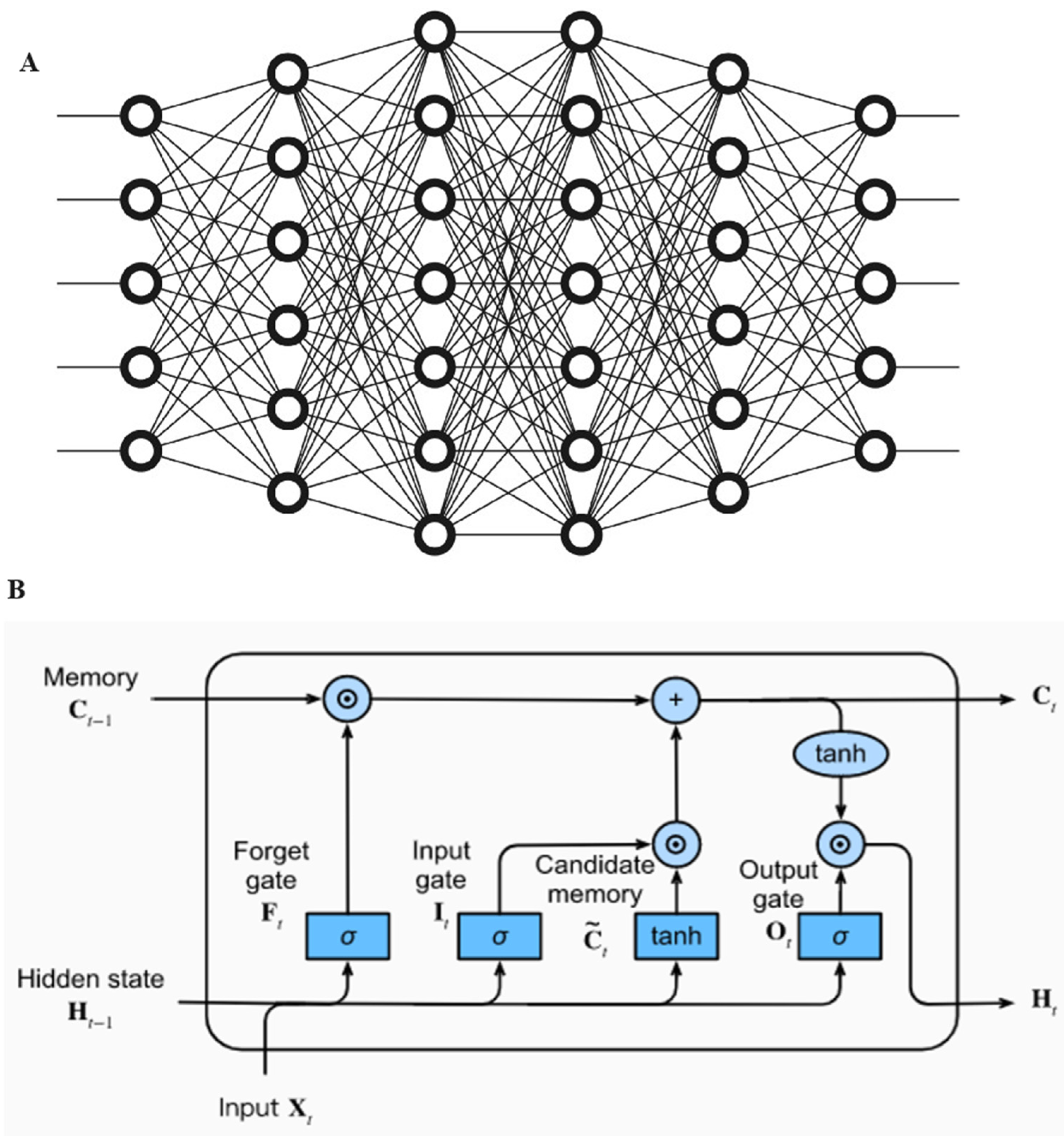
5.1. Fully Connected Deep Neural Network

The FCNN is a type of artificial neural network characterized by its acyclic graph structure. It is considered the most basic and straightforward form of a neural network. The FCNN is a crucial component in machine learning, serving as the foundation for various architectures. It has multiple layers of neurons, each incorporating a nonlinear activation function.
A neural network consists of three distinct types of layers: the input layer, the hidden layer, and the output layer. Hidden layers are a set of intermediary layers positioned between the input and output layers in a neural network. These hidden layers are established by adjusting the parameters of the network. In the case of standard rectangular data, it is commonly observed that the utilization of two to five hidden layers is typically adequate. The quantity of nodes included in each layer is contingent upon the quantity of characteristics in the dataset; however, there exists no rigid guideline governing this relationship. The computational load of the model is influenced by the quantity of hidden layers and nodes; hence the objective is to identify the most sparing model that exhibits a satisfactory performance. The output layer generates the intended output or forecast, and its activation is contingent upon the specific modeling methodology employed. In regression problems, it is common for the output layer to consist of a single node that is responsible for generating continuous numeric predictions. Conversely, in binary classification issues, the output layer normally comprises a single node that is utilized to estimate the probability of success. In the case of a multinomial output, the output layer of the neural network consists of a number of nodes that corresponds to the total number of classes being predicted. Overall, layers and nodes play a crucial role in determining the complexity and performance of neural network models.

5.2. Long Short-Term Memory (LSTM) Deep Neural Network

Long short-term memory (LSTM) is a distinct variant of the recurrent neural network (RNN) architecture, which facilitates the utilization of outputs from previous time steps as inputs for the purpose of processing sequential data. One notable distinction between LSTMand a simple RNN (Recurrent Neural Network) lies in the conditioning of the weight on the self-loop. Unlike simple RNNs, LSTM incorporates contextual information to dynamically adjust the weight on the self-loop. The model effectively captures and preserves enduring relationships between sequential input data, such as time series, text, and speech signals. LSTM models employ memory cells and gates to effectively control the flow of information, enabling the selective retention or removal of information as required. LSTM networks consist of three distinct types of gates, namely input, forget, and output gates. The input gate controls the data stream towards the memory cell, and the other gate, the forget gate, controls the extraction of data from the memory cell. Additionally, the output gate is responsible for controlling the transmission of information from the LSTM unit to the output. The construction of these gates involves the utilization of sigmoid functions, and their training is accomplished through a process of backpropagation. The gates in an LSTM model dynamically modify their openness or closure based on the current input and the previous hidden state. This adaptive mechanism enables the model to effectively choose whether to retain or discard information. The cells of a LSTM network are interconnected in a recurrent manner, provided that the input gate permits it. The state unit is equipped with a self-loop that is regulated by the forget gate, while the output gate has the ability to inhibit the output of the LSTM cell. Figure 3 shows a general diagram for the FCNN and LSTM models, while Table 3 lists the structural components of the FCNN and LSTM models used in this study.

6. Performance Evaluation and Metrics

The following is a description of the experimental setup used in this work. Hardware specifications include a 64-bit operating system, x64-based processor, Intel(R) Core (TM) i5-9400T CPU @ 1.80 GHz running at 1.80 GHz, and 8 GB RAM. Kaggle Notebooks (version 5.5.0, Google, Mountain View, CA, USA) is used to enable, explore, and run machine learning code, with a cloud computational environment based on Jupyter (version 4.7.1, NumFOCUS, Austin, TX, USA) that enables reproducible and collaborative analysis. Python (version 3.7, Python Software Foundation, Beaverton, OR, USA) was the main programming language used.
Predicting the SOH of lithium-ion batteries requires the use of four datasets: DS0005, which is designated for training and validation purposes, and DS0006, DS0007, and DS0018, which are utilized for testing. The purpose of the training set is to facilitate the training process of the model, while the validation set is used to fine-tune the model’s parameters. Lastly, the testing set is employed to evaluate the performance of the model. In order to ensure that the model’s prediction is accurate, a number of suitable hyperparameters must be chosen. I used grid search and cross-validation to obtain the optimal parameters for model performance.

6.1. Performance Evaluation Indicators

This work utilizes three error evaluation metrics, namely root mean square error (RMSE), mean absolute error (MAE), and mean absolute percentage error (MAPE). These metrics are employed to quantitatively analyze the accuracy of the proposed state of health (SOH) prediction model and its Quantized Approximators (QA). The definitions of these metrics are provided as follows:
R M S E = 1 N i = 1 N ( y i y ^ i )   2
M A E = 1 N   i = 1 N y i y ^ i  
M A P E = 1 N i = 1 N y i y ^ i y i × 100 %
In this context, yi represents the actual SOH value, while y ^ i represents the expected (estimated) SOH value. In relation to metrics such as RMSE, MAE, and MAPE, the predictive accuracy increases as these indicators approach zero.

6.2. Model Training

In preparation for the model training phase, I split the training dataset into training and testing data. Using the SOH dataset, we evaluated two distinct ML models, one employing an FCNN and the other an LSTM. The model architectures make up Table 4. In the dataset used for training, which was divided into training and validation data, the training data to validation data ratio was 2:1. The simulation was implemented with Kaggle Environment, based on Jupyter and Python 3.7. Each machine learning model evaluation was executed five times in total, and the average value of all the results was used.
Table 4 shows the batch size, the epochs, the time, and the loss functions that emerged from the training process. It is clearly seen that, because of the large size of the LSTM model, its time for convergence is very large when compared to the simple FCNN model.

7. Evaluation Results and Discussion

The efficiency of the suggested methodology in extracting findings was demonstrated by adapting the FCNN and LSTM learning models for training and inference. I compared the original prediction from the trained model, in both forms, the FCNN and the LSTM, with the LUT prediction for different quantization bits and show the results. To compare and demonstrate the difference between the true SOH and its estimated value utilizing the two neural network learning models, SOH estimation was executed for the FCNN and LSTM learning models, as shown in Table 5. The training used B0005 and prediction used B0006, B0007, and B0018 batteries. In Table 5, the batteries were tested without quantization using actual model validation. Figure 4 shows that SOH estimation follows the same pattern as the real SOH, with a little deviation due to training on a different battery than that tested.
Another setup of SOH predictions for the different batteries at different quantization levels was built to illustrate the accuracy of the suggested quantization when estimating the SOH. Table 6 displays the relevant results. RMSE, MAE, and MAPE are used as error evaluation measures. The table shows the SOH predictions from the deep learning models for B0006, B0007, and B0018 batteries with different quantization bits assigned. The SOH prediction without and with quantization for all bits is illustrated in Figure 5. The FCNN and LSTM models were evaluated with b values of 2, 3, 4, 5, 6, 7, and 8 bits.
To supplement the preceding results, a visual comparison between the quantized and real inferences was prepared. Figure 6 illustrates the comparison between the original estimated SOH and its quantized counterparts for 2 bits and 5 bits.
Initially, the evaluation of the training models was conducted without incorporating quantization operations. This approach aims to provide an understanding of the outcomes in their unaltered state, prior to exploring the impact of quantization. The correlation between the estimated and measured SOH values for a B0006 battery is illustrated in Figure 4. This phenomenon is expected to be applicable to all other batteries, despite the lack of empirical evidence, as has been observed. According to the findings presented in Table 3, it is evident that the two training models exhibit significant differences in terms of elapsed training time, although they have identical batch sizes and epochs. The rationale behind this observation stems from the architectural differences between the LSTM and FCNN models. Specifically, the LSTM model possesses a significantly larger building structure, consisting of over 1.14 million parameters that need to be mathematically computed. In contrast, the FCNN model exhibits a much smaller parameter count, totaling only 217.
Table 5 presents the outcomes of the estimation error analysis of the FCNN training model. The model was trained on the B0005 battery and subsequently evaluated on different batteries using actual model validation, without employing quantization. Divergent error estimations were detected across the two training models across different battery types. In the B0006 battery, the root mean square error (RMSE) of the FCNN model exhibited a superior performance compared to the long short-term memory (LSTM) model by a margin of 0.003, equivalent to a relative improvement of 4.6%. In the case of the B0007 battery, the root mean square error (RMSE) exhibited a difference that favored the LSTM model by 0.0097, which corresponds to a 50% improvement. In the case of the B0018 battery, both the FCNN and LSTM models exhibited similar performances, with a slight advantage of 0.0023 (15%) in favor of the FCNN model. The mean absolute error (MAE) metric revealed a significant disparity in performance for the B0007 battery, with an observed value of 0.0067 (37%). In contrast, the remaining batteries had similar scores in this regard. In terms of the MAPE error metric, the B0006 battery exhibited the smallest disparity, with a score of 2.1%, whilst the FCNN model demonstrated the biggest disparity, with a score of 42%.
Next, I will commence the examination of the impact of quantization on the SOH forecasts for various batteries across different quantization levels and analyze its influence on the accuracy of these predictions. Based on the findings presented in Table 6, it is evident that the accuracy of the SOH prediction utilizing quantization approaches diminishes as the number of quantization bits increases, in comparison to the original non-quantized model’s SOH prediction. Figure 7 shows the three error metrics in relation to the number of quantization bits for B0006 batteries tested using FFN and LSTM models to support the quantization level-error relationship. The results demonstrate that even when employing a limited number of quantization bits, the magnitude of the error remains quite small. Notably, the errors tend to become inconsequential after utilizing a quantization of b = 5 bits. Table 6 provides compelling evidence for the identification of distinct patterns. The findings indicate that the variations in the battery types and the training models, FFN or LSTM, are inconsequential, with the primary distinguishing factor being the number of quantization bits.
Table 6 presents data analysis on the B0006 battery test, which is derived from the dataset utilized by the FCNN model and subsequently approximated using the LUT. The initial values of the root mean square error (RMSE), mean absolute error (MAE), and mean absolute percentage error (MAPE) are 0.0195370, 0.0159236, and 0.0190499, respectively, for a value of b equal to 2 bits. The values obtained when b is equal to 8 bits are 0.0003125, 0.0002565, and 0.0003088, respectively. The ratios are 65 X, 61 X, and 61 X, respectively. The LSTM model demonstrates findings consistent with the RMSE, MAE, and MAPE error measurements. At b = 2 bits, the initial values for these measurements are 0.0216045, 0.0185078, and 0.0225291, respectively. At b = 8 bits, the final values for these measurements are 0.0003309, 0.0002835, and 0.0003446, respectively. The ratios are 65 X, 66 X, and 65 X, respectively. An identical computation can be performed for the remaining batteries.
Figure 5 presents the predictions of the SOH without quantization, as well as with quantization for varying bit values, specifically 2, 3, 4, 5, 6, 7, and 8 bits. However, Figure 6 illustrates that the deviation from the initial prediction (before quantization) becomes insignificant when utilizing 5 or more bits. This implies that a minimum of 5 bits is required in order to obtain distinct agreement with the prediction.

8. Conclusions

This article proposes a replacement and an approximation for the neural network model for battery health estimation. Quantizing all battery SOH features and training FCNN and LSTM networks with pre inference creates a unique LUT memory network replacement model. Furthermore, training data and testing data were collected from NASA to train and test the combined models, respectively. The experiment results show that the proposed method is superior when compared to the algorithms and models that it mimics. It was found that its accuracies were slightly affected by this adoption, when compared to the actual inferred SOH estimation without quantization. The prediction accuracy error was improved up 65X when comparing b =2 bits to b = 8 bits. An average b = 3 bits was found to be a good quantization level, which gave RMSE, MAE, and MAPE error accuracies of 0.0098006, 0.0080317, and 0.0096645, respectively. The novel finding of this work was that b = 5 bits will mostly quantize the seven SOH battery prediction features, totaling 35 bits. However, even with b = 3 bits, the results were satisfactory, with a total of 21 bits. This discovery demonstrates that the LUT operation is reasonable with 2 MB of LUT stored in a memory device giving virtually as accurate results as a full inference model.

Funding

Open Access funding and the APC was funded by Qatar National Library (QNL).

Data Availability Statement

Data are contained within the article.

Conflicts of Interest

The author declares no conflict of interest.

References

  1. Whittingham, M.S. Electrical Energy Storage and Intercalation Chemistry. Science 1976, 192, 1126–1127. [Google Scholar] [CrossRef] [PubMed]
  2. Stan, A.-I.; Swierczynski, M.; Stroe, D.-I.; Teodorescu, R.; Andreasen, S.J. Lithium ion battery chemistries from renewable energy storage to automotive and back-up power applications—An overview. In Proceedings of the 2014 International Conference on Optimization of Electrical and Electronic Equipment (OPTIM), Bran, Romania, 22–24 May 2014; pp. 713–720. [Google Scholar] [CrossRef]
  3. Nishi, Y. Lithium ion secondary batteries; past 10 years and the future. J. Power Sources 2001, 100, 101–106. [Google Scholar] [CrossRef]
  4. Huang, S.-C.; Tseng, K.-H.; Liang, J.-W.; Chang, C.-L.; Pecht, M.G. An online soc and soh estimation model for lithium-ion batteries. Energies 2017, 10, 512. [Google Scholar] [CrossRef]
  5. Goodenough, J.B.; Kim, Y. Challenges for rechargeable Li batteries. Chem. Mater. 2010, 22, 587–603. [Google Scholar] [CrossRef]
  6. Nitta, N.; Wu, F.; Lee, J.T.; Yushin, G. Li-Ion Battery Materials: Present and Future. Mater. Today 2015, 18, 252–264. [Google Scholar] [CrossRef]
  7. Dai, H.; Jiang, B.; Hu, X.; Lin, X.; Wei, X.; Pecht, M. Advanced battery management strategies for a sustainable energy future: Multilayer design concepts and research trends. Renew. Sustain. Energy Rev. 2021, 138, 110480. [Google Scholar] [CrossRef]
  8. Lawder, M.T.; Suthar, B.; Northrop, P.W.C.; DE, S.; Hoff, C.M.; Leitermann, O.; Crow, M.L.; Santhanagopalan, S.; Subramanian, V.R. Battery energy storage system (BESS) and battery management system (BMS) for grid-scale applications. Proc. IEEE Inst. Electr. Electron. Eng. 2014, 102, 1014–1030. [Google Scholar] [CrossRef]
  9. Lai, X.; Gao, W.; Zheng, Y.; Ouyang, M.; Li, J.; Han, X.; Zhou, L. A comparative study of global optimization methods for parameter identification of different equivalent circuit models for Li-ion batteries. Electrochimica Acta 2019, 295, 1057–1066. [Google Scholar] [CrossRef]
  10. Wang, Y.; Gao, G.; Li, X.; Chen, Z. A fractional-order model-based state estimation approach for lithium-ion battery and ul-tra-capacitor hybrid power source system considering load trajectory. J. Power Sources 2020, 449, 227543. [Google Scholar] [CrossRef]
  11. Cheng, G.; Wang, X.; He, Y. Remaining useful life and state of health prediction for lithium batteries based on empirical mode decomposition and a long and short memory neural network. Energy 2021, 232, 121022. [Google Scholar] [CrossRef]
  12. Rechkemmer, S.K.; Zang, X.; Zhang, W.; Sawodny, O. Empirical Li-ion aging model derived from single particle model. J. Energy Storage 2019, 21, 773–786. [Google Scholar] [CrossRef]
  13. Li, K.; Wang, Y.; Chen, Z. A comparative study of battery state-of-health estimation based on empirical mode decomposition and neural network. J. Energy Storage 2022, 54, 105333. [Google Scholar] [CrossRef]
  14. Geng, Z.; Wang, S.; Lacey, M.J.; Brandell, D.; Thiringer, T. Bridging physics-based and equivalent circuit models for lithium-ion batteries. Electrochimica Acta 2021, 372, 137829. [Google Scholar] [CrossRef]
  15. Xu, N.; Xie, Y.; Liu, Q.; Yue, F.; Zhao, D. A Data-Driven Approach to State of Health Estimation and Prediction for a Lithium-Ion Battery Pack of Electric Buses Based on Real-World Data. Sensors 2022, 22, 5762. [Google Scholar] [CrossRef]
  16. Alipour, M.; Tavallaey, S.S.; Andersson, A.M.; Brandell, D. Improved Battery Cycle Life Prediction Using a Hybrid Data-Driven Model Incorporating Linear Support Vector Regression and Gaussian. Chemphyschem 2022, 23, e202100829. [Google Scholar] [CrossRef]
  17. Li, X.; Wang, Z.; Yan, J. Prognostic health condition for lithium battery using the partial incremental capacity and Gaussian process regression. J. Power Sources 2019, 421, 56–67. [Google Scholar] [CrossRef]
  18. Li, Y.; Abdel-Monem, M.; Gopalakrishnan, R.; Berecibar, M.; Nanini-Maury, E.; Omar, N.; van den Bossche, P.; Van Mierlo, J. A quick on-line state of health estimation method for Li-ion battery with incremental capacity curves processed by Gaussian filter. J. Power Sources 2018, 373, 40–53. [Google Scholar] [CrossRef]
  19. Xiong, R.; Li, L.; Tian, J. Towards a smarter battery management system: A critical review on battery state of health monitoring methods. J. Power Sources 2018, 405, 18–29. [Google Scholar] [CrossRef]
  20. Hannan, M.A.; Lipu, M.S.H.; Hussain, A.; Mohamed, A. A review of lithium-ion battery state of charge estimation and management system in electric vehicle applications: Challenges and recommendations. Renew. Sustain. Energy Rev. 2017, 78, 834–854. [Google Scholar] [CrossRef]
  21. Waag, W.; Fleischer, C.; Sauer, D.U. Critical review of the methods for monitoring of lithium-ion batteries in electric and hybrid vehicles. J. Power Sources 2014, 258, 321–339. [Google Scholar] [CrossRef]
  22. Han, X.; Ouyang, M.; Lu, L.; Li, J.; Zheng, Y.; Li, Z. A comparative study of commercial lithium ion battery cycle life in electrical vehicle: Aging mechanism identification. J. Power Sources 2014, 251, 38–54. [Google Scholar] [CrossRef]
  23. Gold, L.; Bach, T.; Virsik, W.; Schmitt, A.; Müller, J.; Staab, T.E.; Sextl, G. Probing Lithium-Ion Batteries’ State-of-Charge Using Ultrasonic Transmission—Concept and Laboratory Testing. J. Power Sources 2017, 343, 536–544. [Google Scholar] [CrossRef]
  24. Robinson, J.B.; Owen, R.E.; Kok, M.D.R.; Maier, M.; Majasan, J.; Braglia, M.; Stocker, R.; Amietszajew, T.; Roberts, A.J.; Bhagat, R.; et al. Identifying defects in li-ion cells using ultrasound acoustic measurements. J. Electrochem. Soc. 2020, 167, 120530. [Google Scholar] [CrossRef]
  25. R-Smith, N.A.-Z.; Leitner, M.; Alic, I.; Toth, D.; Kasper, M.; Romio, M.; Surace, Y.; Jahn, M.; Kienberger, F.; Ebner, A.; et al. Assessment of lithium ion battery ageing by combined impedance spectroscopy, functional microscopy and finite element modelling. J. Power Sources 2021, 512, 230459. [Google Scholar] [CrossRef]
  26. Liu, X.; Zhang, L.; Yu, H.; Wang, J.; Li, J.; Yang, K.; Zhao, Y.; Wang, H.; Wu, B.; Brandon, N.P.; et al. Bridging multiscale characterization technologies and digital modeling to evaluate lithium battery full lifecycle. Adv. Energy Mater. 2022, 12, 2200889. [Google Scholar] [CrossRef]
  27. Onori, S.; Spagnol, P.; Marano, V.; Guezennec, Y.; Rizzoni, G. A New Life Estimation Method for Lithium-ion Batteries in Plug-In Hybrid Electric Vehicles Applications. Int. J. Power Electron. 2012, 4, 302–319. [Google Scholar] [CrossRef]
  28. Plett, G.L. Extended Kalman Filtering for Battery Management Systems of LiPB-Based HEV Battery Packs: Part 3. State and Parameter Estimation. J. Power Sources 2004, 134, 277–292. [Google Scholar] [CrossRef]
  29. Goebel, K.; Saha, B.; Saxena, A.; Celaya, J.R.; Christophersen, J.P. Prognostics in Battery Health Management. IEEE Instrum. Meas. Mag. 2008, 11, 33–40. [Google Scholar] [CrossRef]
  30. Wang, D.; Yang, F.; Zhao, Y.; Tsui, K.-L. Battery Remaining Useful Life Prediction at Different Discharge Rates. Microelectron. Reliab. 2017, 78, 212–219. [Google Scholar] [CrossRef]
  31. Li, J.; Landers, R.G.; Park, J. A Comprehensive Single-Particle-Degradation Model for Battery State-of-Health Prediction. J. Power Sources 2020, 456, 227950. [Google Scholar] [CrossRef]
  32. Hu, X.; Jiang, J.; Cao, D.; Egardt, B. Battery Health Prognosis for Electric Vehicles Using Sample Entropy and Sparse Bayesian Predictive Modeling. IEEE Trans. Ind. Electron. 2015, 63, 2645–2656. [Google Scholar] [CrossRef]
  33. Piao, C.; Li, Z.; Lu, S.; Jin, Z.; Cho, C. Analysis of Real-Time Estimation Method Based on Hidden Markov Models for Battery System States of Health. J. Power Electron. 2016, 16, 217–226. [Google Scholar] [CrossRef]
  34. Liu, D.; Pang, J.; Zhou, J.; Peng, Y.; Pecht, M. Prognostics for State of Health Estimation of Lithium-Ion Batteries Based on Combination Gaussian Process Functional Regression. Microelectron. Reliab. 2013, 53, 832–839. [Google Scholar] [CrossRef]
  35. Khumprom, P.; Yodo, N. A Data-Driven Predictive Prognostic Model for Lithium-Ion Batteries Based on a Deep Learning Al-gorithm. Energies 2019, 12, 660. [Google Scholar] [CrossRef]
  36. Xia, Z.; Qahouq, J.A.A. Adaptive and Fast State of Health Estimation Method for Lithium-Ion Batteries Using Online Complex Impedance and Artificial Neural Network. In Proceedings of the 2019 IEEE Applied Power Electronics Conference and Exposition (APEC), Anaheim, CA, USA, 17–21 March 2019; pp. 3361–3365. [Google Scholar]
  37. Eddahech, A.; Briat, O.; Bertrand, N.; Delétage, J.-Y.; Vinassa, J.-M. Behavior and State-of-Health Monitoring of Li-Ion Batteries Using Impedance Spectroscopy and Recurrent Neural Networks. Int. J. Electr. Power Energy Syst. 2012, 42, 487–494. [Google Scholar] [CrossRef]
  38. Shen, S.; Sadoughi, M.; Chen, X.; Hong, M.; Hu, C. A Deep Learning Method for Online Capacity Estimation of Lithium-Ion Batteries. J. Energy Storage 2019, 25, 100817. [Google Scholar] [CrossRef]
  39. Wu, H.; Judd, P.; Zhang, X.; Isaev, M.; Micikevicius, P. Integer quantization for deep learning inference: Principles and empirical evaluation. arXiv 2020, arXiv:2004.09602. [Google Scholar]
  40. Gong, R.; Liu, X.; Jiang, S.; Li, T.; Hu, P.; Lin, J.; Yu, F.; Yan, J. Differentiable Soft Quantization: Bridging Full-Precision and Low-Bit Neural Networks. In Proceedings of the 2019 IEEE/CVF International Conference on Computer Vision (ICCV), Seoul, Republic of Korea, 27–28 October 2019; pp. 4852–4861. [Google Scholar]
  41. Choi, J.; Wang, Z.; Venkataramani, S.; Chuang, P.I.; Srinivasan, V.; Gopalakrishnan, K. Pact: Parameterized clipping activation for quantized neural networks. arXiv 2018, arXiv:1805.06085. [Google Scholar]
  42. Esser, S.K.; McKinstry, J.L.; Bablani, D.; Appuswamy, R.; Modha, D.S. Learned step size quantization. arXiv 2019, arXiv:1902.08153. [Google Scholar]
  43. Yang, Z.; Wang, Y.; Han, K.; Xu, C.; Xu, C.; Tao, D.; Xu, C. Searching for low-bit weights in quantized neural networks. Adv. Neural Inf. Process. Syst. 2020, 33, 4091–4102. [Google Scholar]
  44. Courbariaux, M.; Bengio, Y.; David, J.P. Binaryconnect: Training deep neural networks with binary weights during propagations. Adv. Neural Inf. Process. Syst. 2015, 2, 3123–3131. [Google Scholar]
  45. Zhu, C.; Han, S.; Mao, H.; Dally, W.J. Trained ternary quantization. arXiv 2016, arXiv:1612.01064. [Google Scholar]
  46. Rastegari, M.; Ordonez, V.; Redmon, J.; Farhadi, A. Xnor-net: Imagenet classification using binary convolutional neural networks. In Proceedings of the European Conference on Computer Vision, Amsterdam, The Netherlands, 11–14 October 2016; Springer International Publishing: Cham, Switzerland, 2016; pp. 525–542. [Google Scholar]
  47. Ullrich, K.; Meeds, E.; Welling, M. Soft weight-sharing for neural network compression. arXiv 2017, arXiv:1702.04008. [Google Scholar]
  48. Xu, Y.; Wang, Y.; Zhou, A.; Lin, W.; Xiong, H. Deep neural network compression with single and multiple level quantization. In Proceedings of the AAAI Conference on Artificial Intelligence, New Orleans, LA, USA, 2–3 February 2018; Volume 32. [Google Scholar]
  49. Zhou, A.; Yao, A.; Guo, Y.; Xu, L.; Chen, Y. Incremental network quantization: Towards lossless cnns with low-precision weights. arXiv 2017, arXiv:1702.03044. [Google Scholar]
  50. Miyashita, D.; Lee, E.H.; Murmann, B. Convolutional neural networks using logarithmic data representation. arXiv 2016, arXiv:1603.01025. [Google Scholar]
  51. Blalock, D.; Gonzalez Ortiz, J.J.; Frankle, J.; Guttag, J. What is the state of neural network pruning? Proc. Mach. Learn. Syst. 2020, 2, 129–146. [Google Scholar]
  52. Gou, J.; Yu, B.; Maybank, S.J.; Tao, D. Knowledge distillation: A survey. Int. J. Comput. Vis. 2021, 129, 1789–1819. [Google Scholar] [CrossRef]
  53. Google. TensorFlow: An End-to-End Open Source Machine Learning Platform. 2019. Available online: https://www.tensorflow.org (accessed on 15 November 2023).
  54. MACE. 2020. Available online: https://github.com/XiaoMi/mace (accessed on 15 November 2023).
  55. Microsoft. ONNX Runtime. 2019. Available online: https://github.com/microsoft/ (accessed on 15 November 2023).
  56. Wang, M.; Ding, S.; Cao, T.; Liu, Y.; Xu, F. Asymo: Scalable and efficient deep-learning inference on asymmetric mobile cpus. In Proceedings of the 27th Annual International Conference on Mobile Computing and Networking, New Orleans, Louisiana, 25–29 October 2021; pp. 215–228. [Google Scholar]
  57. Jiang, X.; Wang, H.; Chen, Y.; Wu, Z.; Wang, L.; Zou, B.; Yang, Y.; Cui, Z.; Cai, Y.; Yu, T.; et al. Mnn: A universal and efficient inference engine. Proc. Mach. Learn. Syst. 2020, 2, 1–3. [Google Scholar]
  58. Liang, R.; Cao, T.; Wen, J.; Wang, M.; Wang, Y.; Zou, J.; Liu, Y. Romou: Rapidly generate high-performance tensor kernels for mobile gpus. In Proceedings of the 28th Annual International Conference on Mobile Computing And Networking, Sydney, Australia, 17–21 October 2022; pp. 487–500. [Google Scholar]
  59. Jiao, Y.; Han, L.; Long, X. Hanguang 800 npu–the ultimate ai inference solution for data centers. In Proceedings of the 2020 IEEE Hot Chips 32 Symposium (HCS), Palo Alto, CA, USA, 16–18 August 2020; IEEE Computer Society: Washington, DC, USA, 2020; pp. 1–29. [Google Scholar]
  60. Jouppi, N.P.; Yoon, D.H.; Ashcraft, M.; Gottscho, M.; Jablin, T.B.; Kurian, G.; Laudon, J.; Li, S.; Ma, P.; Ma, X.; et al. Ten lessons from three generations shaped google’s tpuv4i: Industrial product. In Proceedings of the 2021 ACM/IEEE 48th Annual International Symposium on Computer Architecture (ISCA), Virtual, 14–19 June 2021; pp. 1–14. [Google Scholar]
  61. Wechsler, O.; Behar, M.; Daga, B. Spring hill (nnp-i 1000) intel’s data center inference chip. In Proceedings of the 2019 IEEE Hot Chips 31 Symposium (HCS), Cupertino, CA, USA, 18–20 August 2019; IEEE Computer Society: Washington, DC, USA, 2019; pp. 1–12. [Google Scholar]
  62. Saha, B.; Goebel, K. Battery Data Set, NASA Ames Prognostics Data Repository; NASA Ames: Moffett Field, CA, USA, 2007. [Google Scholar]
  63. Ren, L.; Zhao, L.; Hong, S.; Zhao, S.; Wang, H.; Zhang, L. Remaining Useful Life Prediction for Lithium-Ion Battery: A Deep Learning Approach. IEEE Access 2018, 6, 50587–50598. [Google Scholar] [CrossRef]
  64. How, D.N.; Hannan, M.A.; Lipu, M.H.; Ker, P.J. State of charge estimation for lithium-ion batteries using model-based and data-driven methods: A review. IEEE Access 2019, 7, 136116–136136. [Google Scholar] [CrossRef]
  65. Choi, Y.; Ryu, S.; Park, K.; Kim, H. Machine Learning-Based Lithium-Ion Battery Capacity Estimation Exploiting Multi-Channel Charging Profiles. IEEE Access 2019, 7, 75143–75152. [Google Scholar] [CrossRef]
Figure 1. The new algorithm flowchart and features–bit distribution. (A) LUT memory generation, (B) LUT memory model inference and (C) Features distribution for N = 3, bits total = 21 bits.
Wevj 15 00038 g001
Figure 2. Degradation of lithium-ion batteries as a function of cycle count.
Wevj 15 00038 g002
Figure 3. (A) FCNN Neural Network Model and (B) LSTM Neural Network Model.
Wevj 15 00038 g003
Figure 4. Real B0006 battery SOH and its estimated SOH. The model was trained on a B0005 battery.
Wevj 15 00038 g004
Figure 5. The predicted SOH with no quantization and with quantization for bits b = 2, 3, 4, 5, 6, 7, and 8 was tested on (A) FCNN and (B) LSTM models.
Wevj 15 00038 g005
Figure 6. SOH predictions for a B0006 Battery trained on a B0005 battery dataset, the graph shows the original SOH and its 2-bit and 5-bit quantized versions.
Wevj 15 00038 g006
Figure 7. Effect of quantization on SOH prediction error of (A) FFNN and (B) LSTM) models trained on a B006 battery.
Wevj 15 00038 g007
Table 1. Quantization bits distribution per feature and corresponding SQNR level and total memory size needed.
Bits/FeatureValues GivenBits Total
(Address)
SQNR
dB
Memory Size
241412.0416 K
382118.062 M
4162824.08256 M
5323530.1032 G
6644236.124 T
71284942.14-
82565648.16-
Table 2. Boundaries of the measured features for B0005 battery.
CapacityVmImTmILoadVLoadTime (s)
Min1.287452.44567−2.0290923.2148−1.99840.00
Max1.856484.222930.0074941.45021.99844.2383,690,234
Table 3. Training model specifications.
LayersOutput ShapeParameters No.
Model 1
FCNN
Dense(node, 8)217
Dense(node, 8)
Dense(node, 8)
Dense(node, 8)
Dense(node, 1)
Model 2
LSTM
LSTM 1(N, 7, 200)1.124 M
Dropout 1(N, 7, 200)
LSTM 2(7, 200)
Dropout 2(N, 7, 200)
LSTM 3(N, 7, 200)
Dropout 3(N, 7, 200)
LSTM 4(N, 200)
Dropout 4(N, 200)
Dense(N, 1)
Table 4. Training parameters for B0005 battery dataset.
ModelBatch SizeEpochsTime (s)Loss
FCNN25502000.0243
LSTM255074533.1478 × 10−5
Table 5. Estimation error results for FCNN training model when trained on a B0005 battery and tested on others, using actual model validation (testing) without quantization.
BatteryModelRMSEMAEMAPE
B0006FCNN0.0800100.0682200.100970
LSTM0.0762700.0676200.098770
B0007FCNN0.0195100.0180190.021460
LSTM0.0292820.0247100.030434
B0018FCNN0.0156800.0136100.016890
LSTM0.0180210.0163710.020547
Table 6. The FCNN and LSTM training models endured RMSE, MAE, and MAPE errors when trained on the B0005 battery and tested on the B0006, B0007, and B0018 batteries, each with a different set of quantization bits.
BatteryModelQuantization BitsRMSEMAEMAPE (%)
B0006FCNN20.01953700.01592360.0190499
30.00980060.00803170.0096645
40.00468150.00379880.0045664
50.00243010.00200930.0024294
60.00125350.00103790.0012461
70.00061500.00050680.0006144
80.00031250.00025650.0003088
LSTM20.02160450.01850780.0225291
30.01046580.00884770.0107360
40.00500100.00424870.0051737
50.00258850.00222930.0027206
60.00133940.00116200.0014114
70.00066090.00056920.0006974
80.00033090.00028350.0003446
B0007FCNN20.01876140.01626850.0191451
30.01011810.00882820.0103004
40.00500260.00436510.0051114
50.00244980.00211270.0024730
60.00120300.00104810.0012269
70.00063940.00055660.0006533
80.00030600.00025780.0003013
LSTM20.02096330.01819840.0219105
30.01131470.00996920.0119157
40.00563820.00492960.0059140
50.00273860.00238430.0028542
60.00134950.00118260.0014153
70.00072120.00063200.0007581
80.00034320.00029120.0003475
B00018FCNN20.02052890.01599120.0189426
30.00964510.00775520.0092191
40.00507300.00402540.0047780
50.00229660.00175850.0020886
60.00114920.00087540.0010336
70.00064320.00050050.0005950
80.00029540.00022680.0002719
LSTM20.02185540.01892990.0233109
30.01090690.00947920.0116619
40.00574400.00494720.0060704
50.00265910.00222280.0027317
60.00132550.00114110.0014012
70.00071680.00062080.0007612
80.00034310.00029410.0003649
Disclaimer/Publisher’s Note: The statements, opinions and data contained in all publications are solely those of the individual author(s) and contributor(s) and not of MDPI and/or the editor(s). MDPI and/or the editor(s) disclaim responsibility for any injury to people or property resulting from any ideas, methods, instructions or products referred to in the content.

