Aligned Simulation Models for Simulating Africa’s Electric Minibus Taxis

Abstract

Planning for the eventual electrification of transport in sub-Saharan Africa requires accurate simulation of its unique transport systems. The few studies that attempt to model electric minibus taxis—vehicles extensively used in sub-Saharan Africa’s public transport systems—vary greatly in their results. This paper analyses, compares and corrects the only two existing studies that project energy consumption of electric minibus taxis in the region. One of the studies projected an energy consumption of 0.39 kWh/km, while the other projected 0.93 kWh/km. This paper carefully analyses the simulation tools and models and cumulatively applies corrections from the literature and scientific analyses. As a result, the discrepancy between the two simulation tools is eliminated for a given data input and a final energy consumption is estimated in the range of 0.49–0.52 kWh/km, depending on the input data.

1. Introduction

Africa’s main mode of transport, the minibus taxi, is still fully non-electric. Planning for its eventual electrification in the midst of scarce and unreliable electricity supply requires accurate modelling of the mode’s mobility and its consequential electricity demand. The divergent simulation results in the literature are aligned in this paper, which enables accurate planning for electric mobility in the region.

Public transport in Africa consists primarily of informally operated “minibus taxis”, which autonomously manage their schedules, rates and routes according to the perceived demand. These taxis have become the predominant mode of transport in many countries, providing countless jobs and cheap transport to millions of people every day.

Part of the reason that these vehicles have become so popular is that they are available at a low cost, as second-hand imports from developed countries ([1], p. 348). Unfortunately, this has led to the system being fraught with old, under-maintained vehicles, causing serious environmental concerns. One study done in 12 African cities found that the average age of minibus taxis was 15 years [2]. Powered by internal combustion engines, these vehicles contribute substantially to the emission of greenhouse gases and a general decline of air quality in African cities [3]. Within the next 10 years, these vehicles will need to be replaced with more environmentally and economically sustainable alternatives.

One of the major alternative technologies that have come to the fore in recent times are Electric Vehicles (EVs). Unfortunately, while many developed countries have already started to embrace this technology, African countries have been left behind with almost zero EV penetration, as well as complete uncertainty as to whether their fragile grids and unique transport requirements will make EVs feasible in the African context.

Little research effort has been invested in this space, especially with regard to the electrification of minibus taxis. One of the reasons that have hampered this research is the unavailability of data surrounding public transport of these countries. Routes, fleet sizes, timetables, etc., are vastly undocumented, due to the unregulated nature of public transport. Without this data, it is difficult to forecast the feasibility of and strategise the transition to sustainable public transport [3].

However, the picture is changing, as recent studies try to source [4,5] and characterize taxi movement data [6], and develop open source tools to process this data to perform EV evaluations [7,8].

As a result, Abraham et al. [9] found that electric minibus taxis in South Africa would have an energy consumption of approximately 0.93 kWh/km. (They also obtain similar values for studies conducted using their simulator in other African cities, see Booysen et al. [10], Rix et al. [11].) This led to a total energy consumption of 215 kWh/day. This was concerningly high, as it meant that taxis would either need a large battery or charge multiple times during the day, making taxi electrification quite infeasible in South Africa. After these studies, Hull et al. [12] conducted a study to validate the Abraham et al. result. The result that they obtained was 0.39 kWh/km, significantly lower than that found by Abraham et al..

Although the data landscape is in a poor state, such a large discrepancy is rather unexpected. This study concerns itself with the discrepancy between the two aforementioned studies by analysing the assumptions, methods, models, and data of the two studies.

The key differences between the two studies are as follows:

1.

Abraham et al.’s simulation tool uses an energy-based EV model developed by Kurczveil et al. [13]. In Abraham et al.’s study, their simulation tool was applied to GPS data collected from nine taxis, at 1 sample/minute, over 2 years. These data were collected by Akpa et al. [4]. Although the EV model and the GPS data were not developed/collected by Abraham et al., they are henceforth referred to as Abraham et al.’s EV model and Abraham et al.’s data in order to simplify the discussion;

2.

Hull et al.’s simulation tool uses a custom-built kinetic-based EV model. In Hull et al.’s study, their simulation tool was applied to GPS data collected at 1 sample/second on 62 taxi trips.

The differences between the two studies are further detailed in Section 2.

The discrepancy is analysed in this paper, with the objective of identifying common pitfalls that are overlooked in EV modelling, and to finally contribute the correct energy model and energy consumption per distance value of minibus taxis in Africa.

2. Literature Study (Analysis of Abraham et al. vs. Hull et al.)

As mentioned in the introduction, the study of Abraham et al. projected a minibus taxi energy consumption of 0.93 kWh/km, compared to the 0.39 kWh/km found in Hull et al. This section presents a careful study of Hull et al. and Abraham et al. to identify differences that may have led to the large discrepancy. In addition, it highlights anomalies in both studies which may have introduced other errors.

The differences between the two studies are summarized in

Table 1. Differences between Abraham et al. and Hull et al. studies.

	Abraham et al.	Hull et al.
Data	Per-minute data, 2 years, nine taxis	Per-second data, 62 trips
Routing	Routing required between GPS waypoints. Routes simulated using Lopez et al.’s routing algorithm [14]	No routing required. Routes measured with high-frequency GPS tracking.
EV Model	Peer-reviewed EV model by Kurczveil et al. [13] Rotary inertia modelled. Inertia constant obtained from Fridlund and Wilen [15]; Centrifugal force modelled.	Custom physics-based EV model No rotary inertia modelling; No centrifugal force modelling.

.

2.1. Data Anomalies

The first difference is the characteristics of the data that was used in the studies. As mentioned in Section 1, Hull et al.’s study used high-frequency data, measured at a rate of 1 sample per second, while Abraham et al.’s study used low-frequency data ($\sim 1$ sample per minute). The problem with high-frequency data is that it quickly accumulates to large quantities of data, increasing the cost of the data logging system. The problem with low-frequency data is that the vehicles’ aggressive acceleration profiles and stop–start behaviour are not captured. In addition, since datapoints are sparse, the exact route that the vehicle took has to be inferred. Therefore, low-frequency data needs to be artificially upsampled using a routing/driver model, to synthesize this missing information. Anomalies caused by artificially upsampling the data are discussed in Section 2.2.

Hull et al. limited their study to just 62 trips (24 minutes each) in different driving conditions. On the other hand, Abraham et al. were able to obtain low-frequency data for nine taxis, which were tracked over 2 years. Thus, the Abraham et al. study had a more complete representation of the taxis’ daily and seasonal movement patterns, while the Hull et al. study had a more complete representation of the microscopic acceleration and deceleration patterns and route details.

2.2. Driver/Routing Inconsistencies

Abraham et al.’s simulation tool is designed for low-frequency data. High-frequency data (e.g., 1 Hz data used in Hull et al.) are not common, due to the large storage or high bandwidth that would be required. However high-frequency data, which describe the vehicle’s acceleration and deceleration as well as route details, are needed to accurately simulate an EV model. Abraham et al.’s simulation tool solves this problem by reading a road network to predict the route a vehicle would have taken to go from one waypoint to the next and using a driver model to drive the taxi along this route to upsample the data. This road network is obtained from OpenStreetMap (OSM) [16].

Similar to this study, Giliomee et al. [17] investigated the reasons for the discrepancy between the two studies which evaluate electric minibus taxis, Hull et al. and Abraham et al. They compared the actual manifestations of the road infrastructure, taxi routes, and driving behaviour to their virtual manifestations in Abraham et al.’s simulation. The discrepancies they identified relate to the process that Abraham et al.’s simulation tool uses to upsample the low-frequency data. They identified nine inconsistencies, which fall into three categories:

•   Road network:

  (a)

  Road elevation data was not included in the ev simulation;

  (b)

  Some roads were missing;

  (c)

  Some road segments had incorrect speed limits;

  (d)

  Stop signs were missing and traffic light sequences were incorrect.

• Waypoints:

  (a)

  The simulated vehicle incorrectly stopped at each waypoint along its route; 

  (b)

  Inaccurate GPS data points caused waypoints to fall in oncoming lanes. This led to the simulated vehicles taking multiple U-turns, greatly lengthening the vehicles’ routes.  

• Virtual driver:

  (a)

  In residential roads, the virtual driver travelled at the official speed limit, whereas the actual driver travelled at significantly lower speeds; 

  (b)

  The virtual driver had an excessively aggressive acceleration profile; 

  (c)

  The virtual driver adhered to 100% of stop signs, whereas the actual driver adhered to only 30% of stop signs.  

Out of the road network inconsistencies, most were upstream issues with the road network data provider, OSM [16]. Aside from inconsistency 1a, the inconsistencies would require excessive manual intervention to correct.

Regarding the two waypoint inconsistencies: Inconsistency 2a caused the vehicle to decelerate and accelerate unnecessarily at each waypoint, rather than simply passing them by. Giliomee et al. [17] point out that this would lead to a higher energy consumption and estimate a theoretical compensation factor of −24% to compensate for the error. Since inconsistency 2b mostly affected the total distance that the simulated vehicle travelled, it only affected the total energy consumption, while this study concerns itself with energy consumption per unit distance.

Regarding the inconsistencies in the virtual driver model: Giliomee et al. [17] provide simple remedies to inconsistencies 3a and 3b. Additionally, they find that the energy consumption impact of inconsistency 3c was less than 0.5%, insignificant enough to ignore.

A detailed analysis and description of these inconsistencies can be found in Giliomee et al. [17].

2.3. EV Model Inconsistencies

In addition to the differences in data highlighted above, the two studies also used different EV models. The EV model consumes the vehicles’ routes to calculate the energy requirements of the vehicles. Hull et al. developed their own custom EV model. This model had a few differences with respect to Abraham et al.’s EV model. First, Abraham et al. used a third-party EV model by Kurczveil et al. [13], which is bundled with the Simulation of Urban Mobility (SUMO [14]) software. The model is well-tested and scientifically peer-reviewed. The model used by Hull et al. has been peer reviewed at the time of publication. However, it has had significantly less testing and public exposure than the Kurczveil et al. [13] model. Consequently, mathematical errors in the code are found and addressed in this paper (Section 4.4.2). The features of each model are summarized in

Table 2. EV Model comparison.

	Kurczveil et al. [13]	Hull et al. [12]	Koch et al. [18]
Type of model	Energy	Kinetic	Kinetic
Rotational inertia	✓	×	✓
Radial drag	✓	×	×
Model detail	Simple ${}^{\mathit{a}}$	Simple ${}^{\mathit{a}}$	Detailed ${}^{\mathit{b}}$
Power and torque limiting	×	×	✓
Backward/forward modelling ${}^{\mathit{c}}$	Backward	Backward	Backward
Invalid state reporting ${}^{\mathit{d}}$	×	×	✓

${}^{\mathit{a}}$ Constant recuperation/propulsion efficiency factors. ${}^{\mathit{b}}$ Gear ratio, transmission efficiency factor, 2D motor loss function and battery’s internal resistance are all used to dynamically calculate the propulsion/recuperation efficiency. ${}^{\mathit{c}}$ Backward modelling means that the energy calculations are done after the vehicle’s dynamics have already been established. The EV model does not influence the vehicle’s dynamics, and thus invalid situations can occur. Forward modelling means that the energy calculations are done in conjunction with the vehicle’s dynamics calculations, allowing for EV limitations to be considered. ${}^{\mathit{d}}$ Models with invalid state reporting are able to report states where the mobility profile contains accelerations that are impossible to be satisfied with the given EV model parameters.

. New versions of SUMO also include a detailed EV model by Koch et al. [18], which could be a more accurate drop-in replacement for the Kurczveil et al. [13] model used in Abraham et al.’s simulation tool. That model is therefore included in the summary table as well.

Table 2 shows that Hull et al.’s model does not take into account radial drag and rotational inertia. These parameters may have a significant impact on the vehicles’ energy usage. For example, radial drag accounted for 6% of the energy consumption of buses in Netherlands [19].

The table also shows that Koch et al. [18] do not use simple propulsion/recuperation factors to determine the drivetrain efficiency, allowing for a more detailed setup of the EV model.

Model Parameters

The EV model parameters used in Hull et al. are different from those used in Abraham et al. The model parameters of each study are shown in

Table 3. EV model parameters.

	Abraham et al.	Hull et al.
Mass [kg]	2900	3900
Roll drag coefficient	0.01	0.02
Air drag coefficient	0.35	0.36
Front surface area [${\mathrm{m}}^2$]	4	4
Radial drag coefficient	0.5	-
Internal moment of inertia [$\mathrm{kg}·{\mathrm{m}}^2$ ]	0.01	-
Constant power intake [W]	100	100
Recuperation efficiency	0.5	0.65
Propulsion efficiency	0.8	0.9

. For a fair comparison, the model parameters must be equalized.

Table 3 omits the internal moment of inertia and radial drag coefficient for Hull et al.’s study. This is because the model does not implement these two aspects in the energy model, as mentioned in Section 2.3. In addition, Abraham et al.’s internal moment of inertia is on a significantly lower order of magnitude than other values found in the literature. For example, Koch et al. [18] find a value of 12 $\mathrm{kg}·{\mathrm{m}}^2$ for the BMW i3.

3. Method

The approach taken in this study was to replicate the methods of Abraham et al. and Hull et al., iteratively correcting the anomalies identified in Section 2, as well as other anomalies that were found during the process. As described in Section 2, the anomalies fall under three main categories: data anomalies, driver/routing inconsistencies and EV modelling inconsistencies.

Before correcting anomalies, the studies of Abraham et al. and Hull et al. were first replicated using the latest versions of their simulation tools. After this, the various were fixed, as described in the following sections.

3.1. Data Anomalies

As mentioned in Section 2.1, the two studies used different data sources. It was of interest to see whether using one dataset instead of the other would yield a different result. This was done by running the Abraham et al. data in Hull et al.’s simulation tool and comparing this to Hull et al.’s original result. Likewise, the downsampled Hull et al. data was run in Abraham et al.’s simulation tool and compared that to the original Abraham et al. result.

3.2. Routing Inconsistencies

The first thing to do was to identify which inconsistencies listed in Section 2.2 were worth addressing.

Inconsistencies 1b, 1d, 2b and 3c all had negligible effect on energy consumption according to Giliomee et al. [17], meaning that they could be safely ignored.

The inconsistencies left to be addressed were 1a, 1c, 2a, 3a and 3b. Each of these inconsistencies was addressed as follows, and the simulation was re-evaluated.

As described by Giliomee et al. [17], inconsistency 1a would be resolved by overlaying the OSM road network with elevation data gathered from NASA [20]. This functionality was implemented and merged into Abraham et al.’s simulation tool.

Inconsistency 1c could not be addressed, as it was an upstream issue with OSM, and would require excessive manual intervention to fix. According to Giliomee et al. [17], this issue increases the energy consumption by 11%. The sensitivity analysis of Section 4.6 checks this value, and implications are discussed in the conclusions section.

Inconsistency 2a stated that the vehicle tended to stop at each waypoint encountered in the routes. According to Giliomee et al.’s theoretical approximation, this should reduce the energy consumption by approximately 24% [17]. The validity of their approximation was tested by removing all stops from all the simulation routes, such that the vehicle would pass each waypoint without stopping. This showed that the impact of this inconsistency was much less than anticipated, as shown in Section 4.3. Nevertheless, the issue was fixed by addressing a logical error in the stop detection algorithm (See commit 81caab5 of Abraham et al.’s simulation tool [7]).

Inconsistency 3a was fixed by manually reducing speed limits in the road network. Finally, inconsistency 3b was resolved by changing the driver model’s acceleration and deceleration parameters to the ones given by Giliomee et al. [17].

3.3. EV Modelling Inconsistencies

This study also corrected the inconsistencies in Abraham et al. and Hull et al., which were due to their EV models. These inconsistencies are described in Section 2.3. The two main inconsistencies that are shown in the literature study are:

• The two studies had slightly different model parameters, and the effect of these differences need to be quantified;
• Hull et al. did not implement rotational inertia and radial drag, which may have a significant impact on the vehicles’ energy usage.

After these inconsistencies were fixed, additional analyses and experimentation were needed in order to identify any other sources of error.

3.3.1. Model Parameters and Rotational Inertia

The model parameters, which are different between the two studies, can be seen in Table 3. The model parameters were unified by selecting Hull et al.’s values, and re-simulating Abraham et al.’s study.

Hull et al.’s model parameters were backed up by peer-reviewed sources, whereas Abraham et al.’s parameters were based on SUMO’s default values and Fridlund and Wilen [15]’s bachelor’s thesis. Therefore, Hull et al.’s parameters were deemed more credible.

Rotational inertia and radial drag were suppressed in Abraham et al.’s simulation tool, since they were not implemented in Hull et al.’s simulation tool. The difference caused by suppressing these two parameters was given special focus in the investigation, since the energy consumption results were particularly sensitive to changes in it.

3.3.2. Implementation of Rotary Inertia and Radial Drag

As mentioned above, the Hull et al. model does not implement rotational inertia and radial drag. Since it was found that this is a significant part of the EV modelling process, this study contributes implementations of both these components to Hull et al.’s EV model. These components are implemented in a similar way to that of Kurczveil et al. [13].

The energy lost by the rotary inertia is governed by the formula:

$$\Delta E_{rot}=\frac{I\times \omega }{2}=\frac{I\times v^2}{2\times r_{wheel}^2}$$

(1)

where I is the internal moment of inertia and $r_{wheel}$ is the radius of the vehicle’s wheel.

The energy lost by radial drag is governed by the formula:

$$\Delta E_{rad}=c_{rad}\times \frac{m\times v^2}{r_{curve}}\times \Delta s$$

(2)

where $c_{rad}$ is the radial drag coefficient and $r_{curve}$ is the radius of the turning curve. This radius is calculated using the formula $r_{curve}=\Delta s/\Delta \theta$, where $\Delta \theta$ is the change in the vehicle’s heading angle.

Both these components were added to Hull et al.’s EV model. Thereafter, the effect of the rotary inertia and radial drag constants on the model results were tested.

This revealed that rotary inertia did not affect the energy usage by much. Initially, it was thought that this was caused by an incorrectly selected internal moment of inertia. The value used by Abraham et al. was 0.01 $\mathrm{kg}·{\mathrm{m}}^2$, several orders of magnitude lower than other values found in the literature, such as the 12 $\mathrm{kg}·{\mathrm{m}}^2$ used by Koch et al. [18].

In their code repository [21], Koch et al. suggest a rotary inertia of 16 $\mathrm{kg}·{\mathrm{m}}^2$ for SUV vehicles. Since a value specifically for minibuses could not be found, this value was selected.

This value was roughly validated as follows. The inertia of each wheel was calculated using the equation $I=\frac{1}{2}m{r}^2$, where m is the mass of the wheel and tyre, and r is the outer radius of the tire. For a Toyota Quantum (the prevalent minibus taxi in South Africa), these were $m=23$ kg and $r=345$ mm. This resulted in a rotational inertia of 1.37 $\mathrm{kg}·{\mathrm{m}}^2$. Multiplying this over the four wheels yielded 5.5 $\mathrm{kg}·{\mathrm{m}}^2$. This is a third of the selected value of 16 $\mathrm{kg}·{\mathrm{m}}^2$, leaving two-thirds to account for the gearbox, motor, differential, and other rotating components of the vehicle.

3.3.3. Experimentation to Identify Further Inconsistencies

Section 4.4 shows that there was a residual error after making the above corrections. Therefore, additional experimentation was needed in order to find the source of this residual error. This was done by running both simulations in parallel, stepping through the code line by line and comparing the outputs of all intermediate calculations.

As shown in Section 4.4.2, a significant mathematical error was found. The explanation of the error and the corresponding results are presented in that section.

4. Results

The original energy consumption estimates by Abraham et al. [9] and Hull et al. [12] were 0.93 kWh/km and 0.39 kWh/km, respectively. This section shows how these two values converged when the anomalies mentioned previously were resolved. The original results are compared to the final converged results in

Table 4. Energy consumption [kWh/km] before and after applying the various changes proposed in this paper.

	Abraham Data		Hull Data (Downsampled)		Hull Data (Original)
	Abraham Simulator	Hull Simulator	Abraham Simulator	Hull Simulator	Hull Simulator
Replicated original results	0.88 ${}^{\mathit{a}}$	0.42	0.88	0.45	0.39
Final result	0.50	0.50	0.52	0.52	0.49

${}^{\mathit{a}}$Section 4.1 explains why this is slightly different to the original 0.93 kWh/km reported by Abraham et al.

and Figure 1.

4.1. Replicating Original Results

The two simulations were repeated with the exact same configurations given in Abraham et al. [9] and Hull et al. [12]. Although Hull et al.’s 0.39 kWh was replicated successfully, repeating Abraham et al.’s simulation resulted in a consumption of 0.88 kWh/km. Inspecting the repository’s history revealed two bug fixes that caused this change. Originally, when the results were generated in Abraham et al. [9], power and speed values were cast as integer datatypes, in order to make the software more memory efficient. However, this caused the fractional part of each value to be lost. This led to a large error in the energy and distance values, since they were calculated by integrating speed and power with respect to time. This issue was fixed by version 1.6 of Abraham et al.’s simulation tool (commits b9f1c6e and e50a84e).

4.2. Data Anomalies

The effect of using different types of data was investigated using the approach described in Section 3.1. The results are shown below.

Applying the Hull et al. data to the Abraham et al. model yielded a consumption of 0.88 kWh/km, exactly the same result as that obtained using the Abraham et al. data. Note that, in order for the data to be compatible with Abraham et al.’s simulation tool, the data had to be downsampled from 1 Hz to 1/60 Hz. This was done by selecting a sample every minute and discarding intermediate samples. After this, the data was again upsampled, using the routing algorithm of Abraham et al.’s simulation tool. In order to compare the Hull et al. and Abraham et al. simulation tools with the same input data, the downsampled Hull et al. data was fed into the Hull et al. simulation tool to obtain a result of 0.45 kWh/km.

Applying the upsampled Abraham et al. data to the Hull et al. model yielded an energy consumption of 0.42 kWh/km. (Note: Giliomee et al. [17] report a value of 0.44 kWh/km. This slight discrepancy is due to the software patch described in Section 4.1.) In order for the data to be compatible with Hull et al.’s simulation tool, the data had to be upsampled from 1/60 Hz to 1 Hz. This was done by running the data through the routing algorithm of Abraham et al.’s simulation tool, and feeding the resulting 1 Hz data into Hull et al.’s simulation tool. The difference between the two results is 0.03 kWh/km. This could be because of the different driving patterns inherent in the two datasets.

From the above two analyses, it is quite clear that the inconsistency lies more with the simulators than with the data. For consistency and simplicity of the discussion, the downsampled Hull et al. data will be used to generate the results in the remainder of this paper.

4.3. Routing Inconsistencies

This section describes the results that were found by implementing the fixes described in Section 3.2.

After implementing elevation (inconsistency 1a), Abraham et al.’s result remained at 0.88 kWh/km. However, Hull et al.’s result increased to 0.47 kWh. A slight increase was expected, since the excess energy required to climb a hill would not be completely recuperated when braking downhill. After implementing the corrected acceleration parameters (inconsistency 3b), both results dropped drastically. Abraham et al.’s result dropped to 0.67 kWh/km, while Hull et al.’s dropped to 0.44 kWh/km.

To fix inconsistency 3a, traffic was emulated by reducing the taxis’ maximum speed to 25 km/h on residential roads (as suggested by Giliomee et al. [17]). This lowered Abraham et al.’s result to 0.63 kWh/km and Hull et al.’s result to 0.43 kWh/km.

The effect of inconsistency 2a was tested using the approach described in Section 3.2. The result of those experiments showed that this issue affected the result very marginally. Removing the waypoint stops increased Abraham et al.’s result slightly, to 0.67 kWh/km, and decreased Hull et al.’s result to 0.42 kWh/km. Although Giliomee et al. [17] approximated an offset of −24%, this experiment indicated an offset of −2% to +6% (depending on the simulator used).

By analysing the stop detection algorithm, it was found to be labelling datapoints as stops when the vehicle was actually moving at those points. (The reason for the bug was that the downsampled Hull et al. data was downsampled at fixed intervals of 1 min per sample. The stop detection algorithm was designed for dynamically sampled data such as that of Abraham et al.) Correcting the stop-detection algorithm led to an energy consumption of of 0.62 kWh/km and 0.42 kWh/km for the Abraham et al. and Hull et al. simulation tools, respectively.

4.4. EV Modelling Inconsistencies

4.4.1. Investigation of Model Parameters

The scenario was re-simulated using Hull et al.’s model parameters. This again lowered Abraham et al.’s result significantly, from 0.62 to 0.49 kWh/km, much closer to Hull’s result of 0.42 kWh/km.

The two model parameters that were not implemented in Hull’s simulator were rotary inertia and radial drag. Therefore, these two model parameters were set to zero, as shown in Table 3.

These two parameters were implemented in Hull et al.’s simulation tool, using the same modelling techniques as Kurczveil et al. [13]. Each of these model parameters were then restored to Abraham et al.’s values to quantify their effect. It was found that rotary inertia affected the result minimally, decreasing Abraham et al.’s result by 0.02 kWh/km, while not affecting Hull et al.’s result.

By doing more careful modelling of the rotary components of the vehicle, a more accurate rotary inertia of 16 $\mathrm{kg}·{\mathrm{m}}^2$ was found, as described in Section 3.3.2. This time, Abraham et al.’s results decreased by 0.01 kWh/km instead of 0.02 kWh/km, while Hull et al.’s result again stayed the same.

Similarly, Abraham et al.’s radial drag value was also restored. Unlike rotary inertia, this impacted the results significantly. Abraham et al.’s result increased to 0.76 kWh/km, while Hull et al.’s result increased to 0.70 kWh/km.

According to Fridlund and Wilen [15], it is extremely difficult to accurately calculate the radial drag coefficient. They, therefore, recommend using SUMO’s default value. In their initial study [9], Abraham et al. had incorrectly assumed that 0.5 was the default radial drag coefficient in SUMO. Upon closer inspection of SUMO’s documentation, the correct default was only 0.1. Re-simulating the scenario with the correct value resulted in a more modest increase to 0.52 kWh/km in the Abraham et al. case and 0.47 kWh/km in the Hull et al. case.

4.4.2. Mathematical Model Correction

After making all the model parameters equal, there was still a discrepancy between the two EV models. To identify the source of this discrepancy, both both simulations were run in parallel, stepping through the code line by line and comparing the outputs of all intermediate calculations.

The Abraham et al. model calculated the propulsive energy as follows:

$$E_{prop}=\Delta E_{kin}+\Delta E_{pot}+E_{aero\_drag}+E_{roll\_drag}+E_{rad\_drag}$$

(3)

On the other hand, the Hull et al. model calculated the propulsive energy as follows:

$$E_{prop}=F_{prop}\times \Delta x$$

(4)

where $\Delta x$ is the distance travelled.

$F_{prop}$ was calculated by assuming that the difference between the measured velocity and the expected velocity (caused by drag forces) is caused by $F_{prop}$. Therefore:

$$\begin{array}{cc}\hfill F_{prop}\left[n\right]& =m\times a_{prop}\hfill \end{array}$$

(5)

$$\begin{array}{cc}\hfill & =m\times \frac{v\left[n\right]-v_{exp}\left[n\right]}{\Delta t\left[n\right]}\hfill \end{array}$$

(6)

where $v_{exp}\left[n\right]$ is the expected velocity due to external forces (gravity, aerodynamic drag, and rolling resistance) at timestep n, $\Delta t\left[n\right]=t\left[n\right]-t[n-1]$, and m is the vehicle’s mass.

The problem with this approach is the transition from Equation (5) to Equation (6). Both $v\left[n\right]$ and $v_{exp}\left[n\right]$ are both at timestep n, which goes against the definition of acceleration ($a\left[n\right]=\left(v\right[n]-v[n-1\left]\right)/\left(t\right[n]-t[n-1\left]\right)$).

The correct form of Equation (6) has a complex derivation, so it is omitted here, but it can be proven wrong by expanding Equation (3) as follows:

From Equation (3):

$$\begin{array}{c}\hfill E_{prop}=\frac{1}{2}m\left({v\left[n\right]}^2-{v[n-1]}^2\right)-mg\Delta h-F_{roll\_drag}\Delta x-F_{aero\_drag}\Delta x\end{array}$$

(7)

If substituting Equation (6) into Equation (4) does not yield Equation (7), it will prove that Equation (6) is incorrect. Substituting Equation (6) into Equation (4):

$$E_{prop}=\frac{m\Delta x}{\Delta t}\times \left(v\left[n\right]-v_{exp}\left[n\right]\right)$$

(8)

According to Hull et al.’s definition of $v_{exp}$:

$$\begin{array}{cc}\hfill v_{exp}& =v[n-1]+\sum \left(a_{drag}\times \Delta t\right)\hfill \\ \hfill & =\begin{array}{c}\hfill v[n-1]+\frac{F_{roll\_drag}}{m}\Delta t+\frac{F_{aero\_drag}}{m}\Delta t+\frac{mg\Delta h/\Delta x}{m}\Delta t\end{array}\hfill \end{array}$$

(9)

Substituting Equation (9) into Equation (8):

$$\begin{array}{cc}\hfill E_{prop}& =\begin{array}{c}\hfill \frac{m\Delta x}{\Delta t}\times \left(v\left[n\right]-v[n-1]-\frac{F_{roll\_drag}}{m}\Delta t-\frac{F_{aero\_drag}}{m}\Delta t-\frac{mg\Delta h/\Delta x}{m}\Delta t\right)\end{array}\hfill \\ \hfill & =\begin{array}{c}\hfill \frac{\left(v\right[n]-v[n-1\left]\right)m\Delta x}{\Delta t}-F_{roll\_drag}\Delta x-F_{aero\_drag}\Delta x-\frac{m^{2}g\Delta h}{m}\end{array}\hfill \\ \hfill & =\begin{array}{c}\hfill {\left(v\left[n\right]-v[n-1]\right)}^{2}m-F_{roll\_drag}\Delta x-F_{aero\_drag}\Delta x-mg\Delta h\end{array}\hfill \end{array}$$

(10)

Comparing Equations (10) and (7) shows that the kinetic energy term is incorrect in Equation (10). That is,

$${\left(v\left[n\right]-v[n-1]\right)}^2\ne \frac{1}{2}\left({v\left[n\right]}^2-{v[n-1]}^2\right)$$

Thus, it is proven that the assumption taken in Hull’s model was incorrect. The Hull et al. simulation tool was thus adapted to follow the same modelling approach as Abraham et al..

This resulted in a value of 0.52 kWh/km, the same value found by the Abraham et al. model at the end of Section 4.4. Thus, the two models produced the same result of 0.52 kWh/km.

4.5. Final Result

After all of the fixes above were completed, the energy consumption output by both simulators agreed for the Hull et al. downsampled data. Repeating the simulations with the Abraham et al. data yielded energy consumption of 0.50 kWh/km in both simulators. Repeating the simulation using the original high frequency Hull et al. data yielded an energy consumption of 0.49 kWh/km.

4.6. Sensitivity Analysis

To aid with future assessments of electric paratransit, this section performs a sensitivity analysis of some of the inconsistencies in Section 2.2 and parameters in Table 3. This parameter sensitivity analysis shows how much each parameter affects the result (compared to the correct result), and is summarized in

Table 5. Sensitivity analysis: simulator parameters, performed with the Hull et al. data, downsampled and interpolated with 1 Hz SUMO simulator (Section 2.2).

Aspect (Inconsistency Number)	Consumption If Uncorrected
	[kWh/km] (% Error)
Driver acceleration (3b)	0.60 ($+15\%$)
Elevation (1a)	0.53 ($+2\%$)
Waypoint progression (2a)	0.53 ($+2\%$)
Residential driver speed profile (3a)	0.51 ($-3\%$)
Legal speed limits (1c)	0.50 ($-3\%$)

and

Table 6. Sensitivity analysis—electro-kinetic model parameters, performed with the Hull et al. data, downsampled and interpolated with 1 Hz SUMO simulator (Section 3.3).

Parameter	Working point	Consumption if Not Implemented [kWh/km] (% Error)	Consumption with Parameter Variation
			Parameter $\Delta =-\mathbf{10}\%$ [kWh/km] (%$\Delta$)	Parameter $\Delta =-10\%$ [kWh/km] (%$\Delta$)
Mass [kg]	3900	–	0.48 ($-8\%$)	0.56 (+8%)
Roll drag coefficient	0.02	–	0.50 ($-4\%$)	0.54 ($+4\%$)
Air drag coefficient	0.36	0.44 ($-15\%$)	0.51 ($-2\%$)	0.53 (+2%)
Front surface area [${\mathrm{m}}^2$]	4	–	0.51 ($-2\%$)	0.53 (+2%)
Radial drag coefficient	0.1	0.45 ($-13\%$)	0.51 ($-1\%$)	0.53 (+1%)
Internal moment of inertia [$\mathrm{kg}·{\mathrm{m}}^2$ ]	16	0.53 (0%)	0.52 (0%)	0.52 (0%)
Constant power offtake [W]	100	0.52 (0%)	0.52 (0%)	0.52 (0%)
Recuperation efficiency	0.65	0.68 (+32%)	0.54 ($+3\%$)	0.50 ($-3\%$)
Propulsion efficiency	0.90	0.45 ($-13\%$)	0.60 (+15%)	0.46 ($-12\%$)

.

Table 5 shows that the driver acceleration parameters are the most important to get correct, out of the various simulator parameters. If left uncorrected, a 15% error in the result is introduced.

The last row of the table shows the impact of inconsistency 1c. As discussed in Section 3.2, Giliomee et al. [17] found that the issue had an 11% impact. This was concerning, since this was the only issue with a non-zero impact issue that was left unresolved in this study. Thankfully, with respect to the corrected model, this issue only has a −3% impact factor. Therefore, the issue can safely be ignored.

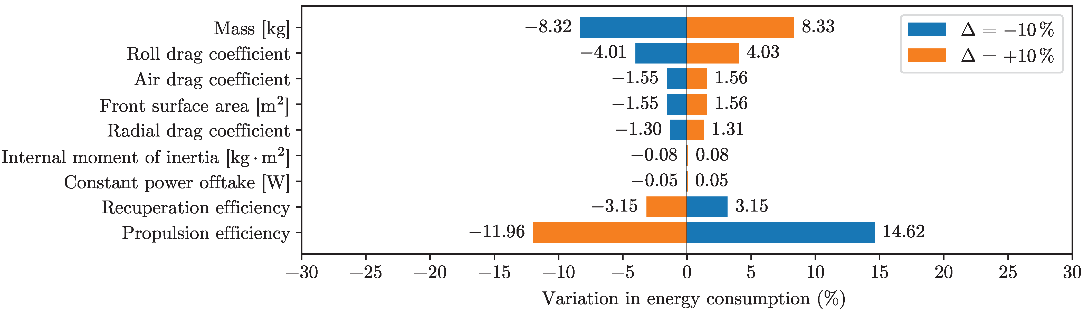
Table 6 shows the sensitivity of various parameters of the EV model. It shows that propulsion efficiency has the highest sensitivity. This means that it is essential to select this value as accurately as possible. Finding these parameter values vary in difficulty. According to Fridlund and Wilen [15], Table 5.4, the following parameters are hard to find (in increasing order of difficulty): roll drag coefficient, power offtake, recuperation efficiency, propulsion efficiency, radial drag coefficient and internal moment of inertia.

The results of the sensitivity analysis are presented graphically in Figure 2. It shows that, out of all the parameters, roll drag coefficient, propulsion and recuperation efficiency are the only ones with a significant sensitivity. Fortunately, although the roll drag coefficient is difficult to find accurately, it is easy to approximate [15], Table 5.4. Given that the sensitivity is 4%, an approximation should suffice. Therefore, recuperation and propulsion efficiencies are the parameters that need to be obtained most carefully.

This study implements two parameters in the Hull model, which were previously missing. One was the internal moment of inertia. Table 6 shows that the implementation of this parameter had a negligible impact on energy consumption. On the other hand, radial drag had a large impact. When not implemented, it affected the result by −13%. This value roughly corresponds with the −6% observed by Beckers et al. [19] for urban buses in the Netherlands. One can assume that radial drag losses would be higher for minibus taxis, since they do a lot of cornering due to the highly tortuous (winding) nature of their routes, as observed by Ndibatya and Booysen [6].

4.7. Application of Results

In Hull et al. [12], the authors apply their model (which had an average consumption rate of 0.39 kWh/km) to estimate the range that would be achieved given various battery sizes. These values are re-computed using the updated consumption rate of 0.49 kWh/km to obtain

Table 7. Updated range estimations for Hull et al.’s study, using the updated consumption rate of 0.49 kWh/km.

Battery Size [kWh]	Range [km]
	Updated Consumption Rate	Original Consumption Rate
50	87	109
75	130	163
100	173	218

. A total of 85% of the battery capacity is assumed to be available.

Additionally, some of the key results of Abraham et al. [9] are also revised in

Table 8. Updated key metrics of Abraham et al. [9].

Metric	Updated Value	Original Value
Average daily energy consumption per taxi	115 kWh	215 kWh
Charging power required to meet average energy consumption if a charger is available at all major stops	18 kW	32 kW
Total photovoltaic area required to self-generate average daily energy demand without battery storage	170 ${\mathrm{m}}^2$	320 ${\mathrm{m}}^2$
Additional demand on daily national energy generation, if all taxis in South Africa are electrified	5.5%	10%

, using the updated consumption rates.

5. Conclusions

The minibus taxi is one of the most widely used forms of public transport in Africa. However, despite it prevalence, surprisingly little research has been invested to prepare the industry for emerging EV technologies. The only two studies which have evaluated EV taxis (namely Abraham et al. and Hull et al.) have conflicting results. This study evaluated the two aforementioned studies in order to find the reasons for the discrepancy and obtain a more accurate result.

In order to do this, the data, mobility model, and EV model aspects of the two studies were compared and analysed as follows. Regarding the data, the primary difference between the two studies was the data resolution. Hull et al.’s data was captured at 1 Hz, while Abraham et al.’s data was captured at $\sim 1/60$ Hz. Abraham et al.’s simulator uses a mobility model to interpolate the routes and acceleration profiles between its sparse datapoints. Suggestions by Giliomee et al. are incorporated to more accurately model the specific mobility patterns of minibus taxis. Lastly, the study analysed the model parameters and the mathematics behind the two EV models to finally reconcile their outputs. A final output between 0.49–0.52 kWh/km was observed, depending on the input data. A sensitivity analysis of the above discrepancies revealed the following. For the data aspect, downsampling the Hull et al. data increased the consumption from 0.49 to 0.52 kWh/km, an error of 6%. For the mobility model aspect, the error caused by selecting wrong acceleration parameters led to an error of 15%. For the EV model aspect, the most sensitive model parameters were mass, roll-drag, recuperation efficiency and propulsion efficiency, with sensitivities between 3% and 15% in the output per 10% change in the model parameter. However, the difficulty in measuring the latter two parameters make them the most critical. Furthermore, for the EV model aspect, a mathematical error in Hull et al.’s model was found which caused an error of 10% in the result.

These results have implications for future electric taxi evaluations. Firstly, it is clear that high frequency data is needed to ensure that the aggressive acceleration profiles and tortuous routes are captured. If data logging limitations do not allow for high frequency data collection, a mobility model such as that of Abraham et al. may be used to synthesize the missing data. However, the high sensitivity of the acceleration model parameters underscores the importance of accurately modelling the unique mobility patterns of electric taxis. Despite our best efforts to do this, a 6% error was still observed. Although this was less significant than the sensitivity of parameters in the mobility and EV models, it reinforces Hull et al.’s statement that the frequency of data collection has a notable impact on energy consumption calculations. The EV model analysis showed that the propulsion and recuperation efficiency parameters need to be selected carefully. This issue could be avoided by using a more detailed EV model, which calculates these efficiencies by modelling the motor, power electronics and drivetrain components. Because of this study’s holistic approach, some of the sensitivity values calculated by Giliomee et al. were invalidated, due to corrections made in other aspects of the electric taxi model. For example, the issue of incorrect legal speed limits was found to have a significantly less impact than initially predicted. Giliomee et al. predicted a sensitivity of +11%, but the updated model had only a $-3\%$ error.

The novelty of this study is that it contributes corrections to two existing EV minibus taxi simulation tools, and contributes a more accurate energy consumption per distance value for minibus taxis in Africa. Some further work can be envisioned as a result of this research. Firstly, the 6% discrepancy between the results of the artificially downsampled Hull et al. data versus the original 1 Hz Hull et al. data needs to be examined. Secondly, a detailed EV model needs to be incorporated into the simulation tools in order to reduce the uncertainty of estimating the propulsion and recuperation efficiency parameters. Thirdly, work needs to be done to correct anomalies that affect the total energy consumption of the vehicle. Finally, an empirical validation is envisaged, using a physical electric taxi to validate the result of 0.49–0.52 kWh/km and calibrate the model parameters.

References

- Cervigni, R.; Rogers, J.A.; Dvorak, I. Assessing Low-Carbon Development in Nigeria: An Analysis of Four Sectors; World Bank: Washington, DC, USA, 2013. [Google Scholar]
- Kumar, A.M.; Foster, V.; Barrett, F. Stuck in Traffic: Urban Transport in Africa; Technical Report; AICD: Washington, DC, USA, 2008. [Google Scholar]
- Collett, K.A.; Hirmer, S.A. Data needed to decarbonize paratransit in Sub-Saharan Africa. Nat. Sustain. 2021, 4, 562–564. [Google Scholar] [CrossRef]
- Akpa, N.E.E.; Booysen, M.; Sinclair, M. Publicly Available Annotated Dataset of Tracked Taxis. 2016. [Dataset]. Available online: https://gitlab.com/eputs/data/fcd-stellenbosch (accessed on 1 March 2023).
- DigitalTransport4Africa. Data. 2022. [Dataset]. Available online: https://digitaltransport4africa.org/ (accessed on 1 March 2023).
- Ndibatya, I.; Booysen, M.J. Characterizing the movement patterns of minibus taxis in Kampala’s paratransit system. J. Transp. Geogr. 2021, 92, 103001. [Google Scholar] [CrossRef]
- Abraham, C.J.; Rix, A.; Booysen, M.J. Electric-Vehicle Fleet Simulator (ev-fleet-sim). 2022. [Software]. Available online: https://ev-fleet-sim.online (accessed on 18 August 2023).
- Hull, C.; Giliomee, J.; Collett, K.A.; McCulloch, M.; Booysen, M. Bumpy Ride. 2022. [Software]. Available online: https://github.com/ChullEPG/Bumpy-Ride (accessed on 18 August 2023).
- Abraham, C.; Rix, A.; Ndibatya, I.; Booysen, M. Ray of hope for sub-Saharan Africa’s paratransit: Solar charging of urban electric minibus taxis in South Africa. Energy Sustain. Dev. 2021, 64, 118–127. [Google Scholar] [CrossRef]
- Booysen, M.; Abraham, C.; Rix, A.; Ndibatya, I. Walking on sunshine: Pairing electric vehicles with solar energy for sustainable informal public transport in Uganda. Energy Res. Soc. Sci. 2022, 85, 102403–102413. [Google Scholar] [CrossRef]
- Rix, A.; Abraham, C.; Booysen, M. Why taxi tracking trumps tracking passengers with apps in planning for the electrification of Africa’s paratransit. iScience 2022, 25, 104943. [Google Scholar] [CrossRef] [PubMed]
- Hull, C.; Giliomee, J.; Collett, K.A.; McCulloch, M.D.; Booysen, M. High fidelity estimates of paratransit energy consumption from per second GPS tracking data. Transp. Res. Part Transp. Environ. 2023, 118, 103695. [Google Scholar] [CrossRef]
- Kurczveil, T.; López, P.Á.; Schnieder, E. Implementation of an Energy Model and a Charging Infrastructure in SUMO. In Proceedings of the Simulation of Urban Mobility; Behrisch, M., Krajzewicz, D., Weber, M., Eds.; Springer: Berlin/Heidelberg, Germany, 2014; pp. 33–43. [Google Scholar]
- Lopez, P.A.; Behrisch, M.; Bieker-Walz, L.; Erdmann, J.; Flötteröd, Y.P.; Hilbrich, R.; Lücken, L.; Rummel, J.; Wagner, P.; Wießner, E. Microscopic Traffic Simulation using SUMO. In Proceedings of the 2019 IEEE Intelligent Transportation Systems Conference (ITSC), Maui, HI, USA, 27–30 October 2019; pp. 2575–2582. [Google Scholar]
- Fridlund, J.; Wilen, O. Parameter Guidelines for Electric Vehicle Route Planning. 2020. Available online: https://www.diva-portal.org/smash/get/diva2:1460796/FULLTEXT01.pdf (accessed on 1 March 2023).
- OpenStreetMap Contributors. Planet Dump. 2017. Available online: https://planet.osm.org (accessed on 1 March 2023).
- Giliomee, J.; Hull, C.; Collett, K.A.; McCulloch, M.; Booysen, M. Simulating Mobility to Plan for Electric Minibus Taxis in Sub-Saharan Africa’s Paratransit. Transp. Res. Part D 2023, 118, 103728. [Google Scholar] [CrossRef]
- Koch, L.; Buse, D.S.; Wegener, M.; Schoenberg, S.; Badalian, K.; Dressler, F.; Andert, J. Accurate physics-based modeling of electric vehicle energy consumption in the SUMO traffic microsimulator. In Proceedings of the 2021 IEEE International Intelligent Transportation Systems Conference (ITSC), Indianapolis, IN, USA, 19–22 September 2021; pp. 1650–1657, Preprint. Available online: https://www2.tkn.tu-berlin.de/bib/koch2021accurate/koch2021accurate.pdf (accessed on 1 March 2023). [CrossRef]
- Beckers, C.J.; Besselink, I.J.; Nijmeijer, H. Assessing the impact of cornering losses on the energy consumption of electric city buses. Transp. Res. Part Transp. Environ. 2020, 86, 102360. [Google Scholar] [CrossRef]
- National Aeronautics and Space Administration, Shuttle Radar Topography Mission, 2015. [Dataset] Data Obtained from USGS Earth Explorer. Available online: https://earthexplorer.usgs.gov/ (accessed on 1 March 2023).
- Koch, L.; Buse, D.S.; Wegener, M.; Schoenberg, S.; Badalian, K.; Dressler, F.; Andert, J. SUV.xml. 2021. [Datafile]. Available online: https://github.com/mechatronics-RWTH/sumo/blob/ev_powertrain_device/data/VehicleParams/SUV.xml (accessed on 18 August 2023).