State of Health Prediction for Lithium-Ion Batteries through Curve Compression and CatBoost

Abstract

This study proposes a novel approach for predicting the State of Health (SoH) and Remaining Useful Life (RUL) of lithium-ion batteries. The low accuracy of SoH and RUL is due to the challenges of establishing effective feature engineering for battery attributes. To address this issue, a SoH and RUL prediction model based on curve compression and CatBoost is proposed. Firstly, an improved threshold selection method based on curvature analysis is introduced to enhance the compression performance of battery attributes under different cycles. Secondly, to ensure that the extracted feature sequences have the same length, spline interpolation and local anomaly factor detection techniques are utilized to fill or eliminate feature points for feature length normalization. Finally, a dynamic time regularization algorithm is applied to calculate the shortest distance between the feature sequence and the original curve to determine the optimal feature length for input into the CatBoost prediction model. The experimental results demonstrate that the proposed approach outperforms other prediction models in the research object dataset, achieving $R^2$ values higher than 0.98 and MSE values around 1 × 10⁻⁵. The proposed approach also achieves better prediction results in the validation object dataset, indicating its strong generalization capability. Additionally, the proposed model shows significant robustness by accurately predicting SoH and RUL under noisy environmental conditions. Overall, the proposed model shows significant potential to accurately predict SoH and RUL by efficiently addressing the challenges associated with feature engineering for battery attributes, reducing the impact of background noise on prediction results, and exhibiting strong robustness.

1. Introduction

Lithium-ion batteries are widely used in various fields due to their high energy density, long cycle life, and high safety performance. Lithium-ion batteries have become essential in many applications, ranging from portable electronic devices to the rapid development of new energy electric vehicles, aerospace, and other fields [1,2,3,4,5]. However, they are also prone to performance degradation and uncertain failure. As the energy supply and core component of the entire power system, battery failure can lead to a decline in overall system performance, safety accidents, and economic losses. The performance degradation process of lithium-ion batteries is complex and involves various physical and chemical changes. In actual operation, the battery is subject to different charging and discharging modes, current magnitude, environmental pressure and temperature, as well as the battery manufacturing process itself, all of which interact with each other, resulting in non-deterministic and non-linear characteristics that make it challenging to accurately predict the battery degradation performance and ensure the stability and safety of lithium-ion batteries in different operating environments. As a result, stability and safety remain major challenges in the development of lithium-ion batteries [6,7,8,9,10]. To address this issue, it is essential to develop accurate methods for estimating the State of Health (SoH) and Remaining Useful Life (RUL) of the battery.

In recent times, the growing sophistication of artificial intelligence, machine learning, and data mining methodologies has led to increased interest in data-driven approaches for predicting SoH. Researchers have utilized advanced machine learning techniques to establish the correlation between battery SoH and Remaining Useful Life, and the relevant features to achieve accurate prediction [11,12,13,14,15,16]. In their study, Yue et al. [17] proposed a fresh health factor for lithium-ion batteries that relies on the amplitude of the instantaneous voltage drop in the initial segment of discharge under a constant-current discharge condition. To minimize noise, they employed multi-order Bezier curves to reconstruct the new health factor data and devised an empirical degradation model for the battery predicated on the number of cycles. Zhou et al. [18] also proposed a data-driven model for predicting the State of Health (SoH) of batteries in the face of noise. Their approach was based on the Temporal Convolutional Network (TCN), which consists of multilayer causal convolution and can encode the sequence of sampling points on the battery charging curve. They found that the proposed TCN-based SoH estimation model achieved high accuracy and demonstrated good adaptability to different types of batteries. Additionally, Ezemobi E et al. [19] analyzed a method to enhance the generalization of SoH estimation using the Parallel Layer Extreme Learning Machine (PL-ELM) algorithm to extend the application of a single SoH estimation model to a large number of cells of the same type. Furthermore, in response to the problems of many complicated model parameters and time-consuming existing SoH estimation methods, Feng et al. [20] propose to characterize the battery capacity degradation using directly measurable battery constant current charging time and discharge voltage sample entropy as HIs (Health Indicators). The hierarchical extreme learning machine (HELM) model is introduced to establish the SoH online estimation framework, and the two newly constructed HIs are used as inputs to train the HELM battery degradation model offline to achieve SoH online estimation.

In data-driven battery SoH prediction, it is necessary to extract typical features from the capacity degradation data of the battery and establish a mapping relationship between these features and the health state. In previous research, Liu et al. [21] used the ratio of current capacity to the nominal capacity of lithium-ion batteries as HI. However, this approach can ignore useful information during training and degrade generalization performance. Che et al. [22] proposed an efficient health factor extraction method for battery cells based on partial charge and discharge data while considering a feature generation strategy for battery pack capacity decay and inconsistency and using dual time scale filtering and a battery pack equivalent circuit model to broaden the application scope of the feature extraction method. Finally, a Gaussian process-based regression algorithm framework is used to improve the estimation accuracy and reliability, and the method improves the accuracy of battery system health state estimation as well as its adaptability in widely used scenarios. In their study, Liu et al. [23] utilized an improved Douglas–Peucker compression algorithm to compress the discharge voltage curve of the battery dataset from the University of Maryland and build an XGBoost model. However, their approach extracted fewer features, and the generalization ability of the model with fewer features in the actual prediction needs to be demonstrated. On the other hand, Zhang et al. [24] propose a method for estimating the health state of lithium-ion batteries based on the incremental energy method and Bi-directional Gated Recurrent Network (BiGRU) Dropout. Firstly, the maximum peak height in the incremental energy curve is extracted as the new health factor of the battery SoH. The mapping relationship between the health factor and SoH is derived from the BiGRU network built by the flip-flop layer and the gated recurrent network layer, and its experimental results show that the method can estimate the battery SoH quickly and accurately under different charging multiplier conditions.

The technique of curve compression, also known as curve simplification or point set extraction thinning, is a useful data compression technique that reduces the amount of data by removing some data points while ensuring sufficient accuracy. Curve compression is commonly used in mapping, road network analysis, robot path planning, and various other fields. The utilization of curve compression algorithms can significantly reduce the data volume while still maintaining the main shape features and path direction information of the original curve without affecting the importance of the original data. Among curve compression algorithms, the perpendicular distance threshold algorithm and the Douglas–Peucker algorithm are the most widely used. The Douglas–Peucker algorithm requires more computational resources and many iterations. On the other hand, the perpendicular distance threshold algorithm calculates the distance from each point to the line segment, resulting in lower computational complexity and a significant advantage when dealing with large amounts of data. Additionally, the parameters of the perpendicular distance threshold algorithm can be adjusted according to specific needs and have better retention of some key core curve features.

In the field of data-driven SoH and RUL prediction for lithium-ion batteries, neural networks, Unsupervised learning, and ensemble learning algorithms are commonly used. Unsupervised learning can be used to detect abnormal conditions in battery operation, such as excessive temperature, abnormal voltage, capacity drop, etc. By modeling the normal behavior of the battery, the state of the battery can be monitored in real time, and potential problems can be detected in time so that early action can be taken to avoid battery failure [25]. Ensemble learning algorithms combine multiple learners and have better learning performance. Gradient Boosting Decision Tree (GBDT) is a powerful ensemble learning algorithm that reduces total error and enhances robustness by minimizing bias. It has been successfully applied in various fields, such as transportation, finance, medicine, and lithium battery lifetime prediction. CatBoost, a machine learning library founded by Yandex, is based on the GBDT framework and was introduced in 2017. Compared to other GBDT algorithms like XGBoost and LightGBM, CatBoost offers several improvements. It addresses gradient bias during iteration through the use of the ordering principle, ordering enhancement algorithms, and a greedy strategy to reduce overfitting, optimize model speed, and enhance the model’s robustness and accuracy. Moreover, CatBoost uses a weighted random negative sampling method and symmetric tree splitting to increase the generalization ability of the tree model. It has exhibited excellent performance in transformer fault diagnosis and has become a popular choice when dealing with large-scale datasets with high dimensionality and multiple discrete variables [26].

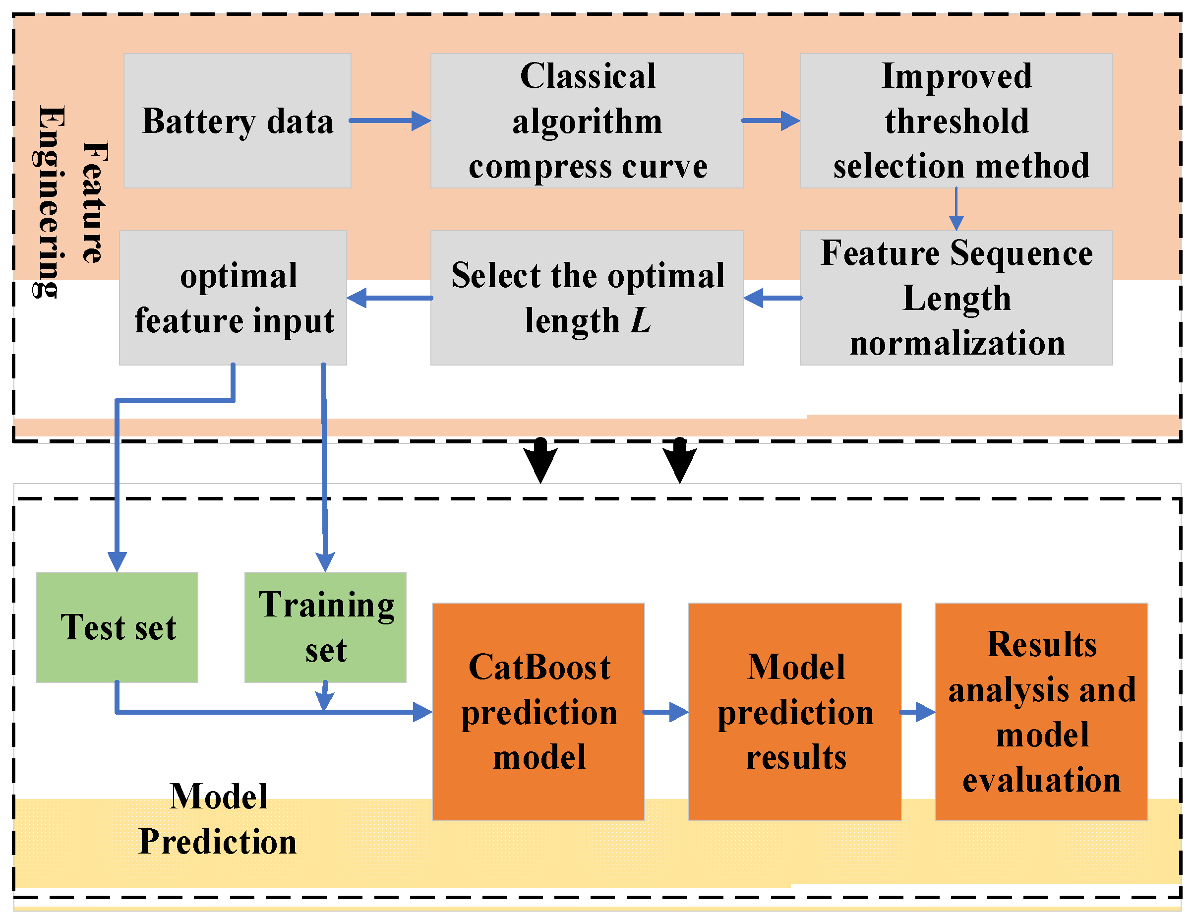
To address the issue of low accuracy in predicting SoH and RUL of lithium-ion batteries due to the difficulty of feature engineering, this study proposes a SoH and RUL prediction model based on curve compression and CatBoost. Firstly, a threshold selection method that integrates curvature analysis for improvement is proposed to improve the unsatisfactory compression results of the classic perpendicular distance threshold algorithm when applied to compressing the original curve. Second, cubic spline interpolation and the Local Outlier Factor (LOF) method are used to fill or eliminate the feature to ensure that the extracted feature sequences are of the same length and can be easily input into the prediction model. Then, the dynamic time regularization algorithm is used to calculate the shortest distance between the feature sequence and the original curve and use it as the basis for judgment to determine the optimal length, and the feature is used as the input to the CatBoost prediction model for SoH estimation and RUL prediction of lithium-ion batteries. Finally, to verify the superiority of the established feature engineering and the model used in this study, experiments such as comparison of the effects of different prediction models, model generalization validation, and model robustness validation are conducted to demonstrate the different dimensions.

2. Algorithm Introduction

2.1. Curve Compression Algorithm

The essence of curve compression is to reduce the amount of information while maintaining the key characteristics of the curve. The main idea is to select a subset $x$ from the dataset $X$ that constitutes the curve that can represent the curve’s characteristics within an allowable error and minimize data redundancy. The perpendicular distance threshold algorithm is one of the most widely used curve compression algorithms, which essentially extracts the characteristic points of the curve using point-to-line distance. This method has the advantages of simplicity, high applicability, and comprehensive feature information extraction.

2.1.1. Douglas–Peucker Algorithm

The Douglas–Peucker algorithm is a classical curve compression algorithm that follows the steps below:

Step 1: Connect an imaginary line between the first and last points of the curve to be compressed and calculate the distances from the remaining points to the line.

Step 2: Select the point with the largest distance and compare it with the threshold value. If it is greater than the threshold value, then the point with the largest distance from the line is kept. Otherwise, all the points between the two end points of the line are discarded.

Step 3: Based on the retained points, the known curve is divided into two parts, and the operations of steps 1 and 2 are repeated. The point with the largest distance is still selected and compared with the threshold value. The points are selected and discarded in turn until there are no more points to be discarded. Finally, the coordinates of the curve points that meet the given accuracy limit are obtained. Specific details are shown in the Figure 1.

2.1.2. Perpendicular Distance Threshold Algorithm

The perpendicular distance threshold algorithm shares the same principle as the Douglas–Peucker algorithm, but it does not consider the entire curve from a global perspective. Instead, it selects and removes redundant points starting from the first point. That is, starting from the first point, the perpendicular distance between the second point and the line connecting the first and second points is calculated. If this distance is greater than the given threshold, the second point is retained and used as a new starting point, and the distance between the third point and the line connecting the second and third points is calculated. Otherwise, the second point is removed, and the distance between the third point and the line between the 1st and 4th points is calculated. This process is repeated until the last point of the curve is reached. Specific details are shown in the Figure 2.

2.2. CatBoost Algorithm Principle

The CatBoost algorithm is a unique boosting algorithm that utilizes improved gradient-boosting decision trees. It distinguishes itself by employing a ranking boosting technique, which helps overcome gradient and prediction bias problems and minimizes overfitting. Furthermore, CatBoost uses a symmetric tree-based learner to enhance the generalization ability and prediction speed of the model, achieving both high accuracy and efficient training. With its remarkable robustness and high accuracy, CatBoost outperforms other algorithms despite having fewer parameters.

Figure 3 illustrates the fundamental principle of the boosting algorithm. Initially, a subset of data is selected, and initial weights are assigned to the data points in this subset. Next, a weak learner is trained on this subset, and the prediction errors of the weak learner are evaluated. The weights of the training samples with high error rates are increased, allowing the weak learner to focus on these samples in the next round of learning. This iterative process is repeated, gradually enhancing the performance of the learner. Finally, larger weights are assigned to the weak learners that exhibit a higher level of learning accuracy, and multiple weak learners are combined and weighted to produce a strong learner.

2.2.1. Gradient Boosting Algorithm (GBDT)

The GBDT algorithm is a widely used ensemble learning algorithm that employs Classification and Regression Trees (CART) as the base learner. It has a basic structure resembling that of a decision tree forest, and its learning method is gradient boosting [27]. The major principle of the GBDT algorithm involves constructing a weak learner that mitigates the shortcomings within the current model by continuously iterating towards the steepest slope direction to minimize the loss. This approach enables the model to achieve superior classification and prediction results for nonlinear data.

Step 1. Initialize the weak learner. For the input training dataset:

$$T=\{(x_1,y_1),(x_2,y_2),\dots ,(x_n,y_n)\}$$

(1)

where $x_i\in X\subseteq R^n$, $y_i\in Y\subseteq R^n$. The initial model is a tree with only one root node:

$$f_0(x)=arg{\min }_c{\displaystyle \sum _{i=1}^{N}L(y_i,c)}$$

(2)

where $x$ denotes the model input variable; $y_i$ denotes the output variable; $c$ denotes the constant value that minimizes the loss function; $L$ is the model loss function; and $N$ is the number of variables.

Step 2. For $m=1,2,\dots ,M$, calculate each input sample $i=1,2,\dots ,N$,

$$r_{mi}=-{[\frac{-\partial L(y_i,f(x_i))}{\partial f(x_i)}]}_{f(x)=f_{m-1}(x)}$$

(3)

where $r_{mi}$ denotes the generalized residual corresponding to the $m$th tree.

Step 3. The residuals obtained in the previous step are used as the new true values of the samples, and the data $\left(x_i,x_{mi}\right)$ are used as the training data for the next tree to obtain a new regression tree whose corresponding leaf node region of the $m$th tree is $R_{mj}$, $j=1,2,\dots ,J$. Where $J$ denotes the number of leaf nodes in the regression tree. For the leaf region $j=1,2,\dots ,J$, the calculation is performed,

$$C_{mj}=arg {\min }_c{\displaystyle \sum _{x_i\in R_{mj}}L(y_i,f_{m-1}(x_i)+c)}$$

(4)

where, $C_{mj}$ denotes the best prediction value that minimizes the loss function of the region $R_{mj}$.

Step 4. Obtain the best-fit regression tree for this round of iteration $f_m(x)$,

$$f_m(x)={\displaystyle \sum _{j=1}^j{C}_{mj}I(x\in R_{mj})}$$

(5)

where, $I$ denotes the output regression tree.

Step 5. Updating the Strong Learner.

$$F_m(x)=f_{m-1}(x)+{\displaystyle \sum _{j=1}^J{C}_{mj}I(x\in R_{mj})}$$

(6)

where, $F_m(x)$ denotes the updated regression tree model.

Step 6. Obtain the strong learner expression:

$$F_M(x)={\displaystyle \sum _{m=1}^M{\displaystyle \sum _{j=1}^J{C}_{mj}I(x\in R_{mj})}}$$

(7)

where $F_M(x)$ is the regression lift tree.

2.2.2. CatBoost Algorithm

Similar to other typical gradient-boosting algorithms, CatBoost also fits the gradient of the current model by building a new tree. However, CatBoost addresses the problem of overfitting, which is a common issue in standard boosting algorithms, by implementing some enhancements to the classical gradient boosting approach. The algorithmic steps involve the following:

Let $D$ be the training set:

$$D=(x_i,y_i)$$

(8)

where $n$ is the number of sample groups $(i=1,2,\dots ,n)$, each group of samples is $x_i=(x_i^1,x_i^2,\dots ,x_i^m)$, $x_{\mathrm{i}}^{\mathrm{m}}$ is the eigenvector of the $m$th sample of the $i$th group, and $y_i$ is the target value of the $i$th.

The feature transformation values $X_i^k$ of the CatBoost model are:

$$X_i^k=\frac{{\displaystyle \sum _{j=1}^n\phi (x_j^k=x_i^k)y_j+\alpha P}}{{\displaystyle \sum _{j=1}^n\phi (x_j^k=x_i^k)+\alpha }}$$

(9)

where $\phi$ is the indicator function, $P$ is the prior value; $\alpha$ is the prior weight. They reduce the noise problem for categories with a low frequency of occurrence.

In CatBoost, the traditional gradient estimation method is replaced by Ordered Boosting, which involves training a separate model for each sample in the training set to obtain an unbiased gradient estimation. To achieve this, during training, a corresponding model is obtained by training the base learner using all other samples in the training set except for the current sample. By repeatedly training the base learner and using gradient estimate values of sample data, the final model is obtained, thereby improving the model’s generalization ability. This approach ensures an accurate prediction for individual samples and enhances the overall performance of the model.

3. Lithium-Ion Battery SoH Prediction Process

To predict the SoH of lithium-ion batteries, this study proposes a model based on curve compression and feature engineering using CatBoost. The prediction process of this model is shown in Figure 4.

The SoH prediction process in this research is divided into two parts: feature engineering and model prediction, as shown in Figure 4. Firstly, the classical perpendicular distance threshold algorithm is used to compress the collected battery signal, and an improved threshold selection method is proposed by integrating curvature analysis to address the issue of unsatisfactory compression results caused by traditional threshold selection. Secondly, to ensure that the extracted feature sequences have the same length and are easy to input into the prediction model, the feature length is achieved by filling or eliminating feature points using the third spline interpolation and LOF anomaly detection normalization. Then the dynamic time regularization algorithm is used to calculate the shortest distance between the feature sequence and the original curve, and the optimal length L is determined based on the best similarity between the feature sequence and the original curve. Finally, the training set and the test set are divided, and the CatBoost prediction model is used with the feature input for battery SoH prediction and multidimensional model evaluation.

4. Data Acquisition

4.1. Experimental Protocol

4.1.1. Experimental Setup

To conduct cyclic charge/discharge experiments on an NCM battery, commonly used in electric cars, a battery tester is employed in this study. The battery tester measures voltage, current, power, capacity, and other relevant parameters throughout the experimental process. The experimental setup comprises a middleware (Neware, Shenzhen, China), an alligator clip, a Supervisory Control and Data Acquisition computer (Windows10), and a thermostatic chamber (Ling). The thermostatic chamber serves the purpose of maintaining a stable experimental environment of 15 °C. Figure 5 illustrates the experimental setup used in this study.

The experimental battery is an 18,650 lithium-ion battery, and its detailed parameters are presented in

Table 1. Specific parameters of the experimental battery.

Projects	Specification	Projects		Specification
Housing material	Nickel-plated steel	Charging strategy (CC/CV) Operating temperature	Standard	0.5C_5A × 7.5 h
Nominal capacity	1300 mAh		Fast	1C_5A × 2.5 h
Rated capacity	3.7 V		Charging	0 °C~45 °C 32 °F~113 °F
Charging Voltage (Max)	4.2 V
Discharge cut-off voltage	2.7 V		Discharge	−15 °C~60 °C 5 °F~140 °F
Charging Current (Max)	1 C5
Discharge current (Max)	3 C5		Storage	−20 °C~60 °C −4 °F~113 °F
Internal resistance (Max at 1000 Hz)	≤25 mΩ

.

4.1.2. Experimental Steps

In order to analyze battery aging under different working conditions, this study conducts two different charging/discharging strategy experiments, including constant voltage and constant current charging with constant power discharging and constant voltage with constant current charging and constant current discharging. The experimental process is as follows:

Experiment 1. Constant voltage and constant current charging with constant power discharging:

Step 1:

Charge at a constant current of 1 A until the battery reaches 4.2 V using a battery tester.

Step 2:

Charge at a constant current of 4.2 V until the detection current is less than 200 mA, then stop charging.

Step 3:

Let the battery stand for 10 min.

Step 4:

Discharge at a constant power of 6 W until the battery voltage drops to 2.7 V, then stop discharging.

Step 5:

Leave the battery on for 20 min.

Step 6:

Repeat steps 1–5 for a total of 148 cycles.

Experiment 2. Constant voltage and constant current charging with constant current discharging:

Step 1:

Charge at a constant current of 1.3 A until the battery reaches 4.2 V using a battery tester.

Step 2:

Charge at a constant voltage of 4.2 V until the detected charging current is less than 50 mA, then stop charging.

Step 3:

Let the battery stand for 10 min.

Step 4:

Discharge at a constant current of 3.9 A until the battery voltage drops to 2.7 V, then stop discharging.

Step 5:

Leave the battery on for 20 min.

Step 6:

Repeat steps 1–5 for a total of 148 cycles.

Figure 6 shows the experimental flow for constant voltage and constant current charging with constant current discharging.

As shown in Figure 6, the constant-current followed by the constant-voltage charging method was used in this experiment, which can shorten the charging time and ensure the safety of the experimental battery. The battery was charged at a low rate of 0.5 C (1.3 A) of constant current until it reached 4.2 V and then charged at a constant voltage of 4.2 V until the current dropped to 0.2 A. Discharge was performed using either a constant current discharge of 1.5 C (3.9 A) or a constant power discharge of 6 W to a cut-off voltage of 2.7 V. Finally, a predetermined number of charge/discharge cycles was used as the experimental termination condition to record the experimental data, draw the discharge capacity curve, and analyze it to obtain the constant power discharge curve and constant current discharge curve. These curves were named battery 1 and battery 2, respectively.

In this study, the battery’s SoH is described using its capacity, which is defined as:

$$SoH=1-\frac{C_{init}-C_{batt}}{0.2C_{init}}$$

(10)

where $C_{init}$ denotes the rated capacity, $C_{batt}$ denotes the actual capacity, and $0.2<C_{batt}<C_{init}$.

The Remaining Useful Life (RUL) of a lithium-ion battery refers to the number of cycles between the point of capacity decay and the 80% capacity level. The EOL standard sets the battery failure thresholds for B0005, B0006, and B0007 at 1.38 Ah, 1.38 Ah, and 1.50 Ah, respectively. This means that B0005 requires 128 cycle count points to reach the failure threshold for the first time, B0006 requires 112 cycle count points, and B0007 requires 125 cycle count points. Figure 7 depicts the original State of Health (SoH) curves obtained using varying charging and discharging strategies.

4.2. Introduction to the Dataset

To validate the effectiveness of the proposed algorithm for lithium-ion batteries, this study carries out experiments using two distinct datasets, which are referred to as dataset A and dataset B. Through these experiments, the algorithm’s performance is evaluated and compared with other existing methods, and the results obtained help to determine the algorithm’s suitability for practical battery applications.

Dataset A consists of test data for a lithium-ion battery rated at 2 Ah, collected by the NASA Prediction Center (Prognostics Center of Excellence, PCoE). The data was obtained from three different batteries, namely B0005, B0006, and B0007. The collected data includes voltage readings taken during the battery’s charge and discharge cycles. Charging is performed using a current of 1.5 A until the voltage reaches 4.2 V, after which a constant voltage is applied until the charging current falls below 20 mA. Discharging is performed using a constant current of 2.0 A until the voltage drops to 2.5 V. The battery undergoes this charging and discharging cycle for a total of 168 cycles.

Dataset B contains data obtained from the experimental procedure described in Section 4.1, which includes measurements of voltage, current, and power during the charging, resting, and discharging periods of the battery. This dataset specifically involves 148 cycles of the battery after undergoing processing.

5. Instance Validation

This study focuses on dataset A, which is subjected to curve compression and used as the subject of research. A prediction model is developed to forecast the State of Health (SoH) and Remaining Useful Life (RUL) of each battery group. Dataset B is used as a validation dataset to assess the generalizability of the proposed feature engineering approach. Feature engineering is performed again on dataset B, and a prediction model is constructed to evaluate the performance of the prediction.

5.1. Traditional Threshold Selection Method: Compress Curve

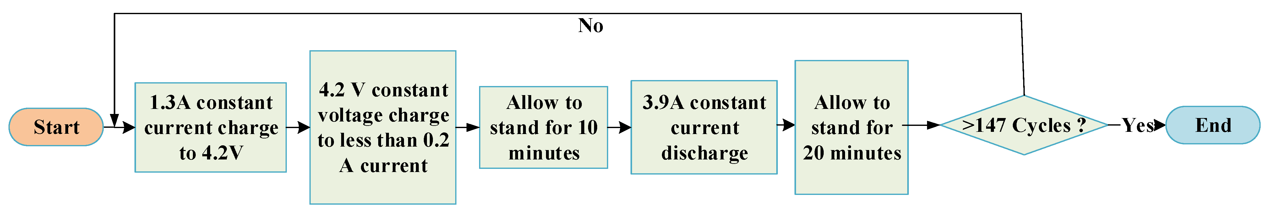
In this study, dataset A is selected for experimentation, which comprises various charging and discharging cycles of lithium-ion batteries. Each cycle is composed of ten different attributes: Voltage measured, Current measured, Temperature measured, Current load, and Voltage load for charging, and Voltage measured, Current measured, Temperature measured, Current load, and Voltage load for discharging. To showcase the experimental process of curve compression and threshold selection, the Voltage measured attribute of battery number five is used as an example.

The discharge experiment conducted on battery number five in dataset A generated the Voltage-measured attribute time-domain decay curves shown in Figure 8.

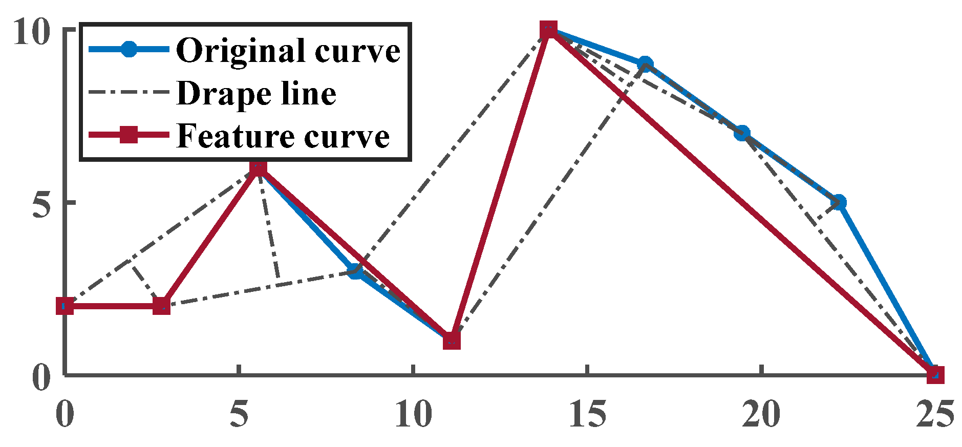
The charge curves of the Voltage-measured attribute in each cycle of the discharge experiment conducted on dataset A are demonstrated in Figure 8. However, when testing and monitoring lithium batteries, different experiments and application scenarios require data collection at different sampling frequencies. Some tests may require a higher sampling frequency to obtain more detailed and accurate data, while others may only require a lower sampling frequency. The inconsistent sampling points in each curve make it challenging to use this attribute directly for battery life prediction, warranting the need for feature extraction. Additionally, the curve shapes under different cycles are similar, with common features such as upper convexity and lower concavity. By capturing curve detail information, the data length can be significantly reduced and the model complexity minimized. The curve compression is performed using the perpendicular distance threshold algorithm for feature point extraction. However, the traditional pendant limit method has limitations in threshold value selection, including (1) uncertainty in threshold value selection, which can lead to inadvertent deletion of feature points, and (2) the selected threshold values are not directly related to the data compression rate, making the number of compression points indeterminate.

To investigate the threshold selection issue of voltage curve compression using the perpendicular distance threshold algorithm, the Voltage measured curves of the 5th and 105th discharge cycles in Figure 8 were selected and analyzed using the classical perpendicular distance threshold algorithm under different threshold conditions. The curve compression results under different thresholds are presented in Figure 9 and Figure 10, respectively. The conventional thresholds consist of the median of the dip ${\epsilon }_1$ and the minimum value of the line from each point on the curve to the first and last end points ${\epsilon }_2$.

The compression results of different curves in Figure 9 and Figure 10 reveal that the feature intervals obtained by the perpendicular distance threshold algorithm differ for different threshold conditions, which significantly impact the compression effect of the final solution. As observed in Figure 9, selecting the median vertical distance threshold ${\epsilon }_1$ retains more points for both curves, resulting in a low data compression rate (i.e., ratio of the compressed curve data points to the original curve points) and high spatial complexity, which does not achieve the intended purpose of reducing feature dimension. On the other hand, selecting the minimum distance ${\epsilon }_2$ as the threshold leads to a high compression rate but a poor fit between the compressed and original real curves. Additionally, curve feature point extraction under different thresholds performed well at curve segments with significant changes in slope but poorly at curve segments with a flat trend, indicating that the traditional threshold selection method does not satisfy the requirements of all points on a given curve.

In summary, the compression results show significant errors under both threshold selections, indicating that excessively large or small thresholds can cause significant measurement errors. It is feasible to adjust the threshold size to adapt to all the Voltage measured curves. The fundamental issue lies in the fact that the threshold judgment criteria of the classical perpendicular distance threshold algorithm cannot adequately capture the deviation of certain curve segments from their corresponding straight lines. Therefore, it is necessary to propose a new threshold judgment criterion that builds on the classical perpendicular distance threshold algorithm to achieve more accurate curve compression.

5.2. Improved Threshold Selection Method Compress Curve

The threshold value in the classical perpendicular distance threshold algorithm cannot effectively capture the linearity of the original curve, leading to different states in the obtained intervals of the original curve. While the linearity of the fitting results can be enhanced by adjusting the threshold, a uniform threshold value cannot be applied to all curves, making it challenging to set the threshold accurately.

Assessing the deviation of the entire curve from the line connecting the first and last points requires considering the curvature of the curve, which can be effectively analyzed using curvature analysis. Conventional curvature analysis evaluates the degree of deviation of discrete data points from the desired curve, where the curvature of a plane curve in two-dimensional plane space is defined as the rotation rate of the tangent direction angle to the arc length at a point on the curve, indicating the extent of curve deviation from the straight line. In this study, curvature is characterized as the deviation of a curve segment from the line connecting the first and last points of a gentle curve segment. Therefore, to calculate the mean curvature at a point $x_0$ on the curve $f$, the reciprocal of the radius of a circle that is tangent to the curve at $x_0$ and two nearby points on the curve is computed as follows:

$$r=\frac{{(1+{(f^{\prime }(x_0))}^2)}^{3/2}}{|f^{\prime \prime }(x_0)|}$$

(11)

where $f^{\prime }(x_0)$ and $f^{\prime \prime }(x_0)$ denote the first and second order derivatives of the curve $f$ at $x_0$, respectively, $f^{\prime \prime }(x_0)\ne 0$, and $r$ denotes the radius of the close circle.

$${\epsilon }_K=\frac{1}{N}{\displaystyle \sum _{i=1}^N\frac{1}{\mathrm{r}}}$$

(12)

In Equation (12), $N$ represents the number of data points of the original curve, and ${\epsilon }_K$ represents the mean curvature of the curve segment.

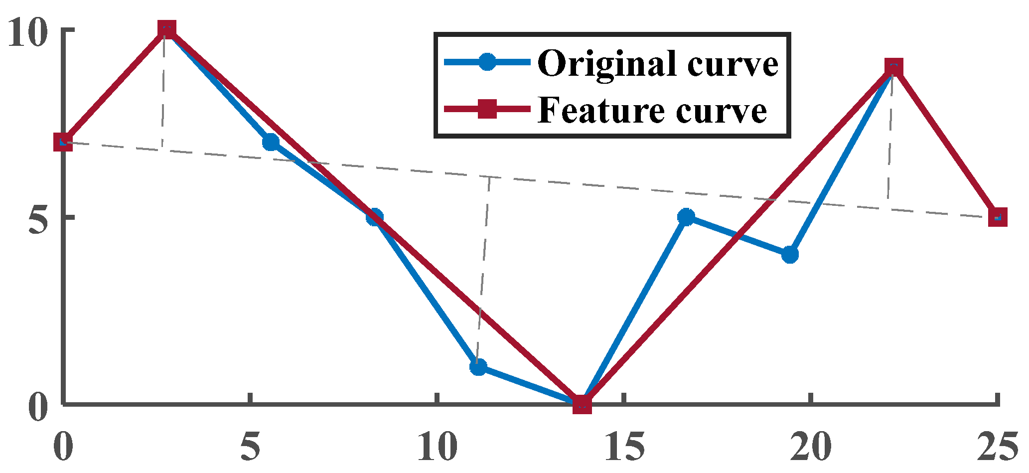
To identify the flat change area in the original curve segment, the derivatives at each point of the curve are computed, and the area with relatively minor changes in the derivatives is selected. Based on this area, the first and last end points of the gentle line segment can be determined. Figure 11 illustrates the first and last end points of the 5th discharge voltage curve’s gentle line segment.

After obtaining the gentle curve segment, the mean curvature of the line connecting each point on the segment to the first and last end points is computed to determine the curvature threshold. The traditional threshold is then replaced with the curvature threshold, and the improved threshold selection method is used in combination with the drape limit algorithm to perform curve compression on the original curve. The compression results for the voltage curve under two different cycles in Figure 8 are illustrated in Figure 12.

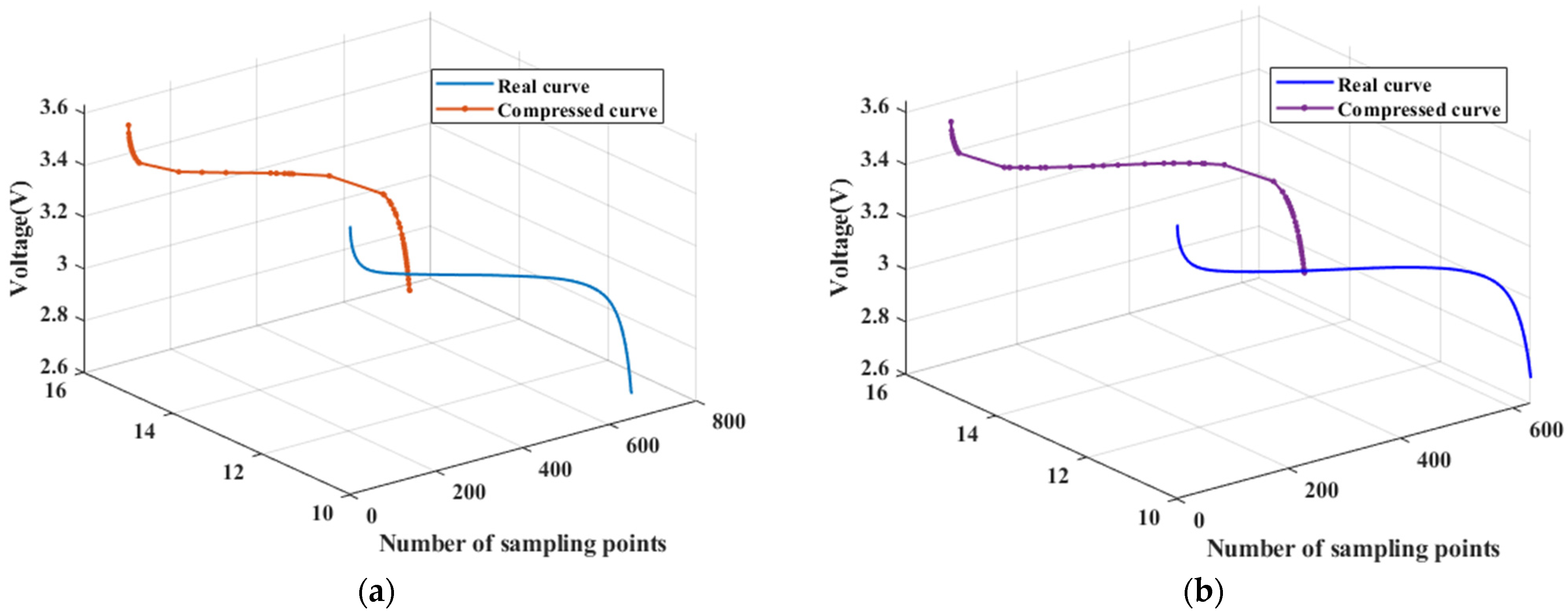
The experimental results in Figure 12 demonstrate that the proposed threshold selection method, which replaces the classical dip-limit algorithm thresholds ${\epsilon }_1$ and ${\epsilon }_2$ with the mean curvature value ${\epsilon }_K$, outperforms the traditional methods shown in Figure 8. The mean curvature value provides a more accurate reflection of the deviation of the original curve from the straight line, resulting in a better fitting and more accurate representation of the original curve’s elevation characteristics, despite the slight increase in the number of feature points.

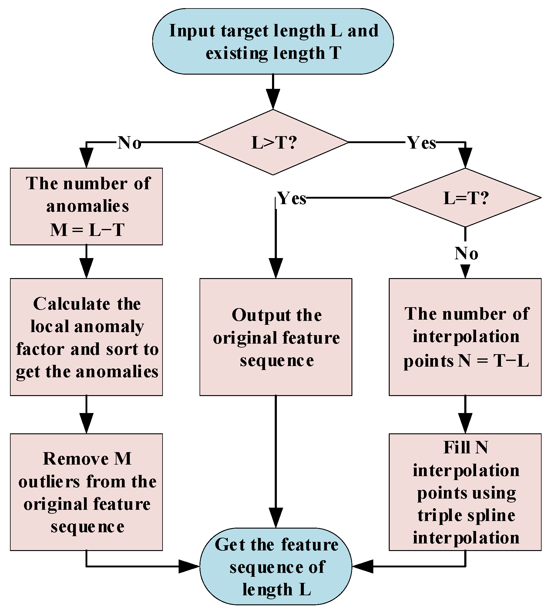
5.3. Length Normalization Based on Cubic Spline Interpolation and Outlier Detection

To ensure that the curves have the same length for input into the prediction model, it is necessary to perform length normalization since the lengths of the curves in different cycles are not the same and the curvature thresholds ${\epsilon }_K$ on different curves are calculated differently. The feature points extracted from each curve after processing using the method described in the previous section have dimensionalities. The normalization process is shown in Figure 13.

5.3.1. Cubic Spline Interpolation to Add Feature Points

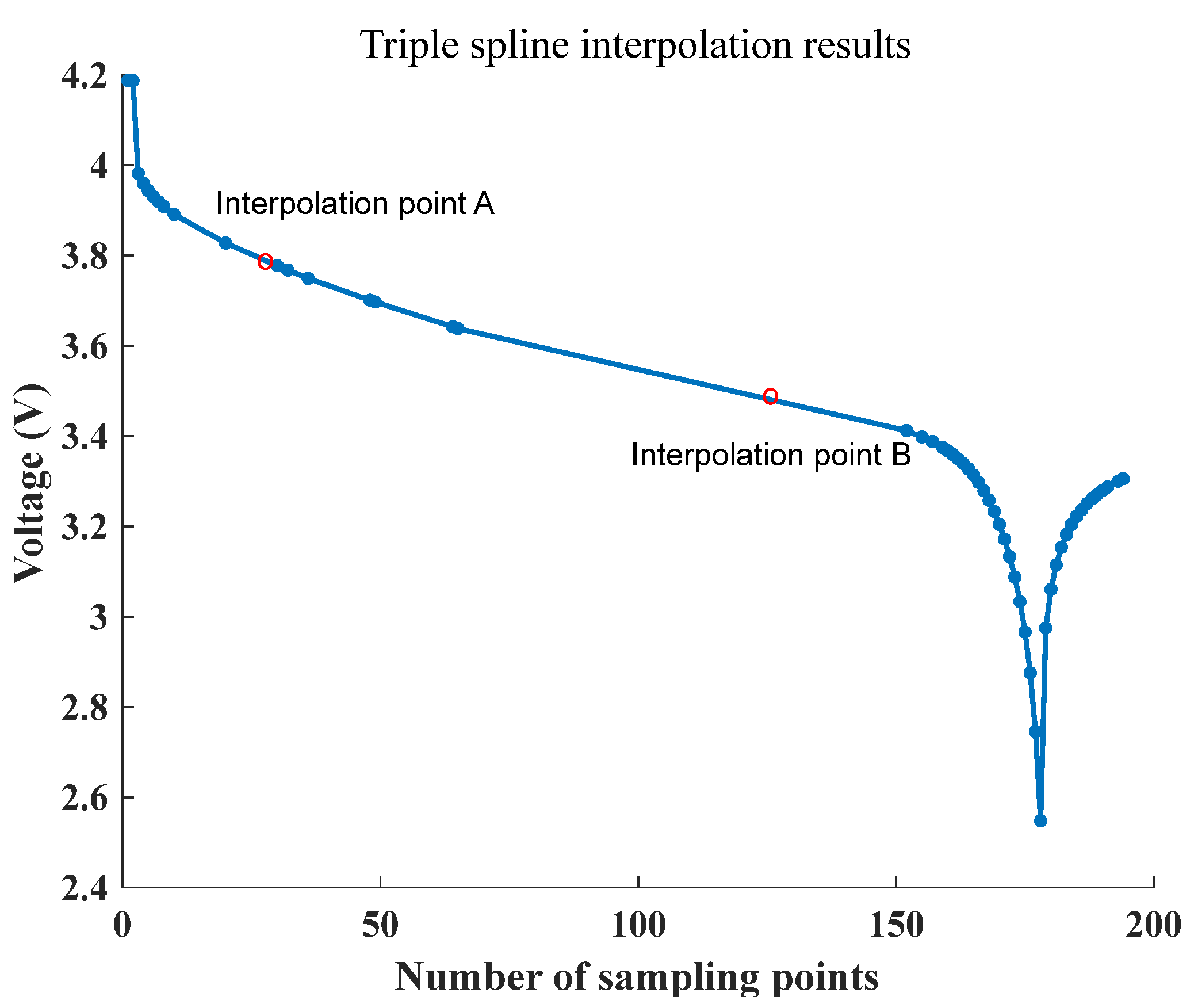
To obtain a fixed-length feature sequence of L, this study employs cubic spline interpolation to split the original long sequence into several segments, constructing multiple cubic functions. This method enables the segments to process gentle articulation at the joints of the segments while retaining the maximum information of the original feature curve. Sequences of less than L length are added to the feature sequence while ensuring the maximum information of the original feature curve is preserved. Figure 14 shows the interpolation result of the compressed curve, where the original compressed curve has a length of 53 and is now randomly filled into a feature sequence of length 55.

Figure 14 illustrates that the interpolation points A and B of the curve, which were obtained using cubic spline interpolations, are distributed along the fitted curve, indicating that the interpolation points do not have a significant impact on the elevation characteristic distribution of the original feature curve.

5.3.2. LOF Anomaly Detection to Remove Feature Points

To reduce data points in feature sequences exceeding length L, excess feature points need to be removed, and the local density feature is calculated to reflect the abnormality degree of certain samples. The LOF method is a prominent density-based outlier detection technique that calculates LOF numerically to reflect the abnormality degree of a sample. using the following equations:

For two points in the sample, the reachable distance from $x^{(i)}$ to $x^{(j)}$ can be expressed as follows:

$$R{D}_{(t)}(x^{(i)},x^{(j)})=\max (||x^{(i)}-x^{(k=t)}||,||x^{(i)}-x^{(j)}||)$$

(13)

where $k$ denotes the distance neighborhood length.

Assuming there are $M$ sample points in the $k$ distance neighborhood of $x^{(i)}$, denoted by $x_M$, the locally reachable density of $x^{(i)}$ can be expressed as follows:

$$LR{D}_k(x^{(i)})=(\frac{1}{M}{\displaystyle \sum _{t=1}^{M}R{D}_k(x_M^{(t)},x^{(i)})})$$

(14)

where $x_M^{(t)}$ denotes the $t$ sample point in $x_M$. The smaller the local reachable density of $x^{(i)}$, the further away the point $x^{(i)}$ is from its neighborhood, and the higher the probability of it being an anomaly. The local anomaly factor is defined as the ratio of the average density of the sample points around a sample point to the density of the location of the sample point. LOF can be expressed as follows:

$$LO{F}_k(x^{(i)})=\frac{({\displaystyle \sum _{t=1}^{M}LR{D}_k(x_M^{(t)})})/M}{LR{D}_k(x^{(i)})}$$

(15)

The numerator in Equation (15) represents the mean of the locally reachable density of $x^{(i)}$ in the distance between $k$ and all sample points in the neighborhood, while the denominator is the locally reachable density of $x^{(i)}$. When the density of $x^{(i)}$ is lower than that of the surrounding samples, the Locally Reachable Density $LR{D}_k(x^{(i)})$ is smaller, leading to a higher $LO{F}_k(x^{(i)})$ value than one. This indicates that the density of the location of $x^{(i)}$ is lower than that of the surrounding samples, making it more likely to be an abnormal sample point. The feature sequences that exceed the length of L are detected as outliers, and redundant feature points are removed. 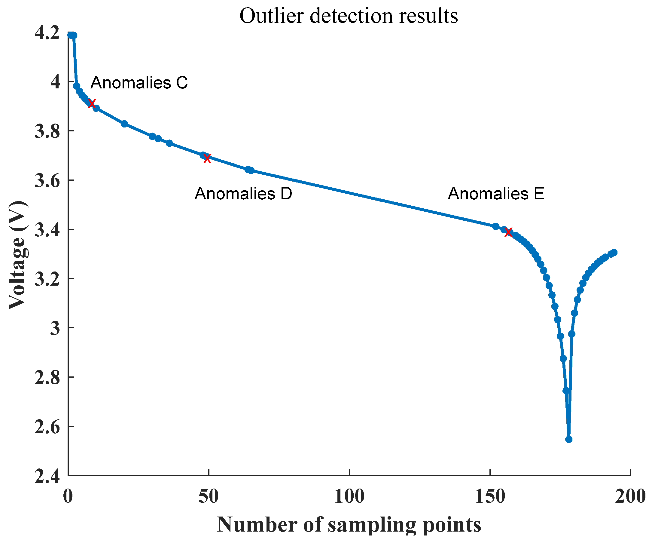The results of outlier detection on the original feature sequence are illustrated in Figure 15. The original feature sequence has a length of 53, and by removing the top three feature points with the largest local anomaly factor, a feature sequence of length 50 is obtained.

The results in Figure 15 demonstrate that the curve maintains its original shape after LOF anomaly detection and removal. This process reduces the length of the feature sequence and achieves length normalization while still retaining the maximum feature information. Therefore, the proposed method effectively detects and removes outliers from the original feature sequence without significantly affecting the overall shape of the curve.

5.3.3. Determination of the Optimal Length L

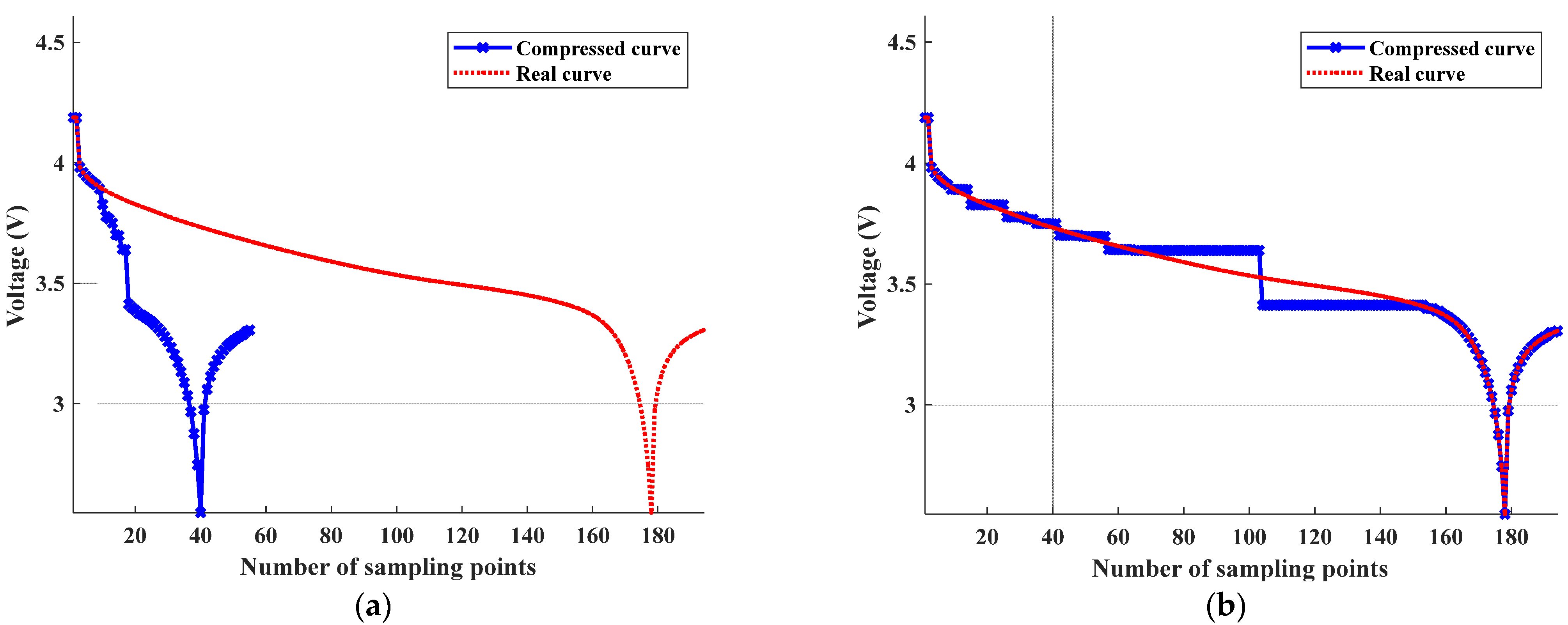
To determine the final feature length L, the Dynamic Time Warping (DTW) algorithm is used to evaluate the temporal similarity between the compressed curve and the original curve. The DTW algorithm employs a dynamic planning strategy that performs a dynamic time-domain regularization process on two, time series to find the minimum possible distance (i.e., maximum possible similarity) between them. The degree of deformation in the time domain between two, time series that are otherwise similar is not only time-varying but also nonlinearly varying. Figure 16a illustrates this by showing that the compressed curve and the true curve exhibit different degrees of deformation in the time domain while still having high time similarity. To accurately determine the similarity between the two curves, it is necessary to first perform relative deformation and correction of the local time-domain waveforms between them, which involves implementing dynamic regularization, and then calculating the Euclidean distance, as shown in Figure 16b.

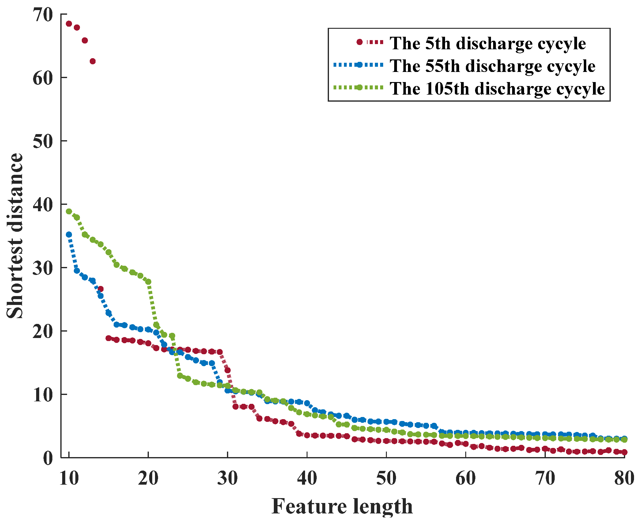
After the dynamic time-domain regularization and estimation of the shortest distance between the two sequences, the time-domain waveforms in the local ranges of the compressed discharge voltage curves are relatively stretched before they correspond. The trend of the shortest distance between the discharge voltage curves in the 5th, 55th, and 105th cycles with different feature sequence lengths and the original curve after processing by the method described earlier is illustrated in Figure 17. The optimal feature length L is determined by analyzing the variation of the minimum value.

The amount of feature information in a dataset is directly proportional to its dimensionality. Higher dimensionality leads to more feature information, while lower dimensionality results in reduced feature information. Figure 17 shows that the minimum distance value between the compressed curve and the original curve gradually decreases as the feature point length L decreases. The minimum distance between the curves reaches a plateau when the feature point length L is approximately 40, and it remains constant thereafter. Therefore, for the discharge voltage curves across multiple cycles, the feature sequence length L is fixed at 40. Similarly, the optimal feature sequence length is determined using the improved altitude method for the voltage, current, and power curves in the charging experiment as well as the current and power curves in the discharge experiment.

The proposed method effectively extracts the most essential feature information from the dataset, determines the optimal length of the characteristic sequence, and ensures that the feature sequences have the same length for easy input into the prediction model. This approach mitigates the impact of dimensionality and leads to accurate SoH and RUL prediction results.

In summary, the proposed method provides an effective means of extracting critical information from the dataset and facilitating accurate predictions of SoH and RUL.

5.4. SoH Prediction Based on the CatBoost Model

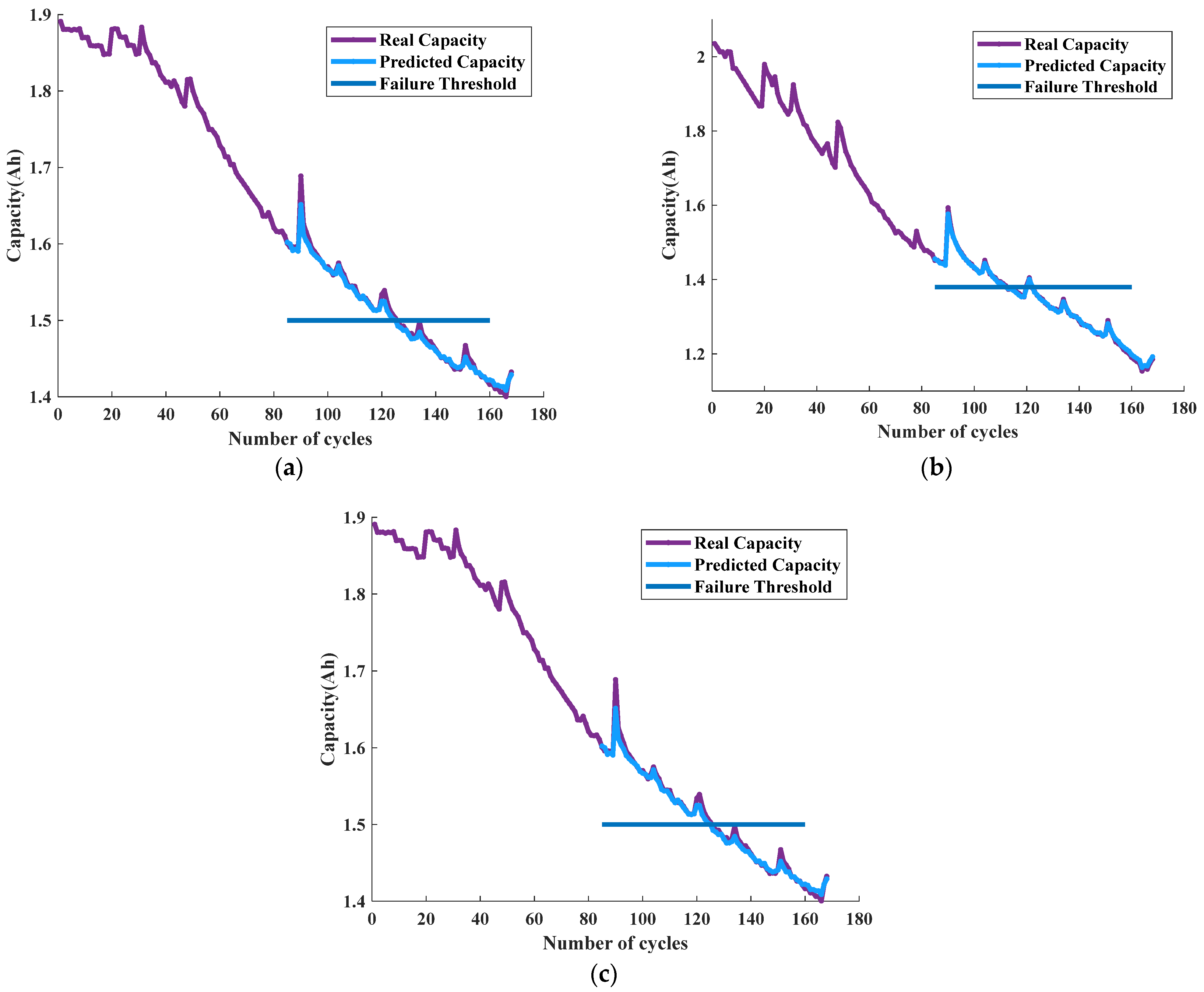
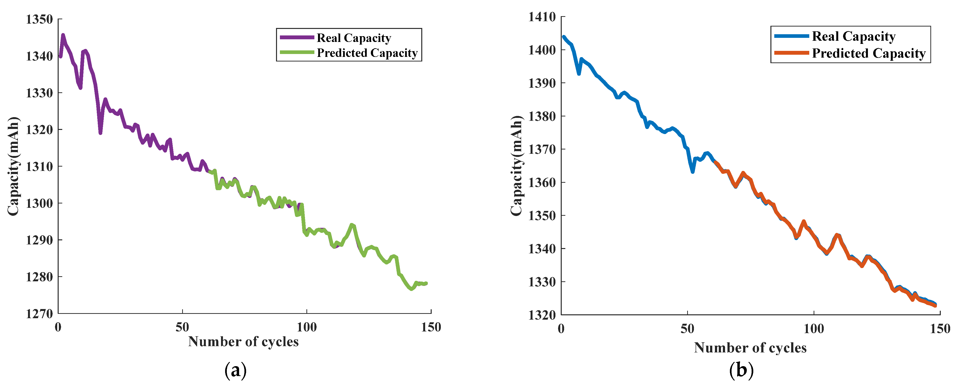
Following the curve compression and feature length normalization, the resulting features were used as input to the CatBoost model for predicting the State of Health (SoH) of the batteries. For the 168 cycles of batteries B0005, B0006, and B0007 obtained after feature processing, the first 84 cycles were used for training, while the remaining 85th to 168th cycles were used for testing. The prediction model established in the previous section was employed to predict the SoH and Remaining Useful Life (RUL) of the three sets of batteries. The test set prediction results for both SoH and RUL are illustrated in Figure 18, indicating the effectiveness of the model for accurately predicting the SoH and RUL of each battery set.

The findings illustrated in Figure 18 indicate that the prediction curves obtained from the model closely match the test set results for dataset A. The significant overlap between the predicted curves and the true capacity curves is evidence of the model’s ability to accurately forecast both the State of Health (SoH) estimation and Remaining Useful Life (RUL) prediction for dataset A. This suggests that the model is highly effective in accurately predicting battery capacity and can be employed to reliably forecast the SoH and RUL of batteries.

To assess the accuracy of the prediction models for each battery, several evaluation metrics are used, including Mean Square Error (MSE), Mean Absolute Error (MAE), Root Mean Square Error (RMSE), and goodness-of-fit ($R^2$).

Table 2. Specific information on predictive evaluation indicators.

Battery Number	MSE	RMSE	MAE	AE	${\mathit{R}}^2$
5	3.7248 × 10−5	0.0061	0.0052	0	0.9967
6	2.1665 × 10−5	0.0047	0.0040	1	0.9915
7	9.2121 × 10−5	0.0030	0.0026	0	0.9883

provides detailed information regarding the prediction evaluation metrics, such as error distribution, while Figure 19 illustrates the SoH prediction error distribution. The evaluation metrics are calculated based on the following equations:

$$MSE={\displaystyle \sum _{i=1}^N\frac{1}{N}}{(f(x_i)-y_i)}^2$$

(16)

$$MAE=\frac{1}{N}{\displaystyle \sum _{i=1}^N|f(x_i)-y_i|}$$

(17)

$$RMSE=\sqrt{\frac{1}{N}{\displaystyle \sum _{i=1}^N{(f(x_i)-y_i)}^2}}$$

(18)

$$R^2=1-\frac{{\displaystyle \sum _{i=1}^N{(f(x_i)-y_i)}^2}}{{\displaystyle \sum _{i=1}^N{(f(x_i)-y_{mean})}^2}}$$

(19)

where $f(x_i)$ denotes the true value, $y_i$ denotes the predicted value, $i=1,2,\dots ,N$, $N$ denotes the sample size, $R^2$ denotes a measure of the overall fit of the regression equation, which has values between [0 and 1], and $y_{mean}$ denotes the mean value of the actual observed values.

The abbreviation AE in

Table 3. Comparison of multi-model prediction effects.

Predictive Models	Battery Number	MSE	RMSE	MAE	AE	${\mathit{R}}^2$
Random Forest	5	0.0030	0.0546	0.0442	4	0.9602
	6	8.9984 × 10−4	0.0300	0.0238	3	0.9769
	7	0.0072	0.0850	0.0755	2	0.9713
XGBoost	5	1.3301 × 10−4	0.0115	0.0084	2	0.9808
	6	6.2771 × 10−4	0.0251	0.0195	1	0.9813
	7	1.3129 × 10−4	0.0115	0.0086	2	0.9689
CatBoost	5	3.7248 × 10−5	0.0061	0.0052	0	0.9967
	6	2.1665 × 10−5	0.0047	0.0040	1	0.9915
	7	9.2121 × 10−5	0.0030	0.0026	0	0.9883

represents the absolute error, which is the absolute difference between the actual RUL and the predicted RUL of each battery.

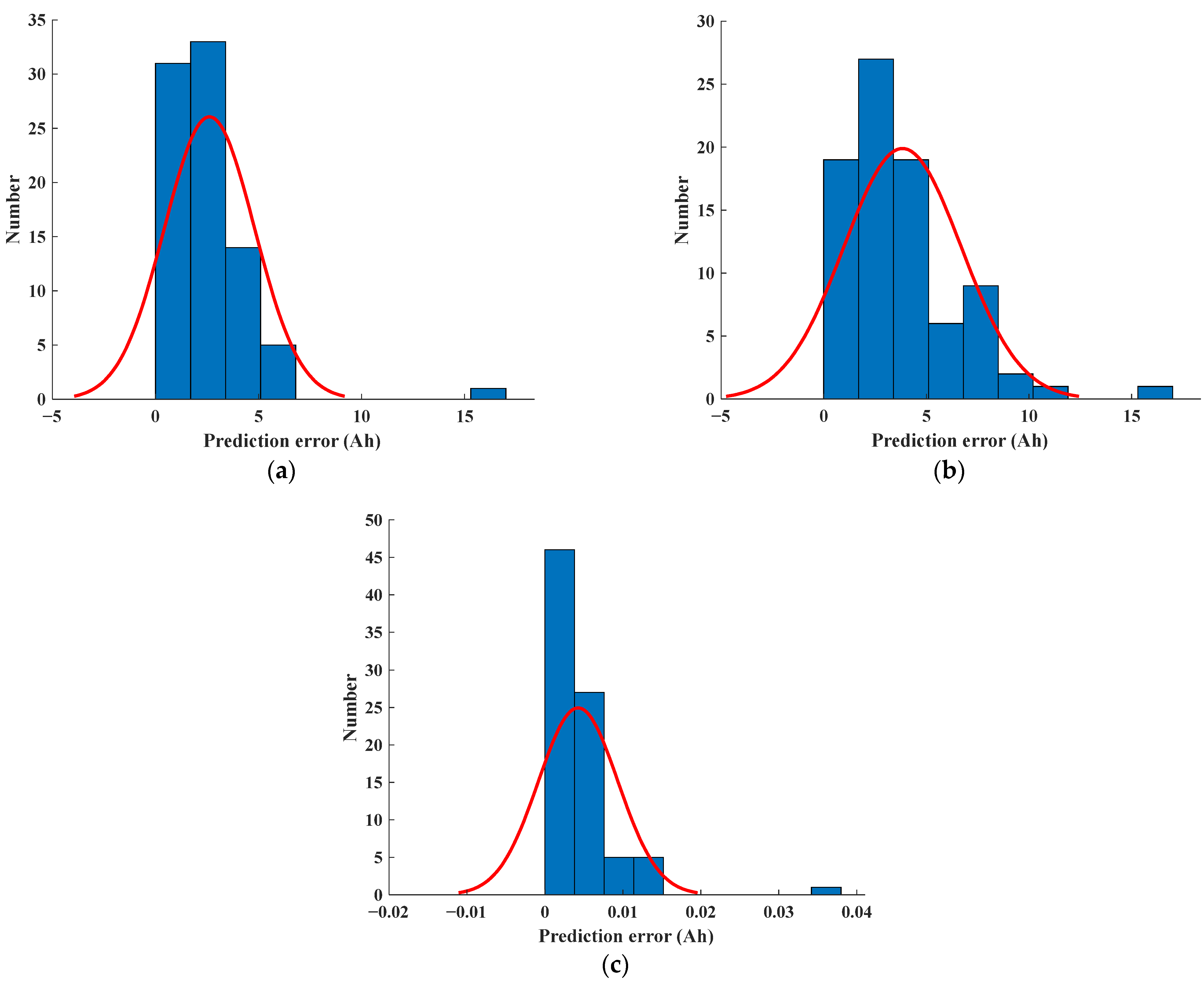
Figure 19 depicts the error distribution of the predicted Remaining Useful Life (RUL) for batteries five, six, and seven. The horizontal axis displays the difference between the predicted and actual RUL values, while the vertical axis indicates the frequency of occurrence for each error interval. Analysis of both Figure 18 and Table 2 reveals that the error intervals for all three batteries exhibit a primary concentration between 0 and 0.05. Additionally, battery number five demonstrates a low error rate, with the majority of the errors falling below 1 × 10⁻³. These results indicate that the proposed feature engineering and CatBoost model utilized in this study have significant advantages in the realm of State of Health (SoH) estimation.

5.5. Comparison of the Effects of Different Models

In order to confirm the efficacy of the CatBoost model employed in this study, we conducted a comparative analysis between our chosen model and two other models, namely the Random Forest and XGBoost models. For this analysis, we inputted the capacity features obtained in the previous section and compared the performance of each model in predicting the SoH and RUL of the batteries. The results of this analysis are presented in Table 3. This comparison enabled us to validate the superiority of the CatBoost model in accurately predicting the SoH and RUL of the batteries as compared to the other two models.

Table 3 shows that CatBoost, XGBoost, and Random Forest algorithms all exhibit good regression prediction ability, with their goodness-of-fit and RMSE being relatively close, indicating the good adaptability of the feature engineering approach used in this study. However, the average MSE value of CatBoost for the three batteries (5.0345 × 10⁻⁵) is significantly lower than that of Random Forest and XGBoot. Additionally, the prediction goodness-of-fit of the CatBoost model is better; the average value of $R^2$ is 0.9922, improved by 0.0228 and 0.0152, respectively. Therefore, the CatBoost method can effectively enhance the accuracy of SoH estimation and operational efficiency and exhibit good performance in SoH estimation.

5.6. Model Generalizability Validation

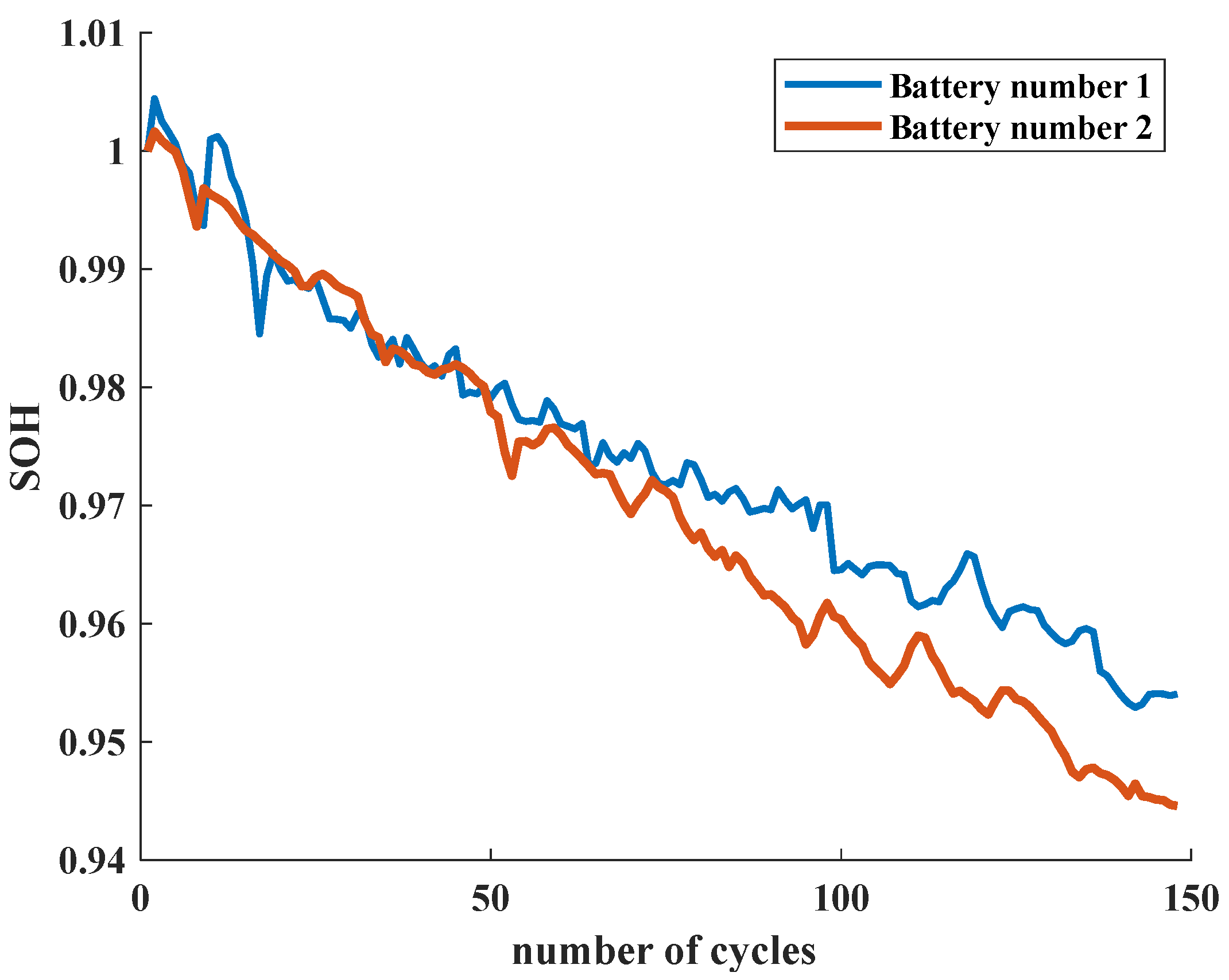
To verify the generalization ability of the feature engineering and prediction model proposed in this study, feature extraction is conducted again for dataset B, and SoH prediction is performed using the CatBoost model. Dataset B comprises two batteries, each with 148 cycles. The first 60 cycles are used as the training set, and the remaining 88 cycles are used as the test set. The model established in the previous section is used for training and prediction. Figure 20 presents the discharge voltage curve of battery number two in dataset B.

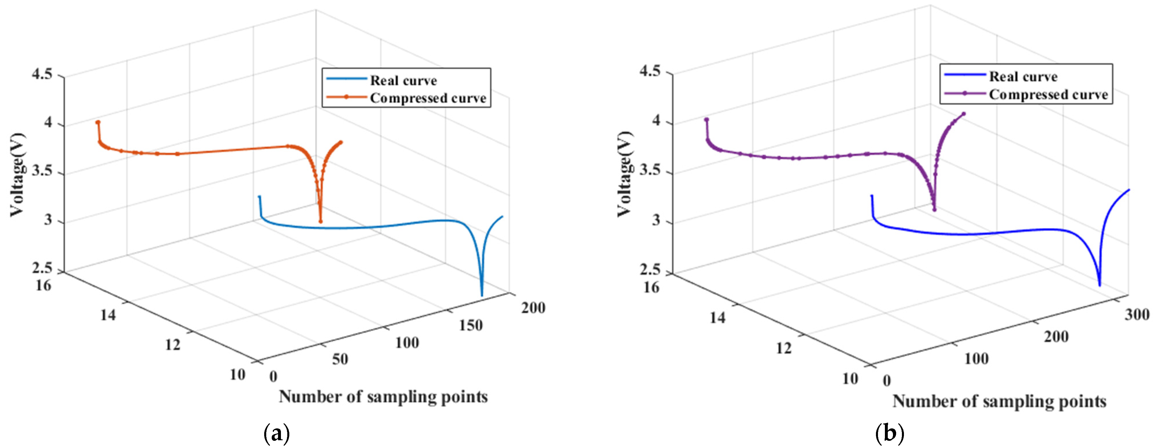
Similar to dataset A, the discharge voltage curves in dataset B have non-uniform sampling lengths under different cycles and cannot be directly used as feature input. Therefore, following the method described in the previous section, suitable gentle curve segments are selected, and the mean curvature value is calculated to serve as a judgment threshold. This threshold is then used to compress the discharge voltage curves for each cycle using the drape limit algorithm. Figure 21 displays the compression results of the discharge voltage curves in the 1st cycle and the 61st cycle for battery number two among the cycle data.

After length normalization and similarity comparison, a feature sequence with a length of 50 is obtained. The model established in the previous section is then used for training and predicting. The prediction results are shown in Figure 22.

Based on Figure 22, it is evident that the CatBoost model outperforms the other models in the feature engineering approach proposed in this study for the two batteries in dataset B. In battery number one, the model has an MSE value of 0.2011 and an MAE value of 0.3761, with a goodness-of-fit of 0.9986. For battery number two, the model has an MSE value of 0.1031 and an MAE value of 0.2655, with a goodness-of-fit of 0.9997. These results demonstrate that the model can accurately predict SoH for the same battery.

In summary, the curve compression-based approach and the CatBoost prediction model proposed in this study both demonstrate good prediction accuracy in different datasets, indicating that the model established in this study exhibits strong generalization ability.

5.7. Model Robustness Verification

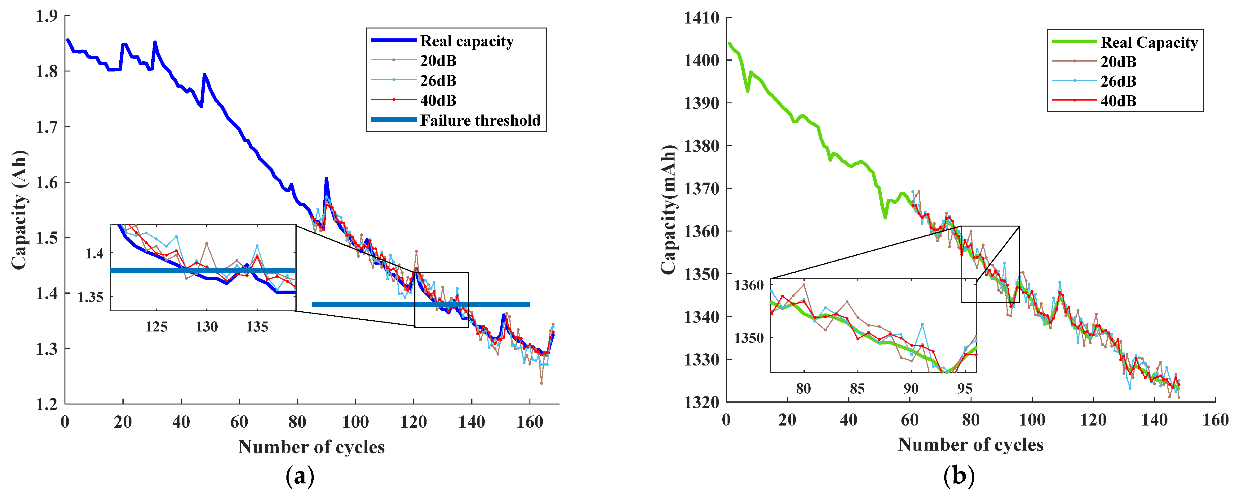
In order to evaluate the performance of the prediction model in real-world sampling environments, robustness experiments were conducted to test its resilience. Gaussian White Noise (GWN) was added to the test set as an interference signal to observe the behavior of the model in the presence of noise with different Signal-to-Noise Ratios (SNRs). A GWN with varying noise ratios, ranging from 1% to 10%, was selected and converted to SNRs before being added to the test set to assess the model’s ability to resist interference. The prediction of Battery B0005 in dataset A and Battery number two in dataset B were taken as examples, and Figure 23 presents the prediction results obtained under different SNRs. This enabled us to evaluate the robustness and effectiveness of the prediction model under varying conditions, thereby confirming its ability to perform accurately even in the presence of noise and interference.

The performance of the curve compression-based approach and CatBoost model proposed in this study under noisy conditions is demonstrated in Figure 23. After the addition of interference signals, the predicted curves exhibit some fluctuations and deviations from the true path. However, for cell B0005 in dataset A, as shown in the local enlarged figures, RUL prediction errors are within two cycles, and the goodness-of-fit ($R^2$) values are all above 0.95. When SNR is relatively high, especially at SNR = 40 dB, the model’s prediction is hardly affected, with an $R^2$ value of 0.9817. For cell two in dataset B, it still works well in the noisy environment with a good prediction curve fit. These results indicate that the prediction model proposed in this study has strong adaptability, anti-interference capabilities, and robustness.

6. Conclusions

To address the issue of low accuracy in SoH and RUL prediction arising from the difficulty in establishing feature engineering for lithium-ion batteries, this study proposes a SoH and RUL prediction model based on curve compression and CatBoost. Relevant experiments were conducted, leading to the following conclusions:

(1) The improved perpendicular distance threshold algorithm proposed in this study can capture battery aging information to the maximum extent. The improved threshold selection method does not require manual threshold setting, as the algorithm automatically determines the gentle curve segment based on the derivative and calculates the mean curvature value based on the deviation of this curve segment from the straight line, thereby exhibiting universality across different curves. Additionally, the length normalization method based on cubic spline interpolation and outlier detection can effectively standardize data length while retaining feature information.

(2) In the field of battery SoH estimation, the feature engineering and prediction model proposed in this study have demonstrated accurate prediction capabilities. In dataset A, the battery model exhibited an $R^2$ value higher than 0.98. In dataset B, the feature engineering and model established in this study also produced better prediction results, demonstrating the good generalization of the proposed method.

(3) The CatBoost model utilized in this study revealed significantly better prediction performance than other models. The $R^2$ is improved by 0.0228 and 0.0152 compared to the Random Forest algorithm and XGBoost, respectively.

(4) The curve compression-based approach and the CatBoost model proposed in this study were shown to be almost unaffected by the presence of noise in terms of prediction accuracy, indicating that the model exhibits strong anti-interference capability and robustness.