Determination of the Reliability of Urban Electric Transport Running Autonomously through Diagnostic Parameters

Abstract

The urban transport network involves complex processes, operating 24 h a day and 365 days a year. The sustainable development of the urban transport network using electric buses and trolleybuses that run autonomously is an urgent task since the transport network performs integral social functions and is the transport artery of any urban center. The social and economic life of a city as a whole depends on the reliability of the transportation network. A theory is proposed for the technical and economic evaluation of reliability improvement in electric buses and trolleybuses running autonomously, which enables the determination of the reliability parameters of electric buses and forecasts for the future from the point of view of optimal economic costs for the operation of electric equipment in electric buses. As a result of the application of the proposed theory, it was found that increasing the reliability of the transportation fleet can lead to a decrease in both specific operating costs and capital investments in the development of the fleet. This is achieved as a result of increasing the annual productivity of vehicles by reducing the time they are out of service to eliminate the consequences of failures and carry out maintenance and repair. The conducted experiments confirmed that the theory and methodology of optimal reliability level selection not only enable the rational use of the material resources of the urban transport network but also the release of funds for its scientific and technical development by reducing the number of failures in the electrical equipment of transport systems by 14%.

1. Introduction

The growth of transport infrastructure and the rolling stock of trolleybuses and electric buses in cities with high population densities and heavy traffic have led to acute urban planning, socio-economic, and environmental problems [1,2]. The main concepts of sustainable development in urban transportation assume sustainable development and improvement of the transport fleets of cities [3]. This requires the development of reliable, uninterrupted, and comfortable vehicle operation [4,5,6]. Therefore, the quantitative transport indicator—the annual number of trips of one person on public transport—was included in the comfort ratings of cities in Europe and Asia. Under the new conditions, more and more high requirements are imposed on public transport [7,8]. First of all, it should be attractive and reliable for the user, which requires the creation of appropriate criteria [9]. Improving the quality of public urban passenger transport services is the basis for the quality of passenger traffic, a factor of its stability, and the most important task of development in modern cities and agglomerations [10]. Decisions made in this area are aimed at improving the reliability of the city’s transport system and road safety, as well as ensuring high environmental standards for the urban environment. In fact, we are talking about improving the social standard of transport services for passengers and luggage transportation through urban ground-based electric transport, which includes benchmarks for the quality and reliability of passenger transport and its infrastructure [11,12].

The novelty of this work consists of the research and development of new approaches to diagnostics and reliability improvement in trolleybus equipment, enabling reductions in unscheduled failures and downtime between repairs, which, in turn, will reduce total operating costs and thus free up funding for the development of trolleybus depots.

This paper considers indicators for assessing the reliability of the urban passenger system [13,14], such as the probability of failure-free operation, failure rate, and electrical equipment (EE) testability, which is understood as EE adaptability to diagnostic work that provides the necessary reliability under given conditions with minimal labor, time, and cost. The evaluation of equipment testability is especially important for older vehicle models that do not have developed intelligent information interfaces and built-in diagnostic sensors.

When working on the paper, the initial statistical information on equipment failures and monitoring technical information used in diagnosing the current technical condition was obtained on the basis of modern rolling stock equipment (GPS navigation systems, various on-board diagnostic systems with wireless data transmission, diagnostic benches in depots). The limitations of the current study are that the information period of the statistical database of equipment failures of trolleybuses and electric buses was only four years, from 2019 to 2022, as well as well as the fact that, in the mathematical model, equipment failures were assumed to be independent of each other and not affecting the performance of other equipment.

In this paper, the following tasks were set to improve the reliability and stability of the transport network using electric buses and trolleybuses running autonomously:

• Assessment of the possibility of operational control of the electrical equipment of autonomous trolleybuses and electric buses. Such an assessment is an important step in the overall assessment of the reliability of the electrical engineering complex of electric transport.
• Estimation of the characteristic of electric equipment reliability through indicators that characterize the number of equipment failures per unit of mileage, i.e., through the flow of failures and through the probability of no-failure operation.
• As a result of the analysis of existing methods for modeling the state of electrical equipment, on the basis of the maximum likelihood method, proposing a modeling method based on the selection of a universal equalizing function for most types of electrical equipment in the trolleybus electrical complex.
• Need for developing approaches enabling the creation of a system for monitoring and forecasting the technical conditions of electric transport. The monitoring system should be integral probabilistic–diagnostic and allow for the continuous monitoring of the performance of the equipment of electric transport in use.
• Proposition of a comprehensive method for evaluating and predicting performance.
• Development of standards and provisions for accident-free and failure-free operation of the electric equipment of electric transport in use.
• Development of a method to economically evaluate the trolleybus electrical complex reliability improvement, considering the costs of the creation and operation of the electrical equipment.

The structure of the paper is as follows: Section 1 highlights the relevance and importance of the problems, the objectives of the study, and the reliability prediction of trolleybus and electric bus equipment; Section 2 describes the data description and methodology; Section 3 presents the results of the study; Section 4 provides a discussion of the results obtained; Section 5 provides conclusions.

2. Data Description and Methodology

In order to approach the evaluation and improvement of EE reliability in trolleybuses and electric buses, we will consider the issues of evaluating the testability of the electrical equipment of the vehicles as fundamental for further research.

One way to increase the availability and utilization rates of the vehicles is a reduction in their downtime for maintenance and repair, which is provided by increasing the percentage of control and diagnostic works in the total volume of maintenance and repair work. The increase in control and diagnostic work in the process of vehicle maintenance is especially noticeable. The volume of control–diagnostic and adjustment works exceeds 25–30% of the total volume of vehicle maintenance works. As a rule, the useful time spent on the direct measurement of diagnostic and controlled parameters on average is equal to 5–10% of the total time of diagnostics; the other 90–95%is spent on installation and the removal of primary converters, the establishment of the necessary mode of vehicle operation for the diagnostics, and the processing of the diagnostic results. And the removal and installation of transducers account for up to 50–80% of the total time of diagnostics.

An important way to reduce the labor intensity of control and diagnostic works is to increase the testability of vehicles, including their adaptability to diagnostics and the introduction of more effective methods of control and diagnostics.

It is known that the distribution of random variables for trolleybus electrical equipment failures can be described by the law of normal distribution [14].

The normal distribution of a random variable (a Gaussian distribution) is a probability distribution. The Gaussian distribution in the one-dimensional case is given by a probability density function. This probability density function coincides with the Gaussian function:

$$f(x)=\frac{1}{\sigma \sqrt{2\pi }}{e}^{-\frac{1}{2}{\left(\frac{x-\mu }{\sigma }\right)}^2}$$

where μ is the mathematical expectation (mean), mode, and median of the distribution;

σ is a standard deviation;

σ² is a distribution variance.

• In the case of material degradation, the mathematical expectation can be written in the following form:

$$L_o=\frac{{\displaystyle \sum _{i=1}^k{L}_i·m_i}}{{\displaystyle \sum _{i=1}^k{m}_i}}$$

where $L_i$ is the mileage of equipment in the $i$-th category, in h;

$m_i$ is the number of sample splits in the $i$-th digit;

$k$ is the number of categories.

2.

The path dispersion is

$$D={\sigma }^2=\frac{{\displaystyle \sum _{i=1}^k{\left(L_i-L_o\right)}^2·m_i}}{{\displaystyle \sum _{i=1}^k{m}_i}}$$

3.

With respect to the selected trajectory or scatter, the standard deviation will be calculated as:

$$\sigma =\sqrt{D}=\sqrt{\frac{{\displaystyle \sum _{i=1}^k{\left(L_i-L_o\right)}^2·m_i}}{{\displaystyle \sum _{i=1}^k{m}_i}}}$$

4.

The variation coefficient is determined by the formula:

$$V=\frac{\sigma }{L_o}$$

An important characteristic of equipment degradation can be calculated when the maximum number of its failures occurs. This characteristic can be calculated by combining the data obtained from two sources. The first is the processing of statistical information using the formulas given above. And the second is the calculation of the numerical characteristics of trolleybus equipment degradation.

The maximum number of equipment failures is characterized by the mathematical expectation of degradation, $L_o$. The possible spread of degradations is shown by the spread, $\sigma$, and the variation coefficient, $V$.

2.1. Assessment of Electrical Equipment Testability

The EE testability implies the adaptability of the EE equipment to diagnostic work, providing, under given conditions, the necessary reliability at a minimum cost of labor, time, and money [15].

Testability is an integral part of trolleybus operational manufacturability. Improving testability requires a system of evaluation indicators based on the labor intensity of diagnostic work and the methodology of applying these indicators in the design, construction, and testing of trolleybuses. The labor intensity of the trolleybus diagnostics consists of the labor intensity of preparatory work, $T_{add}$, (additional labor intensity) and the labor intensity of the diagnostics themselves, $T_0$ (basic labor intensity), including the measurement of the diagnostic parameters and the diagnostic settings. $T_{add}$ mainly depends on the improvement in the EE design, and $T_0$ depends on the quality of the diagnostic methods and tools. At the same time, both $T_0$ and $T_d$ are determined by the indicators of equipment reliability and cost.

The noticeable stabilization of trolleybus diagnostics in recent years has enabled us to assume that testability is mainly developed by ensuring a periodic acquisition of information about the technical condition of the EE during its maintenance, i.e., by reducing $T_{add}$.

In the future, testability will be developed mainly by providing trolleybuses with built-in devices that continuously record and accumulate information about their technical condition. This will lead to corresponding changes occurring in the methods and means of external diagnostics and will require their automation, which will reduce $T_{bas}$.

Developing the methods for calculating the testability indicators of the vehicles enables a reduction in the evaluation of the testability indicators of the EE based on the values of $T_{bas}$ and $T_{add}$. The testability standard, $N$, and the testability coefficient, $K$, were chosen as the main indicators of testability, which characterize it quantitatively.

The testability standard, $N$$\raisebox{1ex}{$\mathrm{man} \mathrm{hours}$}\!\left/ \!\raisebox{-1ex}{${10}^3\times \mathrm{tn}\times \mathrm{km}$}\right.$, comprehensively defines the testability of the EE (and its elements) in direct connection with its reliability, operating conditions, and the control system.

$$N=\frac{T_{bas}+T_{add}}{L_{des}·Q}$$

(1)

where $T_{bas}$ is the basic labor intensity of control and diagnostic work related to measuring parameters and diagnosing, in man-hours; $T_{add}$ is the additional labor intensity due to providing access to the control points by connecting and disconnecting sensors going to test modes, in man-hours. $L_{des}$ is the designated trolleybus mileage, in km; $Q$ is the trolleybus load capacity, which reflects the number of passengers carried (a leading parameter), in t.

The testability coefficient characterizes the suitability of the trolleybus design (its elements and systems) for diagnostics. It enables the level of design solutions in the testability field to be determined completely in the course of both design and testing, but without a cause analysis, i.e., without a qualitative assessment of testability. The testability coefficient is expressed by the ratio:

$$K=\frac{T_{bas}}{T_{bas}+T_{add}}$$

(2)

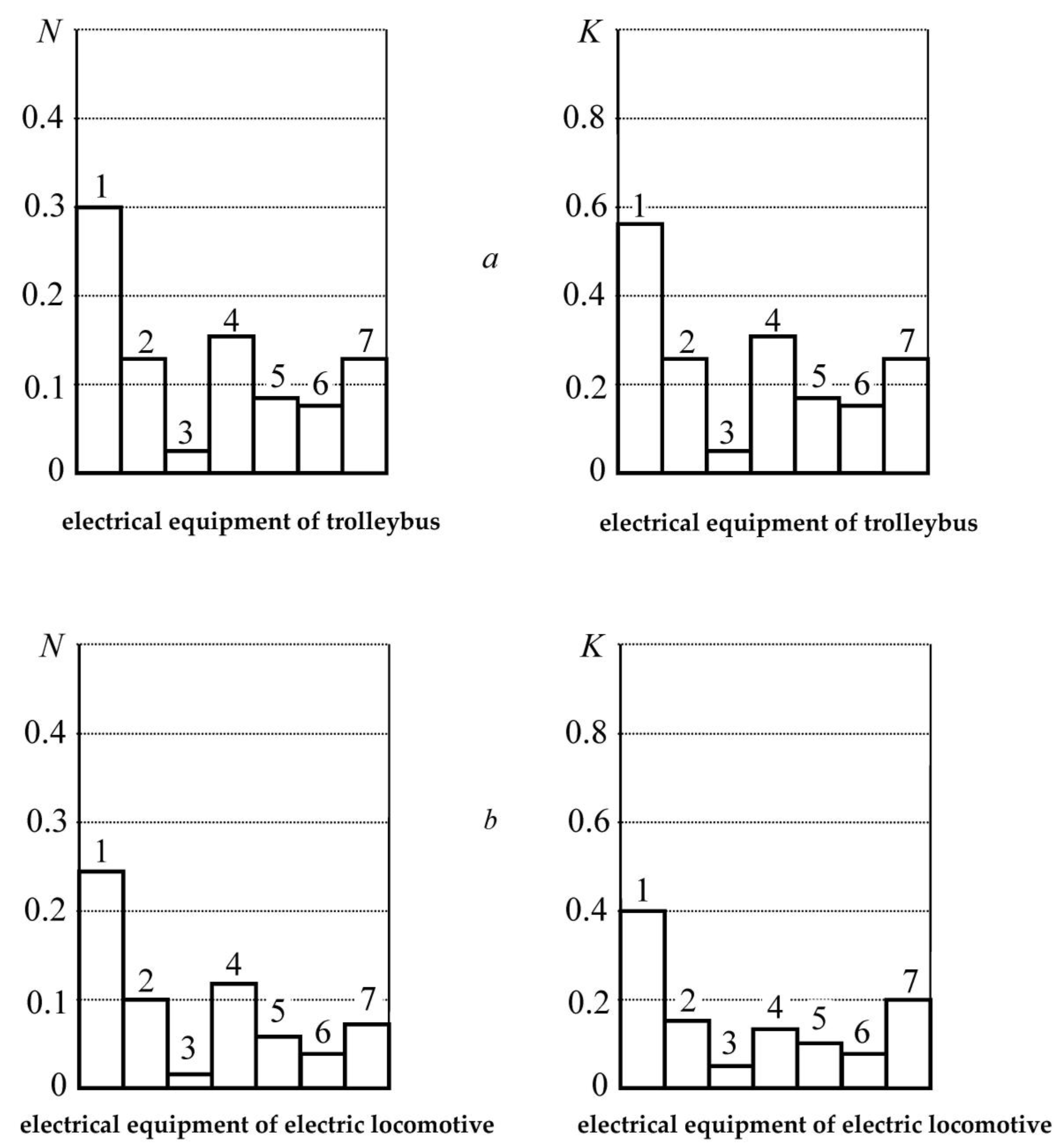
In the course of the research, in the case of a comparative assessment of testability, the EE of a trolleybus and an electric locomotive was analyzed. The calculations performed according to the described methodology and the standards set out in [16,17,18] show that the testability coefficient, $K$, and the testability standard, $N$, are higher for the trolleybus in almost every group and node EE. Figure 1 shows the results of the calculation of the overall testability indices, $N$ and $K$, of the trolleybus and the electric locomotive. Auxiliary electric circuits include circuits for lighting, heating the driver’s cab or saloon, a compressor motor, a fan motor, a heater, and a door mechanism. The trolleybus’ own circuits include power supply circuits for low-voltage control, emergency service lighting, and signaling circuits. The accessory circuits include controllers, voltage converters, a control unit, a power contactor unit, fuses, and an electronic air suspension.

If we compare the trolleybus EE with a similar EE of the modern electric locomotive, the testability of the electric locomotive, as the calculations have shown, is higher because the electric locomotive has all electrical devices with their output terminals brought to the terminal strip, and their work is easily analyzed during diagnostic tests [19]. The currently used trolleybuses have no such circuits, and it is very difficult to obtain information about their operation. This circumstance plays the most significant role in the fact that the trolleybus EE, being a testable device by its structure, is still poorly diagnosed due to the lack of sensor connection points and diagnostic equipment [20,21].

When the trolleybus EEPS operation intensity increases and a labor productivity increase on preventive maintenance is required, the availability of built-in or external EE diagnostics is a significant means of improving testability [22].

The existing rolling stock allows many diagnosed parameters to be controlled by indirect signs. The non-electrical-actuation sound (its frequency and amplitude), heating temperature, the electrical-input resistance in the case of direct current, the frequency dependence of the total input resistance, and others can be used as such signs [23,24].

The paper proposes to modify the design of the trolleybus rolling unit of the manufacturer to improve its EE testability.

In the course of the research and analysis, analyzing the possibility of controlling the EE state in one way or another suggests conditionally dividing its nodes into three groups.

The first group includes the elements and assemblies that can be monitored without being removed from the trolleybus circuitry because they are mostly features that are essential for efficient operation: the control circuit, the traction motor, and the auxiliary electric motors [25].

The second group includes the elements and units for which faults can be detected at a low confidence level without removal from the circuit (removal from the circuit would be preferable for them): the circuit breaker, the generator, the voltage and current relays, the servomotor, the controller, the reverser, and the compressor motor [26].

The third group includes the elements that cannot be checked without being removed: LC—5, 4, the starting and shunt resistors, and the voltage regulator.

In the case of other elements, their removal and individual control are not difficult: batteries and current collectors.

As the main method of trolleybus EE diagnosis, search methods rather than indication methods should be adopted. At the same time, due to the small number of special diagnostic devices installed on a trolleybus, analysis methods based on signs (symptoms) rather than on the diagnosed parameters themselves are currently possible [27,28,29].

In addition, the following maintenance strategy is proposed. The current inspection and diagnostic terms of the trolleybus EE are not optimal, and some units can be in the operating mode for most of the inter-adjustment period when performing maintenance work [30]. In view of this, performing inspections requires performing a minimum of actions in the rheostat group controller, excluding sweeping all the contacts in a row [31]. The running-in period, as calculations have shown, can reach several days, and the disconnection of the running pairs leads to an increase in the probability of its failure [32]. Performing contactor panel diagnostics also requires excluding stripping and adjusting all the contactors and relays.

Newly installed relays and contactors should be singled out. Their resource enables their prevention, diagnosis, and regulation only in the presence of failure or together with others only after the expiration of the resource. It is advisable, in this regard, to keep records of new elements that are installed in contactor panels and group electric apparatuses. This is explained by the sharply differing nature of the reliability decrease in units that are new compared to those formerly in service [33].

As the EE reliability after its partial restoration falls according to the exponential law, an increase in inter-preventive periods will lead only to a weak fall in the EE reliability during operation at an invariable level of control over preventive maintenance [34]. Strengthening the control over failures can considerably reduce the number of failures happening at the optimum inter-protective period, whose value varies within a year from 5.1 to 11 days (

Table 1. Values of an individual MTBF for a given reliability and recovery time of the electrical equipment ($t_d$—diagnostic time, days; ${\overline{P}}_{av}$—average probability of failure-free operation).

${\overline{\mathit{P}}}_{\mathit{a}\mathit{v}}$	$\mathit{T}$ Day
	${\mathit{t}}_{\mathit{d}}=3.5$	${\mathit{t}}_{\mathit{d}}=7$	${\mathit{t}}_{\mathit{d}}=14$	${\mathit{t}}_{\mathit{d}}=28$	${\mathit{t}}_{\mathit{d}}=56$	${\mathit{t}}_{\mathit{d}}=112$	${\mathit{t}}_{\mathit{d}}=224$
0.01	1.031	2.062	4.131	8.271	16.542	33.084	66.169
0.1	2.164	4.328	8.658	17.316	34.633	69.265	138.53
0.2	3.141	6.2822	12.561	25.122	50.244	100.489	200.98
0.3	4.231	8.462	16.927	33.854	67.709	135.42	270.84
0.4	5.592	11.184	22.368	44.737	89.474	178.95	357.89
0.5	7.424	14.849	29.699	59.397	118.79	237.59	475.18
0.6	10.112	20.224	40.441	80.882	161.76	323.53	647.05
0.7	14.522	29.051	58.091	116.18	232.36	464.72	929.45
0.8	23.272	46.541	93.089	186.18	372.36	744.71	1489.4
0.9	49.392	98.797	197.594	395.19	790.38	1580.8	3161.5
0.99	518.79	1037.6	2075.1	4150.3	8300.6	16,601	33,202

).

2.2. Predicting the Electrical Equipment Serviceability

The processes of determining the technical condition, maintaining a given level of reliability of an object, and predicting changes in reliability can be considered a special type of management, which is implemented by means of inspections, faultfinding, and rational maintenance of the trolleybus EE [35].

The method of determining the current technical condition is undoubtedly important under the conditions of changing the reliability of the electrical equipment, $P$, as it enables its current level to be determined (Table 1).

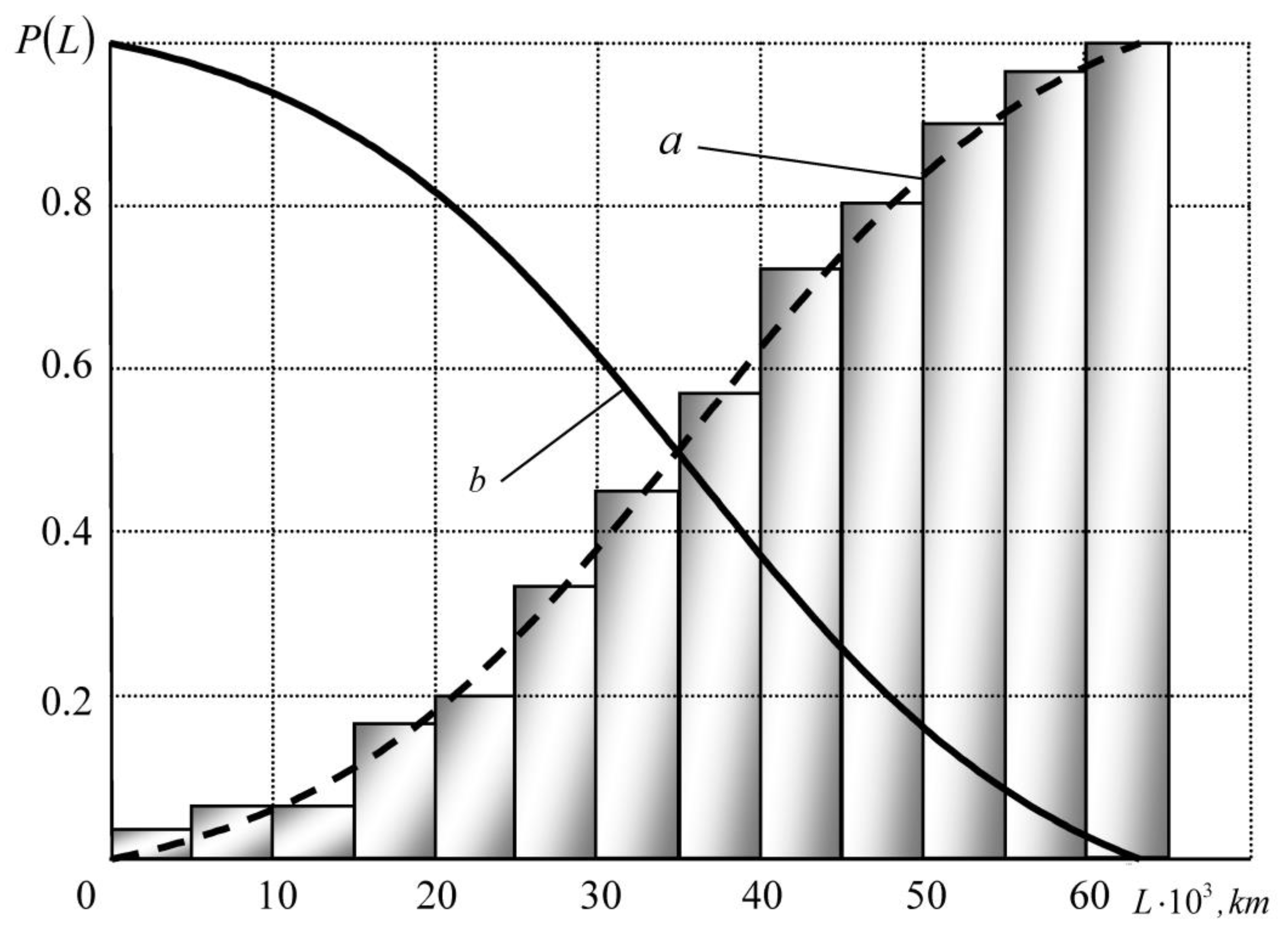
But it is even more important to make predictions about the change in the EE reliability for the future. The stochastic models of statistical modeling obtained (Figure 2 and Figure 3) are recommended to be used for the estimation and forecast of changes in the technical condition of the average statistical EE. So, setting the necessary level of reliability, $P$, enables the time, $t$, or the mileage, $L$, of the normal accident-free operation of the equipment to be determined. At the same time, using the law of reliability change enables the permissible residual time, $t$, or mileage, $L$, of the operation to be specified until the reliability resource is exhausted [36].

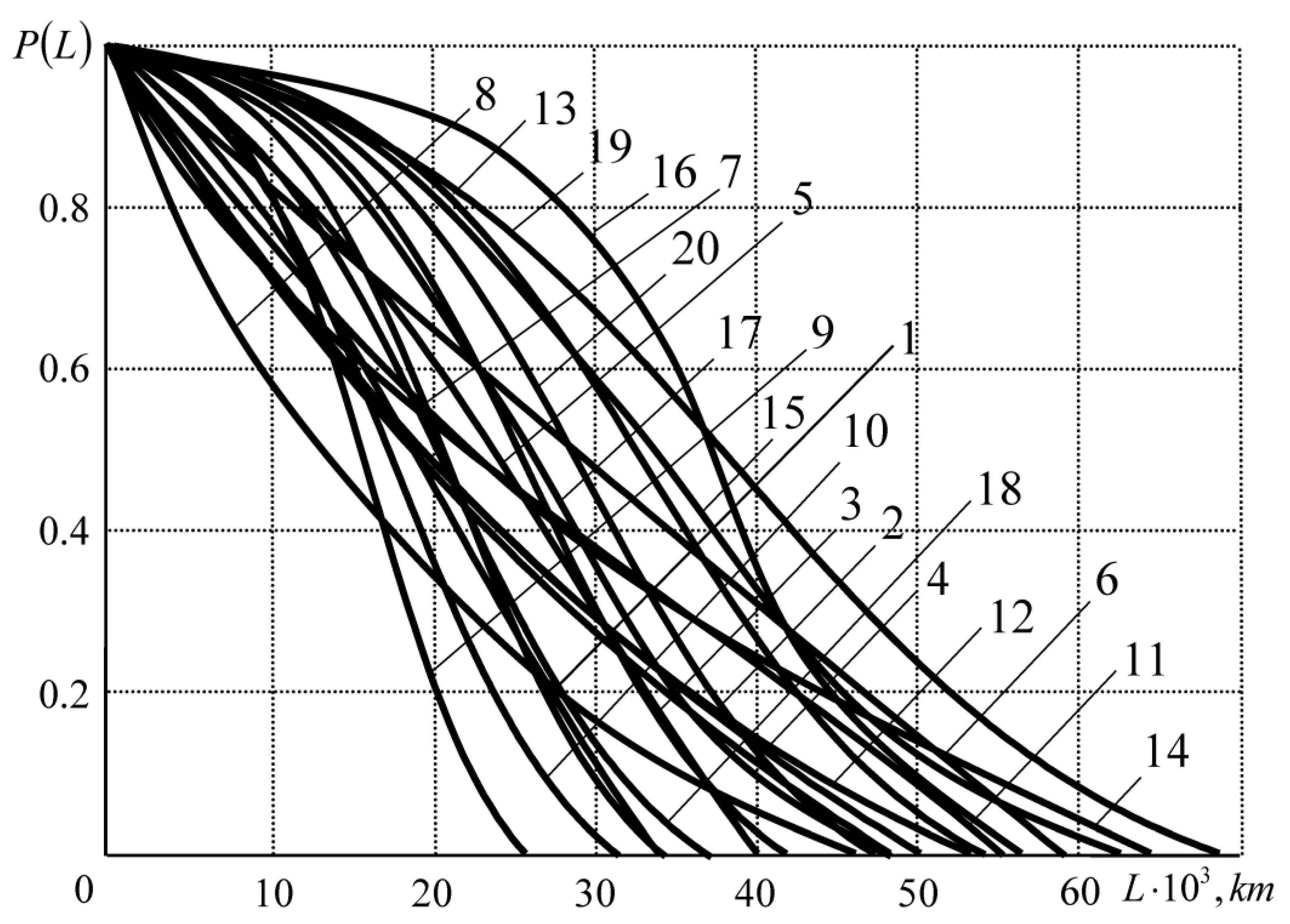
To select the smoothing functions of the obtained empirical curves of the probability of no-failure operation depending on the mileage, analytical software components were developed, i.e., a software module for smooth function interpolation through the median method.

As a result of the interpolation by means of the programs developed by the authors and an analysis of the functions’ convergence, a universal analytical function was selected. The use of this function enables the data obtained from the results of the experiments to be smoothed. Hence, the characteristics of failure-free operation and failures, $P\left(L\right)$, for each type of electrical equipment in electric transport under study were obtained. The methodology that enables the smoothing function for one individual node to be selected is shown in Figure 2. The methodology for all other types of the trolleybus EE is presented in Figure 3. The universal analytical function has the following form:

$$\psi \left(L\right)=\frac{{\xi }_1-{\xi }_2}{1+e^{\frac{\left(L-L_0\right)}{\Delta L}}}+{\xi }_2$$

(3)

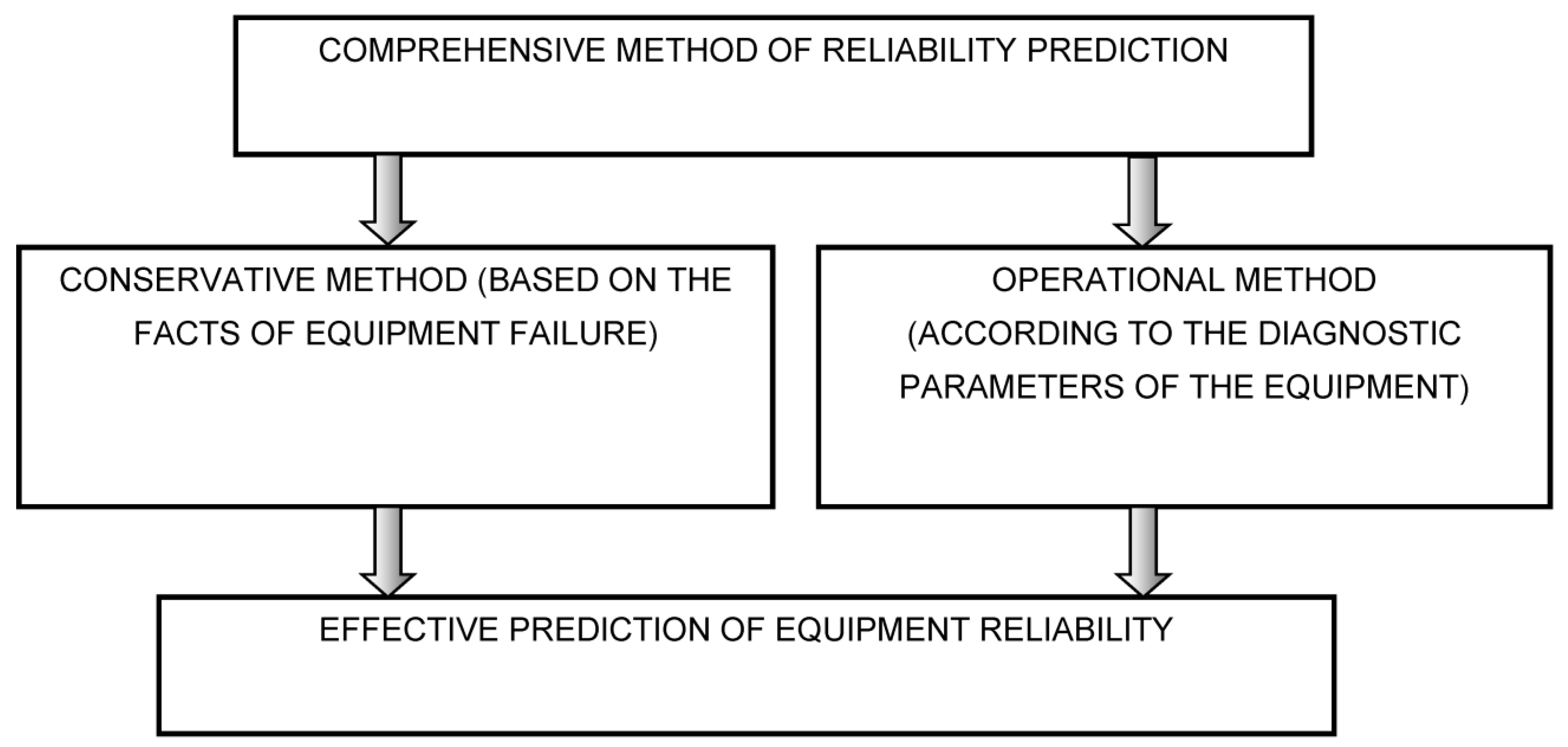
2.3. Comprehensive Method of Reliability Prediction

Known probabilistic stochastic approaches to assessing the technical condition and the prediction of trolleybus electrical equipment serviceability, being low-cost in terms of the funds invested in the technical equipment of operating enterprises [37,38], enable monitoring and making reliability forecasts only in the case of an average statistical unit. Therefore, as a result of the research, a complex method of assessing and predicting serviceability is proposed, which, for the first time, is based on the principle of the homogeneity of changes in the diagnostic parameters [39]. The complex method consists of using two methods: conservative and operational (Figure 4):

• The conservative method determines reliability by means of stochastic models of statistical modeling (according to the facts of equipment failure).
• The operational method enables the equipment’s reliability to be determined using the diagnostic parameters of the equipment.

In spite of the fact that the operational method implies the availability of diagnostic tools in the form of diagnostic benches, rolling lines, and onboard devices (which requires tangible but necessary investments), technical resource monitoring and its prediction can be performed for each individual unit, each EE unit, when determining the reliability of each trolleybus [40].

A continuous evaluation of reliability in the case of each individual unit consists of the following. A set of diagnosable parameters is determined based on the available diagnostic tools and the possibility of determining the intervals of permissible changes in the diagnosed parameter. Then, the diagnostics and numerical determination of the values of the selected diagnostic parameters are performed. After this, the probability of the no-failure operation of the equipment unit according to the given diagnostic parameter is determined [41].

Then, in the presence of the known probabilities, $p\left(A_i\right)$, for several joint events, $A_1, A_2, \dots ,\hspace{0.17em}{A}_i, \dots ,\hspace{0.17em}{A}_n$, a complex event, $A$, consisting of the simultaneous realization of several events, is expressed by the product of the original events, $A_i$:

$$A=A_1·A_2·A_3 \dots A_i \dots A_n=\underset{i=1}{\overset{n}{{\displaystyle \Pi }}}{A}_i$$

(4)

where $A_1, A_2, \dots , A_i, \dots ,\hspace{0.17em}{A}_n$ are the joint events and $p\left(A_i\right)$ is the occurrence probability of the $i$-th event.

Using the probability multiplication theorem, according to which the probability of the product of independent events is equal to the product of the probabilities of these events, we can determine the probability, $p\left(A\right)$, of a complex event, $A$ Hence,

$$p\left(A\right)=\underset{i=1}{\overset{n}{{\displaystyle \Pi }}}p\left(A_i\right)$$

(5)

Then, based on the probability multiplication theorem, we define a point in the coordinates $P\left(t\right)$ or $P\left(L\right)$. Each point corresponds to an act of diagnosis, and, accordingly, the more acts of diagnosis performed, the more points will be located on the coordinate plane. This method is applicable both for diagnostic test benches and on-board diagnostics, which enables diagnostics to be carried out continuously in real time and, thus, for curves of the equipment’s technical service life to be obtained. After obtaining the points, an approximating curve is constructed using the software developed by the authors. To define the approximating functions, universal software components were developed and tested, which will be given separately.

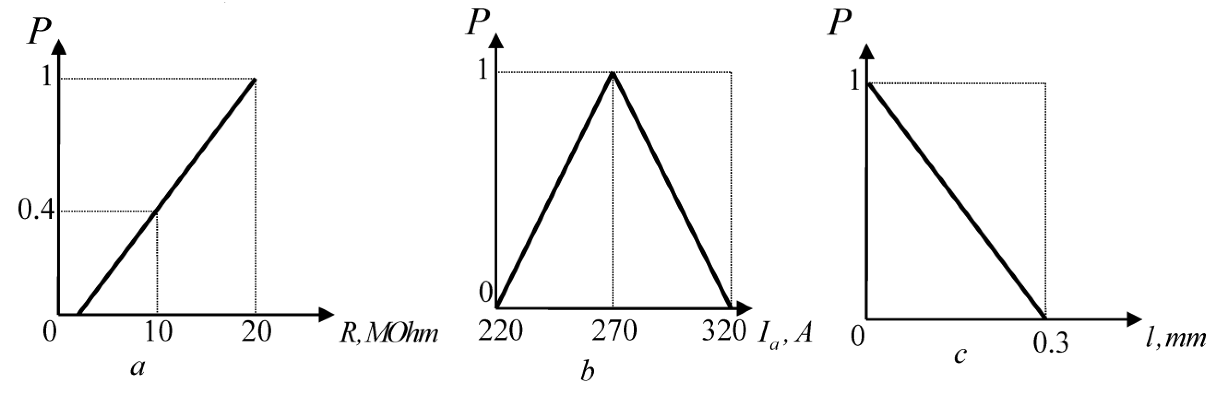
The implementation of the method for determining reliability according to the diagnostic parameters is shown in Figure 5 through the example of a trolleybus electric motor. Three parameters were chosen as diagnostic parameters: the motor insulation resistance, $R$, an armature run out value, $l$, and the traction motor armature current, $I_{motor}$, consumed during start-up. According to (5), we have $P\left(A\right)=f\left(R,\hspace{0.17em}I,\hspace{0.17em}L\right)$, approximated by a linear function. Obtaining the diagnostic parameters through ASCTS, we determine through their quantitative indexes the probability of no-failure operation, first for each of the indexes, and then at the integral level.

3. Results

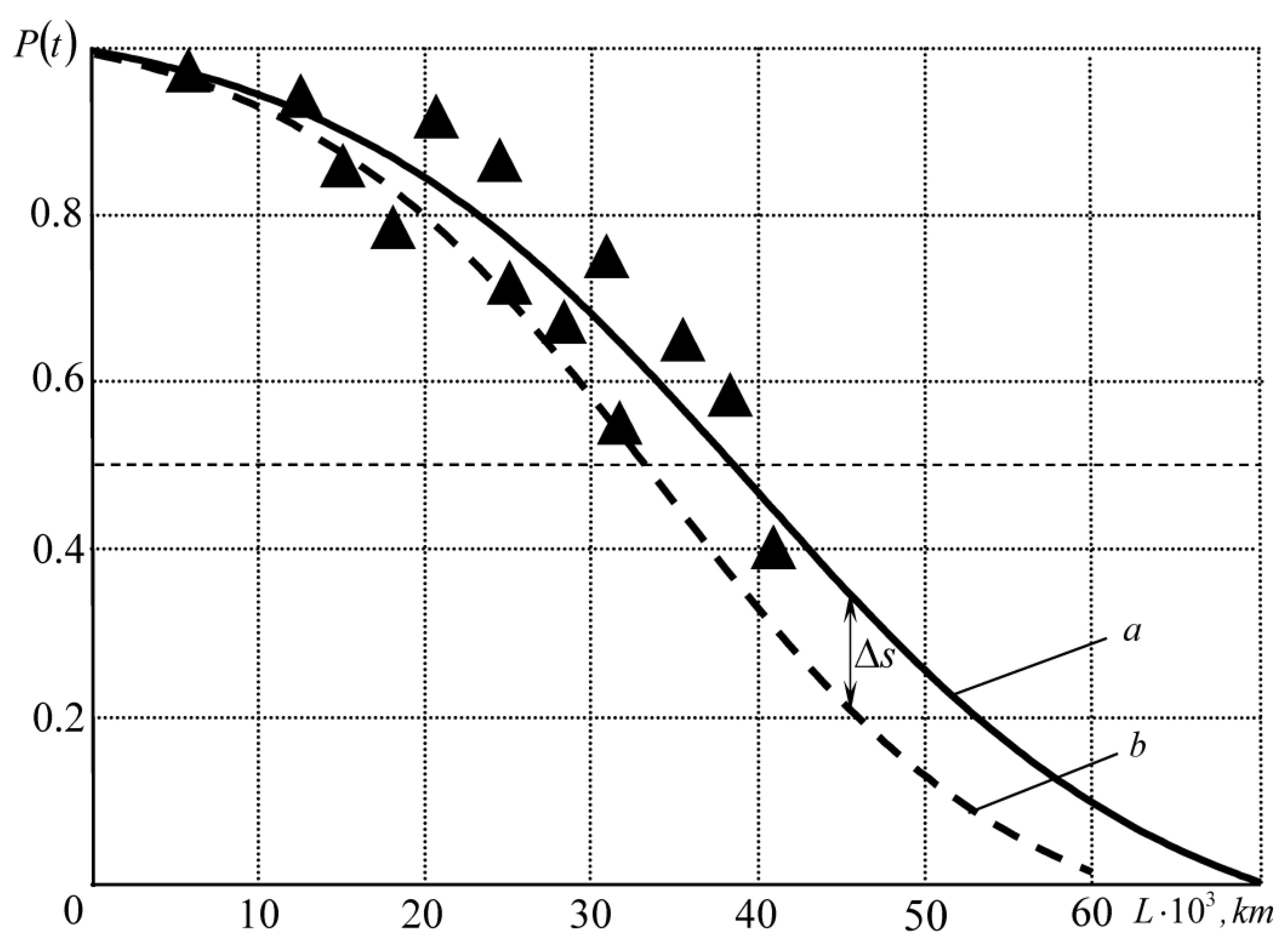
The studies of electrical equipment reliability by means of diagnostic signs showed that the curves obtained through this method pass above the stochastic probability curves, providing, thus, an overestimation of reliability [42]. This can be explained by the fact that the probabilistic stochastic method considers the influence of random factors concerning equipment reliability that change under the operating conditions (Figure 6).

Using the proposed method of researching the trolleybus’ electrical equipment reliability by means of diagnostic signs enables the diagnostic process quality to be assessed by comparing the obtained diagnostic curves with the stochastic ones [43]. The higher the method’s accuracy, the more diagnostic features are used when diagnosing the equipment, and the more accurate the parameters of the diagnostic features are [44,45,46]. Ideally, the value of $\Delta s$ (Figure 6) represents the change in the reliability of the investigated equipment due to external random influences under the operating conditions.

In addition, the method has the properties of self-testing, because if the correlation of the two curves a and b (Figure 6)grows with an increase in the diagnostic parameters, we can say that the signs and diagnostic parameters that extend the diagnostic system have been chosen correctly. Otherwise, it is necessary to discuss the opposite.

This enables the newly proposed diagnostic features and the methods for determining their parameters to be indirectly tested, and the values (or intervals of change) of the parameters to be directly tested.

The optimization of the maintenance system of the electrical complex from the point of view of reliability, first, should be economically justified if catastrophes and human losses are not considered. An economically justified level of reliability is the main criterion for forming an EE trolleybus maintenance system [47].

Since EPS reliability is the most important indicator in the management of vehicle traffic, more and more attention is now being paid to the selection of a certain level of reliability and the implementation of reliability programs during the EPS operation, especially in the case of the dominant use of PSAs.

Since the risk of vehicle failures means a reduction in transportation efficiency reduction, the determination of the required level of EE reliability is based on technical and economic calculations. Insufficient EE reliability in operation leads to great material damage and sometimes irreparable consequences. Economically, the effect of improving the EE reliability is manifested in an increase in the useful operating time of the EE and a reduction in the need for rolling stock, materials, energy, etc.

To select the optimal reliability levels to organize maintenance and repairs of the trolleybus EE, it is necessary to select optimization criteria and the target function.

The target function of the problem of EPS operation at the required level of reliability under modern economic market conditions is the dependence of the annual present costs, $C$, on the sought structure and parameters of the system, and the economic criterion is the minimum of these costs (the so-called method of the present costs) [5].

$$C=a·CI+AC\to \min$$

(6)

where $CI$ is the capital investment; $AC$ is the annual cost; and $a$ is the gearing factor.

In this case, the dynamic target function is reduced to a static form using the discounting procedure of the gearing factor, $a$:

$$a=\frac{1}{{(1+r)}^{-1}+{(1+r)}^{-2}+....+{(1+r)}^{-t}}$$

(7)

where $r$ is the discount rate, which can be a real interest on the capital, and $t$ is the number of the current period of costs.

Implementing measures to improve reliability requires additional labor and money. The EE operation will be more expensive if its reliability is higher. The analysis shows that the operation cost increases faster than the reliability. On the other hand, a more reliable trolleybus is cheaper to operate because the costs to keep it operational are lower. Therefore, there is an optimal level of reliability at which the costs are minimized.

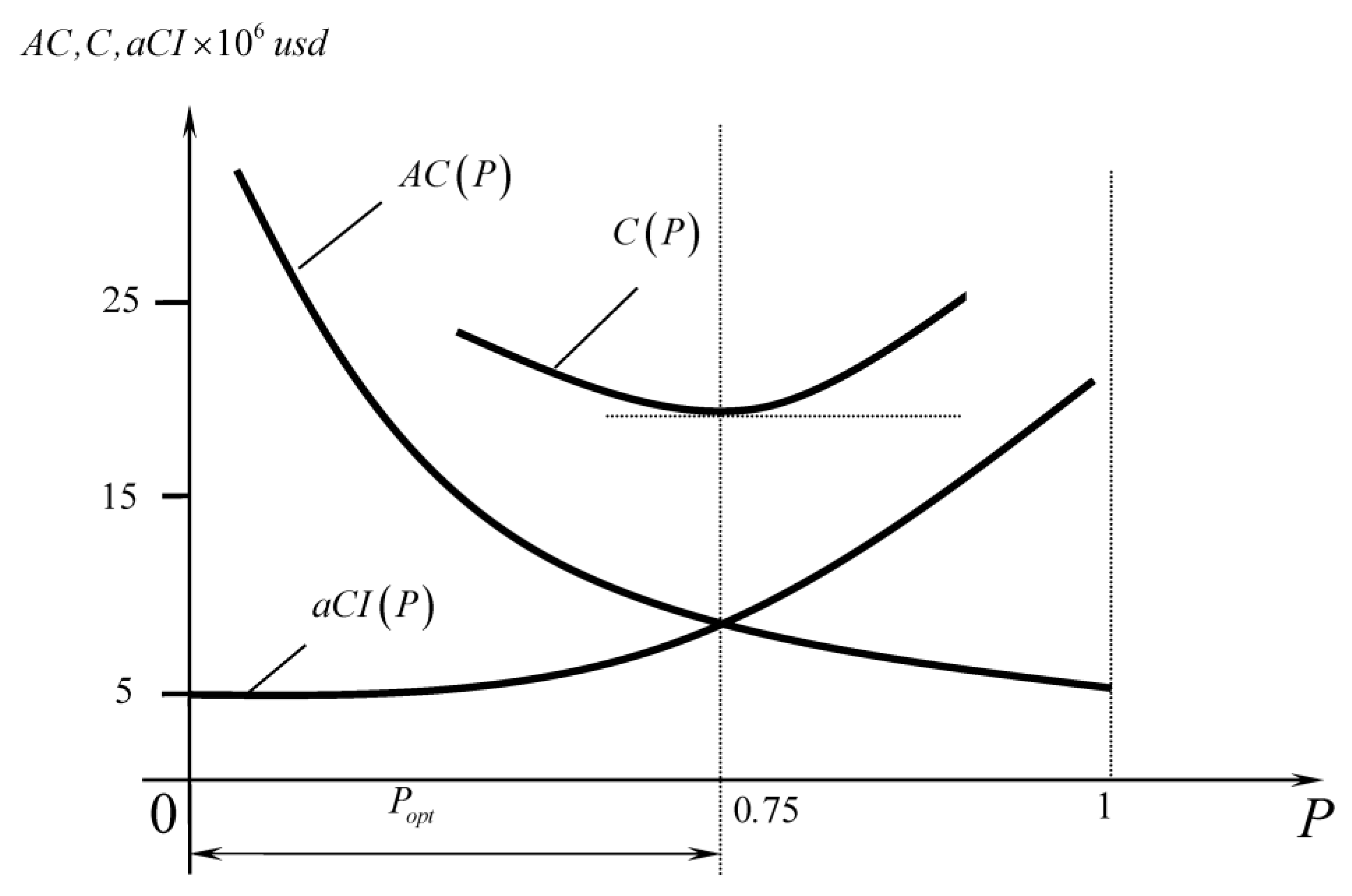
Let us present the dependencies of the present capital investment on the reliability function, $P$, in the form of $aCI(P)$; the operating costs’ dependence on reliability is $AC(P)$, and the present costs’ dependence on reliability is $C(C)$ Then,

$$C(P)=aCI(P)+AC(P)$$

(8)

where $a$ is the discounted reduction factor. The condition for determining the economically optimal level of reliability can be represented as:

$$\frac{dC(P)}{dP}=\frac{d[aCI(P)+AC(P)]}{dP}=0$$

(9)

The root of this equation gives an optimal (economically feasible) value of reliability, $P_{opt}$, as represented in Figure 7 in the case of the EE of 100 trolleybuses during 11 TO-2 (service).

The requirements for the reliability indicators cannot be assigned arbitrarily. They must be determined by the economic value and responsibility of EE units and assemblies. For example, absolute reliability should not be sought for those trolleybus components whose failure does not affect traffic safety. The level of such assemblies should be assigned according to the minimum of the reduced costs, as shown above. On the contrary, trolleybus EE components that ensure traffic safety [12], such as starting and braking rheostats, the accumulator battery, and traffic control systems, should have almost absolute reliability [14].

At the same time, $aCI\left(P\right)$ includes costs for improving the diagnostics process (in some electric transport enterprises, they are practically absent) to modernize the diagnostic equipment and increase the scope, depth, and quality of the diagnostic process. $AC\left(P\right)$ includes the reduction in the costs for unscheduled trolleybus EE repairs due to the reduction in failures during operation because of high-quality tracking diagnostics and the reduction in the costs for trolleybus EE maintenance and repair due to the increase in interrepair periods.

An optimal solution for the trolleybus EE operation is the fact that a given production effect (annual traffic volume, rolling stock use, reliability and quality level, maintenance, and repair costs) is obtained at minimum costs for material and labor resources.

Determining the reliability and predicting the serviceability of the trolleybus electrical complex undoubtedly have a great applied aspect, consisting of a reduction in the maintenance and repair costs of the equipment according to the needs and technical conditions [46,47].

As a result of selecting the trolleybus EE maintenance strategy, to practically use this method to determine the frequency of maintenance of the trolleybus electrical complex based on the failure-free operation probability, acceptable levels of failure-free operation for all of the electrical complex elements were proposed.

An acceptable reliability level of any EE was proposed to be $P\left(L\right)$, which guarantees the trouble-free operation of this element until the next type of maintenance, taking into account the actually achieved reliability level, assessed by the operating time until failure. In the case of the trolleybus and its equipment, there are currently no standards for the failure-free operation probability. Establishing such norms on the basis of the accumulated knowledge obtained from the analysis of the quantitative and qualitative characteristics of operational reliability indicators and based on the suggested methodology of reliability optimization enables four levels of no-failure operation to be accepted. They are acceptable for determining the maintenance intervals and gamma-percent resource. Each of these levels refers to certain elements of the trolleybus electrical complex, whose failures may occur owing to their nature and the following consequences:

-

The trolleybus is not equipped with a safety device (brake contactors, brake rheostats, an electric motor for the power steering pump). For these components, the value of $P\left(L\right)$ must be within the range of 0.95–0.98;

-

The elements (a traction motor, power collectors, power collector heads, a group rheostat controller, a control controller, a circuit breaker, a generator, an auxiliary motor, a door drive motor, a thyristor-pulse control system, contactors, and relays) cause trolleybus returns, causing a large amount of repair work, long downtime, and significant costs. In the case of these elements, the value $P\left(L\right)$ should not be lower than 0.9;

-

Failures are detected and eliminated during maintenance and repair beyond the scope of work specified in the regulations and do not cause the failure of the trolleybus as a whole during the periods between repairs (battery). In the case of such elements of the trolleybus electrical equipment, $P\left(L\right)$ can be 0.8;

-

Failures allow temporary operation of the trolleybus even in case of a failure in lighting, a loudspeaker, a heating stove). For such elements, the value $P\left(L\right)$ should not be lower than 0.3–0.7.

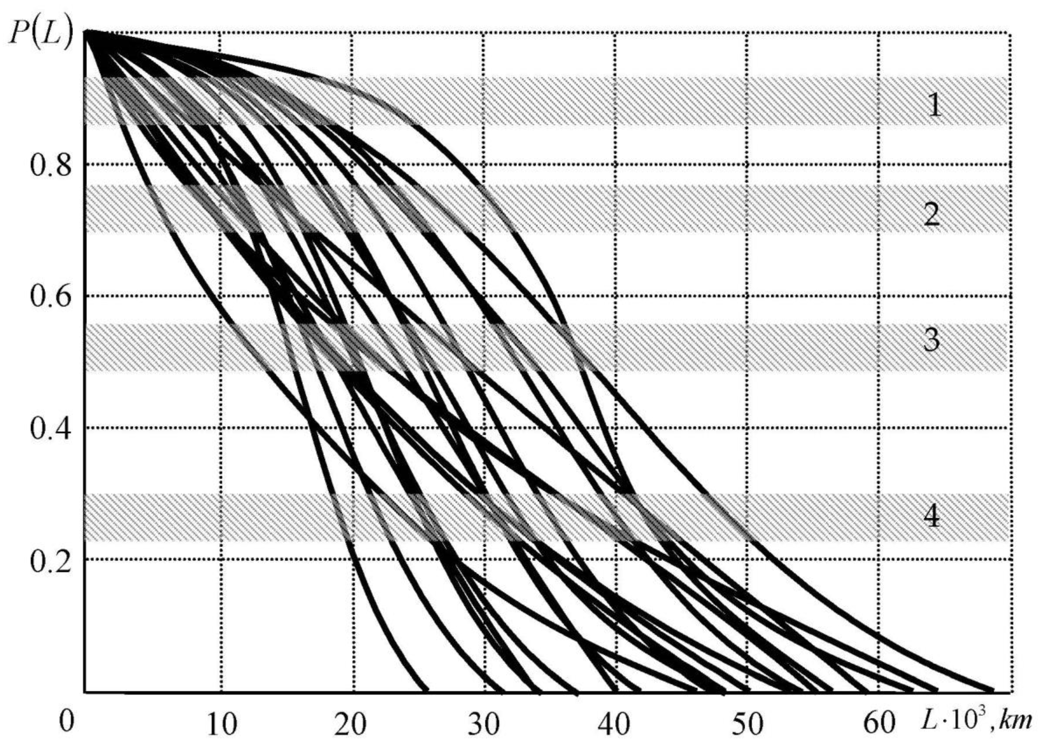
Determining the number of repairs and composing the groups of equipment types can be carried out using the laws of change in the probability of failure-free EE operation according to certain indicators, $P\left(L\right)$. Figure 8 shows the laws of variation in EE reliability and a service area of $1÷4$, in which the equipment should be repaired according to the above proposed ranking. In view of this, setting the required probability of the no-failure operation of the equipment, taking into account the technical and economic resources of the depot, enables maintenance and repair terms after a certain mileage or operating time to be determined. That is, it contributes to making individual schedules for the maintenance and repair of each trolleybus unit containing an individual set of EE elements diagnosed and maintained in the scope of maintenance and repair.

Therefore, combining the types of electrical equipment into groups with approximately the same remaining technical resource, $P\left(L\right)$, enables rational repair–maintenance cycles to be formed, as is carried out in the existing systems of maintenance and repair, for example, in the PSRR, but based on the demand or technical conditions. This means moving to the PSA.

For the economic evaluation of the trolleybus’ electrical equipment’s reliability improvement and the diagnostic complex implementation, a method was developed that considers the costs of the creation and operation of the trolleybus electrical equipment. Its use showed the dependence of specific operating costs on the reliability of the electrical equipment. The study shows that increasing the electrical equipment’s reliability reduces specific capital investments and specific operating costs. Specific capital expenditures are reduced due to the increase in trolleybus productivity during the operation year. There is a reduction in the non-working time intended for maintenance, repair, and failure recovery.

The most important problem that needs to be solved when operating electric transport and trolleybuses in particular is improving the quality of passenger service. At the same time, an equally important problem that requires constant new solutions is reducing operating and repair costs. As a rule, it is extremely difficult to solve the first task and the second task simultaneously. As the service quality growth leads to a growth in costs, it is possible to solve these two problems simultaneously in passenger transportation by optimizing the level of service quality, according to [14]. The study proposes introducing a certain optimality criterion. The minimum of the total transportation costs is taken as such a criterion.

These problems also arise during the electrical equipment’s operation. Mathematical models have been developed to solve the problem of increasing the reliability of the electrical equipment’s operation. These models describe such parameters of the electric equipment for electric transportation as:

$E_c$—The dependence of creation costs on reliability indicators;

$E_e$—The dependence of operating costs on reliability indicators;

$E_p$—The dependence of repair costs on reliability indicators.

There are two ways to improve the reliability of electric transport equipment. The first is by optimizing the reliability level as a whole. And the second is by optimizing the reliability of individual elements along with the subsequent determination of structural reliability as a whole.

Let us consider the first approach, applying it to the reliability of electric transportation (the trolleybus). Using this approach, the cost of a trolleybus with improved reliability, $E_{c1}$, will be defined as:

$$E_{c1}=E\left(E_{c0},\hspace{0.17em}{R}_0,\hspace{0.17em}{R}_1\right)$$

(10)

where $E_{c0}$ is the cost of the electric transport having the initial (basic) reliability level and $R_0,\hspace{0.17em}{R}_1$ are the levels of electric vehicle reliability. This level is measured quantitatively both before (R₀) and after (R₁) the reliability improvements.

Since the cost of building a trolleybus also depends on its power, in Equation (10), $E_c$ is understood as the unit cost per unit of power. The function $E\left(E_{c0},\hspace{0.17em}{R}_0,\hspace{0.17em}{R}_1\right)$ should have the following properties:

• $E\left(E_{c0},\hspace{0.17em}{R}_0,\hspace{0.17em}{R}_1\right)>0$, since the costs are non-negative values;
• $E\left(E_{c0},\hspace{0.17em}{R}_0,\hspace{0.17em}{R}_1\right)>E_{c0}$;
• $\underset{H_{1\to 1}}{\lim }E\left(E_{c0},\hspace{0.17em}{R}_0,\hspace{0.17em}{R}_1\right)=\infty$, which results from the fact that absolute reliability cannot be obtained in real-world design and manufacturing operations;
• $E\left(E_{c0},\hspace{0.17em}{R}_0,\hspace{0.17em}{R}_1\right)\le E\left(E_{c0},\hspace{0.17em}{R}_0,\hspace{0.17em}{R}_2\right)$ if $R_1<R_2$ and $E\left(E_{c0},\hspace{0.17em}{R}_0,\hspace{0.17em}{R}_1\right)\ge E\left(E_{c0},\hspace{0.17em}R{\prime }_0^{},\hspace{0.17em}{R}_1\right)$ if $R_0<R{\prime }_0$; that is, $E\left(E_{c0},\hspace{0.17em}{R}_0,\hspace{0.17em}{R}_1\right)k$ does not decrease by $R_1$ when $R_0$ is fixed and does not increase by $R_0$ when $R_1$ is fixed. This is because an increase in reliability may be associated with additional costs.

Formula (10) uses a composite indicator to evaluate the $R$ reliability level. This complex indicator reflects most of the reliability components. They include maintainability, durability, and failure-free operation. Various coefficients often act as such an indicator. These can be coefficients of technical utilization, $K_{tu}$, and downtime, $K_{dt}$. They depend on both uptime and recovery time.

For Formula (10), its properties, 1 $÷$ 4, will be satisfied by an exponential function of the form:

$$f\left(x\right)=k·x^a$$

(11)

Then, we have:

$$E_{c1}=E_{c0}·{\left(\frac{1-K_{tu0}}{1-K_{tu1}}\right)}^a=E_{co}{\left(\frac{K_{dt0}}{K_{dt1}}\right)}^a$$

(12)

where $K_{tu0},\hspace{0.17em}{K}_{dt0}$ are the coefficients of technical utilization and trolleybus downtime before implementing reliability improvements;

$K_{tu1},\hspace{0.17em}{K}_{dt1}$ are the coefficients of technical utilization and downtime of electric transport after the implementation of reliability improvements;

$\alpha$ is a statistical coefficient. This coefficient shows the extent to which reliability characteristics increase as a function of the investment made to improve them.

The statistical coefficient, $\alpha$, is calculated as the mathematical expectation of the known laws of a random variable distribution for the electric transport node used. In the subsequent stages, it will be calculated using the statistical observation data after taking certain measures.

The expenses occurring during the period of operation, $t$, for trolleybus repair and maintenance will be as follows:

$$E_{mr}=E_m+E_r$$

(13)

where $E_m$ are the maintenance costs of a trolleybus in good working condition and $E_r$ are the repair costs of a trolleybus.

Expressing $E_m$ and $E_r$ through the unit costs, $e_m$ and $e_r$, per unit time of the trolleybus in good and bad conditions, respectively:

$$E_m=e_m·K_{tu}·t=e_m·\left(1-K_{dt}\right)·t$$

(14)

$$E_r=e_r·\left(1-K_{tu}\right)·t=e_r·K_{dt}·t$$

(15)

Provided that the costs of repairs in the process of use are formed at the moment $t$, it is necessary to bring them to the initial moment, that is, to the time of creation. Instead of the discrete method of reduction using the normative coefficient $E_{norm}$, we will apply the method of continuous reduction. Then, the maintenance costs can be represented as:

$$E_m^{red}=e_m·\left(1-K_{dt}\right)·\frac{1}{\gamma }·\left[1-\exp \left(1-\gamma ·t\right)\right]=e_m·\left(1-K_{dt}\right)·t_{red}$$

(16)

where $\gamma =\frac{1}{8760}·\ln \left(1+E_{norm}\right)$.

$t_{red}$ is the conditional time that takes into account bringing the costs to the starting point. This time is calculated by the formula:

$$t_{red}=\frac{1}{\gamma }·\left[1-\exp \left(-\gamma ·t\right)\right]$$

(17)

For the second component of Formula (18), provided that (12) will be similar,

$$E_r^{red}=e_r·K_{dt}·t_{red}$$

(18)

The total costs can be calculated taking into account the diagnostic complex according to Equation (12) $÷$ (15). On this basis, the total costs of creating and operating electric transport (the trolleybus) with increased reliability can be calculated as:

$$\begin{array}{l}{E}_{\Sigma 1}=E_{c0}·{\left(\frac{K_{dt0}}{K_{dt1}}\right)}^{\alpha }+E_m^{red}+E_r^{red}=E_{c0}·{\left(\frac{K_{dt0}}{K_{dt1}}\right)}^{\alpha }+e_m·\left(1-K_{dt1}\right)·t_{red}+\\ +e_r·K_{dt1}·t_{red}\end{array}$$

(19)

Based on (19), let us determine the fact that, when $\frac{d{E}_{\Sigma 1}}{d{K}_{dt1}}=0$, the minimum value of $E_{\Sigma 1}^{\min }$ corresponds to the optimal level of reliability:

$$K_{dt}^{opt}={\left[\frac{\alpha ·E_{c0}}{\left(e_n-e_{mo}\right)·t_{red}}\right]}^{\frac{1}{\alpha +1}}·K_{dt0}^{\frac{\alpha }{\alpha +1_{}}}$$

(20)

Using Equation (20), we can calculate the optimal level of reliability of one unit of electric transportation. This level of reliability will be characterized by the idle ratio, $K_{dt1}^{opt}$, or technical utilization ratio, $K_{tu1}^{opt}=1-K_{dt1}^{opt}$. Using Formula (19), we can calculate the total costs, $E_{\Sigma 1}^{\min }$, and the economic effect gained due to increasing the reliability of electric transport up to the optimal level. The calculation is made for one unit of electric transport:

$$EcE{f}_{or}=E_{\Sigma 0}-E_{\Sigma 1}^{\min }$$

(21)

The reliability of the electrical equipment in the process of its operation is characterized by its durability, failure-free operation, and maintainability. The overall economic effect, $EcE{f}_{er}$, of the reliability improvement is composed of a number of individual economic effects. $EcE{f}_{er}$ includes three parameters: an increase in the $EcE{f}_f$ effect owing to an increase in fail-safety, the $EcE{f}_d$ effect due to an increase in durability, and the $EcE{f}_m$ effect gained because of the increase in maintainability. At the same time, these economic effects do not take into account the costs of improving the reliability of electric transport (the trolleybus):

$$EcE{f}_{er}={\left[\left(EcE{f}_f+EcE{f}_d+EcE{f}_m\right)-E_{norm}·K\right]}^{}·N, \mathrm{USD}/\mathrm{year}$$

(22)

where $E_{norm}$ is the normative payback ratio;

$K$ is the one-time cost for improving the reliability of electric vehicles;

$N$ is the number of electric vehicles (trolleybuses) in operation.

The economic effect obtained within the year as a result of the increase in the trolleybus’ operating time can be determined as follows:

$$EcE{f}_f=\frac{L_{an1}}{L_{av1}}·D_1-\frac{L_{an2}}{L_{av2}}·D_2+\frac{\Delta t_{troll}·E_{norm}·P{r}_{troll}}{8760}, \mathrm{USD}/\mathrm{year}$$

(23)

where $L_{an1}$ and $L_{an2}$ are the trolleybus annual mileages before and after the safety improvement, in km; $L_{av1}$ and $L_{av2}$ are the trolleybus uptimes, characterized by the average operating time per failure before and after the safety improvement, in km/failure; $D_1$ and $D_2$ are the damages caused by a trolleybus failure before and after the safety improvement, in RUB/failure; $P{r}_{troll}$ is the trolleybus price; 8760 is the annual fund for working hours, h; $\Delta t_{troll}$ is the time saving as a result of trolleybus electrical equipment failure-free operation. The time saving is defined as:

$$\Delta t_{troll}=\frac{L_{an1}}{L_{av1}}·{\tau }_{dt1}-\frac{L_{an2}}{L_{av2}}·{\tau }_{dt2}, \mathrm{USD}/\mathrm{year}$$

(24)

where, ${\tau }_{dt1}$ and ${\tau }_{dt2}$ are the average downtimes of the electric transport (trolleybus). That is, this is the time of being in repair due to a failure occurrence. ${\tau }_{dt1}$ is the time before increasing the uptime, in h. ${\tau }_{dt2}$ is the time after increasing the uptime, in h.

The annual economic effect gained from the increase in the durability of the trolleybus used in this work is calculated according to the formula:

$$\begin{array}{l}EcE{f}_d=\underset{i=1}{\overset{k_p}{\Sigma }}\left(\frac{L_{an1}}{L_{pi1}}·c_{i1}-\frac{L_{an2}}{L_{pi2}}·c_{i2}\right)+\underset{i=1}{\overset{k_p}{\Sigma }}\left(\frac{L_{an1}}{L_{pi1}}·{\tau }_{i1}·c_m-\frac{L_{an2}}{L_{pi2}}·{\tau }_{i2}·c_m\right)+\\ +\underset{i=1}{\overset{k_p}{\Sigma }}\frac{\Delta {\tau }_{mi}}{8760}·E_{norm}·P{r}_{troll}\end{array}$$

(25)

where $L_{pi1}$ and $L_{pi2}$ are the total mileages of the used trolleybus determined between different $i$ (types of repairs). $L_{pi1}$ is the mileage before the durability improvement, in km, and $L_{pi2}$ is the mileage after the durability improvement, in km;

$c_{i1}$ and $c_{i2}$ are the costs of the $i$-type of trolleybus repair. $c_{i1}$ is the cost before the durability improvement, in RUB. $c_{i2}$ is the cost after the durability improvement, in RUB.

${\tau }_{i1}$ and ${\tau }_{i2}$ are the durations of the electric transport downtime for the $i$-type of repair. ${\tau }_{i1}$ is the downtime before the durability improvement, in h and ${\tau }_{i2}$ is the downtime after the durability improvement, in h.

$c_{dt}$ is the cost of one hour of downtime for electric vehicles under repair, in RUB;

$\Delta {\tau }_{mi}$ is the number of working hours saved for electric transport in the $i$-type of repair. The savings are obtained as a result of the increased durability and uptime of electric vehicles.

Expression (25) is intended for calculating only the repairs, the mileages between which have changed. Moreover, this change occurred as a result of the durability increase. The increase in durability should be determined while taking into account the cyclic coefficient.

The economic effect gained per year by increasing the maintainability of the trolleybus is calculated by the formula:

$$EcE{f}_m=\frac{L_{an1}}{L_{av1}}·{\tau }_{dt1}·c_{dt}-\frac{L_{an2}}{L_{av2}}·{\tau }_{dt2}·c_{dt}$$

(26)

We will calculate the payback period of one-time costs, $K$, designed and used to improve the reliability of the used electrical equipment of the trolleybus as follows:

$$T_{pb}=\frac{K}{EcE{f}_f+EcE{f}_d+EcE{f}_m}$$

(27)

Using the presented formulas, we obtain the payback period of the diagnostic system proposed in this paper, which is $T_{pb}=1.6$ years.

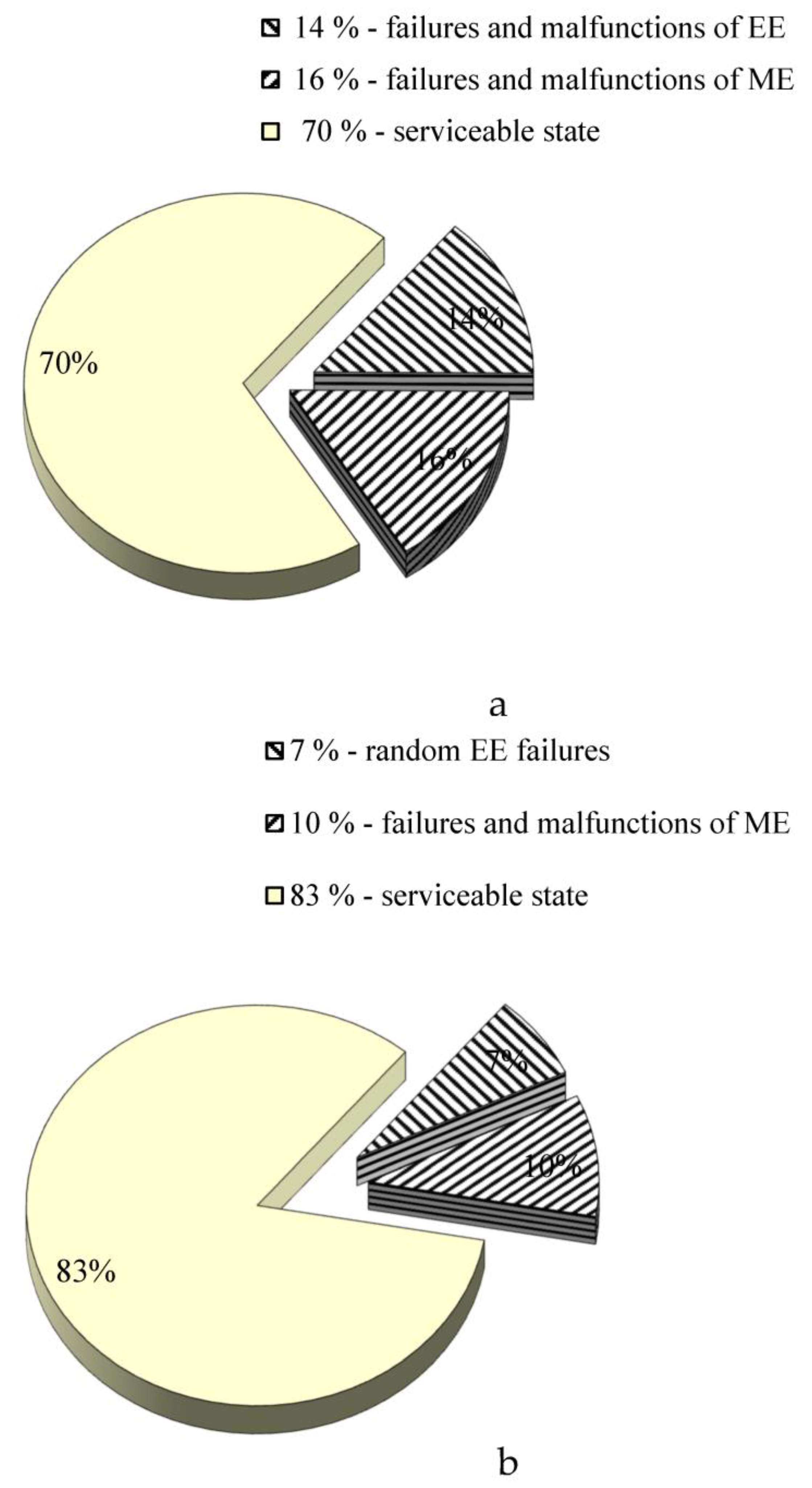
The analysis of the failure statistics of the used electric transport equipment at the enterprise where the proposed system was implemented showed a decrease in the number of failures. Within a year, the total number of failures of the electric transport equipment decreased from 30% to 17% on average (Figure 9). Moreover, the reduction in the failures of electrical equipment was two times, and the number of mechanical equipment failures decreased by 60%. This is an indirect confirmation of the fact that the serviceability and failure-free operation of mechanical equipment depend on the serviceability of electrical equipment. The remaining 7% were accidental failures. The accidental failures in our case depended on external operational factors.

4. Discussion

The presented approach, based on a reliability assessment and serviceability forecasting of urban electric buses proceeding from a newly proposed scientific method of complex reliability assessment and forecasting, enables the rolling stock diagnostics to be connected and their reliability to be determined, considering the conservative component of the reliability determination from equipment failures and the operational component from the diagnostic equipment parameters of the EE. In this paper, a unique complex method, the essence of which we will explain below, is used to solve the problems of reliability assessment and performance prediction of urban electric buses and electric coaches.

The known probabilistic stochastic approaches to assessing the technical condition and forecasting the serviceability of the electrical equipment of trolleybuses and electric buses, being low-cost from the point of view of their organization, allow for monitoring and making reliability forecasts only for an average unit. Therefore, as a result of the research, a complex method of performance evaluation and prognosis was proposed, which is based on the principle of the homogeneity of changes in the diagnostic parameters for the first time. The complex method consists of two components: a conservative component and an operational component.

• The conservative component involves the determination of reliability using stochastic models of statistical modeling (from information on equipment failure). This is a traditional method, noted, for example, in modern publications [48].
• The operational component enables the equipment reliability to be determined using diagnostic EE parameters. The uniqueness of this component consists of the fact that the authors, for the first time, proposed an algorithm to mathematically and technically realize the transition from diagnostic attributes and equipment parameters directly to reliability parameters in numerical form. This approach was successfully tested and verified experimentally, as mentioned in this work.

Despite the fact that the operational method assumes the availability of diagnostic means in the form of diagnostic benches, rolling lines, and on-board devices (requiring tangible but sufficient capital investments), the technical resource can be monitored and forecasted for each separate unit, i.e., each electrical equipment node, when determining the reliability of each electric bus, but not for an average of many electric buses. This is particularly important.

A continuous reliability assessment of each individual unit consists of the following. A set of diagnosed parameters is determined based on the available means of diagnostics and the possibility of determining the intervals of permissible changes in the diagnosed parameter. Then, the diagnostics and a numerical determination of the values of the selected diagnostic parameters are carried out. Then, the probability of the failure-free operation of the equipment unit is determined for a specific diagnostic parameter (Figure 5).

The two approaches are combined by comparing the two curves of the integrated method with each other (Figure 6), and the magnitude of the scatter between them provides information about truly random failures that cannot be influenced. In view of this, it is possible to clearly determine the proportion of random factors affecting the technical condition of electric buses. This is also the novelty of the method. The operational component of the method is self-adjusting, and it enables the degree of the real influence of the selected diagnosable parameters on the electric bus’s reliability to be determined. This is also the uniqueness of the proposed method. The modeling results are adequate and can be confirmed by the experimental data of the real operating depot. So, after using the results of the presented mathematical model and the new method, the number of reliable equipment units increased and the number of equipment failures decreased by 13%, which is a significant increase in reliability. Such a reliability level enables significant financial resources of the depot to be freed up for self-development by reducing random failures and, as a consequence, the cost of them.

The new proposed method of equipment reliability improvement, based on the joint use of two methods, provides completely new perspectives that are based not on a qualitative but on a quantitative evaluation of a resource, which can be processed and evaluated using computational means. But it is rather difficult to make such a combination due to the underdevelopment of the approaches and the mathematical component of the theory of diagnostics.

The batteries on an autonomous trolleybus are used in the city of Novosibirsk. The length of one leg of the run is 20 km. Therefore, a trolleybus can travel about 40 km without connecting current collectors to current-carrying wires. After connecting to the current-carrying wires, the batteries have time to charge for 40 min up to a 100% charge level. The reliability of lithium-ion batteries is provided by two units installed on the trolleybus rolling stock. If one battery fails, the second battery is capable of autonomous movement within 10 km in one direction or 20 km in total, which is quite sufficient under the city’s conditions in areas that are not equipped with a contact network.

Autonomous trolleybuses have only been actively developed in the last decade. Therefore, there is not much data on the failure statistics of their operation. They have appeared in mass amounts only in the last 10–15 years. In order to show any significant results, we need statistics for at least 3–5 years of operation. Therefore, the work performed in the field of electric transport reliability is very relevant. In our paper, we have presented a study on the operation and reliability of already known and brand new vehicles; these are trolleybuses and electric buses, which are highly demanded systems. The presented method of determining and improving reliability enables the advantages and disadvantages of both types of rolling stock to be compared in operation.

Proceeding from the proposed complex method of diagnosing and determining electrical equipment reliability using the maximum likelihood method, a modeling method based on the selection of a universal alignment function for a set of types of electrical equipment of the electric bus is proposed.

The results of this study are in line with the results of other studies conducted in different countries of the world [48,49]. Determining the current technical life of the EE of a trolleybus and forecasting it for the future in terms of the average of elements and individual elements reveals great opportunities for optimizing repair and maintenance systems, which results in an overall reduction in operating costs.

5. Conclusions

• The testability of the electrical equipment of trolleybuses and electric buses has been assessed, which determines the adaptability of EE to diagnostic works, providing, under certain conditions, the necessary reliability for the minimum labor, time, and cost. The equipment testability assessment is especially important for older vehicle models that do not have intelligent information interfaces and built-in diagnostic sensors.
• An approach has been developed that determines the damage degree of electrical equipment elements by means of a statistical analysis. This approach is extremely important in assessing the overall reliability of the electrical complex of electric transportation as a whole.
• The mathematical expectation of mileage is proposed as a numerical characteristic of a statistical series of failures of electrical equipment, and in estimating the relative characteristic of electrical equipment reliability, it serves as the main component of its reliability. In this case, determining the relative characteristic of electrical equipment reliability is proposed through the indicator characterizing the number of equipment failures per unit mileage, i.e., through the failure flow.
• As a result of the analysis of the existing methods of modeling the electrical equipment state on the basis of the maximum likelihood method, a modeling method based on the selection of a universal alignment function for a set of trolleybus electrical equipment types is proposed.
• This paper presents a probabilistic–diagnostic system of forecasting and monitoring. This system is designed to continuously monitor the complex electrical state of electric transport, enabling the operability of the used electrical equipment to be forecast. The system has been tested in operation at transportation enterprises. The approbation showed that the system reduced the number of electric bus equipment failures by 13% and significantly reduced the cost of liquidating the consequences of emergency failures.
• As a result of the conducted research, the complex method of estimating and forecasting serviceability is synthesized, which is based on the principle of the homogeneity of change occurring in diagnostic parameters for the first time. The method consists of two components: a conservative component and an operational component. The conservative component determined reliability using stochastic models of statistical modeling (based on knowledge of equipment failure). The operative component means the equipment reliability determination using the diagnostic parameters of the equipment.
• Probability norms for the failure-free operation of electrical equipment, which have not been available so far, are proposed. The maintenance system of the electrical equipment of trolleybuses is optimized on the basis of the system of forecasting the technical condition at the level of equipment reliability.
• A methodology for the economic evaluation of trolleybus electrical equipment reliability improvement is developed, which enables the costs of the electrical equipment’s creation and operation to be determined.
• Analyzing the collected statistics on the failures of trolleybus electrical equipment after applying the technical condition prediction system confirms the fact that the number of failures decreased from 30% to 17% on average. And the total number of failures and malfunctions decreased by almost two times. In view of this, the presented method of monitoring and improving the reliability of operating electric transport can be recommended for all transportation enterprises.

Conclusions 1, 7, and 8 are recommended, first of all, for trolleybus designers and equipment manufacturers; conclusions 2–6 and 9 will be interesting, first of all, for operating enterprises and depots, as well as repair organizations that carry out maintenance and repairs of trolleybuses.