Abstract
Wireless power transfer (WPT) chargers are promising solutions for charging electric vehicles (EVs). Due to their advantages such as ease and safety of use, these chargers are increasingly replacing conductive ones. In this paper, we first provide a detailed analysis to illustrate the effect of varying parameters on the operation of the WPT charger. Secondly, we present the main design steps of the charger elements while respecting the recommendations of the SAEJ2954 standard in terms of operating frequency, efficiency and misalignments. Regarding the design of the ground-side and vehicle-side coils, we propose three different circular geometries whose parameters are determined using an iterative approach. The latter is compared with a finite element analysis performed under Ansys Maxwell software showing the convergence between theoretical calculations and the simulation results. Finally, an experimental prototype with a power of 500 W is realized. In addition, different test scenarios are performed to validate the proposed design approach. In this respect, an efficiency of 90% is obtained for a power of 500 W and a distance between coils of 125 mm. Moreover, the test of the charger in the most unfavorable operating case (misalignments of Δx = 70 mm, Δy = 10 mm and Δz = 150 mm) gives an efficiency of 83.5%, which remains above the limit of the SAEJ2954 standard.
1. Introduction
As is well known, EVs and HEVs are equipped with a rechargeable battery pack providing the power needed to propel the vehicle and also to supply other integrated electrical systems. Due to its limited capacity, the battery requires regular charging from a power station. Depending on the way the energy is transmitted from the Electric Vehicle Supply Equipment (EVSE) to the EV, one could divide the developed charging solutions into two main categories, namely, wireless power transfer (WPT) chargers and conductive chargers [1,2].
Conductive charging relies on dedicated cables to transfer the power from the EVSE to the vehicle. Thus, depending on the configuration of the latter, the charging operation could be performed either in AC or DC mode [3]. In terms of charging times, DC chargers are commonly known as fast chargers, while AC ones are slow due to their limited power transfer capability [4]. The main disadvantage of conductive charging could be related to the safety and comfort of the user. Indeed, the user must intervene in the charging operation by handling heavy cables. In addition, under certain specific conditions such as snow and rain, the charging operation becomes dangerous and may cause electric shocks [5]. Unlike conductive charging, wireless charging is performed without any contact between the vehicle and the EVSE. Indeed, instead of using cables, the power transfer is performed wirelessly [6,7].
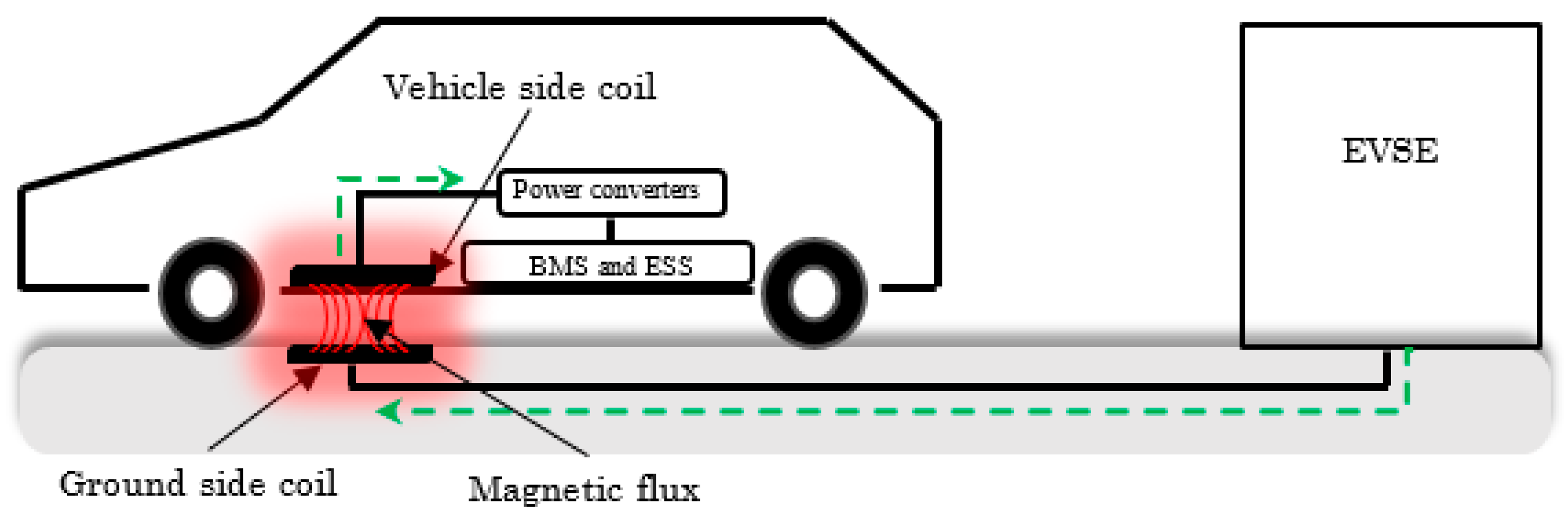
The simplified concept of a static WPT charging system is shown in Figure 1. It is divided into two subsystems: a vehicle assembly (VA) and a ground assembly (GA). The power is wirelessly transferred, using the magnetic field (MF), from the emitting coil embedded in the ground to the receiving one installed underneath the vehicle. Regarding safety and ease of use, powering an EV using the wireless method is much easier and safer for the user [8]. In addition, the absence of physical contact (no mechanical friction) can reduce the maintenance of the wireless charger and prolong its lifetime [9,10].
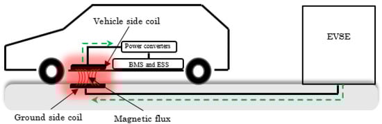
Figure 1.
Simplified concept of a WPT charger.
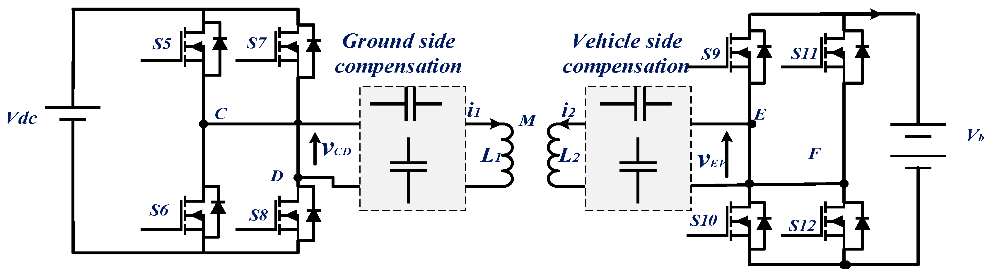
The circuit topology of a WPT charger is shown in Figure 2. The high-frequency inverter, on the ground side, is controlled using phase-shift control technique [11] producing a square wave voltage. This voltage, varying at a frequency of 85 kHz, feeds the ground-side coil. This creates a time-varying magnetic field which, in turn, induces a voltage in the vehicle-side coil due to the mutual coupling between the two coils. The induced voltage is rectified and the resulting DC voltage is used to supply the EV battery [12]. Each of the ground and vehicle-side coils is associated with a reactive energy compensation block. The latter is formed by capacitors connected either in parallel or in series with the coils [13].
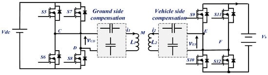
Figure 2.
Circuit topology of a WPT charger.
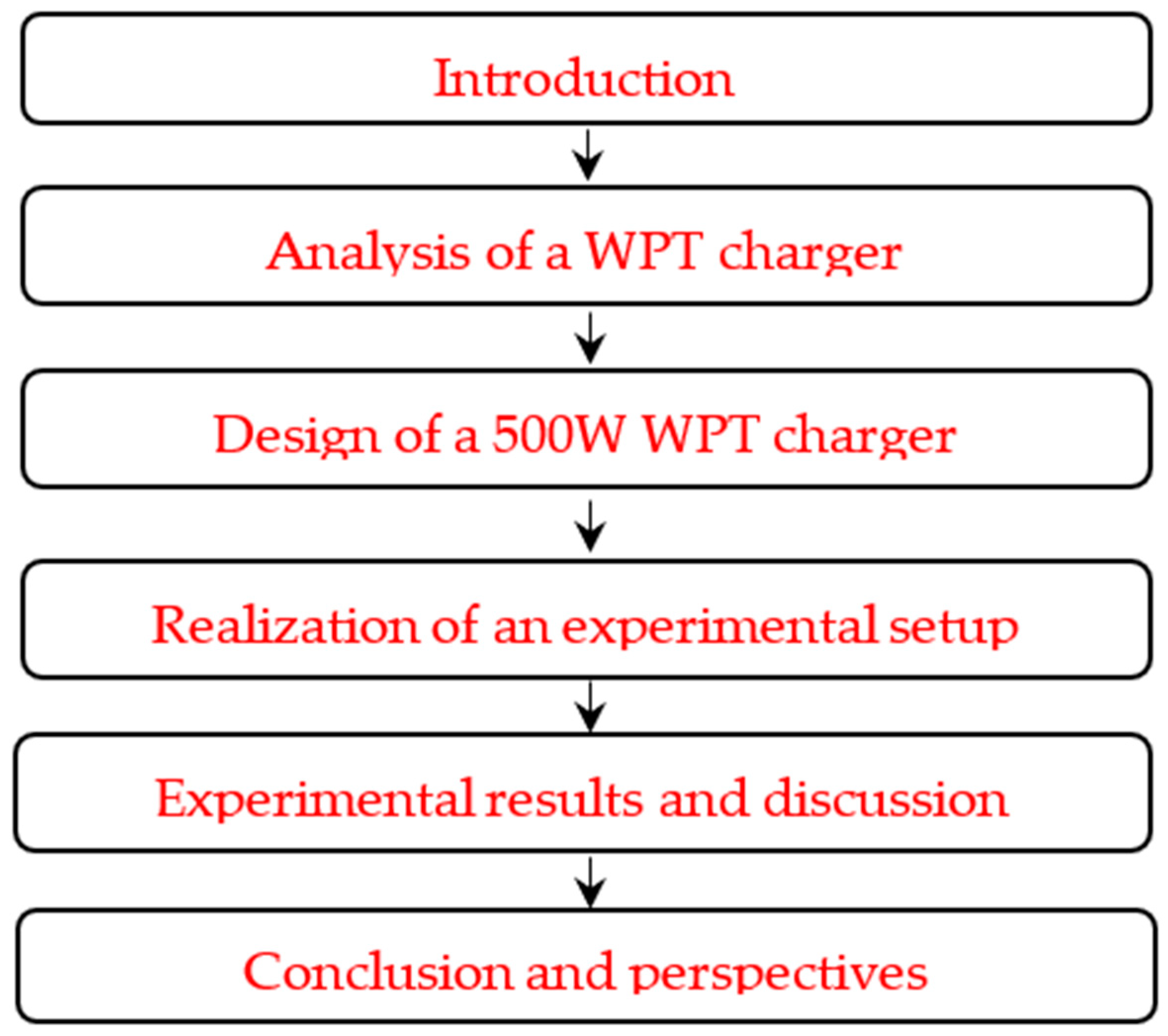
This article deals with WPT chargers from theoretical analysis to experimental realization. Indeed, the article presents a detailed analysis of the main phenomena occurring in a WPT charger. In addition, all elements of the charger, namely, power converters, coils and compensation boards, are designed in accordance with the requirements of the SAEJ2954 standard. Moreover, an experimental setup is realized to verify the effectiveness of the proposed design approach. This article is structured as shown in the following flowchart (Figure 3).
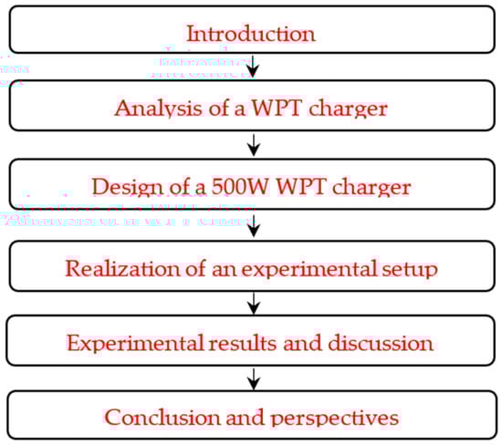
Figure 3.
Flowchart of the organization of the paper.
2. Analysis of Series–Series Compensated WPT Charger
2.1. Effect of the Compensation Network on the Efficiency of the WPT Charger
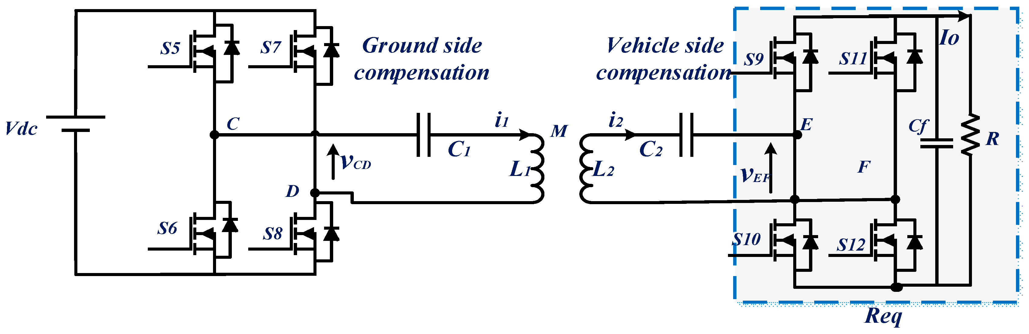
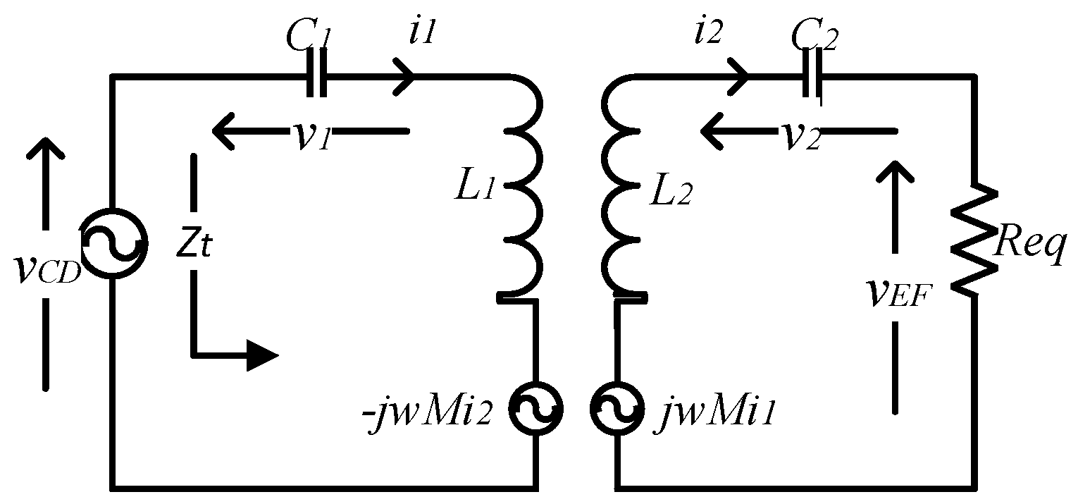
Consider a WPT charger with serial–serial compensation topology, as shown in Figure 4, where the EV’s battery is replaced by a resistive load. In addition, the vehicle-side converter works as a diode rectifier. Thus, assuming that the rectifier is lossless and the current i2 flowing in the vehicle-side coil is sinusoidal, using the power conservation rule, the rectifier, the filtering capacitor Cf and the resistive load R could be replaced by an equivalent resistance Req where the expression is given in (1). In light of all this, an equivalent circuit of a series–series compensated WPT charger is as shown in Figure 5 [14].
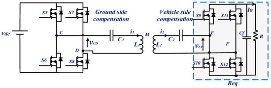
Figure 4.
WPT circuit with serial–serial compensation.

Figure 5.
Equivalent circuit of a WPT system with a serial–serial compensation network.
The total equivalent impedance of the WPT system, seen from the ground side, is given in (2):
where r1 and r2 stand, respectively, for the ground-side and vehicle-side coil’s internal resistances, w is the operating angular frequency (2 * π * 85,000 rad/s) and M is the mutual inductance between the coils.
The power transferred to the load could be expressed as follows:
where I1,RMS is the RMS value of the current in the ground-side coil and I0 is the average value of the load current.
The compensation capacitors are generally calculated in such a way that the ground-side capacitor (C1) cancels out the reactance of the equivalent total impedance (Zt) of the WPT circuit, while the vehicle-side one (C2) maximizes the power transfer (Pout). In other words, C1 and C2 are calculated, respectively, using (4) and (5).
The obtained expressions are given in (6) and (7).
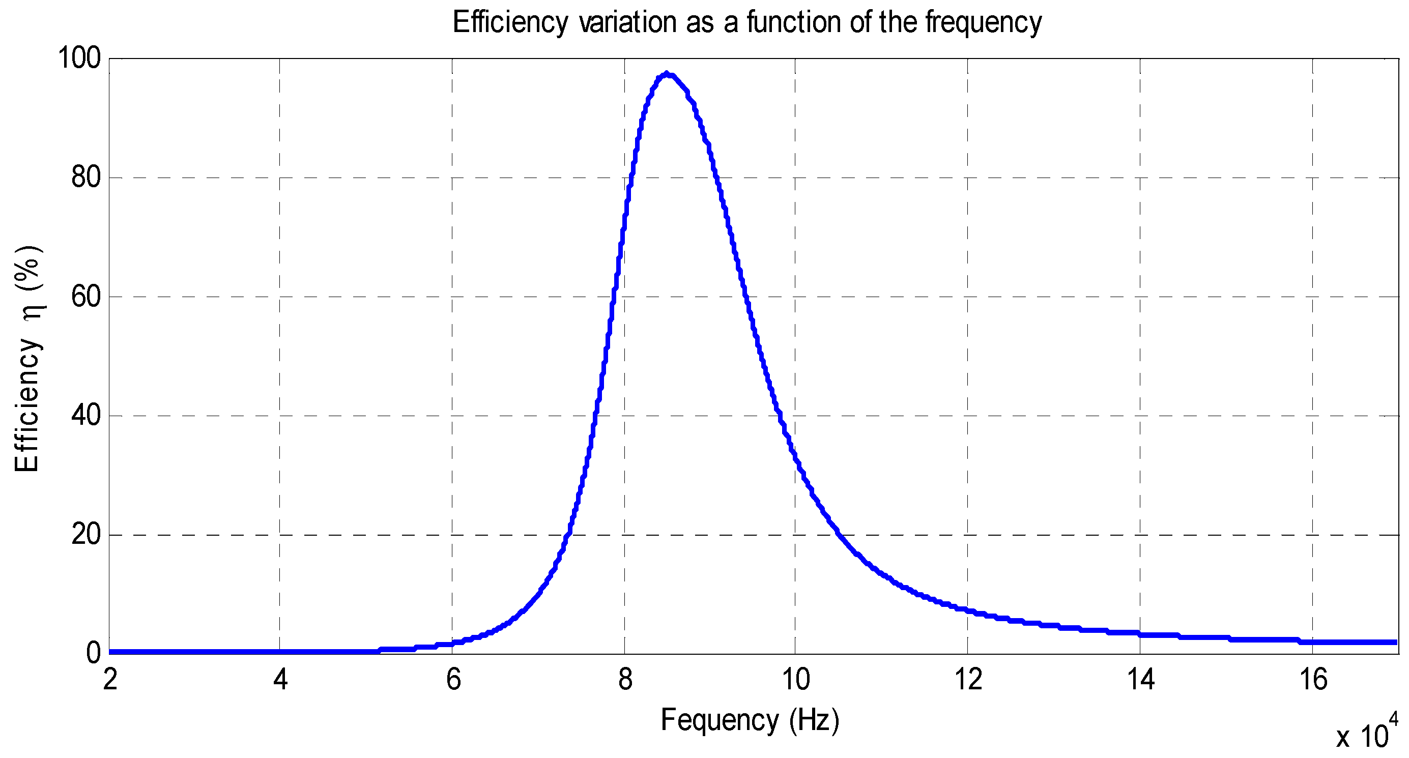
Figure 6 illustrates the evolution of the efficiency of the WPT charger as a function of the frequency. It can be seen that the efficiency reaches its maximum at the resonant frequency, which is 85 kHz. However, when the WPT operates at a frequency other than the resonant frequency, the efficiency drops and tends towards zero.
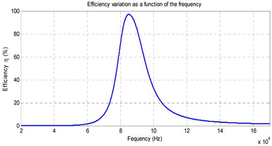
Figure 6.
Efficiency variations of a WPT charger as a function of the frequency.
The peak efficiency is due to the fact that when the capacitors are tuned to the calculated expressions, the overall reactance of the circuit is cancelled and the power transfer capacity is increased. This is well illustrated in (8) and (9).
2.2. Effect of the Coupling Coefficient on the Power Transfer Efficiency
The aim of this subsection is to assess the effect of the coupling coefficient k, defined in (10), on the efficiency of the WPT charger. To note that k is close to unity for a strongly coupled inductor as in transformers, while it decreases in WPT applications due to the large distance and misalignments between the coils.
Assuming the capacitors are properly tuned to ensure the resonance condition, the input power, sent from the ground side, can be expressed as follows:
Using (9) and (11), the power transfer efficiency can be obtained as shown in (12):
Inserting (10) in (12), the relationship between the power transfer efficiency and the coupling coefficient can be obtained as follows:
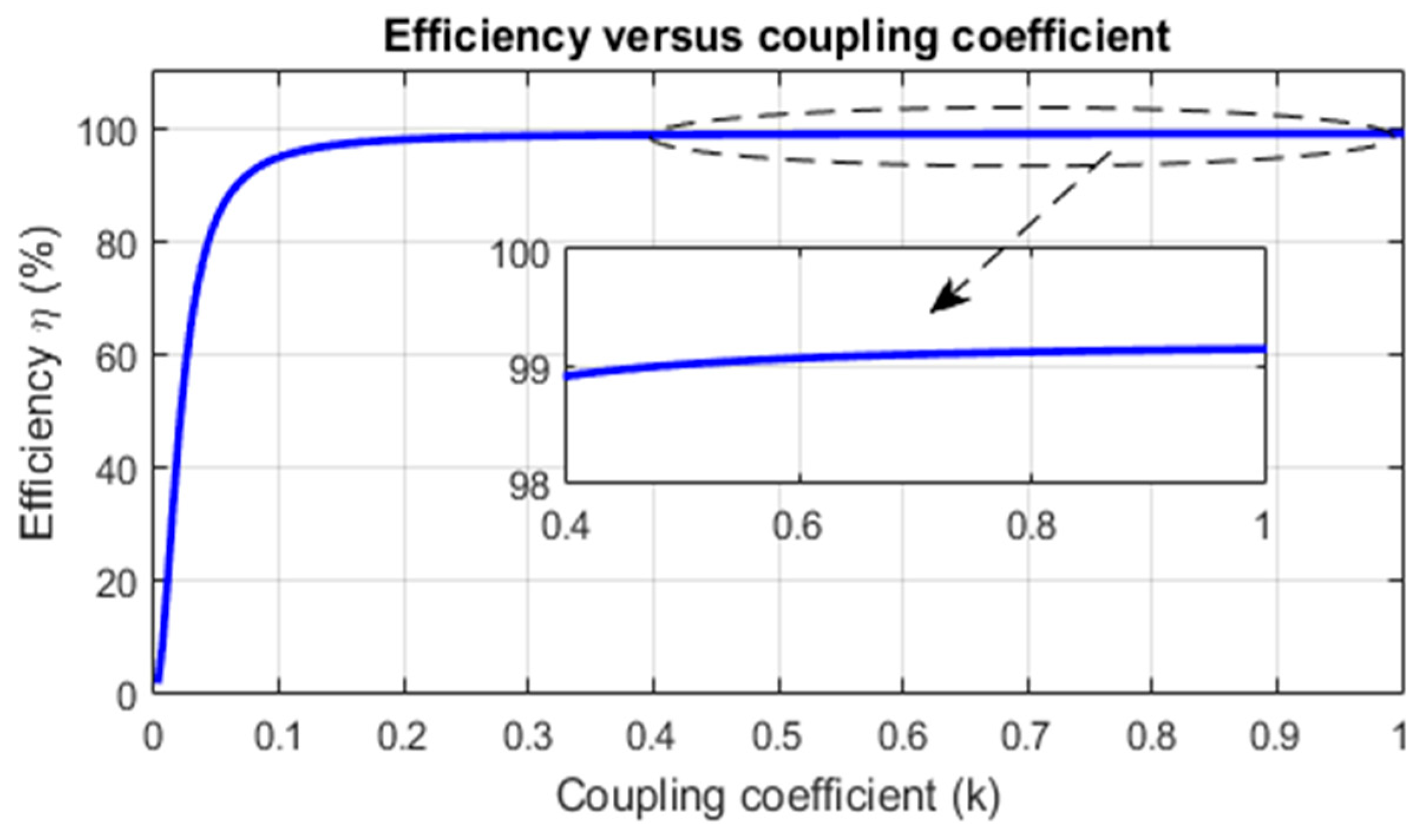
To illustrate the effect of the coupling coefficient on the power transfer efficiency, Equation (13) is plotted in Figure 7 using the parameters listed in Table 1. It can be seen in this figure that the efficiency is strongly affected by the coupling coefficient. Indeed, in the presence of low coupling between the ground-side and vehicle-side coils, which is the most common case in practice, the efficiency drops rapidly. Therefore, at fixed air-gaps between the coils, it is strongly recommended to minimize the misalignments in order to ensure high coupling. In addition, ferrite rods are key components that must be added to the coils in order to enhance the coupling coefficient and, ultimately, the power transfer efficiency.
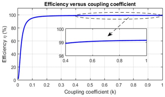
Figure 7.
Efficiency variations of a WPT charger as a function of the coupling coefficient.

Table 1.
Parameters used for plotting Equation (13).
2.3. Bifurcation Phenomenon in a WPT Charger
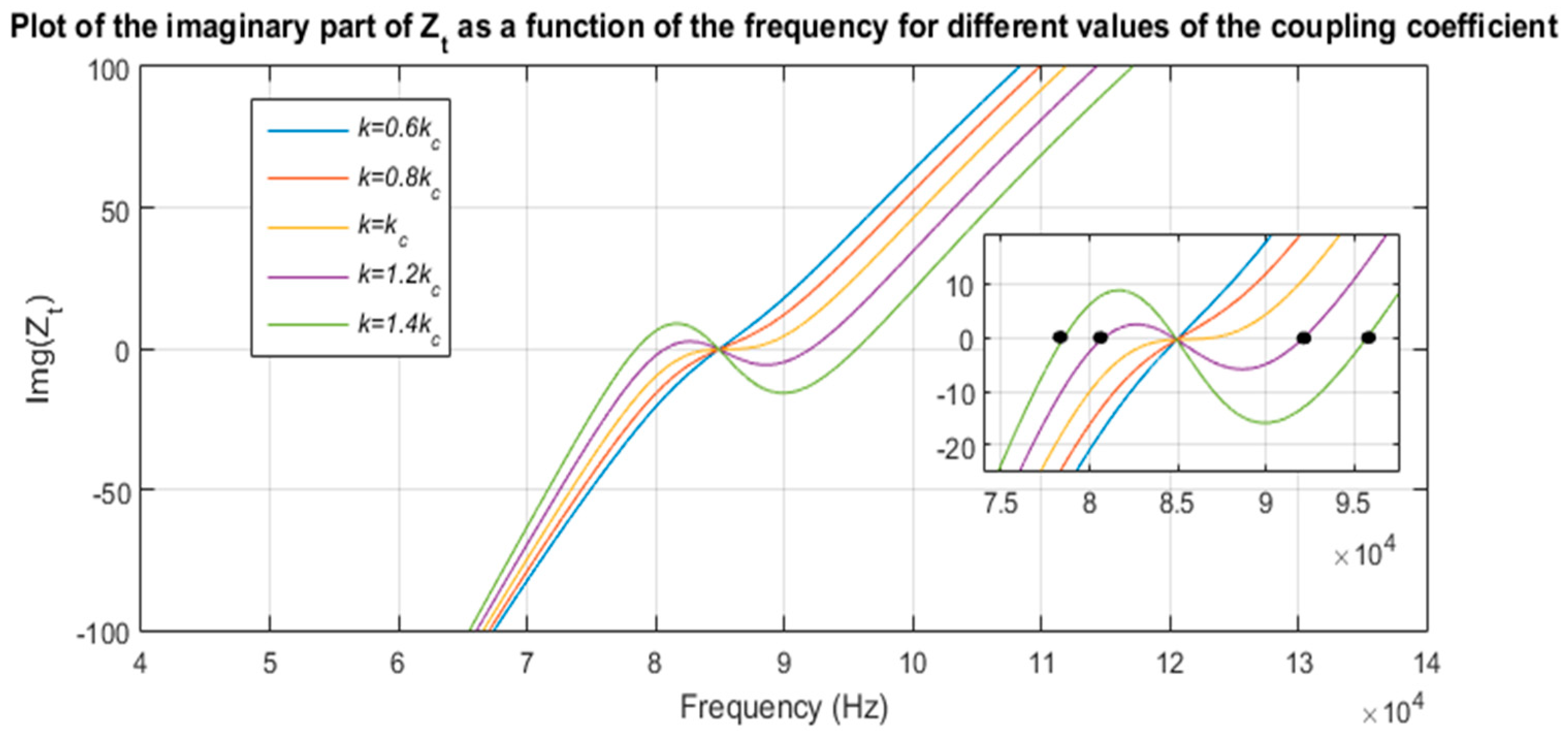
The WPT charger is a double tuned circuit. Thus, a common characteristic of these types of circuits is the bifurcation phenomenon, also known in the literature as frequency splitting [15]. This phenomenon is characterized by the existence of more than one zero-phase angle. In a WPT circuit, this phenomenon appears when the coupling coefficient exceeds a certain limit. It was established in the literature that the bifurcation phenomenon can be avoided if the WPT’s parameters are chosen so that the condition shown in (14) is verified [16].
where is the critical coupling and Q2 is the quality factor of the vehicle-side circuit. The latter is defined as follows:
To illustrate this phenomenon, the imaginary part of the total impedance seen from the ground side (Zt) is plotted as a function of the frequency and for different values of the coupling coefficient. It can be seen in the Figure 8 that when k < kc, only one zero-phase angle exists. However, for k > kc, three zero-phase angles appear.
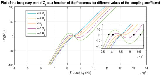
Figure 8.
Evolution of the imaginary part of the impedance seen from the ground side as a function of the frequency for different values of the coupling coefficient and for a fixed load.
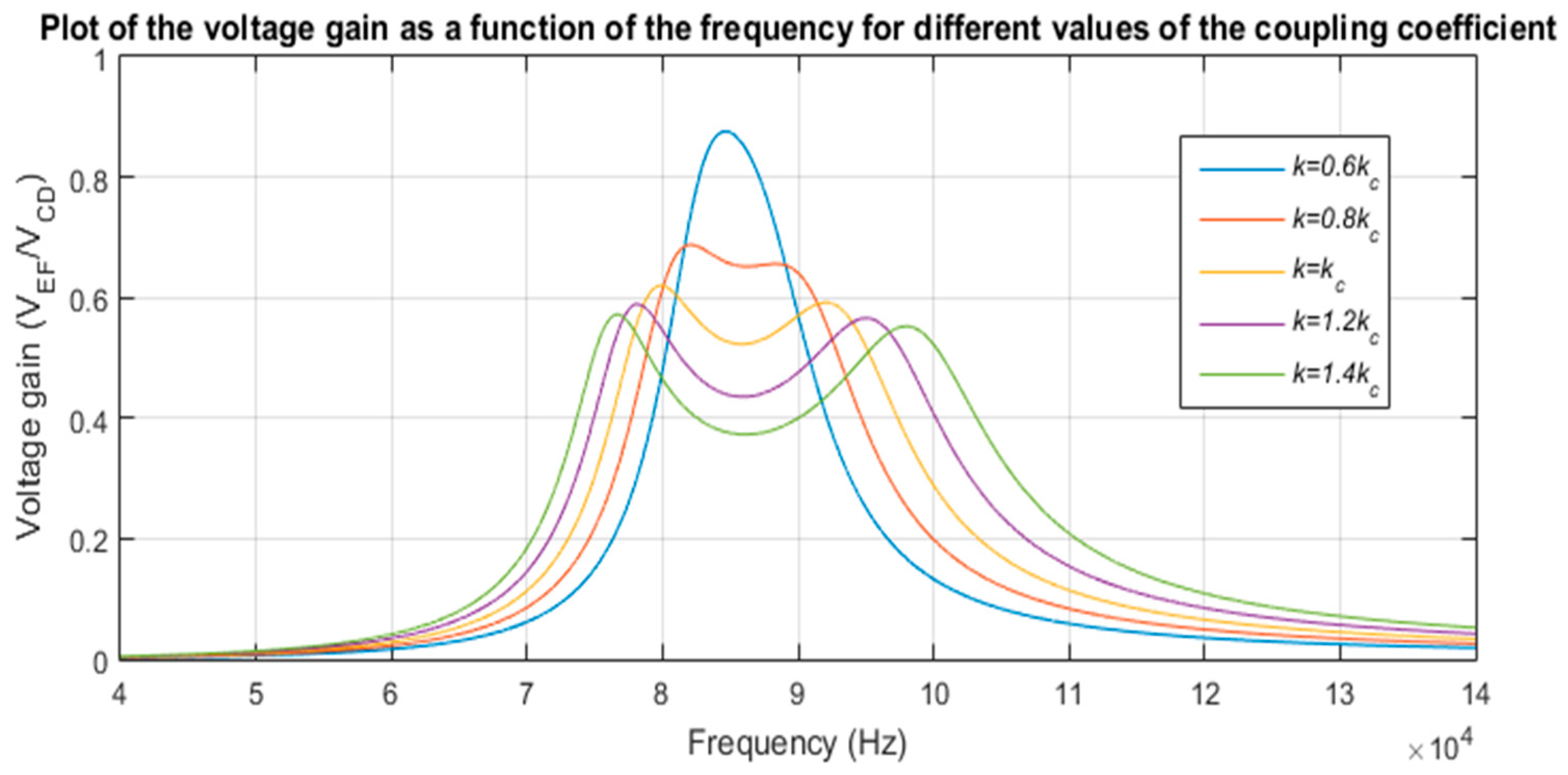
It should be noted that the bifurcation phenomenon strongly affects the power transfer capability and efficiency of the WPT circuit [16]. In this regard, the evolution of the voltage gain (VEF/VCD), for a constant load, as a function of the frequency and for different values of the coupling coefficient is plotted in Figure 9. It can be seen in this figure that when the coupling increases above kc, the voltage gain decreases. This means that a higher current will be needed to transfer the same amount of power to the load.
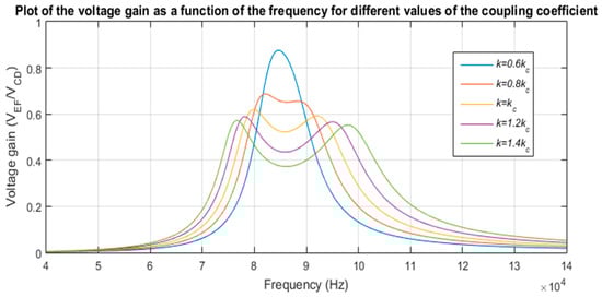
Figure 9.
Evolution of the voltage gain as a function of the frequency for different values of the coupling coefficient and for a fixed load.
2.4. Effect of the Load Variations on the Power Transfer Efficiency
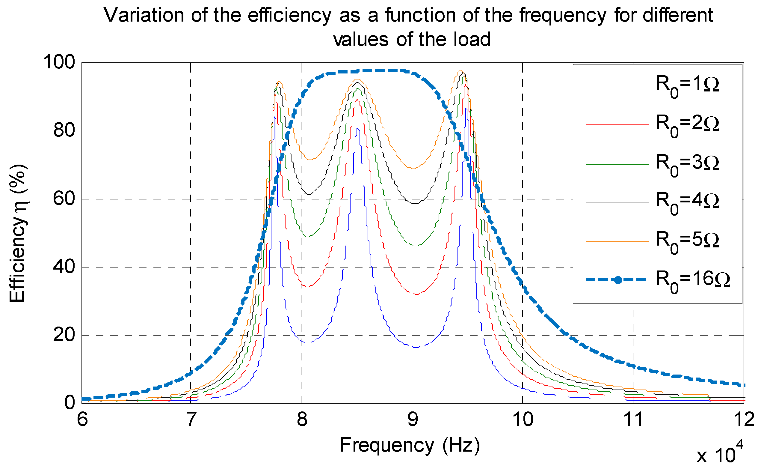
When the coupling coefficient is maintained constant, the variations of the load can also affect the WPT efficiency, as illustrated in Figure 10. It follows that an optimal load ensuring high-power transfer efficiency needs to be expressed. To that end, the derivative of the efficiency with respect to Req is used as in (16):
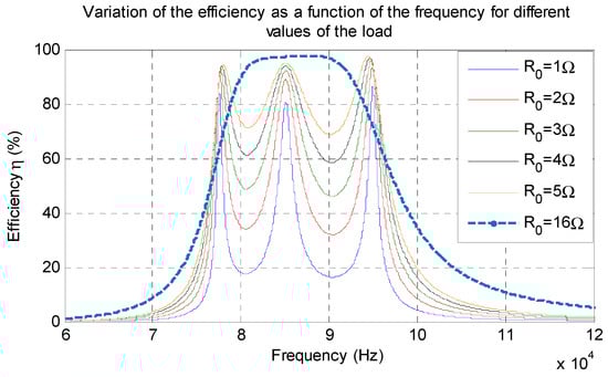
Figure 10.
Evolution of the efficiency as a function of the frequency for different loads.
The optimal load ensuring maximum efficiency is then obtained as follows:
One can notice in the above figure that the efficiency is strongly affected when the load decreases. This is due to the fact that the condition given in (14) is no longer verified. For instance, assume that , and , when the load () decreases the quality factor () increases and the bifurcation-free condition is no longer respected.
In view of this, for a fixed coupling coefficient, the load must verify the condition given in (18) in order to avoid the bifurcation phenomenon.
where .
2.5. Effect of the DC Side and Battery Voltages on the Power Transfer
The aim of this subsection is to analyze the effect of the DC side and battery voltages on the amount of the power transferred to the battery. To simplify the analysis, the coils’ intrinsic resistances r1 and r2 are considered negligible. In addition, the capacitors C1 and C2 are chosen so that:
The current flowing into the ground- and vehicle-side coils could be expressed, respectively, as shown in (20) and (21).
Likewise, the expressions of the ground-side and vehicle-side inverter output voltages vCD and vEF are established using Fourier analysis as shown, respectively, in (22) and (23).
where and are, respectively, the phase-shifts driving the ground-side and vehicle-side inverters, while is the phase shift between the ground-side and vehicle-side inverters’ output voltages.
Neglecting the high-order harmonics, due to the band-pass filtering behavior of the capacitors in series with the coils, only the fundamental components of the inverters’ output voltages and current are considered; it follows that the expression of the fundamental power is obtained as shown in (24).
One can see in (24) that the power flow direction (Grid to Vehicle G2V or Vehicle to Grid V2G) can be controlled by setting for G2V mode and for V2G one. It is also clear that the amount of transferred power can be controlled by adjusting and . It should be noted that only the G2V mode is considered in our case (i.e., and ).
The evolution of the power transfer as a function of the DC side and battery voltages is illustrated in Figure 11. It can be seen that when the mutual coupling is fixed, the transferred power is limited by the voltages on the DC side and battery side. In addition, when the mutual coupling becomes very low (due to large air gaps and misalignments between the coils), the transferred power is expected to exceed the maximal limit. In this case, the phase-shift angles will be adjusted so that the transferred power remains within the maximal power limit of the WPT charger.
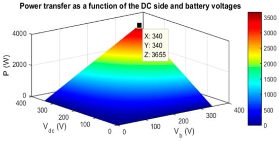
Figure 11.
Evolution of the power transfer as a function of the DC side and battery voltage for a fixed mutual coupling.
3. Design Steps of WPT Charger
The main objective of the present subsection is to highlight the design procedure of a WPT charger, where the specifications are listed in Table 2. The power is scaled down to 500 W since the main objective is to illustrate the main design steps, which remain valid for any other power ranges. It is worth noting that the WPT charger’s parameters are chosen according to the SAEJ2954 standard. Indeed, the operating frequency and the minimum efficiency are set respectively to 85 kHz and 80%. Thus, the air-gap distance between the coils is chosen in the interval 100–150 mm. In addition, the DC side voltage (Vdc) is limited by the available DC power supply in the laboratory. The latter could be adjusted from 0 V to a maximum value of 300 V. Moreover, the battery pack is built by using four 12 V batteries branched in series connection, which leads to a nominal voltage of 48 V.
Table 2.
General specifications of the 500 W WPT laboratory prototype.
Once the power, the DC side voltage and the battery side voltage are fixed, the next step consists of calculating the required mutual inductance, which is necessary for transferring a power of 500 W. To that end, Equation (24) is used as follows:
3.1. Step 1: Choice of Ground- and Vehicle-Side Converter Technology
As the WPT charger is operating at a frequency of 85 kHz, appropriate power converters must be chosen while to minimize the power switching losses. In this regard, the choice is between two emerging technologies, namely, Silicon Carbide MOSFET (SiC-MOSFET) and Gallium Nitride High Electron Mobility Transistor (GaN HEMT). According to [17], both of these technologies have good material properties, which are required in high-switching frequency and high-power applications. Indeed, the authors in [17] state that GaN MOSFET exhibits high-electron mobility, which makes it advantageous in high-switching frequency systems such as radio and telecommunication systems. However, GaN MOSFETs are generally known for their lower thermal conductivity. This feature makes the design of the heatsink a real challenge and restricts the use of GaN HEMT to low power applications only (several kW).
Unlike GaN MOSFETs, SiC MOSFETs exhibit high thermal conductivity, which means that these switches can operate at high powers (several tens of kW). Moreover, SiC MOSFETs are efficient at high switching frequency, which is a key benefit in a power system as it increases the power density by reducing the size of the magnetic core components and the filtering elements. All of these characteristics make the SiC MOSFET a better choice when high power and high frequency are key desirable features of the system. It is worth recalling that the cost is also a key parameter that must be taken into consideration. The GaN technology still in its early stages, which makes it a less mature technology than SiC. This increases the cost of the GaN power devices compared to SiC.
Based on this comparison, SiC technology will be adopted for making the power modules. More specifically, the SiC MOSFET evaluation board (reference CRD 8FF1217P-1) from the Cree Company is adopted in our case. Indeed, the board allows the realization of one leg of the inverter with its associated driver circuit. That is, four boards will be necessary for making the ground- and vehicle-side inverters. The evaluation kit includes a dedicated heat sink, a thermal grease and two fast-recovery Schottky diodes (Figure 12).
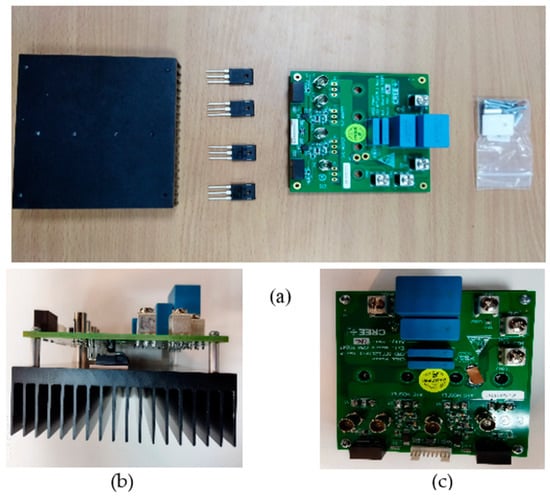
Figure 12.
(a): Package content of the SiC MOSFET evaluation kit, (b): side view of the mounted board, (c): top view of the mounted board.
3.2. Step 2: Choice of Control and Communication Boards
The choice of the control card can be performed taking into account several factors. Among them, one can quote: the price, the footprint, the processing performances and the supported communication protocols. In our case, the chosen control card is the F28335 Delfino Control Card from Texas Instruments (TI). This MCU belongs to the TI C2000 family, which is mainly dedicated to power system control applications [18].
As for the communication boards, one must note that in a WPT charger, not only is the power is transferred wirelessly, but also the communicated data between the ground side and vehicle side. Thus, the SAEJ2954 standard recommends the use of WiFi protocol to perform this communication. In this regard, the Raspberry Pi4 Model B is chosen. Note that unlike the previous versions, the Pi4 Model B version integrates a WiFi module (2.4 GHz and 5.0 GHz IEEE 802.11). Moreover, the Pi4 Model B supports several wired data communications such as UART (Universal Asynchronous Receiver/Transmitter), SPI (Serial Peripheral Interface) and I2C (Inter-Integrated Circuit). Thus, hardware support packages compatible with MATLAB/Simulink 2020 are already available, making the programming task much easier. Other sophisticated boards could also be used to perform the wireless communication task. However, the price is a decisive factor in our case.
3.3. Step 3: Design of Ground- and Vehicle-Side Coils
3.3.1. Conductor Wire Choice for Making Coils
The coil’s design task starts by selecting appropriate wires. Thus, in order to reduce the skin and proximity effect caused by the high operating frequency, WPT designers generally opt for a particular conductor wire known as a Litz wire [19]. This is formed by multi-strand twisted wires. These cables are classified according to the gauge, number of strands and operating frequency range. Note that the wire gauge increases as the operating frequency increases, whereas the strand diameter decreases. This means that the nature of the cable, for a given current intensity, differs according to the operating frequency. Indeed, for high-operating frequencies, the cable must contain several strands; however, the number of the strands decreases in the case of low frequencies. Since the WPT charger is operating at a frequency of 85 kHz, the AWG 38 (AWG for American Wire Gauge), characterized by a frequency range of 50 kHz to 100 kHz, is the recommended type for WPT chargers.
3.3.2. Coil Geometry Choice
Now to the geometry of the coils. It is worth noting that the circular and rectangular planar coils are the most commonly adopted geometries for making WPT chargers. Thus, in order to analyze the characteristics of each of these two coils, a comparative study was carried out in [20]. The study shows that, for a given air gap and the same coil’s size, the circular coils ensure high mutual inductance compared with the square ones. However, the square coils are more tolerable to misalignments. This makes circular coils best suited for stationary charging, while rectangular coils are recommended for dynamic charging [6,21]. With this in mind, the circular geometry is adopted in the current design.
3.3.3. Coil Inductance Calculation
Generally, the calculation of the coil inductance begins with setting the desired quality factor of the circuit on the vehicle side [22]. Note that a higher quality factor is generally desired to improve the circuit performance. Yet, in practice, higher quality factors require high inductance values. This, in turn, leads to a coil with large dimensions, which ultimately complicates its integration into the vehicle. That is, the quality factor will be set to 12.
Using (15), the required inductance can be calculated as follows:
Inserting the suitable values gives .
As for the primary coil, since a typical range of the coupling in a WPT charger varies between 0.1 and 0.4, an initial value of the inductance of the primary coil will be chosen as 360 µH. This gives an initial coupling .
The main reason behind choosing a higher inductance value for the ground side is due to the fact that the emitting coil needs to be larger than the receiving one in order to ensure a high mutual coupling even in the presence of alignment offsets.
3.3.4. Choice of Parameters, Simulation and Realization of Coils
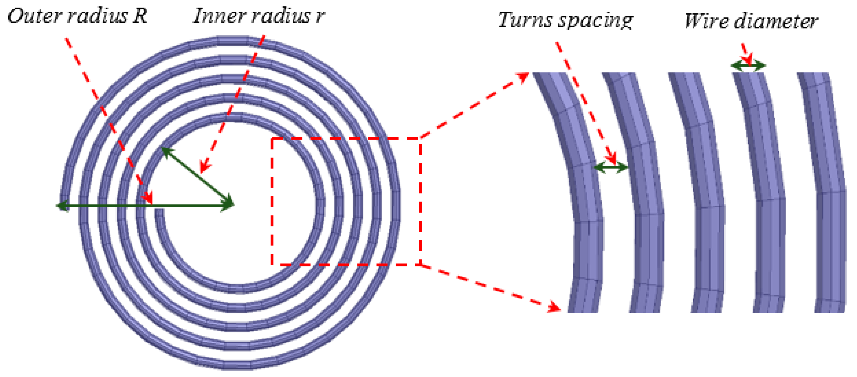
From the design viewpoint, the inner radius, the outer radius, the spacing between the turns and the number of turns of a circular planar coil are important parameters that must be chosen with care to achieve the desired performance (see Figure 13).
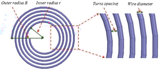
Figure 13.
Illustrative shape of a circular planar coil.
As indicated in [23], increasing the turns’ spacing makes it possible to achieve the desired inductance value with fewer turns. This makes it possible to reduce the length of the conductor wire, which ultimately reduces the weight and cost of the coil. However, the mutual coupling decreases as the spacing between the turns increases. For this reason, to ensure better coupling between the coils, we will try to bring the turns closer to each other in order to eliminate the spacing. In addition, since the diameter of the wire is already fixed, the number of turns and the inner and outer radii remain the only parameters to be adjusted to achieve the desired coil performance. That is, three coils with different geometries are proposed in our case. These are described as follows:
- Coil geometry 1 (hereinafter Coil1): this is the geometry of the ground-side coil. Its outer diameter is set to 48 cm. This choice is justified by the fact that the height of the created magnetic flux is approximately 1/4 of the outer diameter of the coil [23]. With this choice, for a nominal air gap of 12 cm, the coupling between the coils is ensured.
- Coil geometry 2 (hereinafter Coil2): this is the first geometry adopted for the coil on the vehicle side. Its outer diameter is set to 30 cm. The main reason for choosing a smaller diameter is to allow the vehicle-side coil to remain in the area covered by the ground-side coil even in the presence of misalignments.
- Coil geometry 3 (hereinafter Coil3): this is the second geometry adopted for the coil on the vehicle side. Its outer diameter is set to be the same as that of the ground-side coil (48 cm). This choice is justified assuming that the two coils must have the same external diameter so that all of the magnetic field created by the coil on the ground side will be captured by the one on the vehicle side.
Once the geometries are defined, the next step consists of calculating the number of turns necessary to achieve the desired inductances. To that end, the Wheeler formula, shown in (25), is used. This formula gives the desired inductance in µH when all of the dimensions are in cm.
where N, Dout and Din are, respectively, the number of turns, the outer diameter and the inner diameter of the coil.
The relations between Dout, Din and the diameter of the wire dw is given in the following:
The required length of the wire, in meters, can be calculated as follows:
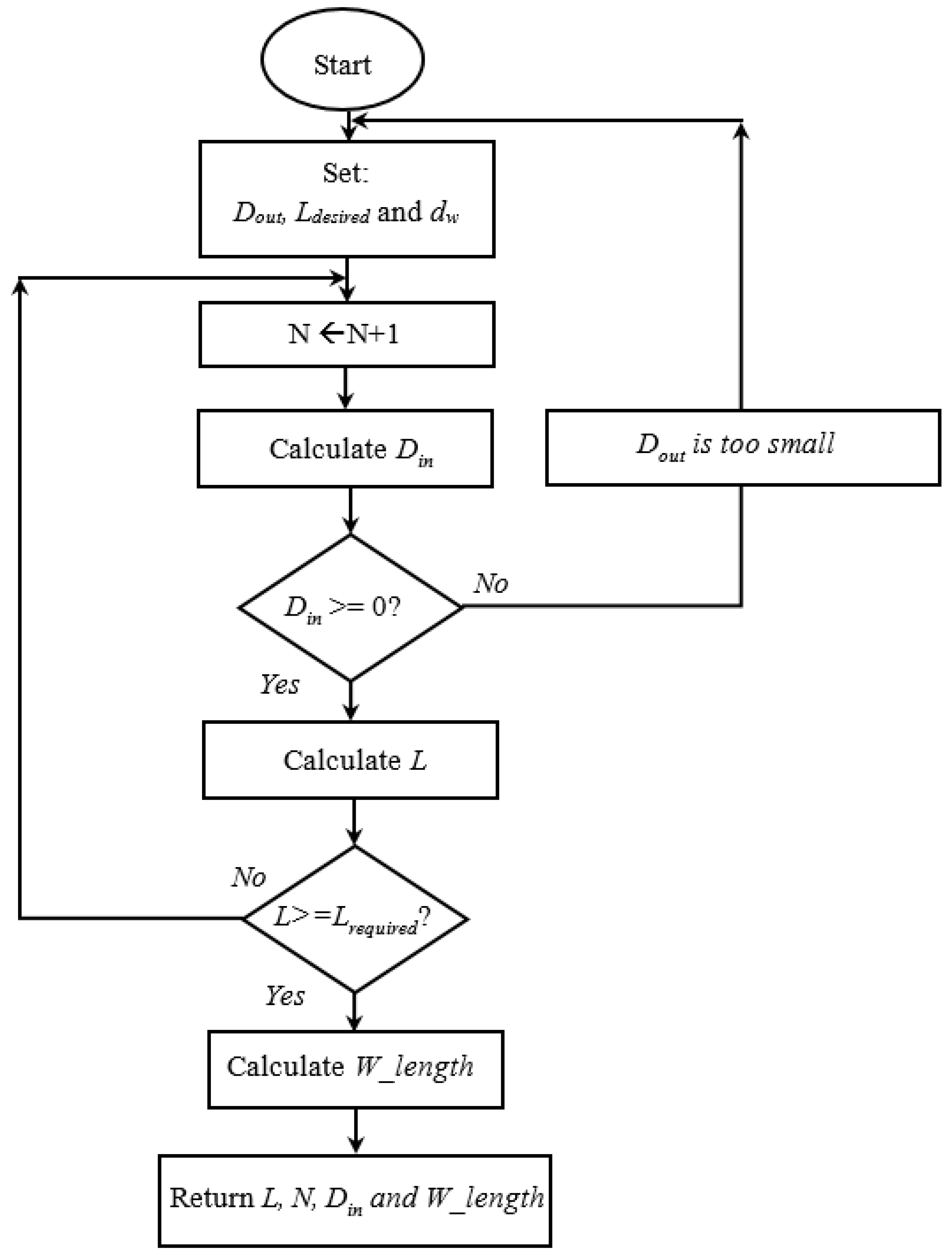
The calculation of the number of turns and the inner diameter for a required inductance is an iterative process in which we increment the number of turns and we calculate the corresponding Din and L. The process stops when the desired L is reached or if the calculated Din is negative. In the latter case, the initially chosen Dout is very small and needs to be increased. This is illustrated in the following flowchart (Figure 14).

Figure 14.
Flowchart of the iterative algorithm used to identify coil parameters.
For each of the geometries defined previously, the algorithm returns the following parameters shown in Table 3.
Table 3.
Summary of the calculated parameters for each geometry.
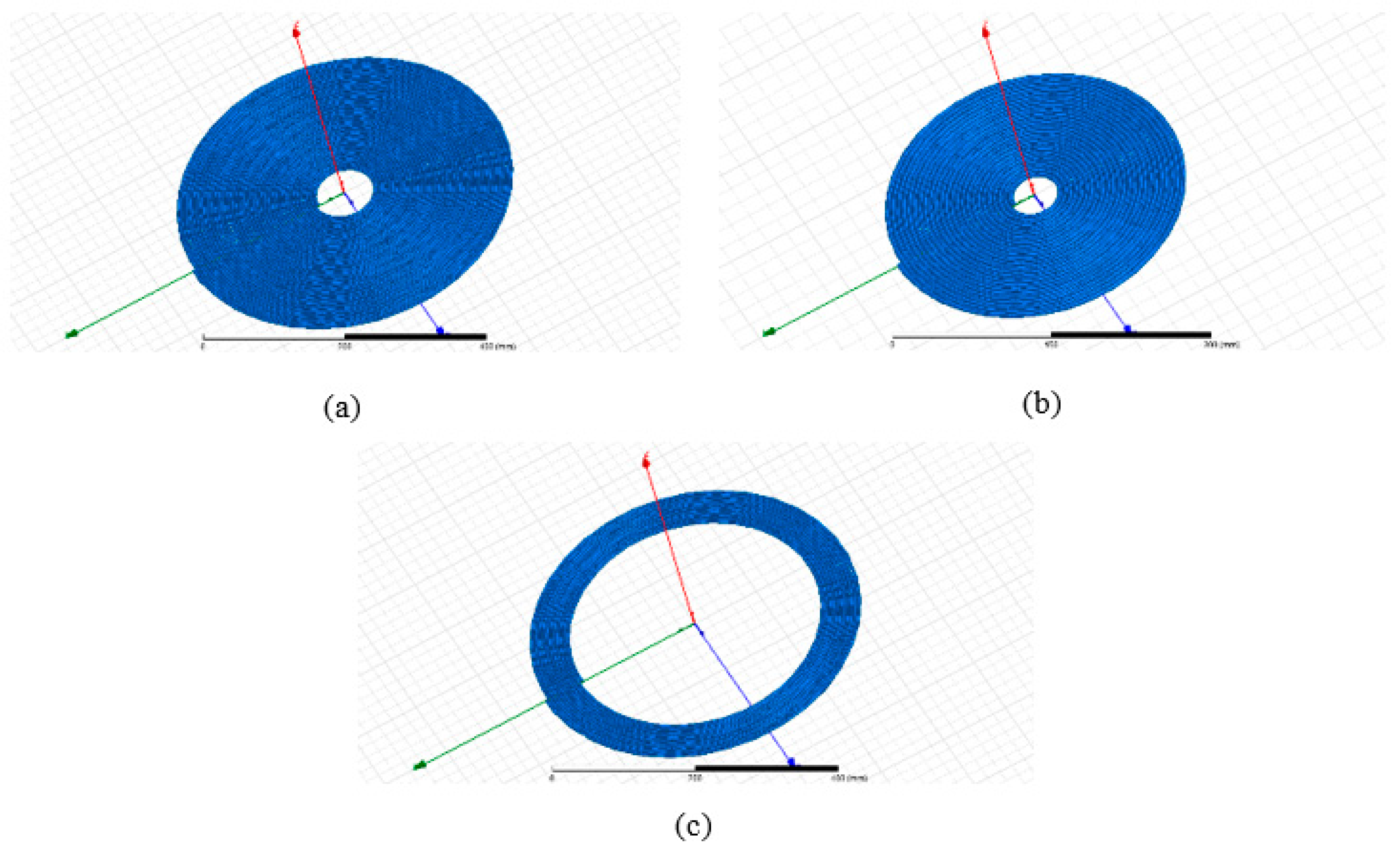
Before starting the realization task, one first needs to verify whether the calculated parameters will lead to the desired inductances, and also if the proposed coils will ensure the required coupling coefficient when the air gap varies in the interval range 100–150 mm. To that end, the Ansys/Maxwell software is used. That is, three coils, with the parameters listed in Table 3, were created as shown in the following figure (Figure 15).

Figure 15.
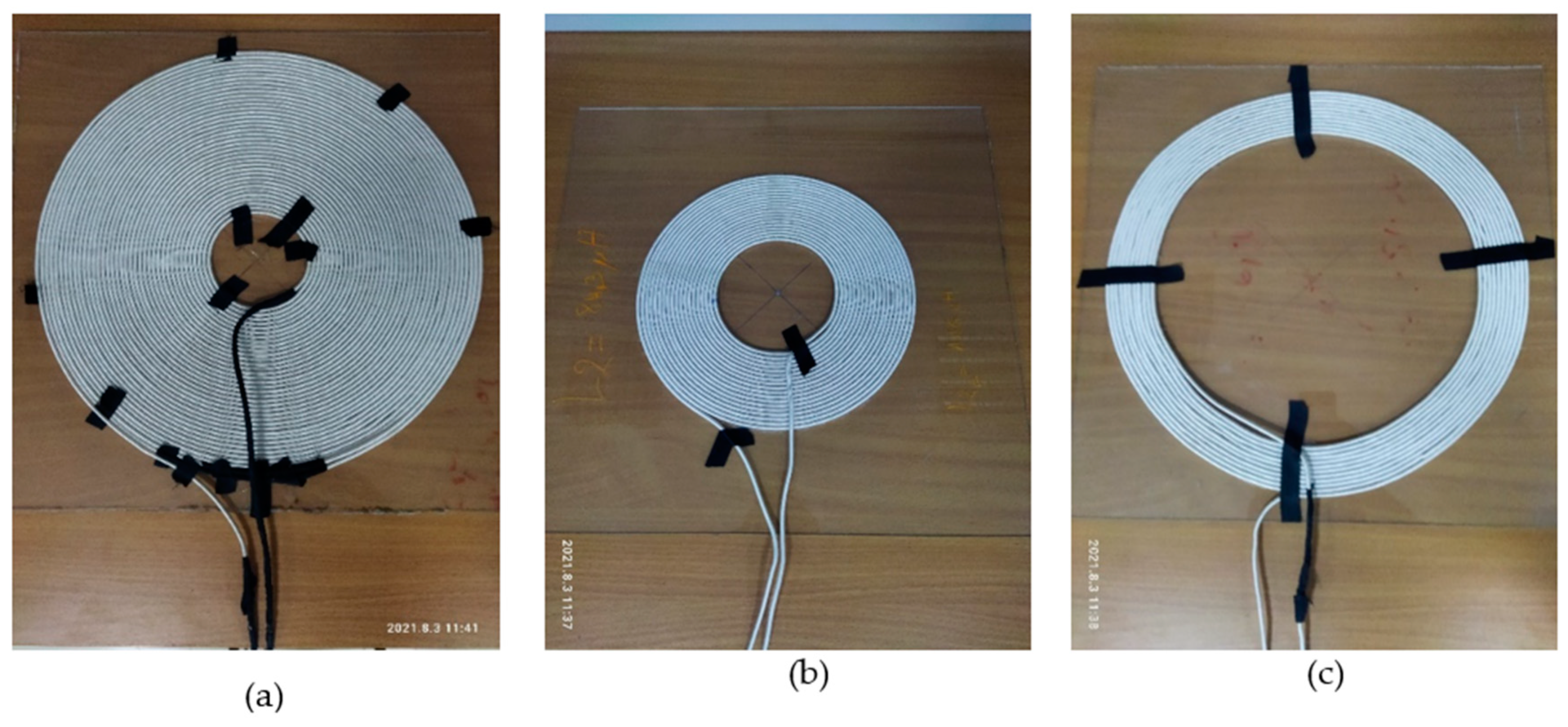
Images of the created coils using Ansys/Maxwell Software: (a): Coil1, (b): Coil2 and (c): Coil3.
The calculated inductances, using Ansys/Maxwell software, for each of the coil geometries 1, 2 and 3 are, respectively, 358.12 µH, 84.2 µH and 89.6 µH. We notice a slight difference between these values and those calculated using the Wheeler’s formula. This was expected, as the software performs the required calculations and simulations using finite elements analysis (FEA) methods which, in turn, depend on the used meshes, solver, etc.
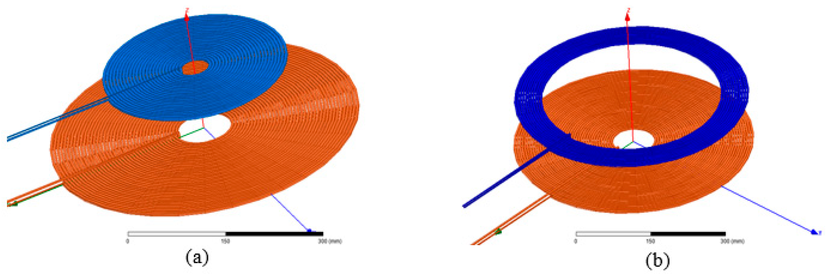
Once the inductances of the created coils have been verified, the next step consists of evaluating the coupling coefficient between the following pairs of coils: Coil1–Coil2 and Coil1–Coil3 (see Figure 16). To perform this test, using the Ansys/Maxwell software, one first needs to calculate the excitation currents of the ground-side coil (Coil1) and the vehicle-side coils (Coil2 and Coil3). These currents intensities are calculated as follows: and

Figure 16.
Image of the tested pairs of the coils: (a): Coil1–Coil2 and (b): Coil1–Coil3.
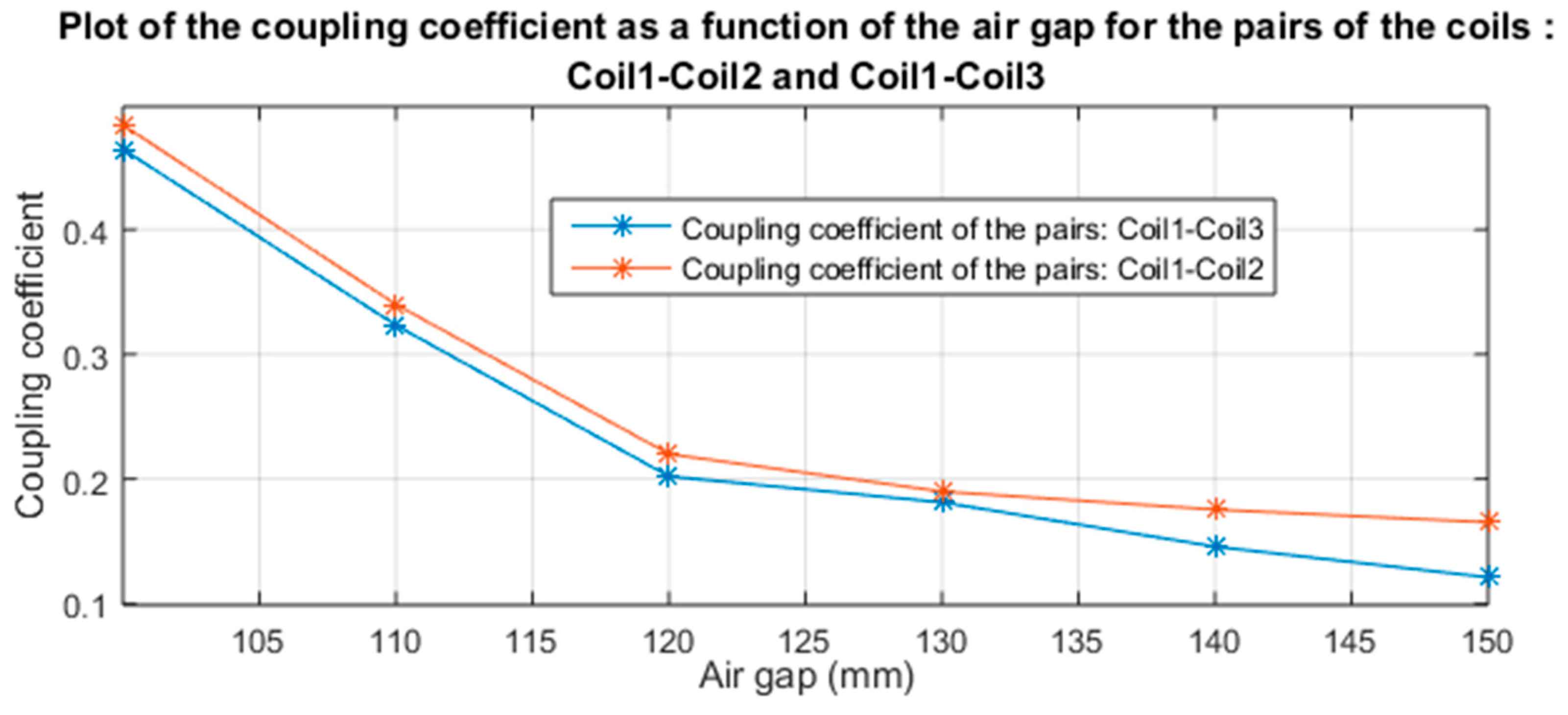
The evolution of the coupling coefficient for each of the pairs of coils is plotted in Figure 17. In this test, the air gap between the coils varies from 100 mm to 150 mm using a step of 10 mm. Note that this air-gap range corresponds to the Class Z1 of the SAEJ2954 standard. It can be seen from this figure that the two pairs of coils provide a coupling coefficient in the interval range 0.1–0.5. We can also notice that the coupling coefficient of the pair of coils Coil1–Coil2 is slightly higher than that of Coil1–Coil3.
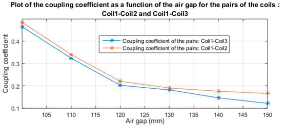
Figure 17.
Evolution of the coupling coefficient for the pairs of coils, Coil1–Coil2 and Coil1–Coil3, as a function of the air gap.
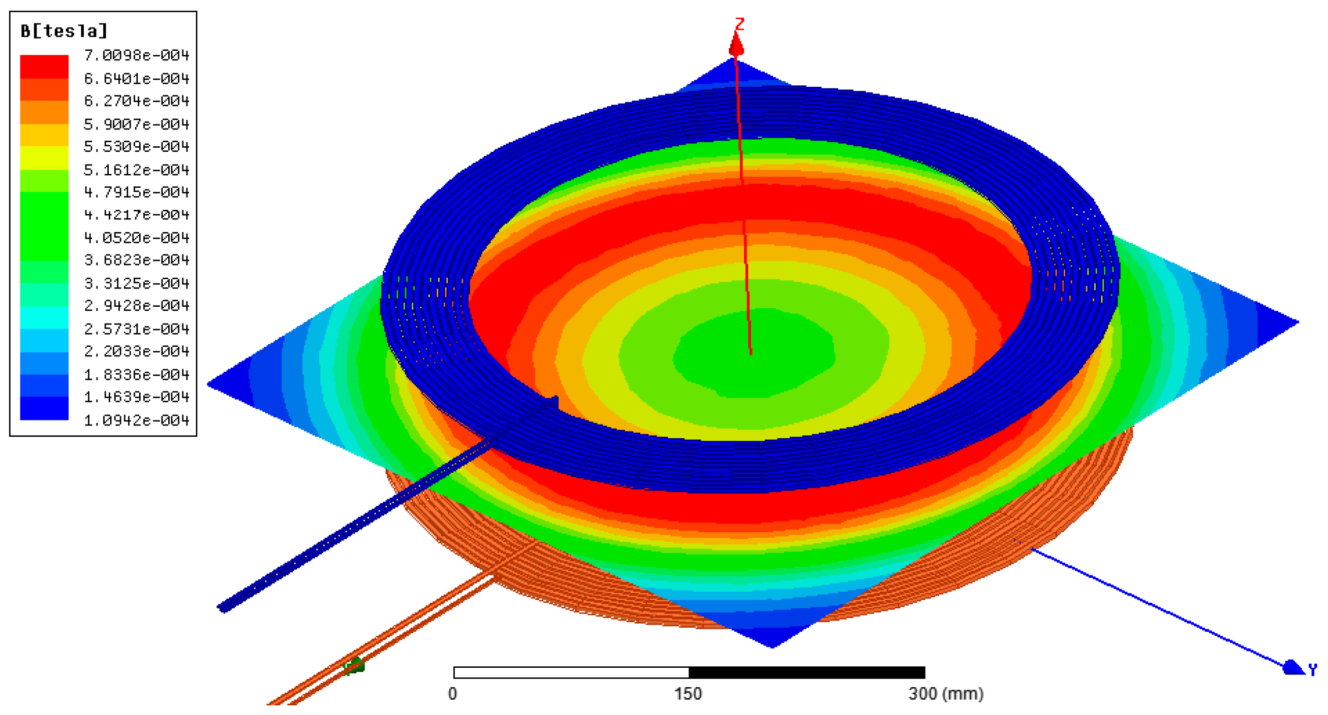
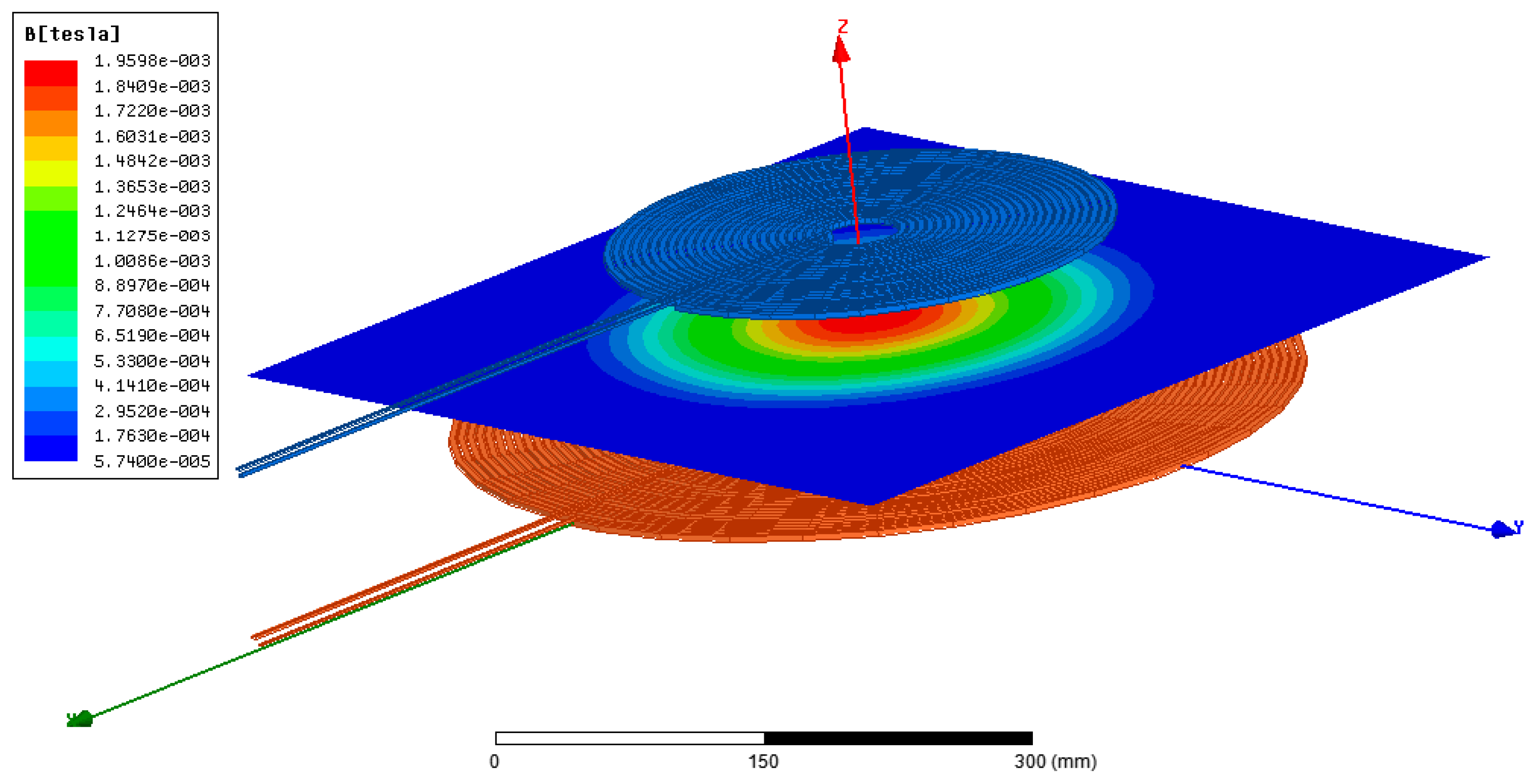
The magnetic field distribution of the two pairs of coils is plotted in Figure 18 and Figure 19. Two important remarks can be drawn from these figures. The first one is related to the intensity of the created magnetic field. Indeed, one can clearly see that the maximum magnitude of the magnetic field created by the Coil1–Coil2 pair is 1.9598 × 10⁻³, while that created by the other pair of coils is just 7.0098 × 10⁻⁴.
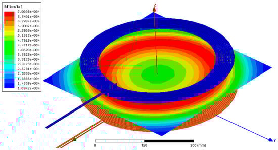
Figure 18.
Magnetic field distribution of the pair of coils Coil1–Coil3.
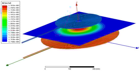
Figure 19.
Magnetic field distribution of the pair of coils Coil1–Coil2.
The second remark is related to the magnetic field distribution. Indeed, it can be seen that the peak amplitude occurs in the center of the pair Coil1–Coil2 and decreases as we approach the boundaries, while that of the Coil1–Coil3 pair occurs at the boundaries of the coils. This, a priori, leads us to say that the pair Coil1–Coil2 will ensure better performance even in the presence of alignment offsets.
The three coils have been fabricated in practice (see Figure 20). The main objective is to experimentally test different coil combinations in order to find the coil pair that gives the best performance in terms of power transfer efficiency and misalignment tolerance.
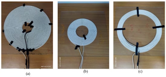
Figure 20.
Fabricated coils: (a): Coil1, (b): Coil2 and (c): Coil3.
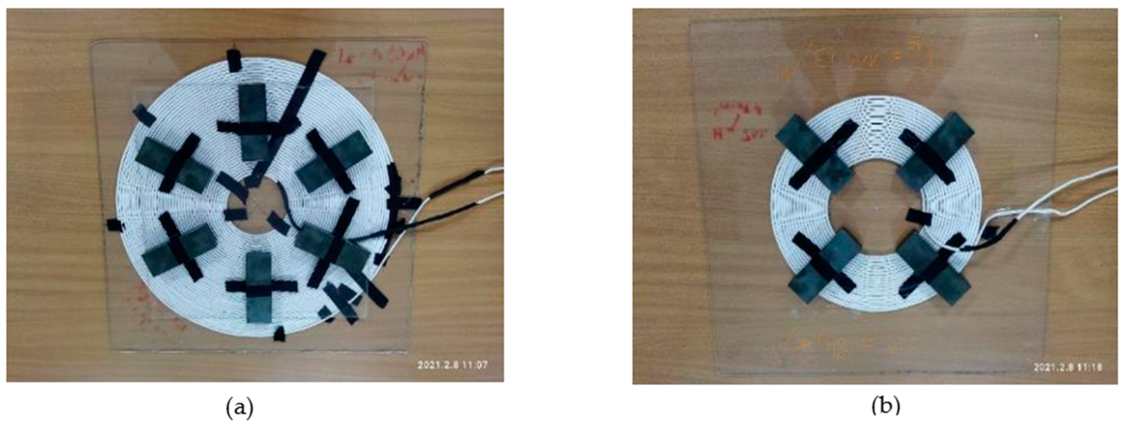
Note that ferrite cores have been added to the coils in order to guide the magnetic flux from the transmitting coil to the receiving one. In this regard, it should be noted that the arrangement of the ferrite cores on the coil is of great importance, as a worse arrangement could decrease the power transfer efficiency. Thus, as expected, the addition of the ferrite to the coils (see Figure 21) increases their inductances. Indeed, the measured inductance for Coil1, with six ferrite cores mounted on its bottom side, is 416 µH, while that measured for Coil2 and Coil3, with four ferrite cores mounted on their top sides, is 116 µH.

Figure 21.
Fabricated coils with ferrite cores: (a): Coil1 and (b): Coil2.
3.4. Step 4: Design of Ground- and Vehicle-Side Compensation Boards
The role of the compensation blocks is to cancel out the reactive impedance of the WPT circuit, which reduces the reactive energy and increases the overall efficiency. The series–series compensation topology, adopted in our case, is commonly used in the literature due to the fact that the calculated capacitance values are independent of the load and mutual inductance. The required capacitance is calculated as follows:
Thus, the maximum voltages occurring across these capacitors are calculated as follows:
The design of the compensation capacitor board must be performed carefully. On the one hand, it must be designed to ensure the condition of resonance with the coil, and on the other hand, it must withstand the involved high voltages. A general design approach is presented as follows.
Assuming similar capacitors are used, the total capacitance of a compensation bloc containing Np parallel-connected branches where each branch contains an NS series-connected capacitor is given by the following expression:
where C is the capacitance of one capacitor and CT is the desired compensation capacitance.
First, to comply with the high-voltage constraint, the required number of series capacitors can be calculated as follows:
where VMAX is the maximum operating voltage of one capacitor, and Vc,MAX is the maximum voltage occurring across the compensation network.
Assuming, for example, that a 100 nF, a 500 VAC polypropylene capacitor is chosen for making the vehicle-side compensation bloc. Then, NS can be calculated as follows:
To ensure the safe operation of the capacitors, NS will be chosen to be 3. With this choice, the required parallel branches will be calculated using (28), as follows:
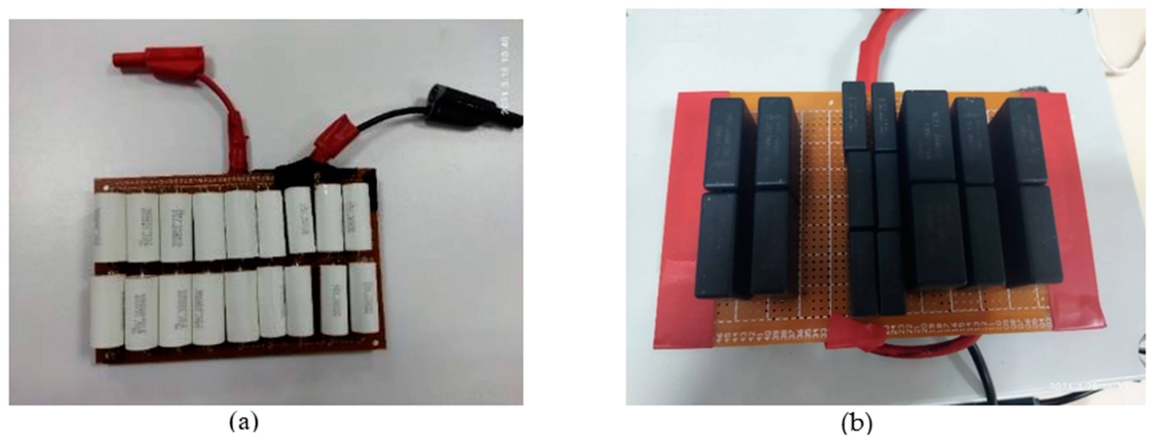
The realized grid-side and vehicle-side compensation boards are illustrated in Figure 22. In our case, depending on the available components, capacitors with different values are used. Thus, the measured capacitance values of the compensation boards in the ground and vehicle sides are, respectively, C1 = 8.9 nF and C2 = 31.5 nF. These values lead to two resonance frequencies: f1 = 82,713 Hz and f2 = 83,259 Hz. Following this, the resonance frequency is chosen as the mean value of f1 and f2. That is, f = (f1 + f2)/2 = 82,986 Hz, which is in the interval range recommended by the SAEJ2954 standard (81–91 kHz).
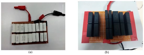
Figure 22.
Images of the realized compensation boards (a): in the vehicle side and (b): in the ground side.
4. Experimental Results
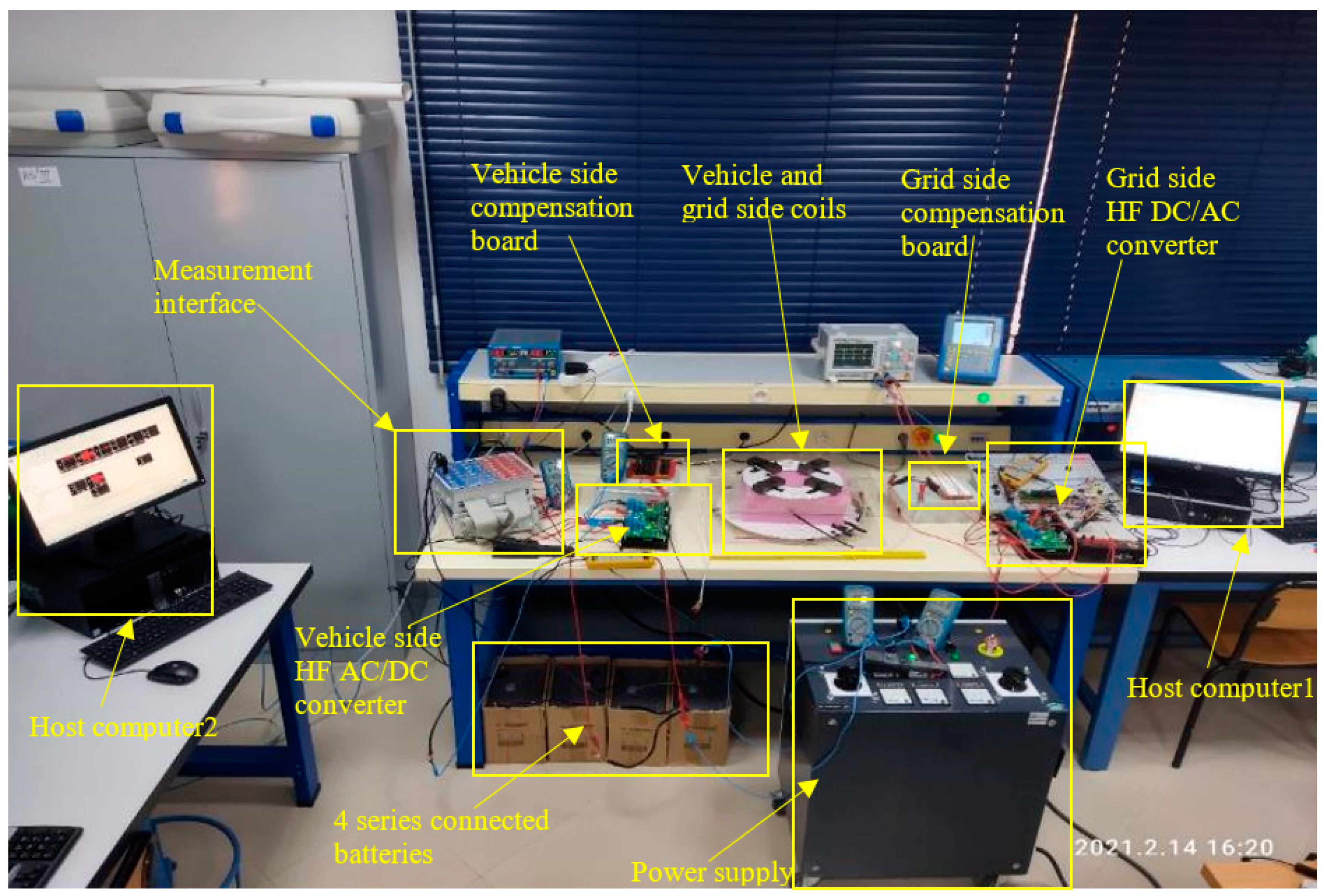
The overall experimental setup of the realized WPT charger is shown in Figure 23. In order to validate the design procedure, several tests were realized on the basis of this setup. The obtained results are presented and discussed in the sequel.
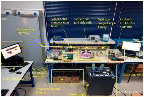
Figure 23.
Overall setup of the realized DC–DC WPT charger.
4.1. Test of the Realized Coils
The main objective of this test is to find the coil’s pair that ensures optimal efficiency. To that end, the realized coils are subjected to several test scenarios. It should be noted that the variation of the air gap and misalignments between the coils leads to different values of the mutual inductances, which finally gives rise to different power transfer. The latter is specified for each test scenario.
- Scenario 1: The coils are perfectly aligned and spaced from each other with a distance of ΔZ = 12 cm. In this case, a power of 300W is transferred from the ground side to the vehicle side; thus, the obtained power transfer efficiency is 95% for the pair of coils Coil1–Coil2, while that of Coil1–Coil3 is 89.5%.
- Scenario 2: The coils are laterally misaligned in both directions (ΔX = 7 cm and ΔY = 10 cm) while the air gap between the coils is maintained at ΔZ = 12 cm. In this case, a power of 500 W is transferred from the ground side to the vehicle side; thus, the obtained power transfer efficiency is 89% for the pair of coils Coil1–Coil2, while that of Coil1–Coil3 is 78%.
- Case 3: The air gap is maintained at its maximum (ΔZ = 15 cm) and the coils are misaligned in both directions (ΔX = 7 cm and ΔY = 10 cm). In this case, a power of 900 W is transferred from the ground side to the vehicle side; thus, the obtained power transfer efficiency is 83.5% for the pair of coils Coil1–Coil2, while that of Coil1–Coil3 is 72%.
Based on the obtained results, one can clearly see in Figure 24 that the pair Coil1–Coil2 presents good power transfer efficiency. Indeed, the lowest measured efficiency is 83.5%. This value was obtained for the worst-case positioning of the coils corresponding to scenario 3, in which the coils are misaligned in both directions and largely spaced between each other. It should be noted that this efficiency remains above the minimum limit of the SAEJ2954.
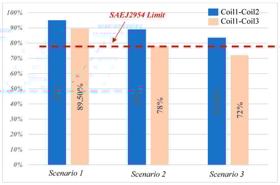
Figure 24.
WPT efficiencies for different scenarios of the coil pairs.
The pair Coil1–Coil3 presents lower performances, as was expected, since the simulation stage was performed using Ansys/Maxwell software. With this in mind, the pair Coil1–Coil2 is retained for the rest of the tests.
4.2. Effect of Variation of DC Side Voltage on Power Transfer
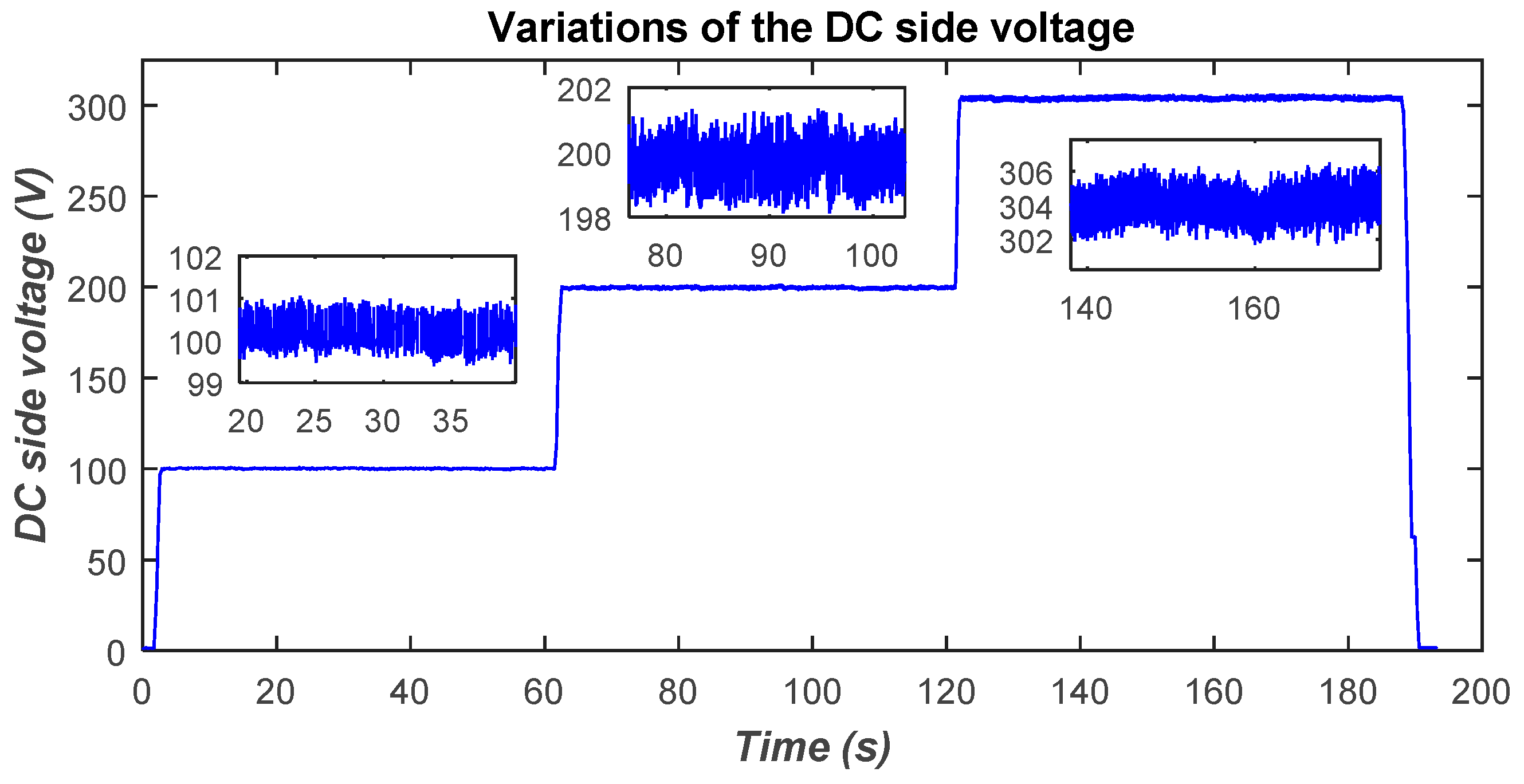
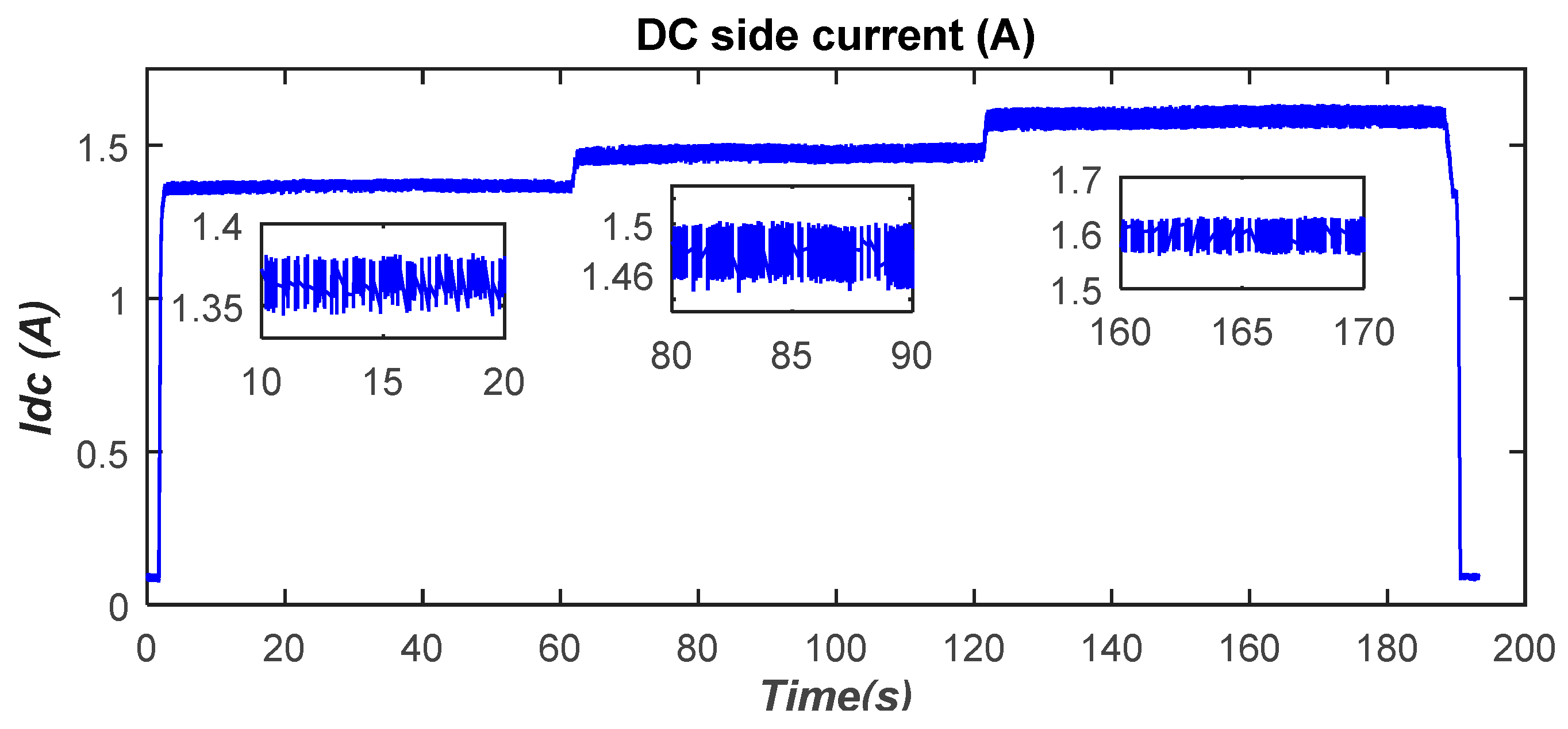
In this test, the two coils are perfectly aligned and spaced at a distance of 120 mm. It should be noted that this distance has been identified as that which gives rise to a mutual coupling of approximately 44 µH, which is necessary for transferring a power of 500 W. The main objective is to study the effect of the DC-side voltage on the amount of power transferred to the battery. To that end, the DC-side voltage was varied, using a variable DC power supply, from 100 V to 300 V with a step of 100 V. This is shown in Figure 25. The corresponding DC-side current variations are shown in Figure 26.

Figure 25.
DC-side voltage variations.

Figure 26.
DC-side current variations.
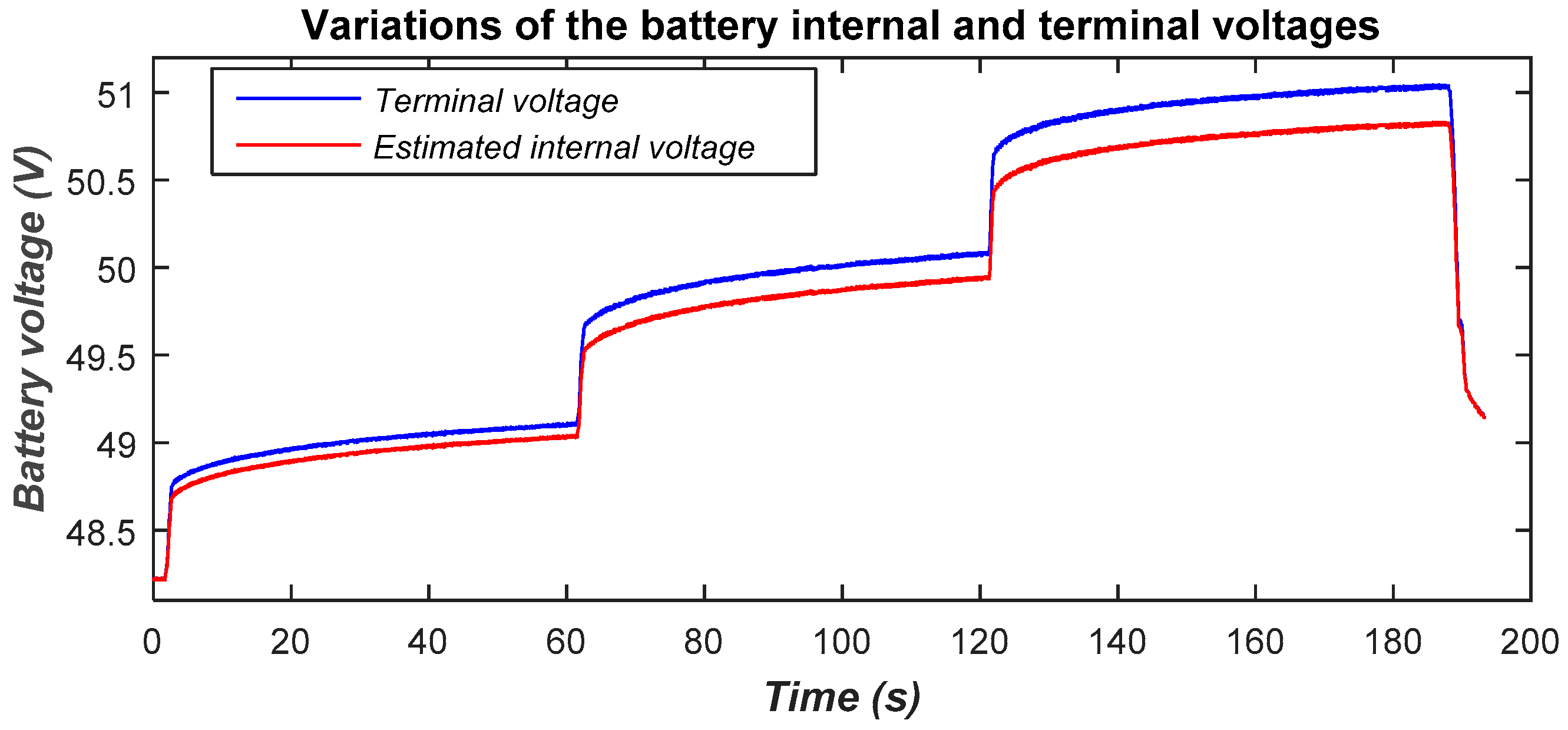
Figure 27 shows the battery terminal and estimated internal voltage variations. The internal battery voltage was estimated using the equivalent internal series resistance (ESR) of the battery. Indeed, according to the manufacturer, the ESR was estimated at 0.0063 Ω (4 × 0.0063 Ω for four series connected batteries). As is known, the ESR of a battery can vary depending on several factors such as the aging of the battery and the operating temperature. It is assumed that all of these factors do not affect the ESR value, since newer batteries are used and their internal temperature could also be assumed to be constant during experiments.
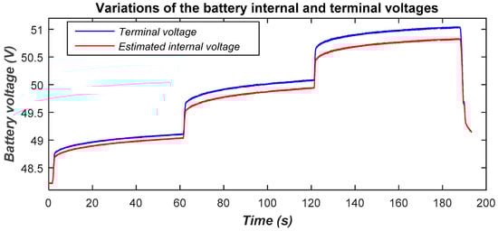
Figure 27.
Battery terminal and internal voltages.
The gap between the two voltages increases as the battery-charging current increases due to the voltage drop caused by the equivalent series resistance.
The battery-charging current is plotted in Figure 28. One can see that it depends on the DC-side voltage. Indeed, the battery-charging current changes as the DC-side voltage is stepped from one voltage level to another. That is, the maximum achievable charging current, under the perfect alignment of the coils and for a fixed air gap of 12 cm, is approximately 8.5 A.
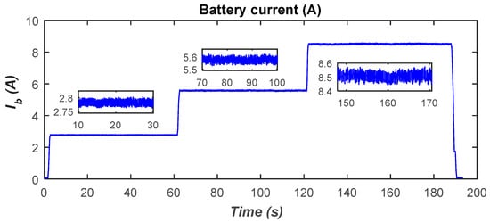
Figure 28.
Battery-charging current variations.
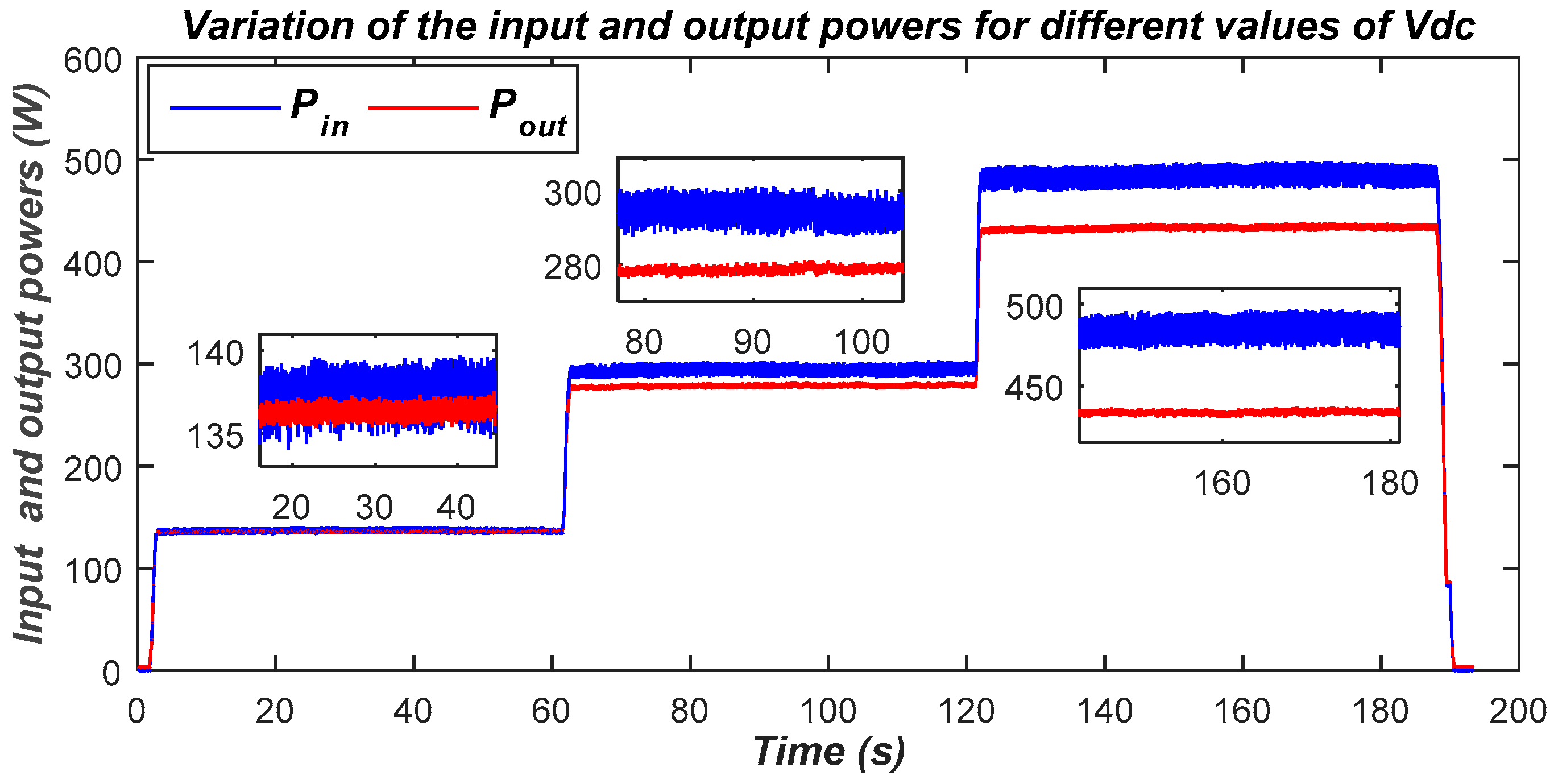
The power transferred from the DC side (input power) and the battery-charging power (output power) are plotted in Figure 29. A trivial remark that could be drawn from this figure is that the amount of power that can be transferred depends on the voltages on the DC side and the battery side. As the latter is kept constant, the transferred power can only be adjusted by acting on the voltage on the DC side. Thus, a maximum power of approximately 500 W is achieved when the DC-side voltage is set at its maximum of 300 V.
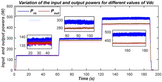
Figure 29.
DC-side and battery-side power variations.
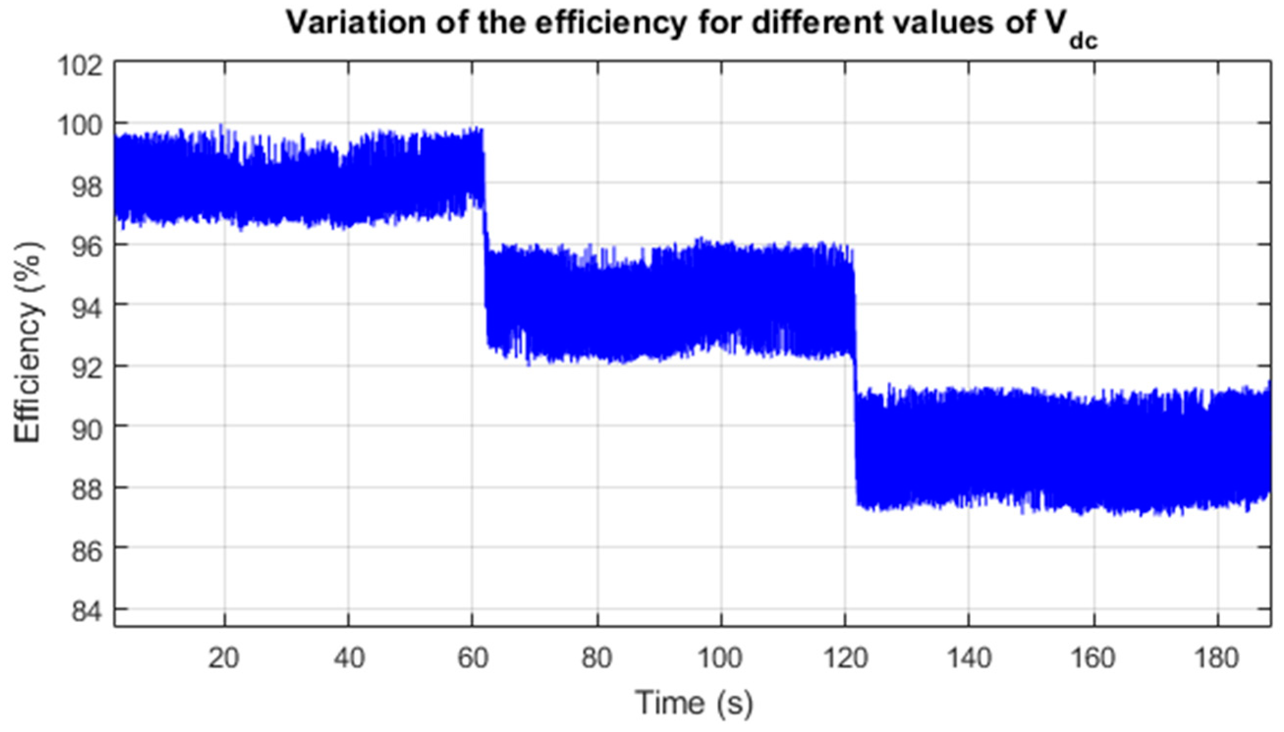
The efficiency variations are plotted in Figure 30. It is noticed that the efficiency decreases as the transferred power increases. Indeed, the efficiency passes from approximately 97% (for a power of 140 W) to 90% (for a power of 500 W).

Figure 30.
Power transfer efficiency variations.
4.3. Effect Misalignments on Power Transfer
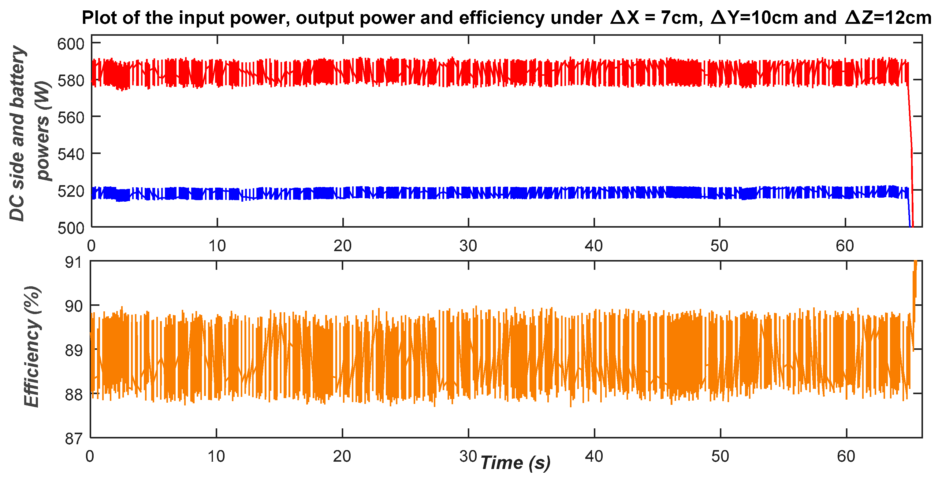
The main objective of the present test is to check the effect of the misalignments on the amount of transferred power. To that end, two test scenarios are performed. In the first one, the coils are laterally misaligned (Δx = 7 cm and Δy = 10 cm), while the air gap is kept at 12 cm. That is, the DC-side and the battery-side powers reach, respectively, approximately 590 W and 520 W, while the corresponding efficiency is about 89% (see Figure 31).
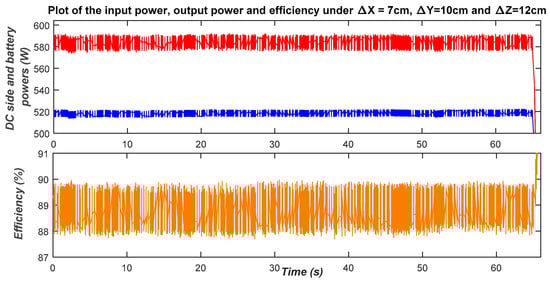
Figure 31.
Variations of the DC-side power, battery power and efficiency in the presence of lateral misalignments (Vdc = 200 V, Δx = 7 cm, Δy = 10 cm and Δz = 12 cm).
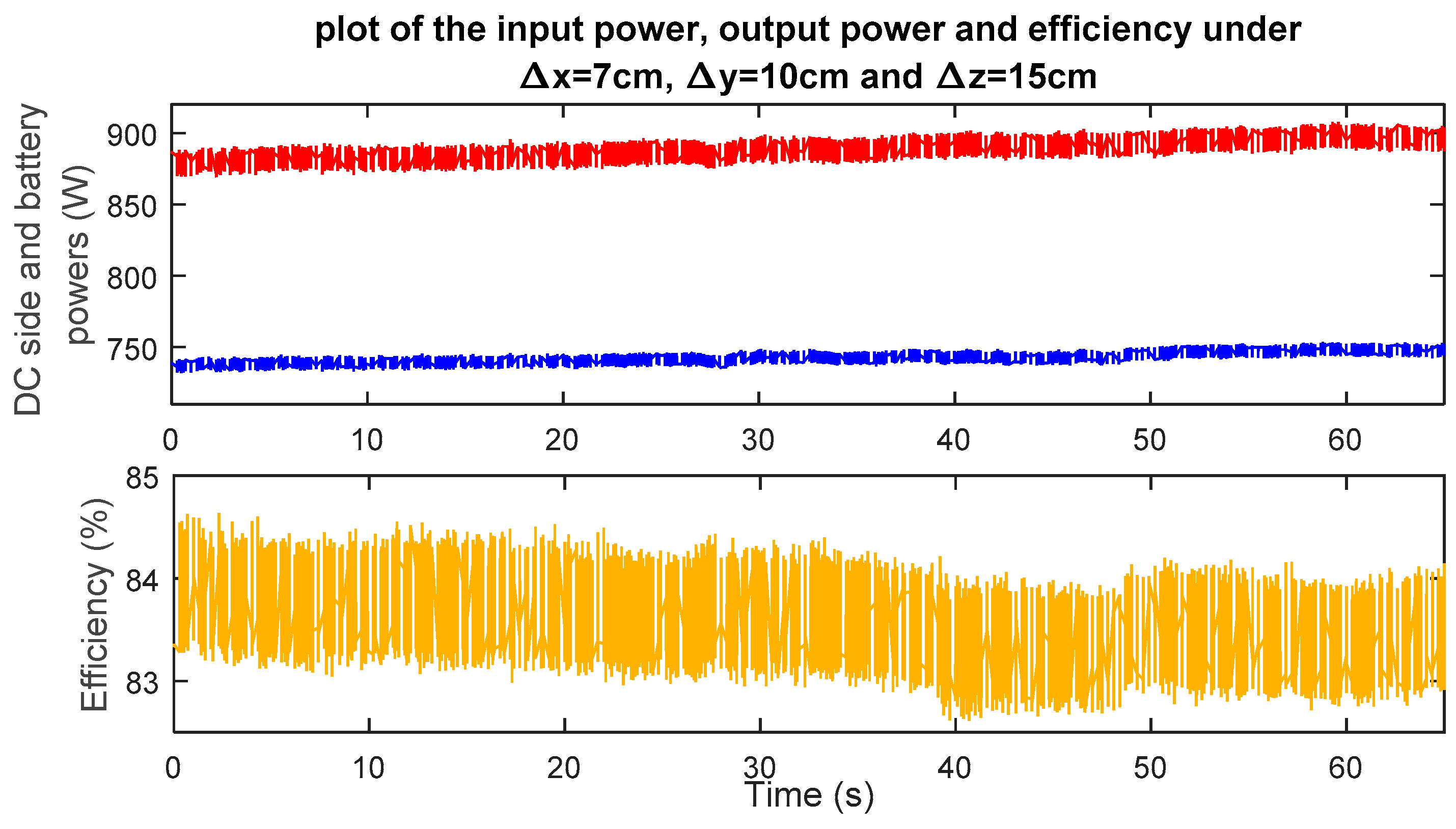
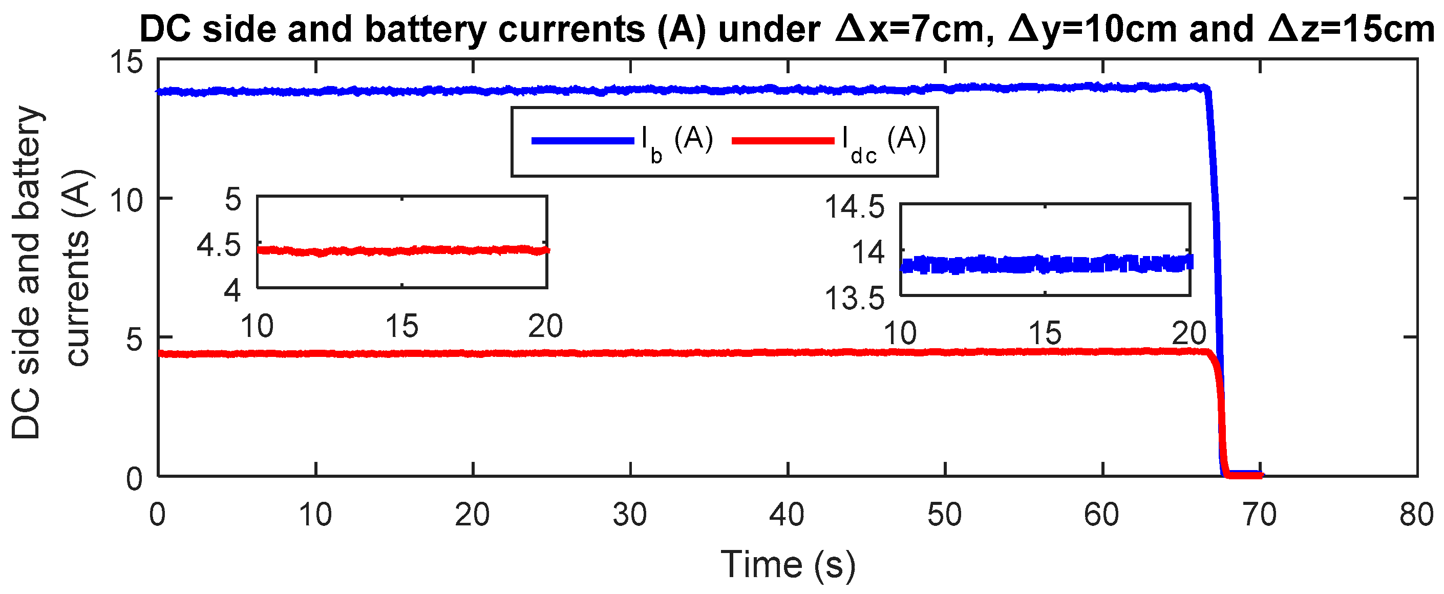
In the second scenario, both lateral and vertical misalignments are considered (Δx = 7 cm, Δy = 10 cm and Δz = 15 cm). This could be considered as the worst positioning case. In this test, the DC side and the battery powers reach, respectively, approximately 900 W and 750 W while the corresponding efficiency is about 83% (see Figure 32). Thus, the corresponding DC-side and battery-charging currents are plotted in Figure 33, in which we notice a maximum charging current of approximately 14 A.

Figure 32.
Variations of the DC-side power, battery power and efficiency in the presence of lateral and vertical misalignments (Vdc = 200 V, Δx = 7 cm, Δy = 10 cm and Δz = 15 cm).
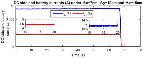
Figure 33.
Variations of the DC-side and battery currents in the presence of lateral and vertical misalignments (Vdc = 200 V, Δx = 7 cm, Δy = 10 cm and Δz = 15 cm).
These tests reveal that the power transfer increases in the presence of misalignments. This is due to the fact that the mutual coupling decreases as far as the misalignments increase. Therefore, according to (24), lower mutual coupling will lead to an increase in power transfer.
In all of these tests, the DC-side voltage is maintained at a value of 200 V. The main reason for choosing 200 V rather than 300 V is due to the fact that the latter value, in the presence of misalignments, could lead to high currents in the ground- and vehicle-side coils, which ultimately generate high voltages across the compensation capacitors. Thus, to ensure the safe operation of these capacitors, the DC-side voltage is maintained at 200 V.
5. Conclusions
This paper deals with WPT chargers for EVs. Firstly, the effect of the varying parameters on the operation of the WPT charger was investigated. It was found that the operating frequency, DC-side and battery-side voltage levels, compensation network and mutual inductance are key parameters that affect the power transfer capability and efficiency of the charger. Secondly, the design and realization of a 500 W WPT laboratory prototype was addressed. Due to the necessity of high-frequency switching, the SiC MOSFET transistors were chosen for making the power converters as they significantly reduce the power losses. As for the controllers, the C2000 F28335 MCU and Raspberry Pi4 were chosen due to their dedicated power control and communication features. Concerning the ground-side and vehicle-side coils, firstly, the adequate conductor wire and appropriate geometries were selected. Then, the proposed coils were simulated using Ansys/Maxwell software. The obtained simulation results showed that one pair of the coils presented better performance than the other. The proposed coils were realized, and then, based on their inductances, adequate series compensation boards were designed and realized. The overall WPT charger setup was tested, in open-loop mode, using a 48 V battery pack. The obtained results showed that the charger ensures good efficiency (around 90%) in an optimal working scenario, while the efficiency of the worst-case scenario was estimated at around 83%, which is above the SAEJ2954 limit.
Regarding the perspectives of the present work, the control task of the WPT charger will be addressed. Indeed, we plan to develop different control approaches for the WPT charger where the controllers could be implemented either on the ground side or on the vehicle side. A dual-control approach is also envisaged. The main objective is to compare the advantages of each approach in order to identify the most appropriate control strategy for the WPT charger.
Author Contributions
Formal analysis, H.E.F. and A.R.; methodology, H.E.F., T.B. and Z.E.I.; resources, A.M.H.; software, A.L.; supervision, H.E.F.; validation, A.L.; visualization, Z.E.I.; writing—original draft, I.B. and A.L. All authors have read and agreed to the published version of the manuscript.
Funding
This research was funded by IRESEN (Moroccan Research Institute for Solar Energy and New Energies) under grant INNO-PROJECT 2018/CBSCVEV2X.
Data Availability Statement
Not applicable.
Acknowledgments
The authors gratefully acknowledge the support of the IRESEN (Moroccan Research Institute for Solar Energy and New Energies) under grant INNO-PROJECT 2018/CBSCVEV2X.
Conflicts of Interest
The authors declare no conflict of interest.
References
- Unterluggauer, T.; Rich, J.; Andersen, P.B.; Hashemi, S. Electric vehicle charging infrastructure planning for integrated transportation and power distribution networks: A review. eTransportation 2022, 12, 100163. [Google Scholar] [CrossRef]
- Lassioui, A.; El Fadil, H.; Belhaj, F.Z.; Rachid, A. Battery Charger for Electric Vehicles Based ICPT and CPT—A State of the Art. In Proceedings of the 2018 Renewable Energies, Power Systems Green Inclusive Economy (REPS-GIE), Casablanca, Morocco, 23–24 April 2018; pp. 1–6. [Google Scholar] [CrossRef]
- Shareef, H.; Islam, M.; Mohamed, A. A review of the stage-of-the-art charging technologies, placement methodologies, and impacts of electric vehicles. Renew. Sustain. Energy Rev. 2016, 64, 403–420. [Google Scholar] [CrossRef]
- Gnann, T.; Funke, S.; Jakobsson, N.; Plötz, P.; Sprei, F.; Bennehag, A. Fast charging infrastructure for electric vehicles: Today’s situation and future needs. Transp. Res. Part Transp. Environ. 2018, 62, 314–329. [Google Scholar] [CrossRef]
- Biresselioglu, M.E.; Demirbag Kaplan, M.; Yilmaz, B.K. Electric mobility in Europe: A comprehensive review of motivators and barriers in decision making processes. Transp. Res. Part Policy Pract. 2018, 109, 1–13. [Google Scholar] [CrossRef]
- Bouanou, T.; El Fadil, H.; Lassioui, A.; Assaddiki, O.; Njili, S. Analysis of Coil Parameters and Comparison of Circular, Rectangular, and Hexagonal Coils Used in WPT System for Electric Vehicle Charging. World Electr. Veh. J. 2021, 12, 45. [Google Scholar] [CrossRef]
- Lukic, S.M.; Pantic, Z. Cutting the Cord: Static and Dynamic Inductive Wireless Charging of Electric Vehicles. Electrif. Mag. IEEE 2013, 1, 57–64. [Google Scholar] [CrossRef]
- Jayalath, S.; Khan, A. Design, Challenges, and Trends of Inductive Power Transfer Couplers for Electric Vehicles: A Review. IEEE J. Emerg. Sel. Top. Power Electron. 2021, 9, 6196–6218. [Google Scholar] [CrossRef]
- Hwang, Y.J.; Kim, J.M. A Double Helix Flux Pipe-Based Inductive Link for Wireless Charging of Electric Vehicles. World Electr. Veh. J. 2020, 11, 33. [Google Scholar] [CrossRef] [Green Version]
- Zimmer, S.; Helwig, M.; Lucas, P.; Winkler, A.; Modler, N. Investigation of Thermal Effects in Different Lightweight Constructions for Vehicular Wireless Power Transfer Modules. World Electr. Veh. J. 2020, 11, 67. [Google Scholar] [CrossRef]
- Berger, A.; Agostinelli, M.; Vesti, S.; Oliver, J.A.; Cobos, J.A.; Huemer, M. A Wireless Charging System Applying Phase-Shift and Amplitude Control to Maximize Efficiency and Extractable Power. IEEE Trans. Power Electron. 2015, 30, 6338–6348. [Google Scholar] [CrossRef]
- Mahesh, A.; Chokkalingam, B.; Mihet-Popa, L. Inductive Wireless Power Transfer Charging for Electric Vehicles—A Review. IEEE Access 2021, 9, 137667–137713. [Google Scholar] [CrossRef]
- Lassioui, A.; Fadil, H.E.; Rachid, A.; El-Idrissi, Z.; Bouanou, T.; Belhaj, F.Z.; Giri, F. Modelling and sliding mode control of a wireless power transfer system for BEV charger. Int. J. Model. Identif. Control 2020, 34, 171–186. [Google Scholar] [CrossRef]
- Lassioui, A.; El Fadil, H.; Rachid, A.; Bouanou, T.; Giri, F. Adaptive Output Feedback Nonlinear Control of a Wireless Power Transfer Charger for Battery Electric Vehicle. J. Control Autom. Electr. Syst. 2021, 32, 492–506. [Google Scholar] [CrossRef]
- Aditya, K.; Williamson, S.S. Design Guidelines to Avoid Bifurcation in a Series–Series Compensated Inductive Power Transfer System. IEEE Trans. Ind. Electron. 2019, 66, 3973–3982. [Google Scholar] [CrossRef]
- Wang, C.-S.; Covic, G.A.; Stielau, O.H. Power transfer capability and bifurcation phenomena of loosely coupled inductive power transfer systems. IEEE Trans. Ind. Electron. 2004, 51, 148–157. [Google Scholar] [CrossRef]
- Gallium Nitride (GaN) versus Silicon Carbide (SiC). Available online: https://www.richardsonrfpd.com/docs/rfpd/Microsemi-A-Comparison-of-Gallium-Nitride-Versus-Silicon-Carbide.pdf (accessed on 28 August 2020).
- TMDSCNCD28335 Daughter Card|TI.com. Available online: https://www.ti.com/tool/TMDSCNCD28335 (accessed on 20 September 2021).
- Kim, H.; Song, C.; Kim, D.-H.; Jung, D.H.; Kim, I.-M.; Kim, Y.-I.; Kim, J.; Ahn, S.; Kim, J. Coil Design and Measurements of Automotive Magnetic Resonant Wireless Charging System for High-Efficiency and Low Magnetic Field Leakage. IEEE Trans. Microw. Theory Tech. 2016, 64, 383–400. [Google Scholar] [CrossRef]
- Luo, Z.; Wei, X. Mutual Inductance Analysis of Planar Coils with Misalignment for Wireless Power Transfer Systems in Electric Vehicle. In Proceedings of the 2016 IEEE Vehicle Power and Propulsion Conference (VPPC), Hangzhou, China, 17–20 October 2016; pp. 1–6. [Google Scholar] [CrossRef]
- Bouanou, T.; Fadil, H.E.; Lassioui, A. Analysis and Design of Circular Coil Transformer in a Wireless Power Transfer System for Electric Vehicle Charging Application. In Proceedings of the 2020 International Conference on Electrical and Information Technologies (ICEIT), Rabat, Morocco, 7–7 March 2020; pp. 1–6. [Google Scholar] [CrossRef]
- Buja, G.; Bertoluzzo, M.; Mude, K.N. Design and Experimentation of WPT Charger for Electric City Car. IEEE Trans. Ind. Electron. 2015, 62, 7436–7447. [Google Scholar] [CrossRef]
- Aditya, K. Design and Implementation of an Inductive Power Transfer System for Wireless Charging of Future Electric Transportation. Ph.D. Thesis, University of Ontario Institute of Technology, Oshawa, ON, Canada, 2016. Available online: http://ir.library.dc-uoit.ca/handle/10155/712 (accessed on 14 September 2014).


Publisher’s Note: MDPI stays neutral with regard to jurisdictional claims in published maps and institutional affiliations. |
© 2022 by the authors. Licensee MDPI, Basel, Switzerland. This article is an open access article distributed under the terms and conditions of the Creative Commons Attribution (CC BY) license (https://creativecommons.org/licenses/by/4.0/).