
Implementation of Driving Cycles Based on Driving Style Characteristics of Autonomous Vehicles


Abstract
:1. Introduction
2. State of the Art
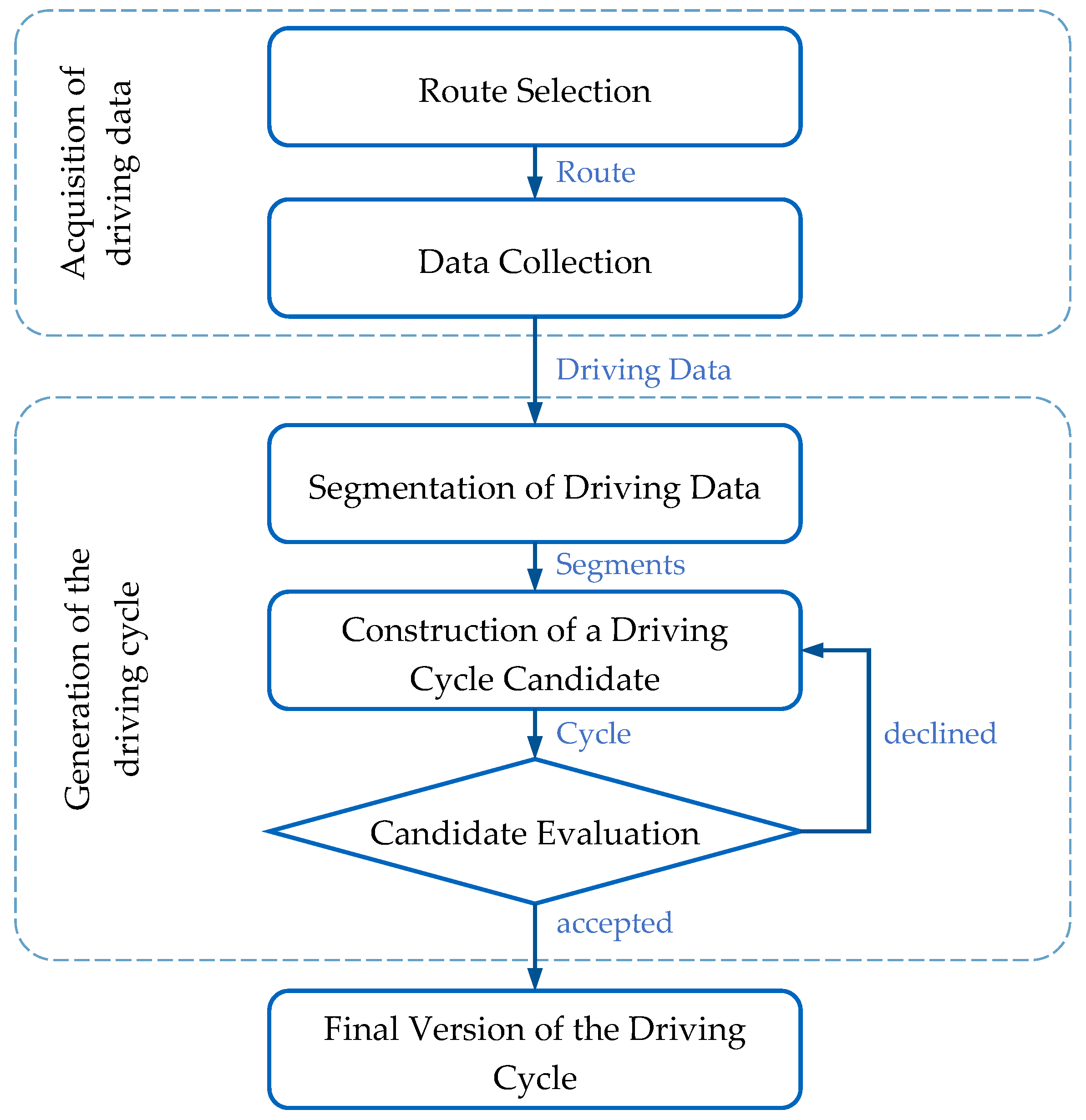
2.1. Development of Driving Cycles
2.2. Evaluation of Driving Style
2.3. Assessment Methods for Autonomous Vehicles
2.4. Research Gap
3. Development of the AVDC Tool
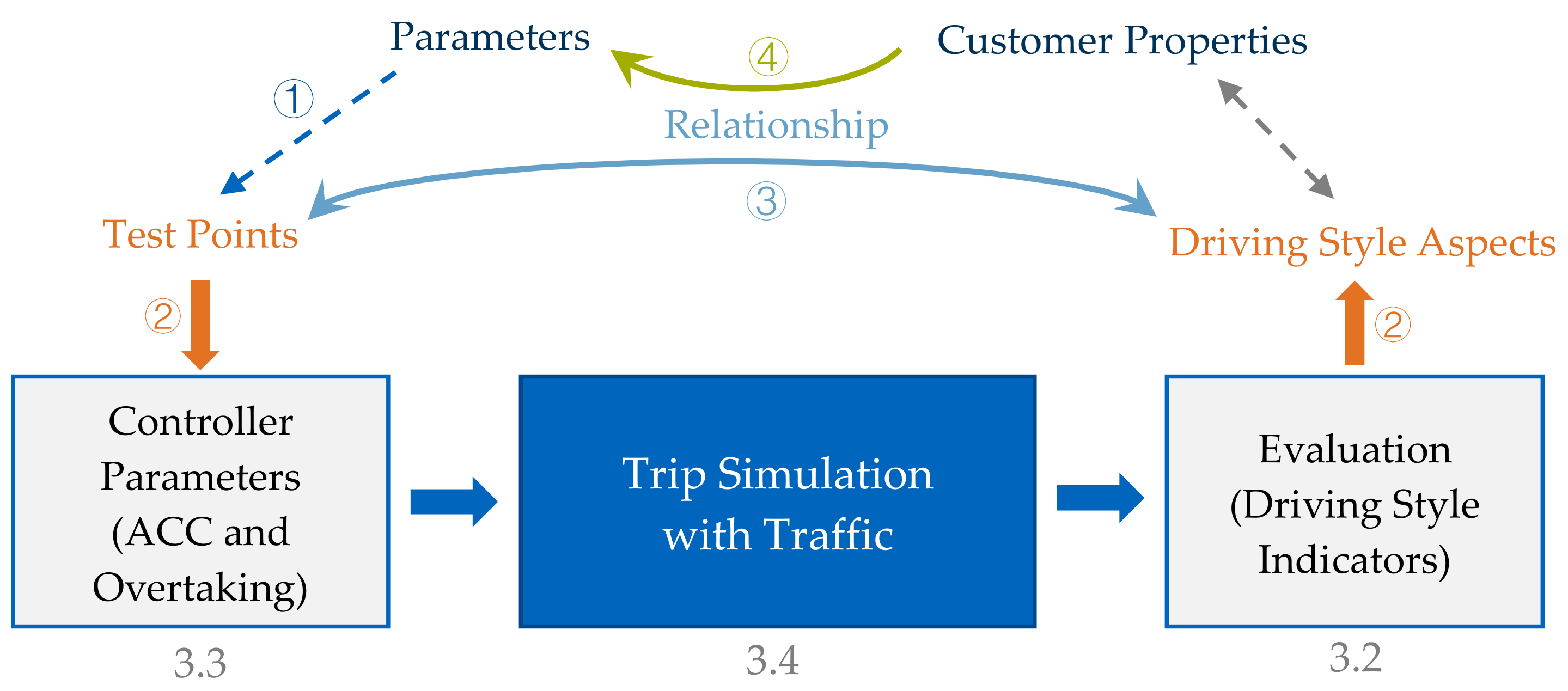
3.1. Concept
3.1.1. Basic Concepts and Assumptions
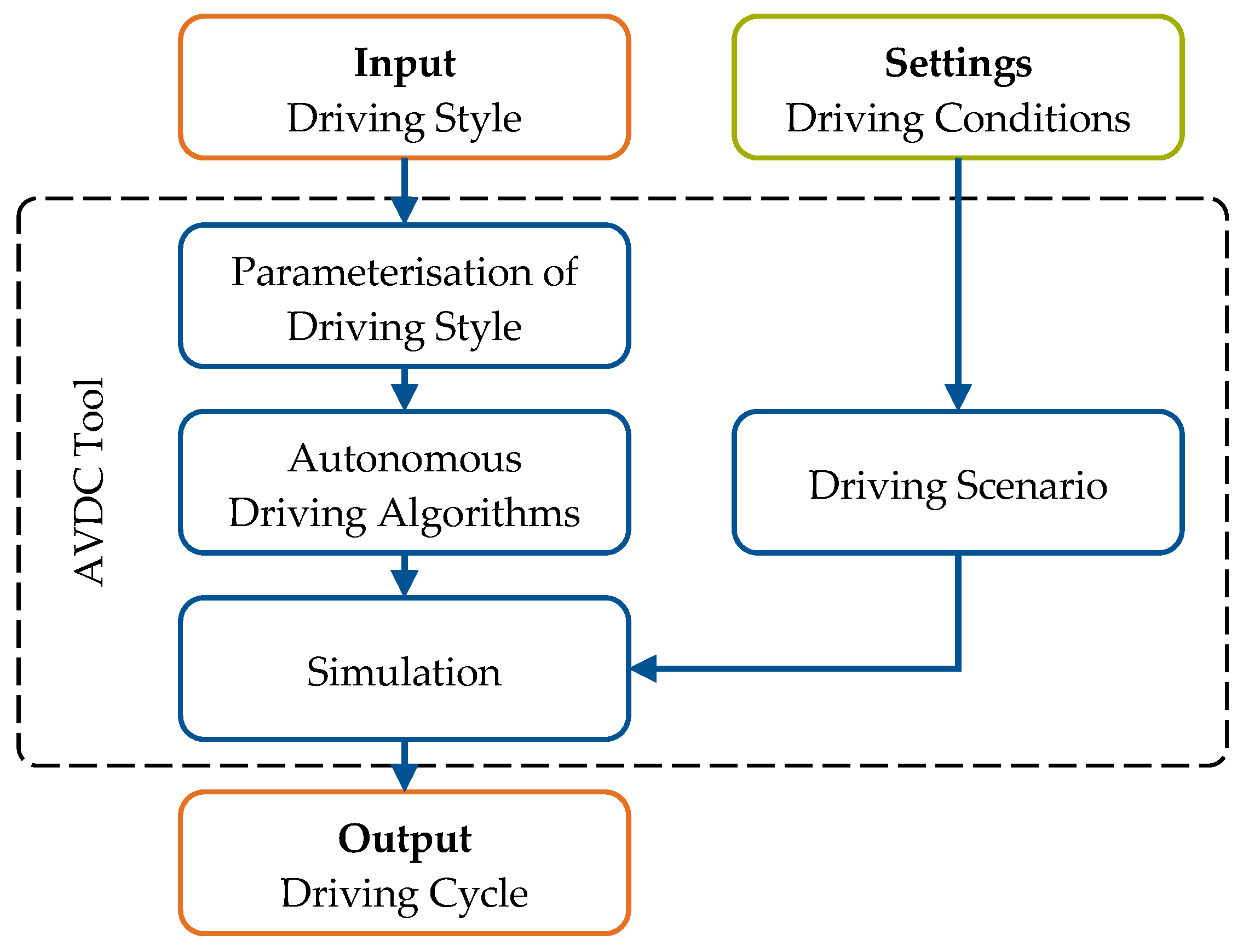
3.1.2. Structure of the Tool
3.2. Criterion for Driving Style
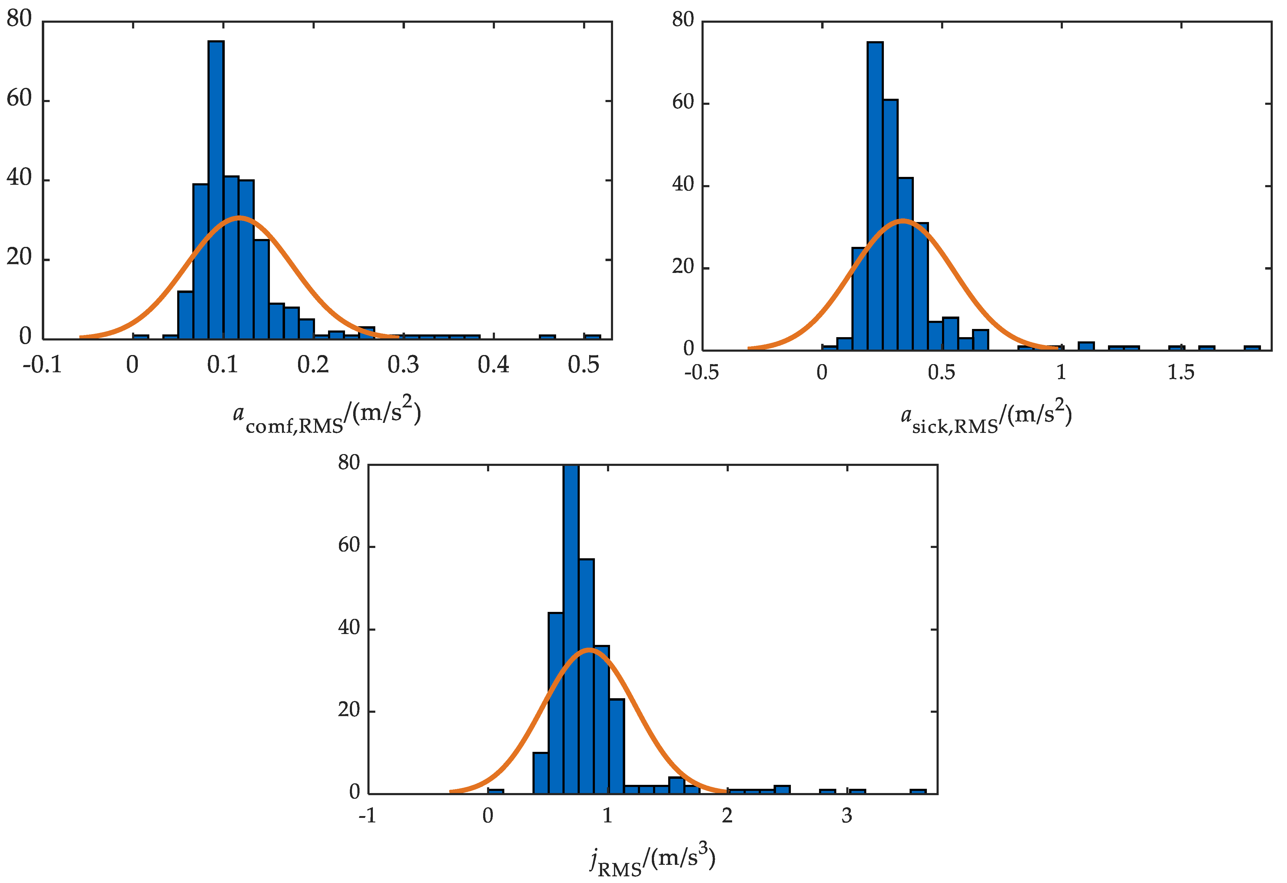
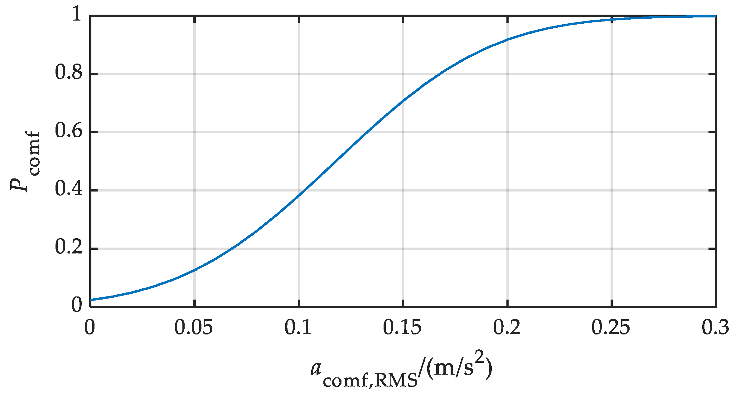
3.2.1. Comfort
- The driving segment was longer than 1 km.
- The speed signal was continuous and without sudden changes.
- The measured speeds from the OBD and the smartphone varied by a maximum of 5%.

| Indicator | Unit | ||
|---|---|---|---|
| m/s2 | 0.1177 | 0.0591 | |
| m/s2 | 0.3365 | 0.2160 | |
| m/s3 | 0.8438 | 0.3890 |

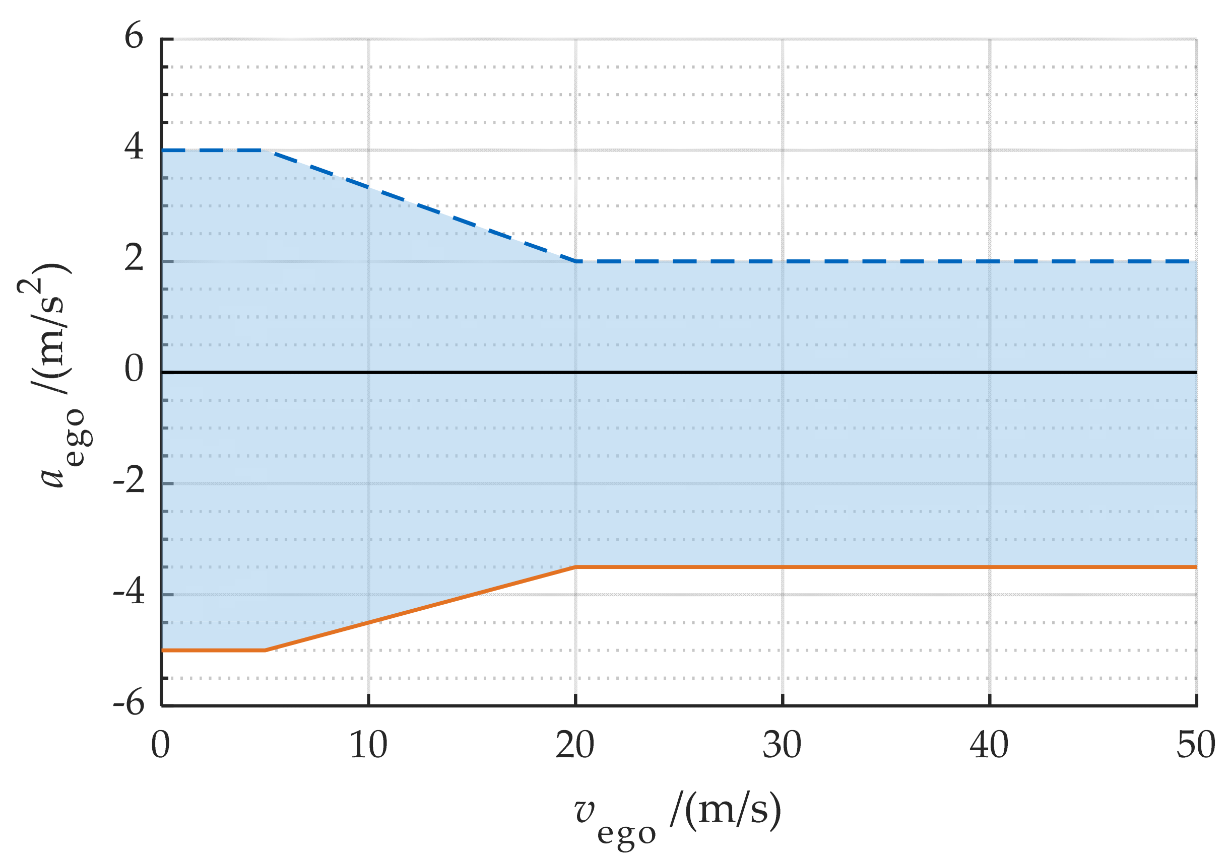
3.2.2. Safety
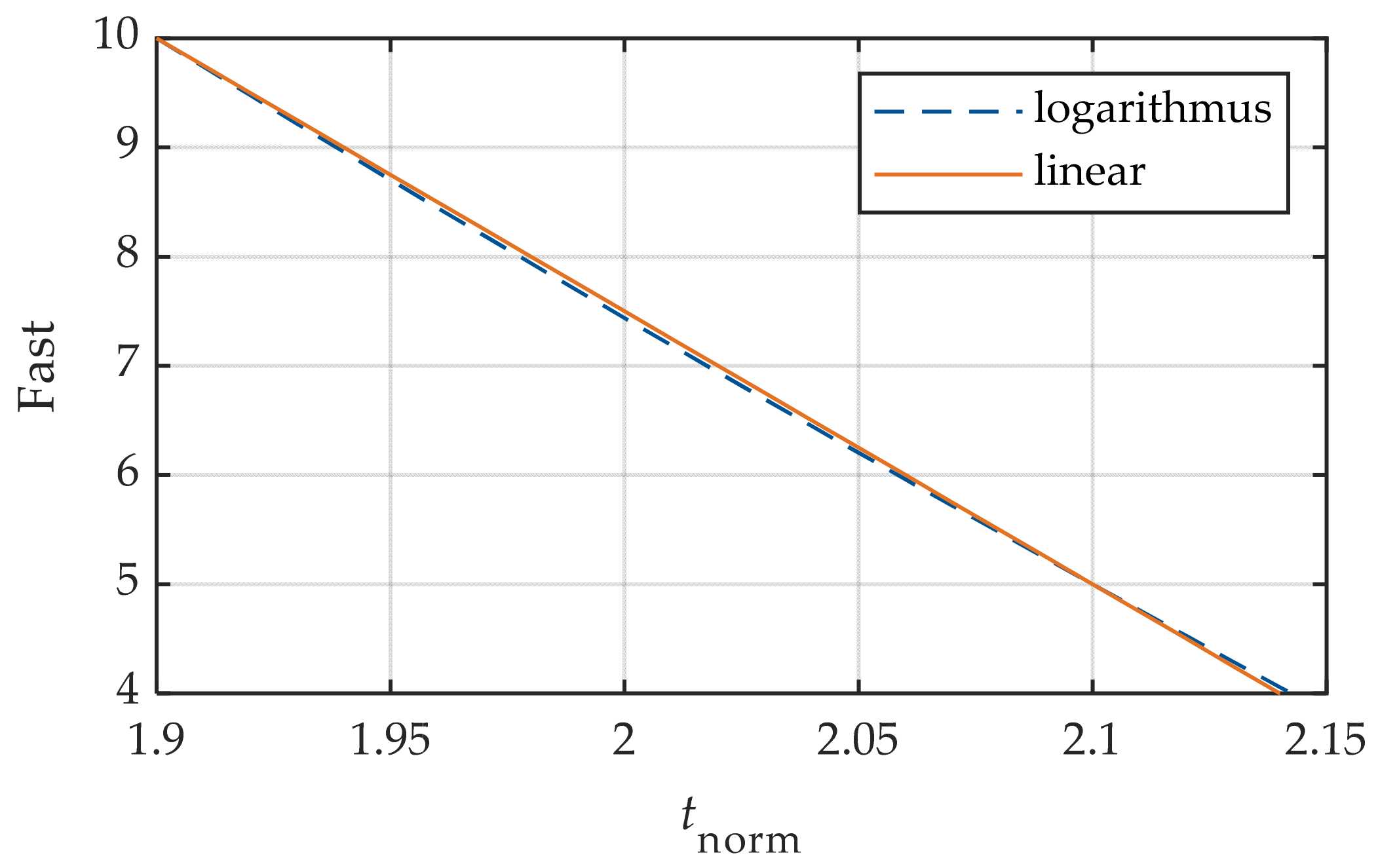
3.2.3. Swiftness
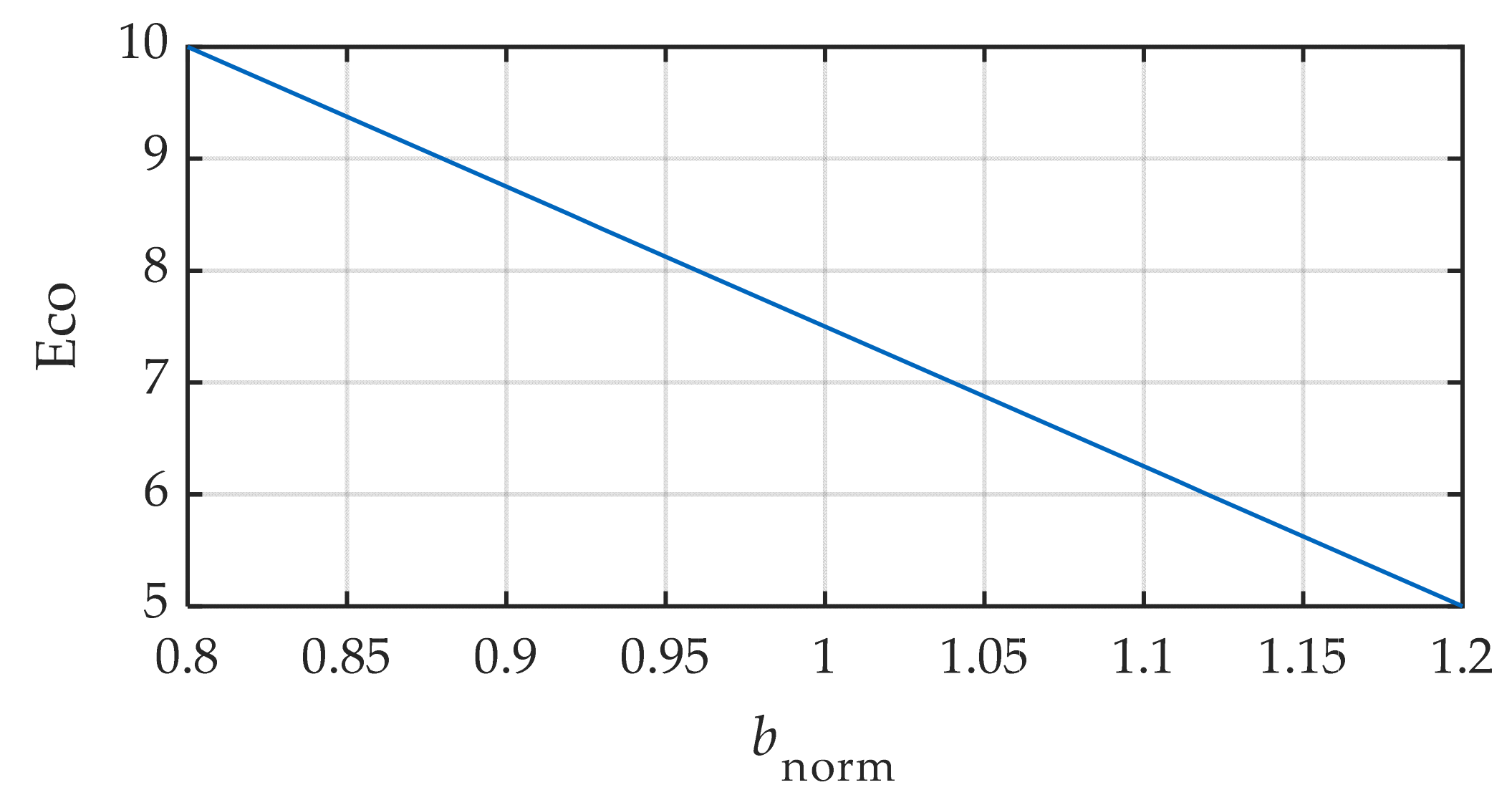
3.2.4. Economy
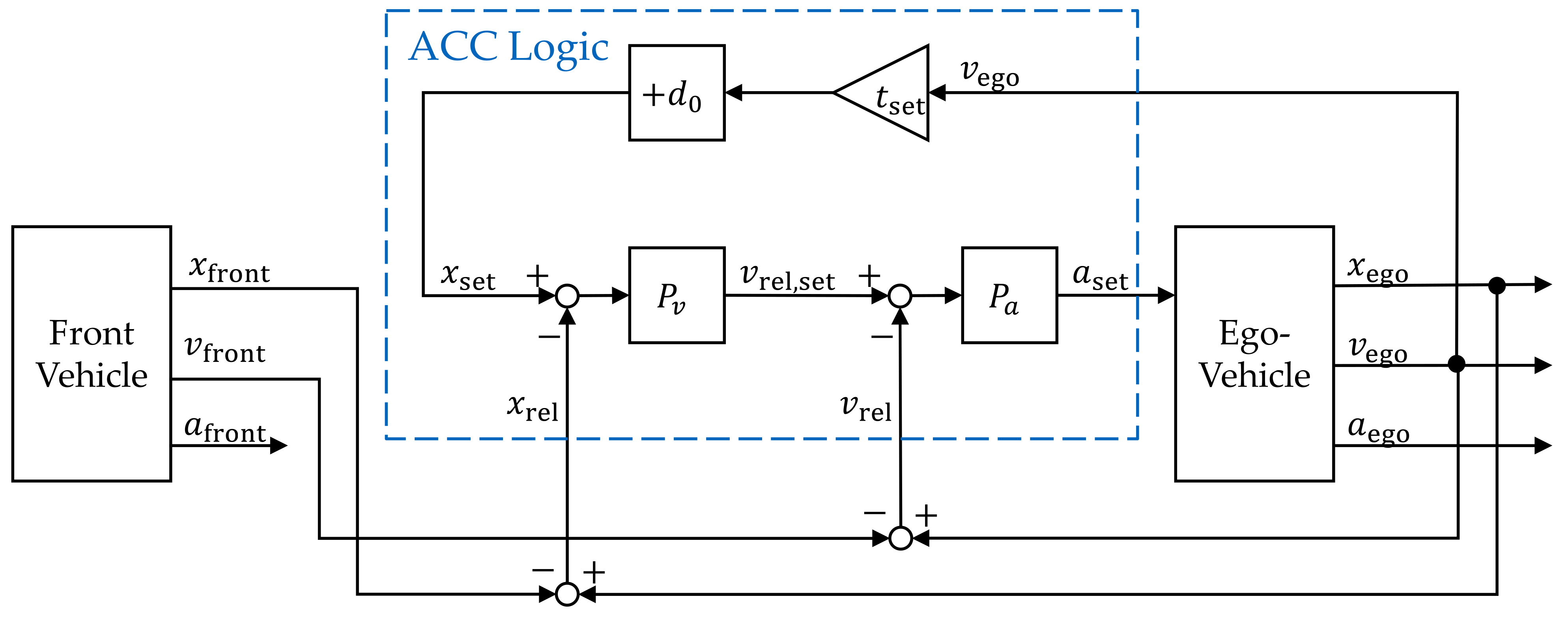
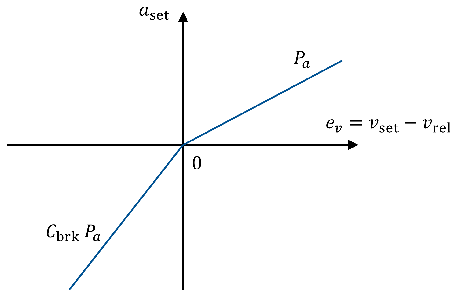
3.3. Autonomous Driving Algorithms
- The speed of front vehicle is lower than the set speed by more than the tolerance threshold :
- The estimated distance required for overtake is shorter than the available distance , where overtaking is allowed:
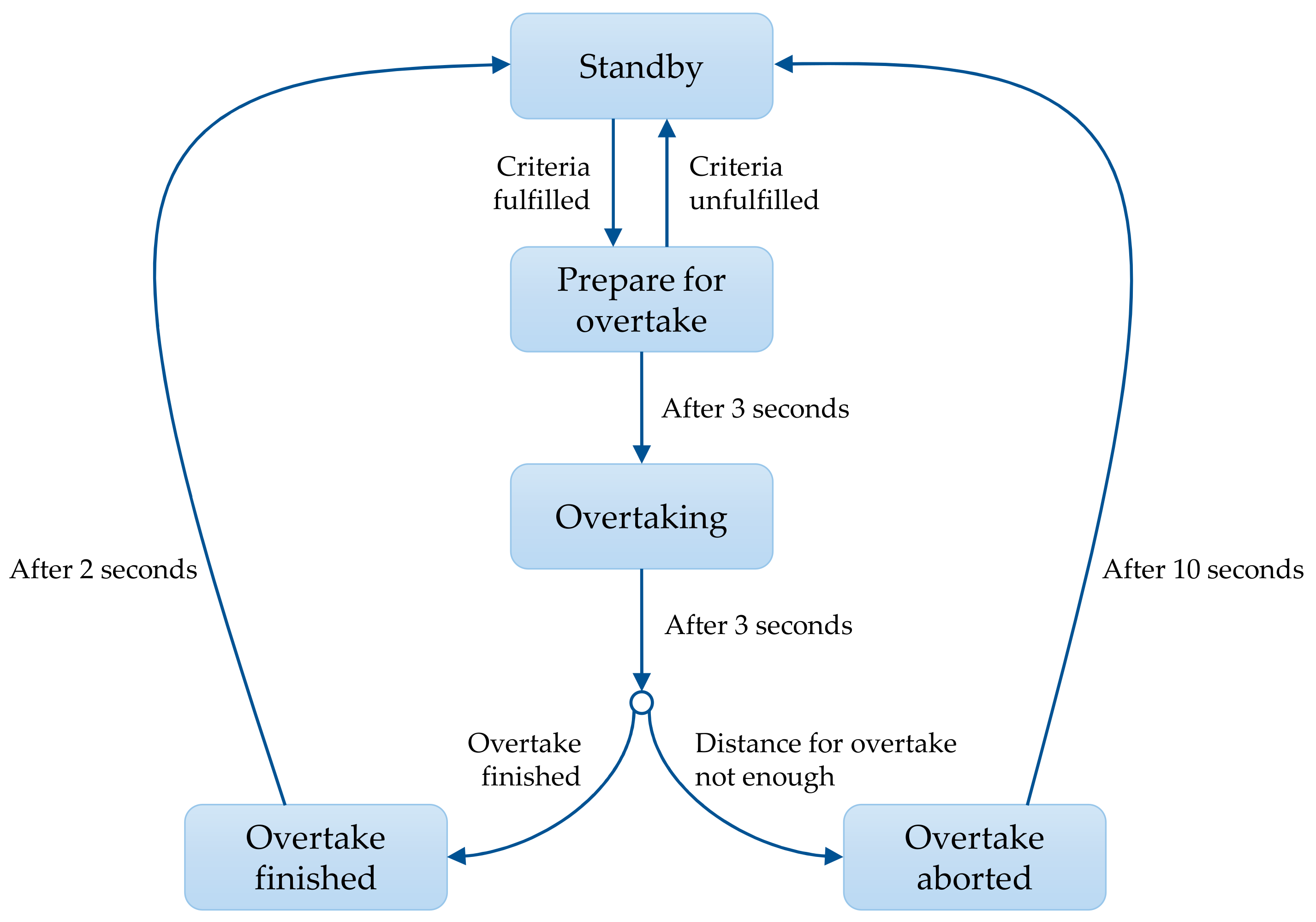
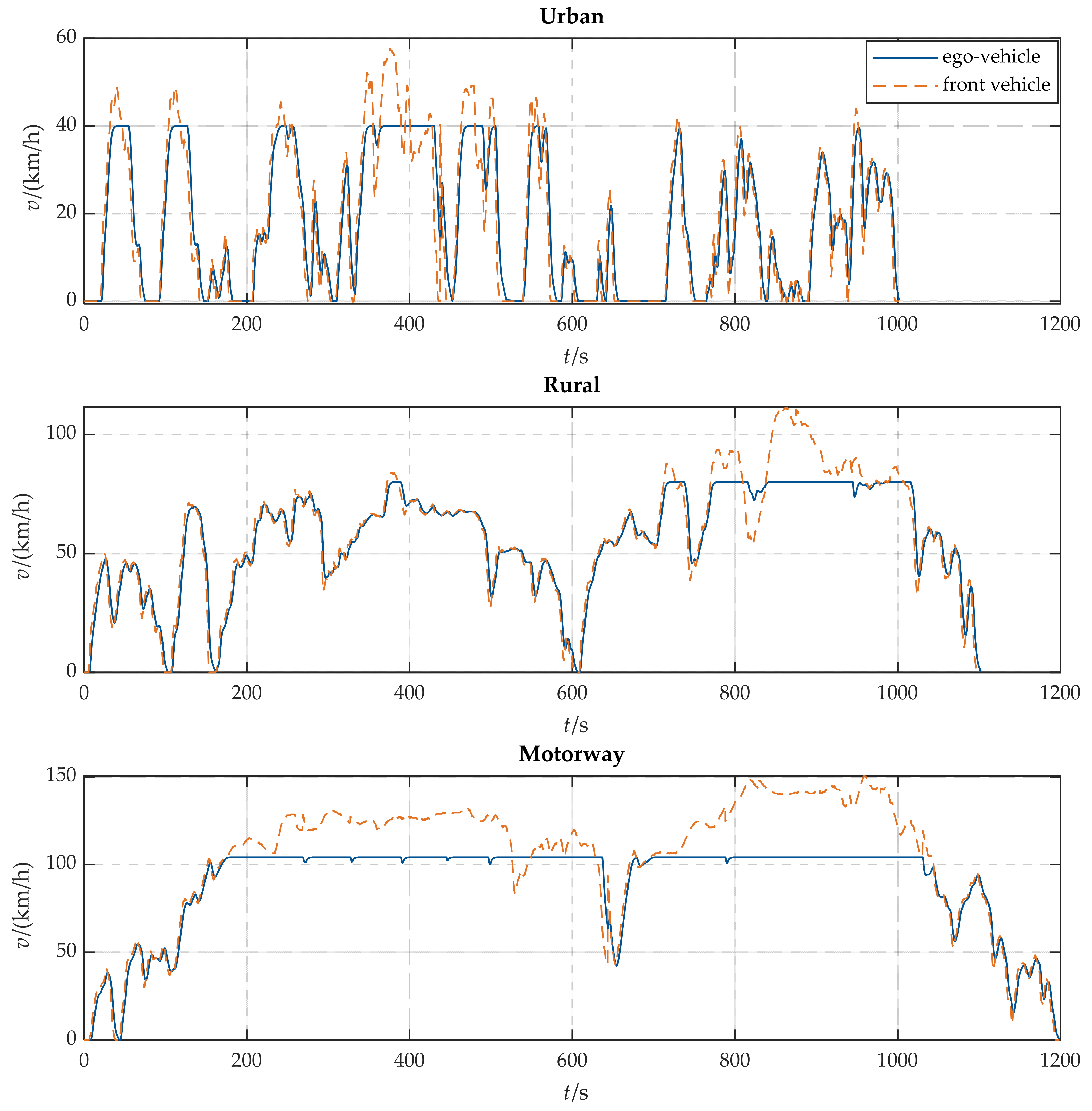
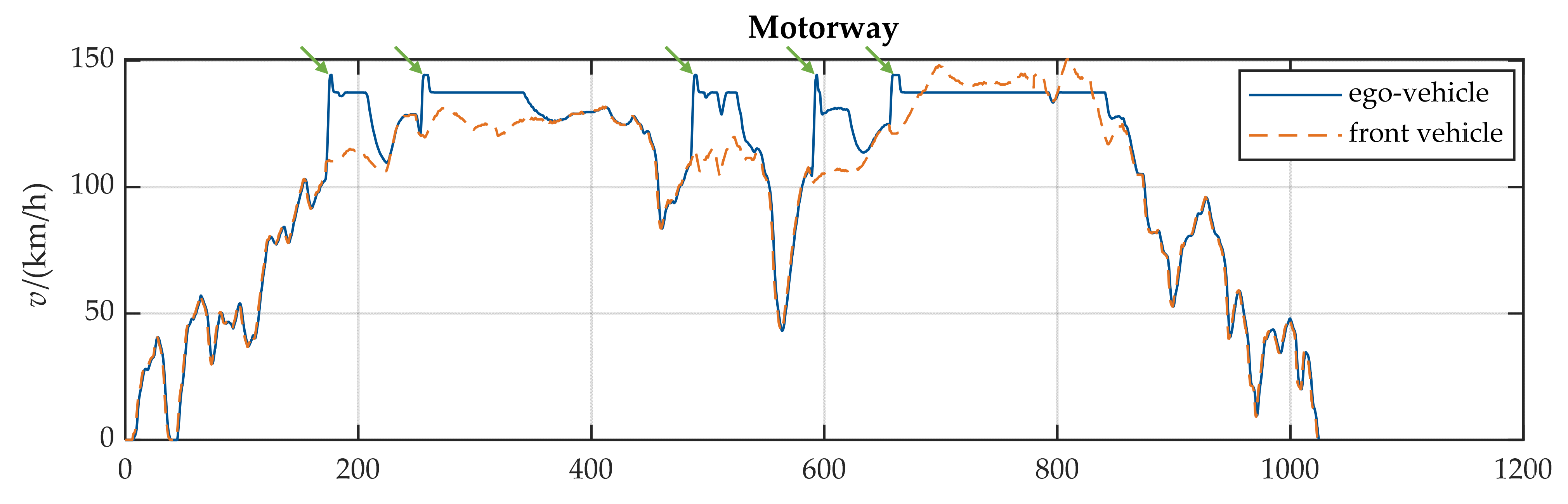
3.4. Driving Scenario
- The speed is within a window of 15 km/h for at least 20 s. This means that the vehicle travels at an approximately constant speed in the route section. If the speed changes rapidly, overtaking is inappropriate.
- The minimum speed in the window is higher than 30 km/h. The vehicle drives slowly when hindered by the driving environment, e.g., traffic lights or congestion. In these situations, overtaking is also inappropriate.
3.5. Parameterization of Driving Style
3.5.1. Definition of Setting Parameters
3.5.2. Design of the Experiment
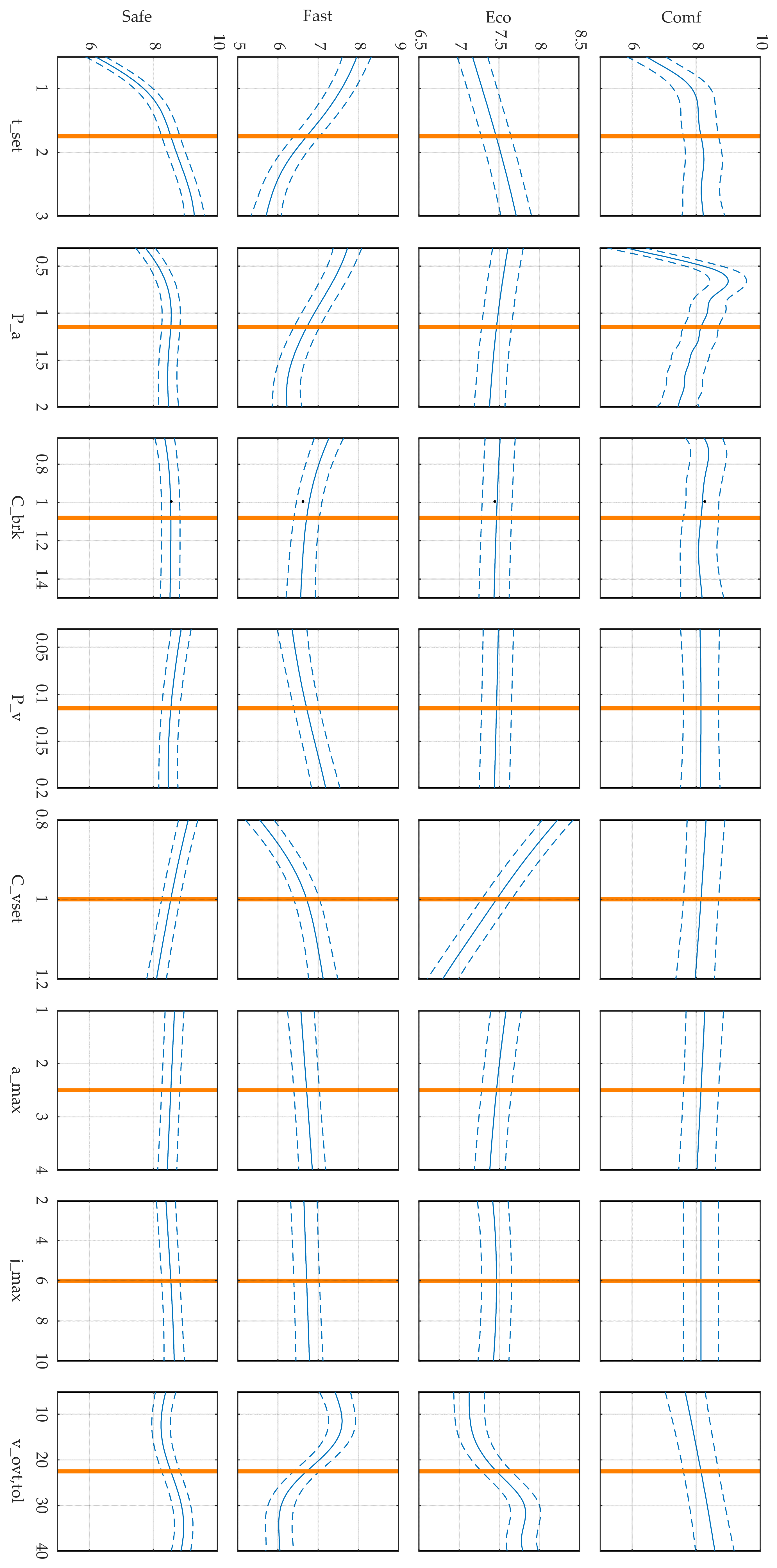
3.5.3. Modelling of Driving Style Aspects
3.5.4. Generation of the Parameter Set
4. Results
- Comfortable driving style with ,
- Safe driving style with ,
- Swift driving style with .
- —the duration of the driving cycle,
- —the average speed during the driving cycle,
- —the highest speed during the driving cycle,
- —the RMS value of acceleration during the driving cycle,
- —the RMS value of the jerk during the driving cycle,
- —the mean of the reciprocal of TTC during the driving cycle,
- —the number of vehicles overtaken during the driving cycle (if the ego vehicle is overtaken by traffic, the number is counted as negative).
- —the consumption of the drive cycle (in LDS of Tesla Model 3 with rear-wheel drive [53])
| Road Category | Driving Style | s | km/h | km/h | m/s2 | m/s3 | 1/s | - | kWh/100 km |
|---|---|---|---|---|---|---|---|---|---|
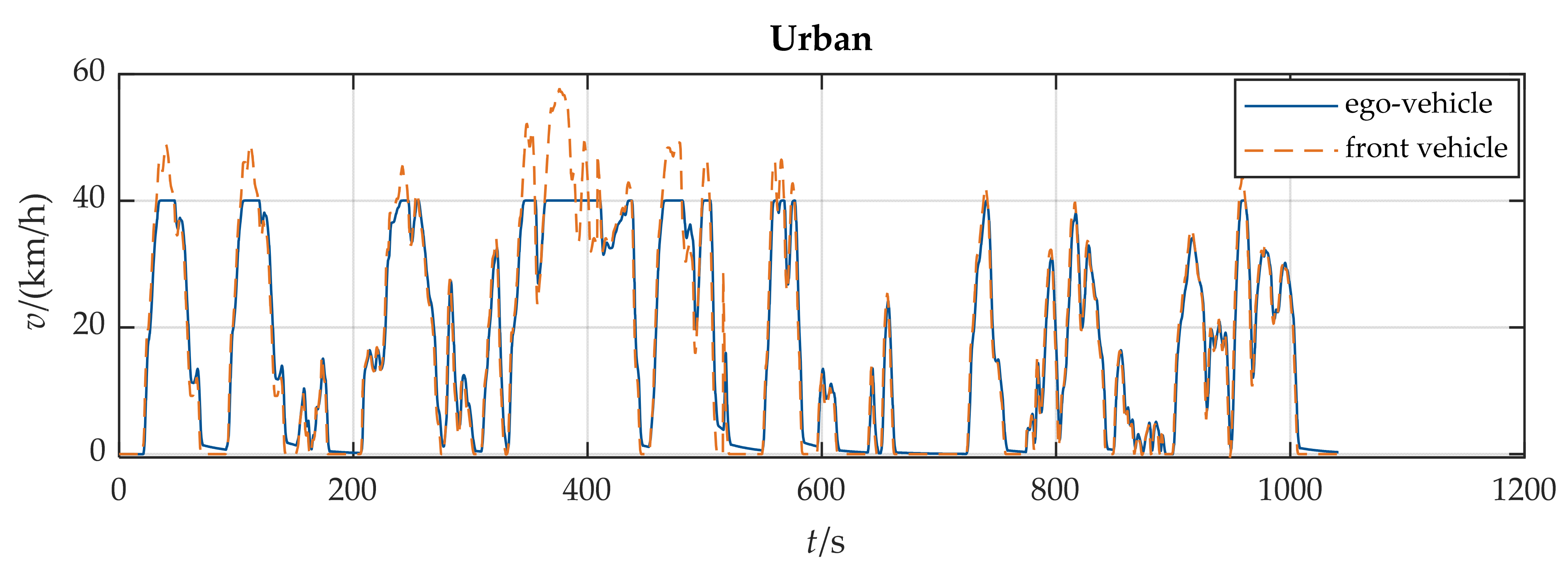
| urban | original | 986 | 17.8 | 57.7 | 0.80 | 0.95 | / | / | 14.56 |
| comfortable | 998 | 17.5 | 40.0 | 0.55 | 0.44 | 0.038 | −1 | 11.84 | |
| safe | 1006 | 17.3 | 40.0 | 0.68 | 0.78 | 0.013 | −2 | 12.55 | |
| swift | 986 | 17.8 | 50.0 | 0.75 | 0.86 | 0.084 | 0 | 13.97 | |
| rural | original | 1076 | 57.8 | 111.5 | 0.64 | 0.66 | / | / | 15.61 |
| comfortable | 1099 | 56.6 | 80.1 | 0.47 | 0.25 | 0.015 | −2 | 14.42 | |
| safe | 1108 | 56.1 | 80.1 | 0.56 | 0.46 | 0.006 | −3 | 14.71 | |
| swift | 986 | 63.0 | 105.0 | 0.75 | 1.16 | 0.053 | 9 | 17.20 | |
| motorway | original | 1063 | 100.1 | 150.4 | 0.56 | 0.66 | / | / | 24.44 |
| comfortable | 1195 | 89.0 | 104.1 | 0.39 | 0.25 | 0.007 | −13 | 20.13 | |
| safe | 1194 | 89.0 | 104.1 | 0.47 | 0.40 | 0.003 | −13 | 20.28 | |
| swift | 1023 | 103.9 | 144.3 | 0.66 | 0.63 | 0.025 | 4 | 21.16 |
5. Discussion
6. Conclusions
Author Contributions
Funding
Informed Consent Statement
Data Availability Statement
Conflicts of Interest
Appendix A. Response Models of the Parameters
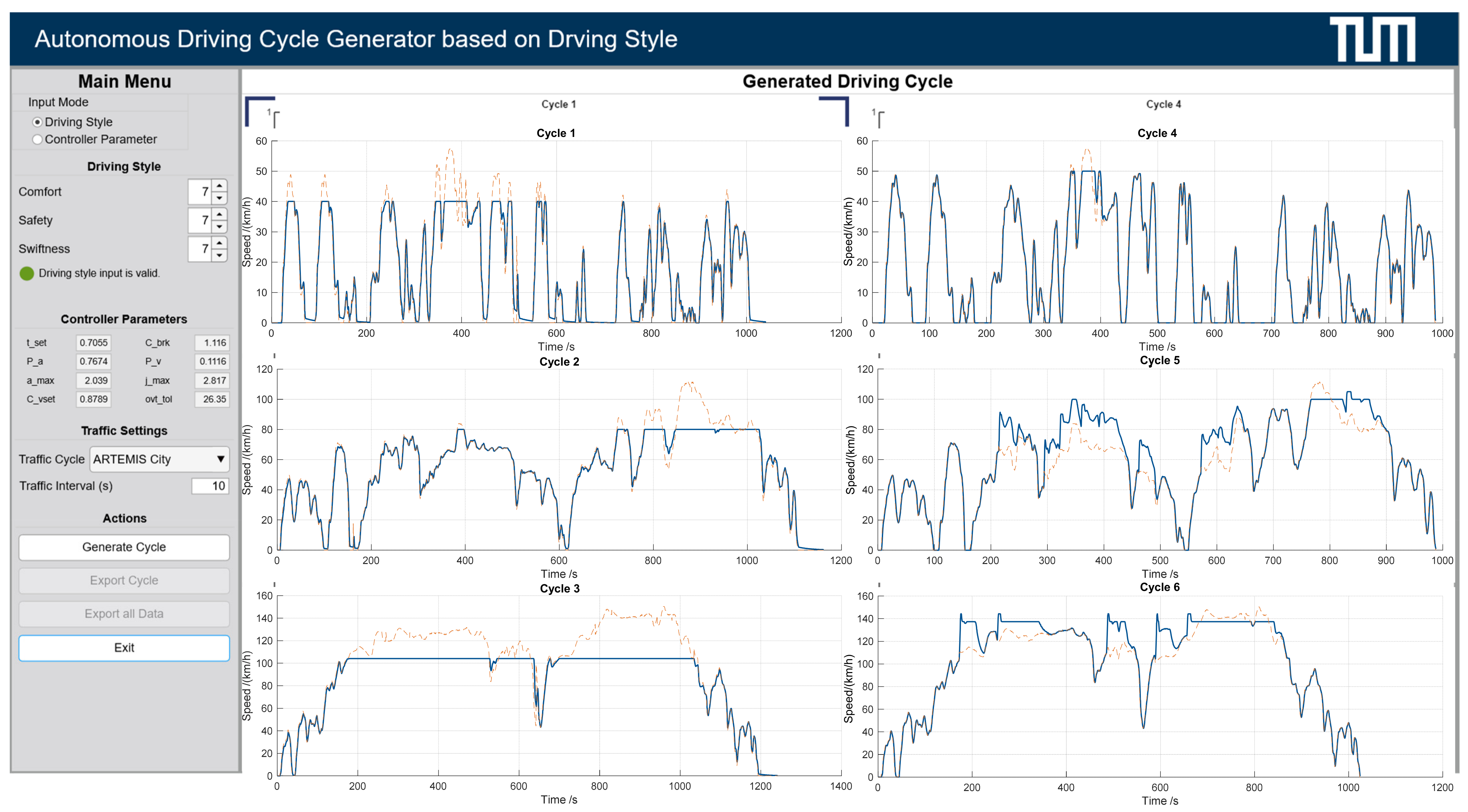
Appendix B. GUI of the AVDC Tool
References
- Yurtsever, E.; Lambert, J.; Carballo, A.; Takeda, K. A Survey of Autonomous Driving: Common Practices and Emerging Technologies. IEEE Access 2020, 8, 58443–58469. [Google Scholar] [CrossRef]
- Mallozzi, P.; Pelliccione, P.; Knauss, A.; Berger, C.; Mohammadiha, N. Autonomous Vehicles: State of the Art, Future Trends, and Challenges. In Automotive Systems and Software Engineering; Dajsuren, Y., van den Brand, M., Eds.; Springer: Berlin/Heidelberg, Germany, 2019; pp. 347–367. ISBN 978-3-030-12156-3. [Google Scholar]
- Shreyas, V.; Bharadwaj, S.N.; Srinidhi, S.; Ankith, K.U.; Rajendra, A.B. Self-driving Cars: An Overview of Various Autonomous Driving Systems. In Advances in Data and Information Sciences: Proceedings of ICDIS 2019; Kolhe, M., Tiwari, S., Trivedi, M.C., Mishra, K.K., Eds.; Springer: Singapore, 2020; pp. 361–371. ISBN 978-981-15-0693-2. [Google Scholar]
- Koenig, A.; Schockenhoff, F.; Koch, A.; Lienkamp, M. Concept Design Optimization of Autonomous and Electric Vehicles. In Proceedings of the 2019 8th International Conference on Power Science and Engineering (ICPSE), Dublin, Ireland, 2–4 December 2019; IEEE: New York, NY, USA, 2019; pp. 44–49, ISBN 978-1-7281-6081-8. [Google Scholar]
- Regulation (EU) 2019/631 of the European Parliament and of the Council of 17 April 2019 Setting CO2 Emission Performance Standards for New Passenger Cars and for New Light Commercial Vehicles, and Repealing REGULATIONS (EC) No 443/2009 and (EU) No 510/2011; Publications Office of the European Union: Luxembourg, 2019.
- Kim, M.-J.; Peng, H. Power management and design optimization of fuel cell/battery hybrid vehicles. J. Power Sources 2007, 165, 819–832. [Google Scholar] [CrossRef] [Green Version]
- Carraro, E.; Morandin, M.; Bianchi, N. Traction PMASR Motor Optimization According to a Given Driving Cycle. IEEE Trans. Ind. Appl. 2016, 52, 209–216. [Google Scholar] [CrossRef]
- Barlow, T.J.; Latham, S.; McCrae, I.S.; Boulter, P.G. A Reference Book of Driving Cycles for Use in the Measurement of Road Vehicle Emissions; Version 3; TRL Limited: Wokingham, UK, 2009. [Google Scholar]
- Duan, X.; Schockenhoff, F. Autonomous Vehicle Driving Cycle Tool. Available online: https://github.com/TUMFTM/AV_Driving_Cycles (accessed on 9 April 2022).
- The MathWorks, Inc. Simulink—Simulation and Model-Based Design. Available online: https://ww2.mathworks.cn/en/products/simulink.html (accessed on 9 April 2022).
- SAE International. SAE Levels of Driving Automation™ Refined for Clarity and International Audience. Available online: https://www.sae.org/blog/sae-j3016-update (accessed on 14 March 2022).
- Zhang, X.; Zhao, D.-J.; Shen, J.-M. A Synthesis of Methodologies and Practices for Developing Driving Cycles. Energy Procedia 2012, 16, 1868–1873. [Google Scholar] [CrossRef] [Green Version]
- Tutuianu, M.; Bonnel, P.; Ciuffo, B.; Haniu, T.; Ichikawa, N.; Marotta, A.; Pavlovic, J.; Steven, H. Development of the World-wide harmonized Light duty Test Cycle (WLTC) and a possible pathway for its introduction in the European legislation. Transp. Res. Part D Transp. Environ. 2015, 40, 61–75. [Google Scholar] [CrossRef]
- GB/T 38146.1-2019; China Automotive Test Cycle—Part 1: Light-Duty Vehicles. China National Standardization Administration: Beijing, China, 2019.
- Yang, Z. Factsheet: Japan Light-Duty Vehicle Efficiency Standards. Available online: https://theicct.org/sites/default/files/Japan_PVstds-facts_jan2015.pdf (accessed on 5 December 2021).
- Tong, H.Y.; Hung, W.T. A Framework for Developing Driving Cycles with On-Road Driving Data. Transp. Rev. 2010, 30, 589–615. [Google Scholar] [CrossRef]
- Galgamuwa, U.; Perera, L.; Bandara, S. Developing a General Methodology for Driving Cycle Construction: Comparison of Various Established Driving Cycles in the World to Propose a General Approach. J. Transp. Technol. 2015, 5, 191–203. [Google Scholar] [CrossRef] [Green Version]
- Zähringer, M.; Kalt, S.; Lienkamp, M. Compressed Driving Cycles Using Markov Chains for Vehicle Powertrain Design. World Electr. Veh. J. 2020, 11, 52. [Google Scholar] [CrossRef]
- Elander, J.; West, R.; French, D. Behavioral correlates of individual differences in road-traffic crash risk: An examination method and findings. Psychol. Bull. 1993, 113, 279–294. [Google Scholar] [CrossRef]
- Sagberg, F.; Selpi; Piccinini, G.F.B.; Engström, J. A Review of Research on Driving Styles and Road Safety. Hum. Factors 2015, 57, 1248–1275. [Google Scholar] [CrossRef]
- Eboli, L.; Mazzulla, G.; Pungillo, G. How drivers’ characteristics can affect driving style. Transp. Res. Procedia 2017, 27, 945–952. [Google Scholar] [CrossRef]
- Gurusinghe, G.S.; Nakatsuji, T.; Azuta, Y.; Ranjitkar, P.; Tanaboriboon, Y. Multiple Car-Following Data with Real-Time Kinematic Global Positioning System. Transp. Res. Rec. 2002, 1802, 166–180. [Google Scholar] [CrossRef]
- Sun, P.; Wang, X.; Zhu, M. Modeling Car-Following Behavior on Freeways Considering Driving Style. J. Transp. Eng. Part A Syst. 2021, 147, 4021083. [Google Scholar] [CrossRef]
- van Mierlo, J.; Maggetto, G.; van de Burgwal, E.; Gense, R. Driving style and traffic measures-influence on vehicle emissions and fuel consumption. Proc. Inst. Mech. Eng. Part D J. Automob. Eng. 2004, 218, 43–50. [Google Scholar] [CrossRef]
- Felipe, J.; Amarillo, J.C.; Naranjo, J.E.; Serradilla, F.; Diaz, A. Energy Consumption Estimation in Electric Vehicles Considering Driving Style. In Proceedings of the 2015 IEEE 18th International Conference on Intelligent Transportation Systems—(ITSC 2015), Gran Canaria, Spain, 15–18 September 2015; IEEE: New York, NY, USA, 2015; pp. 101–106, ISBN 978-1-4673-6596-3. [Google Scholar]
- Berry, I.M. The Effects of Driving Style and Vehicle Performance on the Real-World Fuel Consumption of U.S. Light-Duty Vehicles. Master’s Thesis, Massachusetts Institute of Technology, Cambridge, MA, USA, 2010. [Google Scholar]
- Elbanhawi, M.; Simic, M.; Jazar, R. In the Passenger Seat: Investigating Ride Comfort Measures in Autonomous Cars. IEEE Intell. Transport. Syst. Mag. 2015, 7, 4–17. [Google Scholar] [CrossRef]
- Kottenhoff, K. Driving Styles and the Effect on Passengers: Developing Ride Comfort Indicators. 2016. Available online: http://www.diva-portal.org/smash/get/diva2:898005/FULLTEXT01.pdf (accessed on 26 August 2021).
- Hashimoto, T.; Yanagisawa, H. Risk Feeling Index of Autonomous Vehicle Behavior. In Proceedings of the 6th International Symposium on Affective Science and Engineering (ISASE 2020), Tokyo, Japan, 15–16 March 2020; pp. 1–4. [Google Scholar] [CrossRef]
- Qiao, X.; Zheng, L.; Li, Y.; Ren, Y.; Zhang, Z.; Zhang, Z.; Qiu, L. Characterization of the Driving Style by State–Action Semantic Plane Based on the Bayesian Nonparametric Approach. Appl. Sci. 2021, 11, 7857. [Google Scholar] [CrossRef]
- Murphey, Y.L.; Milton, R.; Kiliaris, L. Driver’s style classification using jerk analysis. In Proceedings of the 2009 IEEE Workshop on Computational Intelligence in Vehicles and Vehicular Systems (CIVVS 2009), Nashville, TN, USA, 30 March–2 April 2009; IEEE: Piscataway, NJ, USA, 2009; pp. 23–28, ISBN 978-1-4244-2770-3. [Google Scholar]
- Dörr, D.; Grabengiesser, D.; Gauterin, F. Online driving style recognition using fuzzy logic. In Proceedings of the 17th International IEEE Conference on Intelligent Transportation Systems (ITSC), Qingdao, China, 10 August–10 November 2014; IEEE: New York, NY, USA, 2014; pp. 1021–1026, ISBN 978-1-4799-6078-1. [Google Scholar]
- Karjanto, J.; Yusof, N.M.; Terken, J.; Delbressine, F.; Hassan, M.Z.; Rauterberg, M. Simulating autonomous driving styles: Accelerations for three road profiles. MATEC Web Conf. 2017, 90, 1005. [Google Scholar] [CrossRef] [Green Version]
- Schockenhoff, F.; Nehse, H.; Lienkamp, M. Maneuver-Based Objectification of User Comfort Affecting Aspects of Driving Style of Autonomous Vehicle Concepts. Appl. Sci. 2020, 10, 3946. [Google Scholar] [CrossRef]
- Jachimczyk, B.; Dziak, D.; Czapla, J.; Damps, P.; Kulesza, W.J. IoT On-Board System for Driving Style Assessment. Sensors 2018, 18, 1233. [Google Scholar] [CrossRef] [Green Version]
- Kondoh, T.; Yamamura, T.; Kitazaki, S.; Kuge, N.; Boer, E.R. Identification of Visual Cues and Quantification of Drivers’ Perception of Proximity Risk to the Lead Vehicle in Car-Following Situations. JMTL 2008, 1, 170–180. [Google Scholar] [CrossRef] [Green Version]
- Lu, G.; Cheng, B.; Lin, Q.; Wang, Y. Quantitative indicator of homeostatic risk perception in car following. Saf. Sci. 2012, 50, 1898–1905. [Google Scholar] [CrossRef]
- Zhang, X.; Lu, G.; Cheng, B. Parameters Calibration for Car-Following Model Based Desired Safety Margin. In Proceedings of the International Conference on Optoelectronics and Image Processing (ICOIP), Haiko, China, 11 November–11 December 2010; IEEE: New York, NY, USA, 2010; pp. 97–100, ISBN 978-1-4244-8683-0. [Google Scholar]
- Griesche, S.; Nicolay, E.; Assmann, D.; Dotzauer, M.; Käthner, D. Should my car drive as I do? What kind of driving style do drivers prefer for the design of automated driving functions? In Proceedings of the 17 Braunschweiger Symposium AAET, Braunschweig, Germany, 9–11 February 2016. [Google Scholar]
- Scherer, S.; Dettmann, A.; Hartwich, F.; Pech, T.; Bullinger, A.C.; Wanielik, G. How the driver wants to be driven—Modelling driving styles in highly automated driving. In Proceedings of the 7. Tagung Fahrerassistenz, Munich, Germany, 25–26 November 2015. [Google Scholar]
- Xue, Q.; Wang, K.; Lu, J.J.; Liu, Y. Rapid Driving Style Recognition in Car-Following Using Machine Learning and Vehicle Trajectory Data. J. Adv. Transp. 2019, 2019, 9085238. [Google Scholar] [CrossRef] [Green Version]
- Mersky, A.C.; Samaras, C. Fuel economy testing of autonomous vehicles. Transp. Res. Part C Emerg. Technol. 2016, 65, 31–48. [Google Scholar] [CrossRef]
- Roshdi, M.; Nayeer, N.; Elmahgiubi, M.; Agrawal, A.; Garcia, D.E. A Unified Evaluation Framework for Autonomous Driving Vehicles. In Proceedings of the 2020 IEEE Intelligent Vehicles Symposium (IV), Las Vegas, NV, USA, 19 October–13 November 2020; IEEE: New York, NY, USA, 2020; pp. 1277–1282, ISBN 978-1-7281-6673-5. [Google Scholar]
- Costandoiu, A.; Leba, M. Convergence of V2X communication systems and next generation networks. IOP Conf. Ser. Mater. Sci. Eng. 2019, 477, 12052. [Google Scholar] [CrossRef]
- Schockenhoff, F.; König, A.; Koch, A.; Lienkamp, M. Customer-Relevant Properties of Autonomous Vehicle Concepts. Procedia CIRP 2020, 91, 55–60. [Google Scholar] [CrossRef]
- Bae, I.; Moon, J.; Seo, J. Toward a Comfortable Driving Experience for a Self-Driving Shuttle Bus. Electronics 2019, 8, 943. [Google Scholar] [CrossRef] [Green Version]
- Bellem, H. Comfort in Automated Driving: Analysis of Driving Style Preference in Automated Driving. Ph.D. Thesis, Technischen Universität Chemnitz, Chemnitz, Germany, 2018. [Google Scholar]
- Bellem, H.; Schönenberg, T.; Krems, J.F.; Schrauf, M. Objective metrics of comfort: Developing a driving style for highly automated vehicles. Transp. Res. Part F Traffic Psychol. Behav. 2016, 41, 45–54. [Google Scholar] [CrossRef]
- 13.160 (ISO 2631-1:1997); Mechanical Vibration and Shock—Evaluation of Human Exposure to Whole-Body Vibration—Part 1: General Requirements. International Organization for Standardization: Geneva, Switzerland, 1997.
- 13.160 (ISO 2631-1:1997/AMD 1:2010); Mechanical Vibration and Shock—Evaluation of Human Exposure to Whole-Body Vibration—Part 1: General Requirements—Amendment 1. International Organization for Standardization: Geneva, Switzerland, 2010.
- Wassiliadis, N.; Steinsträter, M.; Schreiber, M.; Rosner, P.; Nicoletti, L.; Schmid, F.; Ank, M.; Teichert, O.; Wildfeuer, L.; Schneider, J.; et al. Quantifying the state of the art of electric powertrains in battery electric vehicles: Range, efficiency, and lifetime from component to system level of the Volkswagen ID.3. eTransportation 2022, 12, 100167. [Google Scholar] [CrossRef]
- Langer, L. Ableitung Konzeptbestimmender Technischer Werte Autonomer Fahrzeuge anhand Einer Marktanalyse; Semesterarbeit; Lehrstuhl für Fahrzeugtechnik: Munich, Germany, 2021. [Google Scholar]
- König, A.; Nicoletti, L.; Kalt, S.; Müller, K.; Koch, A.; Lienkamp, M. An Open-Source Modular Quasi-Static Longitudinal Simulation for Full Electric Vehicles. In Proceedings of the 2020 Fifteenth International Conference on Ecological Vehicles and Renewable Energies (EVER), Monte-Carlo, Monaco, 10–12 September 2020; IEEE: New York, NY, USA, 2020; pp. 1–9, ISBN 978-1-7281-5641-5. [Google Scholar]
- Winner, H.; Hakuli, S.; Lotz, F.; Singer, C. Handbuch Fahrerassistenzsysteme: Grundlagen, Komponenten und Systeme für Aktive Sicherheit und Komfort; 3. Auflage; Springer Vieweg: Wiesbaden, Germany, 2015; ISBN 978-3-658-05734-3. [Google Scholar]
- 03.220.20 (ISO 15622:2018); Intelligent Transport Systems—Adaptive Cruise Control Systems—Performance Requirements and Test Procedures. International Organization for Standardization: Geneva, Switzerland, 2018.
- André, M.; Keller, M.; Sjödin, Å.; Gadrat, M.; Crae, I.M.; Dilara, P. The ARTEMIS European Tools for Estimating the Transport Pollutant Emissions. 2009. Available online: https://www3.epa.gov/ttnchie1/conference/ei18/session6/andre.pdf (accessed on 19 July 2021).
- André, M. The ARTEMIS European driving cycles for measuring car pollutant emissions. Sci. Total Environ. 2004, 334–335, 73–84. [Google Scholar] [CrossRef]
- The MathWorks, Inc. Model-Based Calibration Toolbox. Available online: https://ww2.mathworks.cn/en/products/mbc.html (accessed on 19 April 2022).
- Hartwich, F.; Beggiato, M.; Dettmann, A.; Krems, J. Drive Me Comfortable. Customized Automated Driving Styles for Younger and Older Drivers. In Der Fahrer im 21. Jahrhundert: Fahrer, Fahrerunterstützung und Bedienbarkeit; Proceedings of the 8. VDI-Tagung, Braunschweig, Germany, 10–11 November 2015; VDI-Verlag GmbH: Düsseldorf, Germany, 2015; pp. 271–283. ISBN 978-3-18-092264-5. [Google Scholar]


| Road Category | Highest Speed in km/h |
|---|---|
| Urban | |
| Rural | |
| Motorway |
| Parameter | Unit | Min. Value | Ref. Value | Max. Value | Description |
|---|---|---|---|---|---|
| s | 0.5 | 2 | 3 | Set time headways of ACC | |
| - | 0.3 | 0.7 | 2 | P-coefficient of speed controller | |
| - | 0.66 | 1 | 1.5 | Coefficient for deceleration | |
| - | 0.03 | 0.07 | 0.2 | P-coefficient of distance controller | |
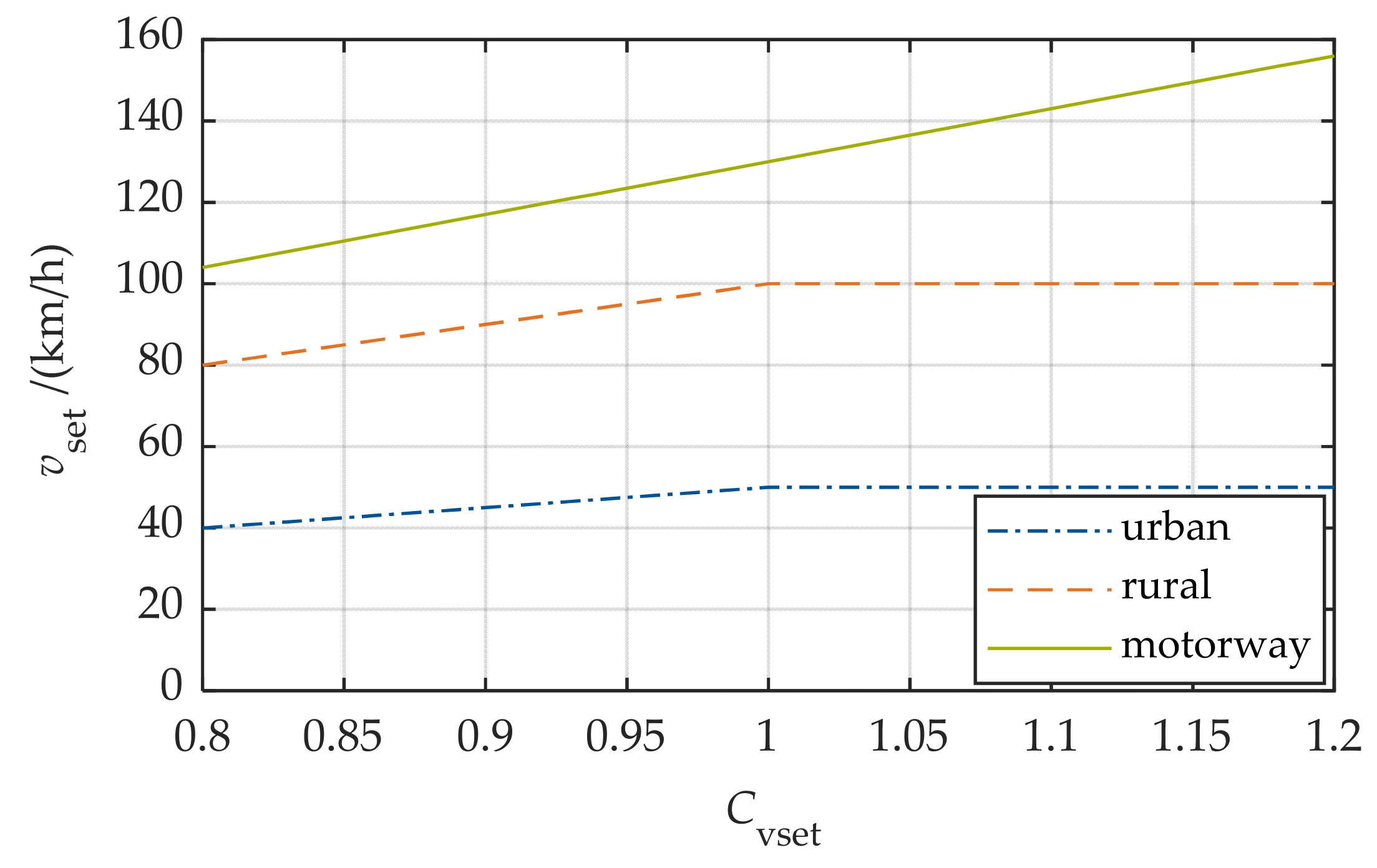
| - | 0.8 | 1 | 1.2 | Coefficient for set speed | |
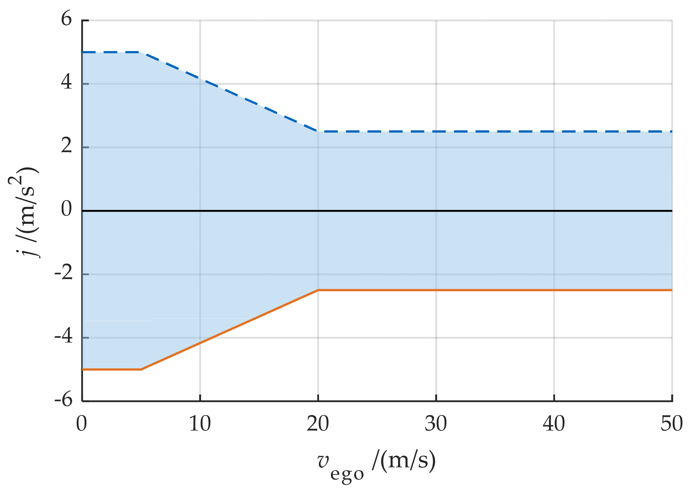
| m/s2 | 1 | 2 | 4 | Maximum acceleration of ACC | |
| m/s3 | 2 | 5 | 10 | Maximum jerk of ACC | |
| km/h | 5 | 20 | 40 | Tolerance speed for overtaking |
| Valid. RMSE | Comfort | Safety | Swiftness | Economy |
|---|---|---|---|---|
| 256 points | 0.506 | 0.185 | 0.234 | 0.079 |
| 512 points | 0.424 | 0.157 | 0.191 | 0.082 |
| 1024 points | 0.363 | 0.141 | 0.157 | 0.075 |
| 2048 points | 0.354 | 0.123 | 0.141 | 0.068 |
| Comfort | Safety | Swiftness | |
|---|---|---|---|
| Model RMSE | 0.363 | 0.141 | 0.157 |
| Parameter set RMSE | 0.440 | 0.239 | 0.255 |
| Parameter | Unit | Ref. Value | Comfortable | Safe | Swift |
|---|---|---|---|---|---|
| s | 2 | 2.43 | 2.40 | 0.65 | |
| - | 0.7 | 0.50 | 1.43 | 1.49 | |
| - | 1 | 1.00 | 1.30 | 0.86 | |
| - | 0.07 | 0.15 | 0.04 | 0.12 | |
| - | 1 | 0.80 | 0.80 | 1.06 | |
| m/s2 | 2 | 1.93 | 1.46 | 3.91 | |
| m/s3 | 5 | 5.96 | 4.52 | 8.61 | |
| km/h | 20 | 26.00 | 20.77 | 11.16 |
Publisher’s Note: MDPI stays neutral with regard to jurisdictional claims in published maps and institutional affiliations. |
© 2022 by the authors. Licensee MDPI, Basel, Switzerland. This article is an open access article distributed under the terms and conditions of the Creative Commons Attribution (CC BY) license (https://creativecommons.org/licenses/by/4.0/).
Share and Cite
Duan, X.; Schockenhoff, F.; Koch, A. Implementation of Driving Cycles Based on Driving Style Characteristics of Autonomous Vehicles. World Electr. Veh. J. 2022, 13, 108. https://doi.org/10.3390/wevj13060108
Duan X, Schockenhoff F, Koch A. Implementation of Driving Cycles Based on Driving Style Characteristics of Autonomous Vehicles. World Electric Vehicle Journal. 2022; 13(6):108. https://doi.org/10.3390/wevj13060108
Chicago/Turabian StyleDuan, Xucheng, Ferdinand Schockenhoff, and Alexander Koch. 2022. "Implementation of Driving Cycles Based on Driving Style Characteristics of Autonomous Vehicles" World Electric Vehicle Journal 13, no. 6: 108. https://doi.org/10.3390/wevj13060108
APA StyleDuan, X., Schockenhoff, F., & Koch, A. (2022). Implementation of Driving Cycles Based on Driving Style Characteristics of Autonomous Vehicles. World Electric Vehicle Journal, 13(6), 108. https://doi.org/10.3390/wevj13060108