Article

Modeling and Simulation of Traction Power Supply System for High-Speed Maglev Train

College of Electrical Engineering, Zhejiang University, Hangzhou 310027, China
*
Author to whom correspondence should be addressed.
World Electr. Veh. J. 2022, 13(5), 82; https://doi.org/10.3390/wevj13050082
Submission received: 16 March 2022 / Revised: 30 April 2022 / Accepted: 6 May 2022 / Published: 9 May 2022

Abstract

:
The electromagnetic suspension high-speed maglev train system uses long-stator linear synchronous motors (LLSMs) as levitation and traction mechanisms. In this paper, the modeling and simulation of the traction power supply system for the maglev train are performed. The simulation models include transformers, converters, variable-length cables and LLSMs of both two sides and two ends; meanwhile, the corresponding control and segmented power supply strategies, including the two-step method and three-step method, are implemented. Based on the system model, the operational performance of the high-speed maglev power supply control system is verified, and the fault performances under open circuit and short circuit are also analyzed. The whole simulation modeling and results have important reference significance for the research of high-speed maglev technology.

1. Introduction

Maglev technology is contactless in application; there is no wear and friction, thus increasing the efficiency and service life of the system. These characteristics make it applicable in many fields, such as maglev planar motors [1], magnetic bearings [2], maglev sliders [3], and maglev trains. As a land transportation vehicle, a maglev train can travel without contacting with the track and has many advantages in terms of travel speed and safety performance; thus, it has broad development prospects [4]. Because of the high manufacturing and testing costs of the maglev train system, the reliability and correctness of the system need to be verified by simulation before prototype production.
The whole system of the maglev train consists of many subsystem; thus, the research is divided into several aspects. Research on the maglev train has mainly focused on magnetic levitation, guidance, propulsion and power supply [5].
In terms of levitation techniques, two methods are generally used, i.e., electromagnetic suspension (EMS) and electrodynamic suspension (EDS). They are distinguished by the type of levitation force, which is attraction and repulsion, respectively. To ensure the safety of the maglev train, the airgap must be maintained under different circumstances. The neural network-based supervisor controller is designed to guarantee the vertical security of the EMS system [6]. There are also studies exploring the superiority of the high-temperature superconducting implemented in the EDS system [7,8].
Guidance systems are utilized to provide guiding forces against lateral displacement in situations such as bends or strong crosswinds. In particular, the design of guide magnet and robust control method have been studied [9,10].
Maglev trains generate propulsion force by linear motors, which mainly include linear induction motors (LIMs) and linear synchronous motors (LSMs). In high-speed maglev train applications, LSMs are more suitable due to their higher efficiency and power factors. The circuit characteristics and magnetic characteristics of the LSM implemented in the maglev train are analyzed using the analytical method or the finite element method [11,12]. Based on the motor model, the corresponding traction system can be built, and the operation of the whole train system under different working circumstances can be tested [13]. In order to cope with unknown situations such as changes in motor parameters or external disturbances, different kinds of fuzzy control are used to improve the robustness of the train control [14,15]. To give a more realistic control of the designed models, it is also an option to use the interconnectivity between software to realize the connection of the designed motor and control system [16].
The power supply of the whole system is classified into track power supply and vehicle power supply. Due to the long stator model of maglev trains, the segmented power supply to the stator on the track is required [17]. In addition, the vehicles need power supply from the ground side to feed the levitation, propulsion, etc. At low speeds up to 100 km/h, the maglev train can be powered by mechanical contact, while at high speeds, mechanical contact is no longer applicable. The linear generator integrated into the vehicles can produce power from the traveling electromagnetic field as the train is moving forward [18]. As in the wireless power transmission in other contactless applications, wireless power charging systems are applied in the high-speed maglev train system to realize contactless power supply for the vehicles [19,20].
In this paper, the traction power supply system of the EMS high-speed maglev train was introduced. The main purpose of the paper is to achieve the travel speed of high-speed maglev trains up to 600 km/h through the designed traction power supply system and verify the effectiveness and correctness of the system logic and control algorithm through simulation. The focus of this paper is to comprehensively model the track power supply system and the corresponding LLSM, to apply and compare the effects of different segmented power supply strategies, and to study the impact of the power supply system on the grid under fault conditions.

2. Traction Power Supply Simulation Model

2.1. Converter Model

Through the substation’s step-down, rectification and inversion, the grid voltage is converted into the adjustable voltage needed for high-speed maglev trains. In linear motors, the speed is proportional to the fundamental frequency of the current, so in the application of high-speed maglev trains, the frequency of the fundamental current of the traction power supply system is high, which imposes higher demands on the converters in the substation. The overall structure of the converter in the substation is shown in Figure 1.
To achieve fewer switching losses and fewer harmonics, a three-level neutral point clamped (NPC) power converter is implemented. There are two converters in one set of converters. When the train is at low speed, two converters are directly connected in parallel to obtain a higher drive current, so that the train can obtain greater thrust and acceleration. Since the counter-electromotive of the train increases with the speed, higher voltage is required when the train is at high speed. There are two ways in the model to increase the voltage level. The first connects two converters in series through transformers, and if a further voltage boost is required, it is achieved by changing the voltage ratio of the transformer bank at the back end, as shown in Figure 1.

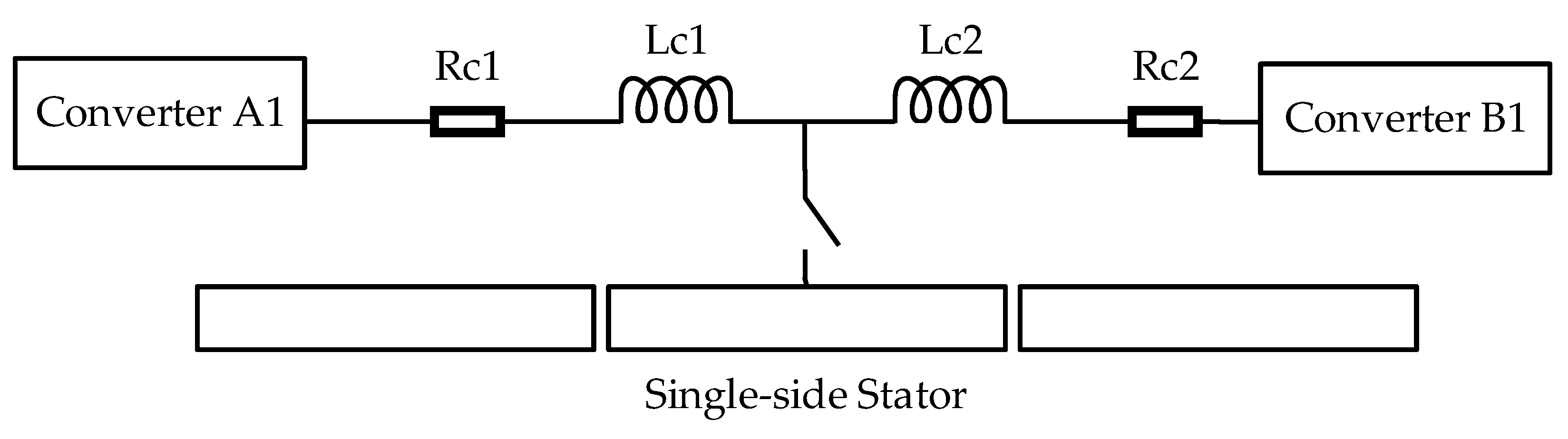
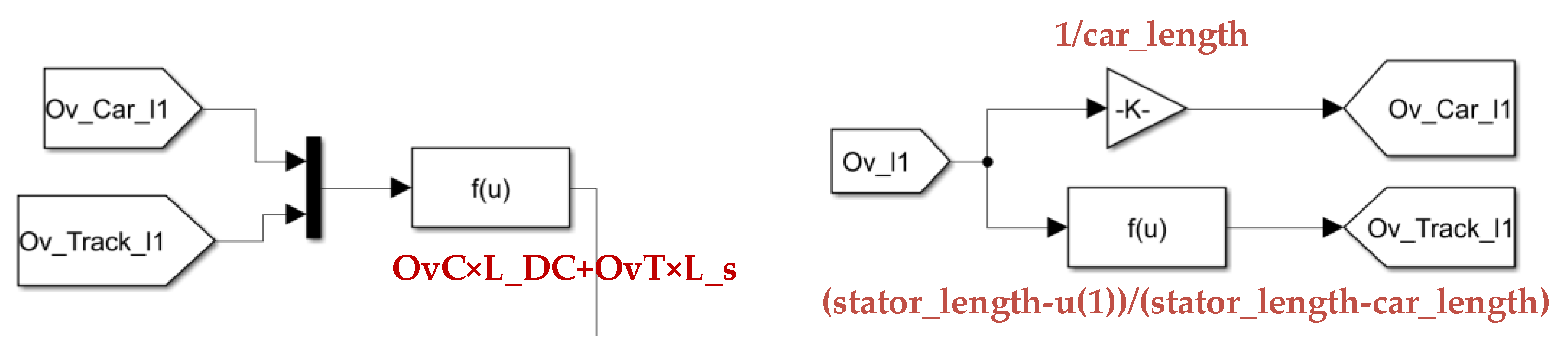
2.2. Variable-Length Cable Model

In order to provide sufficient output power, the system uses a double-ended power supply mode. Two sets of converters at each end of the power supply cable are connected in parallel to supply the train stator. The entire cable is powered as shown in Figure 2.
The voltage drop on the impedance of the cable needs to be compensated to overcome the circulating current caused by the parallel connection. The distance from the train to the substation at both ends changes from time to time during operation, resulting in the variation of the impedance of the cable before and behind the train. It is necessary to calculate the impedance of the cable to be compensated according to the distance the train travels and then adjust the output power of the converters. The impedance of the cable is calculated by multiplying the distance from the train to the substation by the impedance in units.

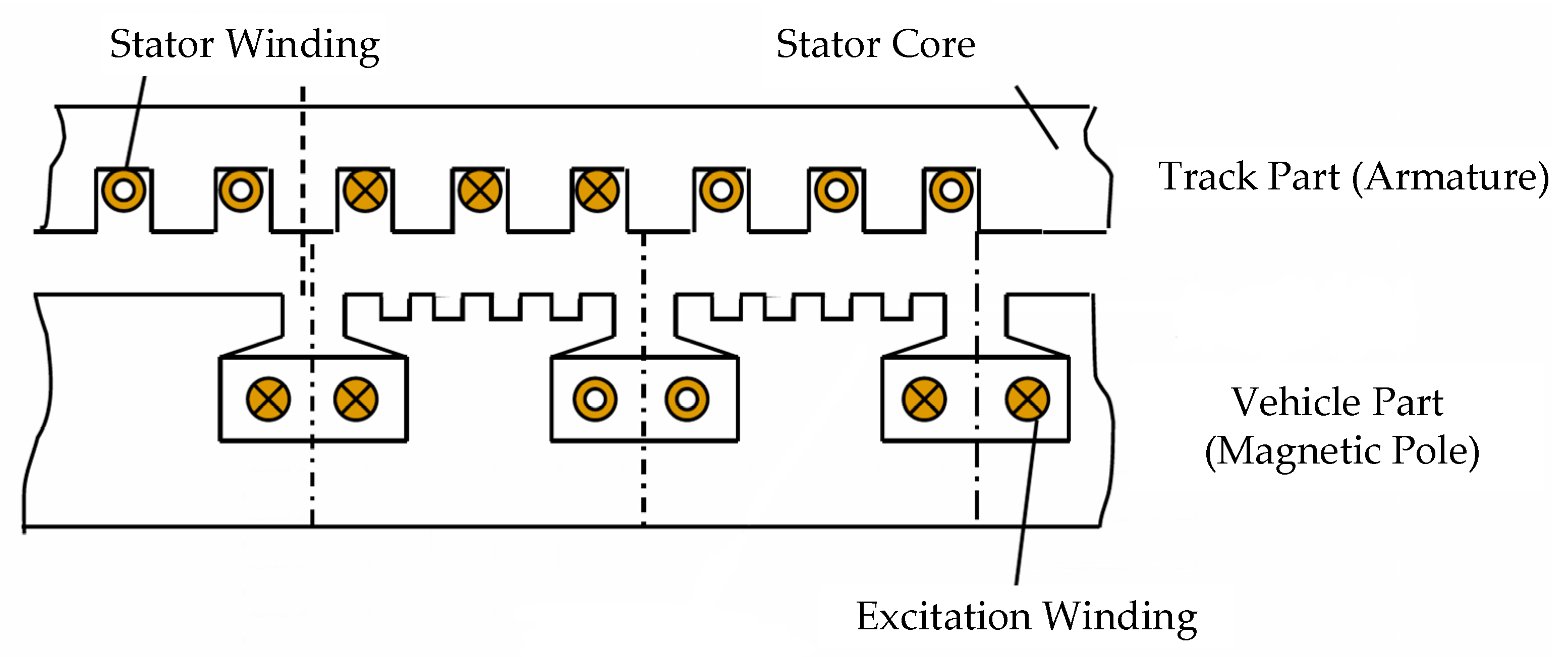
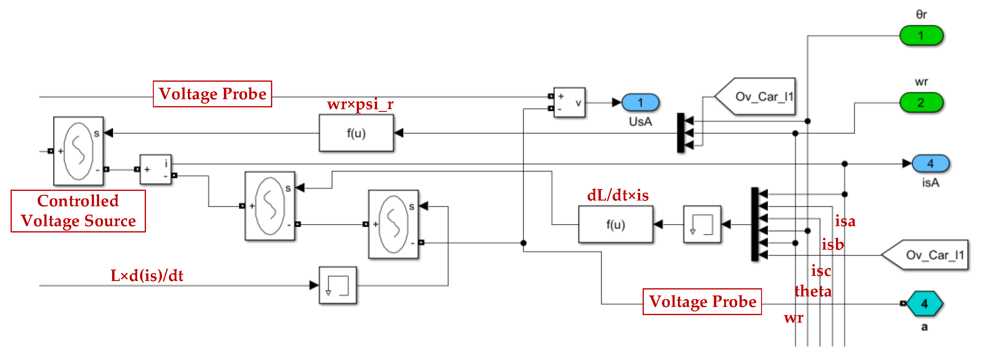
2.3. Long Stator Linear Synchronous Motor (LLSM) Model

2.3.1. Introduction of Motor Model

In this paper, electrically excited LLSM models, which have a high efficiency and power factor, are used in the maglev train system. The motor lateral profile is shown in Figure 3.
The long stators of the LLSM are mounted on the track with a segmented stator core. The excitation magnet (magnetic pole) is mounted underneath the vehicle, and the excitation winding is wound on the excitation core, which is fed with DC current to generate the magnetic field. Four slots on the surface of the main pole shoe are used to place the linear generator windings, which are used to generate power to the vehicle. The motor has windings in both the stator and the mover, which require a large number of conductors due to the long distance of the track. In order to save cost and to make the motor lighter, aluminum is used as a conductor in this maglev train system. As mentioned above, the converters need to provide a high voltage to the motor to overcome the large counter-electromotive generated by the motor at high speed. In this motor, the number of conductor turns in each slot is one, and the stator is segmented every 1200 m, so the voltage of the motor is less than 10 kV. At this voltage level, the insulation requirements can be met by using cable type windings in the motor.
Both suspension force and traction force are generated by the LLSM; in order to minimize the coupling of suspension force and traction force, the control method of i d = 0 is used. In this way, the magnetic field in the airgap is completely determined by the excitation current, and the traction force can be adjusted by changing the armature current, thus maximizing the decoupling of the suspension force and traction force. In this paper, the part of the vehicle is simplified into the constant magnetic poles, since the i d = 0 control method is applied.
The motor models are based on equations of the circuits and motion in a three-phase coordinate system and are built using discrete electrical components, thus increasing flexibility. The length of the single stator on the track is 1200 m, while the total length of the train is 120 m, so the overlapping and non-overlapping parts between the movers in the train and the stators on the track needs to be considered comprehensively in the modeling process. At the same time, in order to reduce the thrust fluctuation when switching between stator sections, the stators on the left and right sides of the trains are installed at a distance of 600 m in a staggered manner, thus staggering the position of segmented power supply. Therefore, in order to simulate the train more realistically, four motors need to be modeled simultaneously. The modeling of the four motors, named L1, L2, R1, and R2, is shown in Figure 4. Since the train length is much smaller than the stator length, the mover in the train overlaps up to three stator segments at the same time, so the periodic arrangement of the four motors is sufficient for describing the driving state of the train.

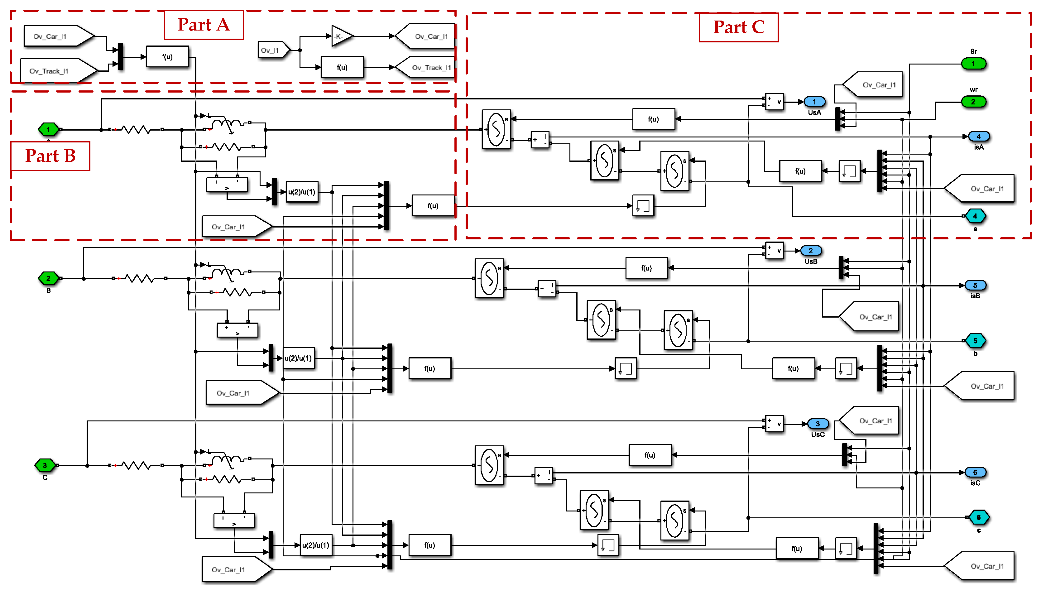
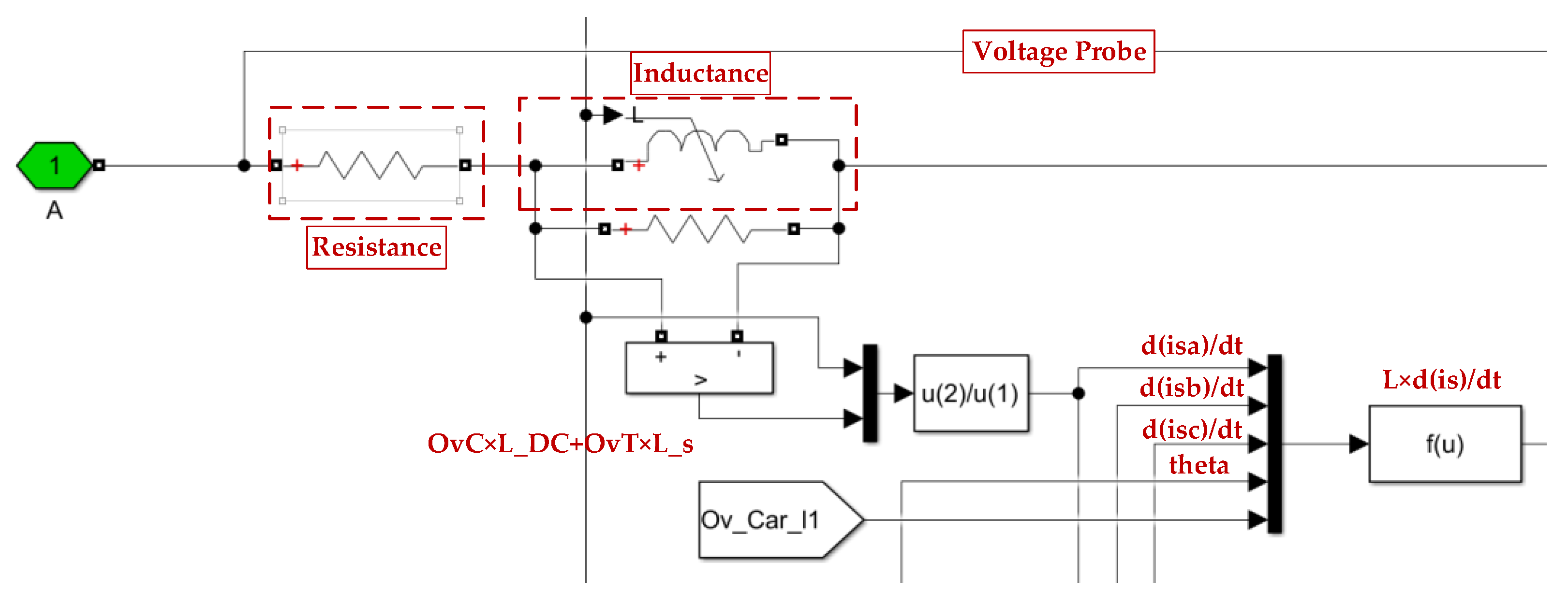
2.3.2. Motor Modeling Method

In the three-phase coordinate system, the voltage and flux linkage equations for a symmetrical motor can be expressed as
u s a u s b u s c = R s i s a i s b i s c + p ψ s a ψ s b ψ s c ψ s a ψ s b ψ s c = L a a M b a M c a M a b L b b M c b M a c M b c L c c i s a i s b i s c + ψ r c o s θ c o s θ 2 3 π c o s θ + 2 3 π
where u s A B C and i s A B C represent the three-phase components of stator voltage and stator current, respectively, R s is the stator resistance, p is the differential operator, ψ s A B C represents the three-phase components of the stator flux linkage, L i i i = a ~ c is the self-inductance of three-phase windings, M i j i j , i = a ~ c , j = a ~ c is the mutual inductance of three-phase windings, ψ r is the coupling part of the excitation flux linkage to the stator as mentioned above, and θ is the electrical angle. In the symmetrical motor, the self and mutual inductance of the three phases are equal and can be expressed as
L a a = L s σ + L D C + L A C c o s 2 θ L b b = L s σ + L D C + L A C c o s 2 θ 2 π 3 L c c = L s σ + L D C + L A C c o s 2 θ + 2 π 3
M a b = M b a = M D C + M A C c o s 2 θ + 2 π 3 M b c = M c b = M D C + M A C c o s 2 θ M a c = M c a = M D C + M A C c o s 2 θ 2 π 3
where L s σ is the leakage inductance, L D C and M D C are the DC components of self and mutual inductance, and L A C and M A C are the AC components of self and mutual inductance, whose frequency is twice the electrical frequency. In the non-salient pole motor, the AC components of self and mutual inductance are zero. Combining the above analysis, the derived voltage and current equations can be expanded as follows:
u s a u s b u s c = 2 L A C s i n 2 θ M A C s i n 2 θ 2 π 3 M A C s i n 2 θ + 2 π 3 M A C s i n 2 θ 2 π 3 L A C s i n 2 θ M A C s i n 2 θ M A C s i n 2 θ + 2 π 3 M A C s i n 2 θ L A C s i n 2 θ i s a i s b i s c + L a a M b a M c a M a b L b b M c b M a c M b c L c c p i s a i s b i s c + R s i s a i s b i s c ω r ψ r s i n θ s i n θ 2 3 π s i n θ + 2 3 π
where ω r is the electrical angular velocity. Since the modeling needs to consider the overlapping and non-overlapping of the stator and mover, the inductance needs to be related to the length of the overlapping part in a way that will be described in the following. Taking L1 as an example, the modeling method based on the voltage and flux linkage equations is shown in Figure 5.
In order to illustrate more clearly how the motor is modeled internally, the circuit model of phase A within the motor is divided into three parts, as is shown in Figure 5 and will be explained in detail, and the circuit models of phase B and C are based on the same principles as phase A.
Part A of model of is shown in Figure 6, and the equations in each box have been labeled near the box. “Ov_l1” represents the overlapping part of the stator and mover of the motor L1, which is calculated by the position of the vehicle on the whole track. After further calculation, the overlapping and non-overlapping parts of the stator and the mover in motor L1 can be obtained, which are represented by “Ov_car_l1” and “Ov_Track_l1” in the figure, respectively. For convenience, “Ov_car_l1” is denoted by “OvC”, and “Ov_track_l1” is denoted by “OvT”. In the following modeling and calculation, the self and mutual inductance of the motor need to be multiplied by “OvC”, and the leakage inductance of the motor needs to be multiplied by “OvT”, so as to realize the simulation of the overlapping and non-overlapping parts of the motor.
Parts B and C of the model are shown in Figure 7 and Figure 8, respectively. In Part B, the resistance and inductance are connected in series. The resistance is the stator resistance. The voltage drop on the resistance is the third part of the voltage of phase A in Equation (4). The inductance uses the value passed from Part A, i.e., “OvC × L_DC + OvT × L_s”. By dividing the voltage drop on the inductance with the value of the inductance, the derivative of the current is obtained, that is, p i s a . We multiplied the inductance and the derivative of the current, then added the voltage drop on the inductance, to obtain the second part of the voltage of phase A in Equation (4). It is represented as “L × d(is)/dt”, and its specific expression is L s σ × p i s a × O v T + ( ( L a a L s σ ) × p i s a + M b a × p i s a + M c a × p i s c ) × O v C . In Part C, “dL/dt × is” represents the product of the current and the derivative of the inductance. In this way, the first part of the voltage of phase A in Equation (4) is obtained, and its expression is 2 × L A C s i n 2 θ × i s a + M A C s i n 2 θ 2 π 3 × i s b + M A C s i n 2 θ + 2 π 3 × i s c × O v C . “wr × psi_r” is the fourth part of the voltage of phase A in Equation (4), and its expression is ω r ψ r s i n θ × O v C . By connecting the four parts in series with the controlled voltage source, the four parts can be added together, and the complete modeling of the voltage of phase A is achieved. The voltage probe, voltage measurement module and current measurement module are used to detect the voltage and current value of the motor, which are used for motor control.
After building the circuit model, the train’s motion model is built. The equation of the motion of the train is expressed as
x = 0 t v d t M d v d t = F x F z F x = L 1 , L 2 , R 1 , R 2 π τ Ψ d i q Ψ q i d
where x is the travel of the train, v is the running speed of the train, M is the total mass of the train, F x is the total traction force of the four linear motors, F z is the drag force during the train travel, which is positively related to the speed, τ is pole pitch of the motor, i d and i q are the components of the stator current on the d q coordinate system, and Ψ d and Ψ q are the components of the stator flux linkage on the d q coordinate system, calculated by the following formula:
Ψ d = L d i d + Ψ r Ψ q = L q i q

3. Traction Power Supply System Control Strategy

3.1. Single Motor Control Strategy

For three-level NPC power converters, a three-level space vector pulse width modulation method is used to generate a reference voltage based pulse signal. Each motor is controlled with a speed-current closed loop and i d = 0 control method.
Current control is mainly based on the current output from the converters after series or parallel connection. The feedback value detection point of the current loop is set at the switching station. It means that the feedback value of the current needs to be corrected for the primary and secondary ratios when the train is running at high speed and the voltage is increased through the transformers. At the same time, when two sets of converters in a substation are connected in series or parallel, the output rated current values are different. In the parallel state, when the output rated current value of a single converter is i A, the parallel output is 2 i A. While in the series state, considering the capacity of the converter, the output rated current of a single converter cannot be directly set to 2 i A but needs to be reduced and set to 1.6 i A in this system. So the feedback value of the current when switching from parallel to series also needs to be corrected.
The deviation of the speed loop generates the initial q-axis given current i q 0 * by the PI regulator. Since the cable is supplied with a double-ended power supply, the voltage drop on the impedance on the cable needs to be compensated in order to ensure that both substations have the same potential for the same output power. The distance travelled by the train as a proportion of the total distance travelled is denoted as x 0 , and the remaining distance is 1 x 0 . In order to keep the voltage drop on the impedance between the train and the substations at the two ends the same, the initial q-axis given current is multiplied by a factor of 1 x 0 and x 0 for the starting and ending stations, respectively. The product with 1 x 0 and x 0 will reduce the current given value and cannot reach the rating. In order to maximize the total output power of both substations at the same time, it is necessary to amplify the given current to raise the output power. Thus, the given current for the two substations is multiplied by a factor m , which is defined as
m = s u p 1 1 x 0 , 1 x 0
In this way, the given current of the two substations and the current supplied to the motor can be expressed as
i q 1 * = m 1 x i q 0 * i q 2 * = m x i q 0 * i q * = i q 1 * k + i q 2 * k = m k i q 0 *
where i q 1 * and i q 2 * are the q-axis output current from the substations at both ends, i q * is the current delivered to the motor stator, k is the ratio of the rated current generated when the converter is switched from parallel to series or when the transformer changes voltage levels. In order to keep the given current of the motor from exceeding the rated current, it is necessary to give m a limiting value of k .

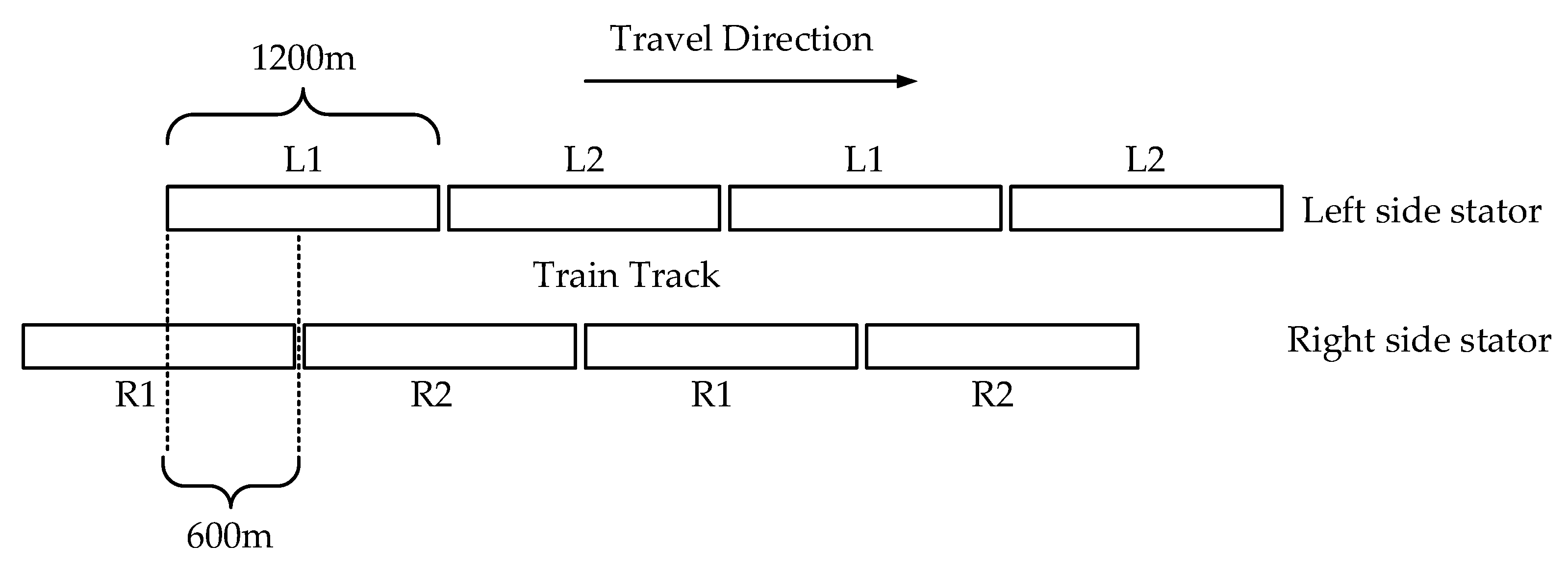
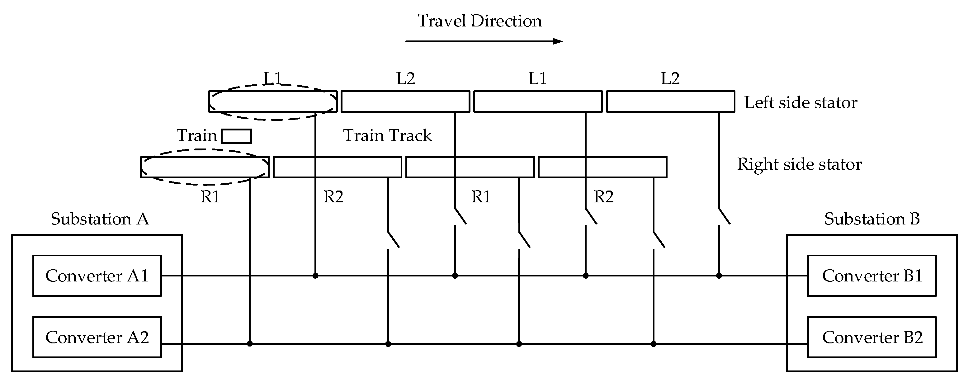
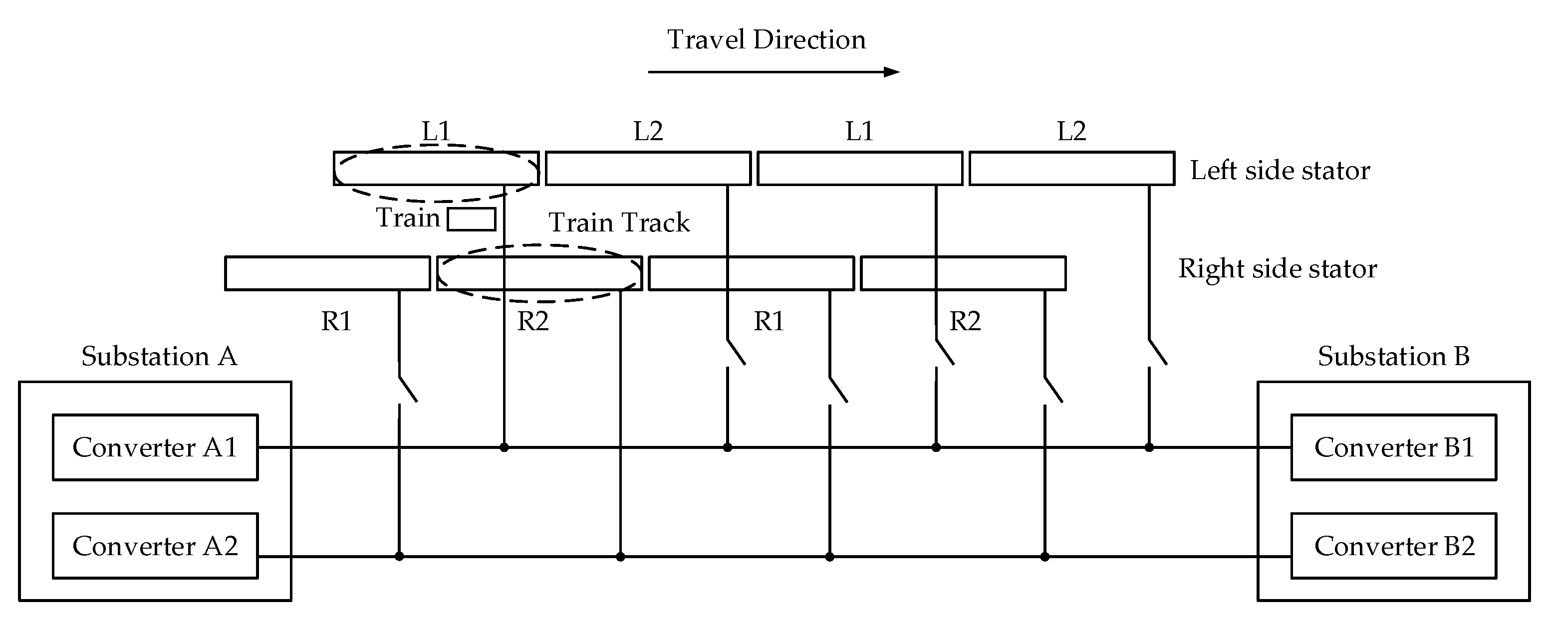
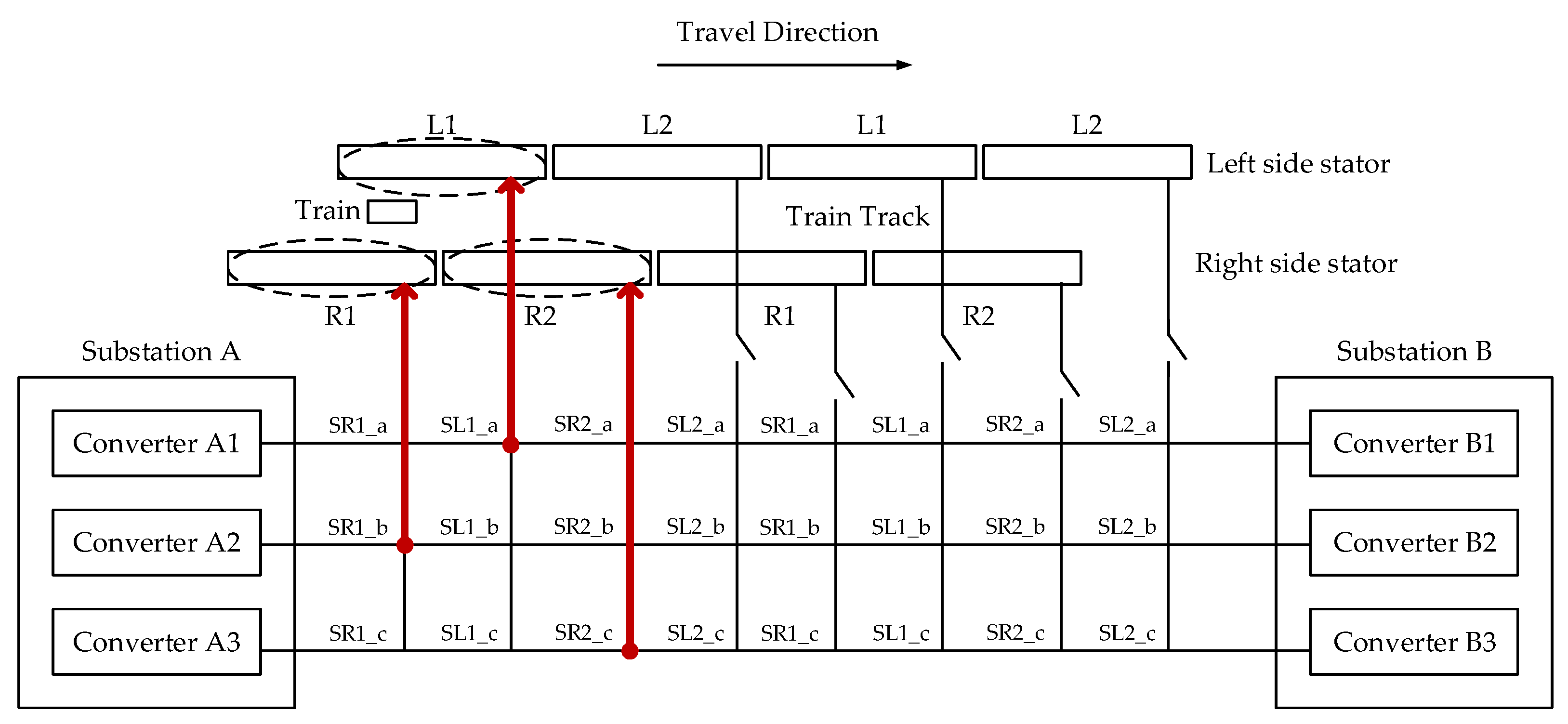
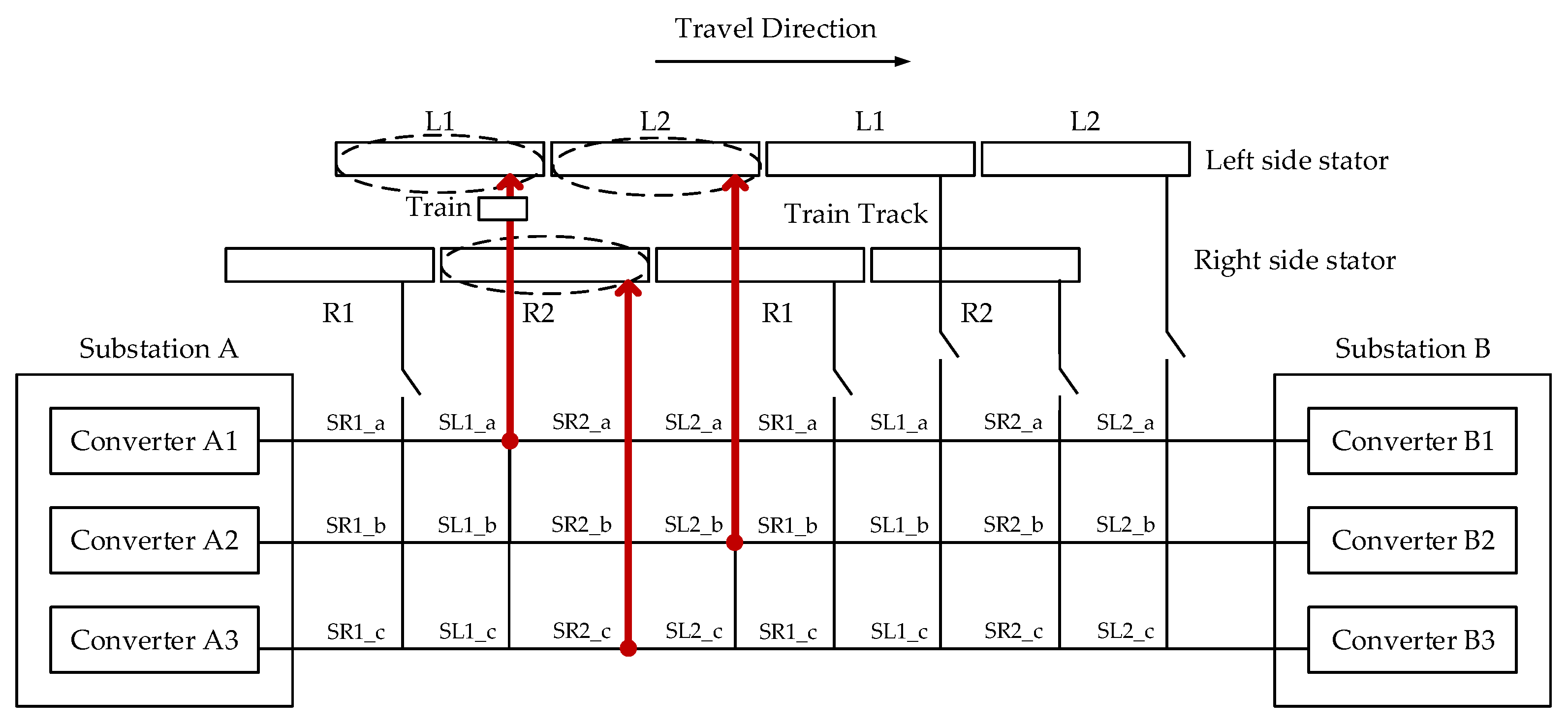
3.2. Stator Segmented Power Supply Method

Since the length of the stator is much longer than that of the mover, a stator segmentation power supply method is required, in which each stator on the track has a switching station that switches according to the position of the train.

3.2.1. Two-Step Method

In the two-step method, there are two sets of converters in the substation at each end of the cable. Two sets of converters on the same cable supply both stators on one side in a staggered manner, e.g., converter A1 and converter B1 supplying L1 or L2 together, converter A2 and converter B2 supplying R1 or R2. In the non-switching state, the method proposed in Section 3.1 is used to control the stator L1/L2 and R1/R2 at the left and right ends of the train, respectively, with two motors running together at each moment. In the switching state, the stator that the train is leaving is turned off, and its current is dropped to zero; then, the stator that the train is approaching is turned on. Since the switching positions of the two adjacent stators are staggered, thrust fluctuations occur during switching. The demonstration process of the two-step method is shown in Figure 9 and Figure 10, where the stator in the dashed box indicates it is powered.

3.2.2. Three-Step Method

In the three-step method, there are three sets of converters in the substation at each end of the cable, with a total of three sets of converters working together during the switching process. Each stator can be connected to different cables at different times via switching stations. The switching process of the three-step method is shown in Figure 11 and Figure 12. The switching station that connects the stator to the cable is indicated by the symbol SR1_a, etc. In the symbol SR1_a, for example, “R1” indicates the stator connected to this switching station and “a” indicates that the stator is connected to the first cable. The dashed box shows the stator being powered. The red line indicates the wire being powered, and the solid red dot indicates the connection point between the stator section and the three power supply cables. A combination of different switching states for the three sets of converters ensures that there is no drop in thrust when the train runs between different stators.
Based on the three-step method, when the train moves to the switching area, there are always two motors driving the train forward, so the train does not have the thrust fluctuation caused by stator segmentation. At the same time, no drop in thrust will allow the train to run at a faster speed and accelerate throughout its journey. In terms of equipment, compared to the two-step method, the converter equipment of the three-step method is increased by half, and the number of the switching stations is increased to three times that of the two-step method.

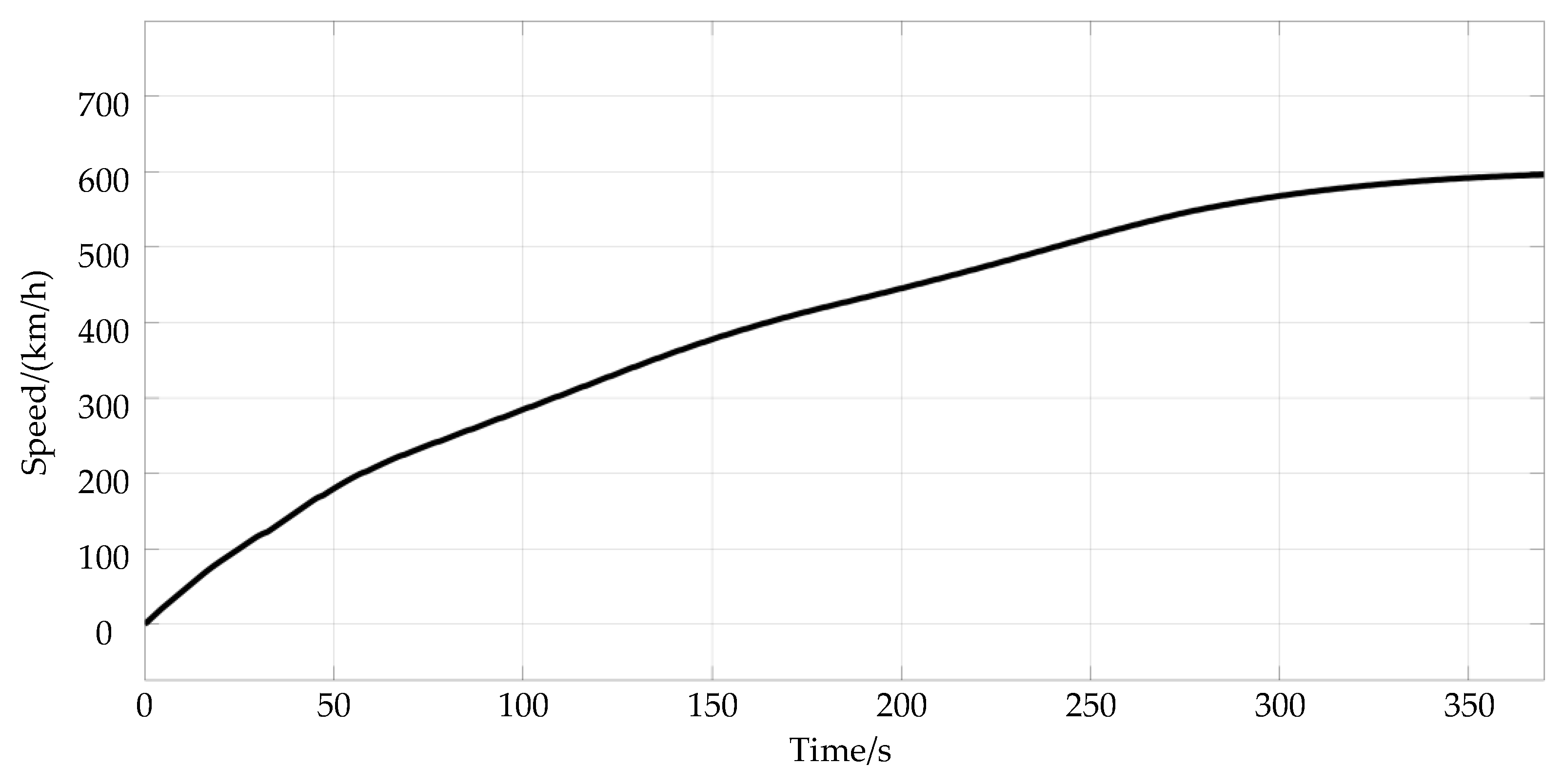
4. Models Simulation Results

In order to simulate and verify the motor models and control methods, the overall model of the high-speed maglev train platform is built and implemented in MATLAB/Simulink. The maximum driving speed of the train is set to 600 km/h, the simulation step is set to 10 μ s, and the parameters of the linear motor model are shown in Table 1. These parameters are from the TR08 high-speed maglev train. The self-inductance, mutual inductance, leakage inductance and mover flux linkage in Table 1 are all parameters when the motor’s stator and mover are fully overlapped. In the modeling, the overlap ratio between stator and mover is set to x o v e r l a p , then the self-inductance, mutual-inductance and mover flux linkage of a single motor are multiplied by x o v e r l a p , and the leakage-inductance is multiplied by 1 x o v e r l a p , so as to simulate the real driving situations of the train. Since the motor is the non-salient pole motor, the AC component of the inductance is zero, so the inductance value given in the table is the DC component of the inductance.
According to the parameters in Table 1, the train models using the two-step and three-step methods were tested, and the relevant results of the train simulation are described separately below.

4.1. Simulation Results of the Two-Step Method

When the two-step method is used, the speed simulation results of the train are shown in Figure 13. From Figure 13, it can be seen that the train reaches a speed of 600 km/h at 370 s, and the speed curve is smooth, which proves the effectiveness of the traction power supply system and control method.
The acceleration of the train is shown in Figure 14. The maximum acceleration is 1.4   m / s 2 , and the acceleration decreases with increasing speed. This is because, as the speed increases, there will be parallel to series switching inside the substation as well as the increase of the transformer voltage level, which makes the output current of the substation decrease. In addition, the resistance of the train is positively related to the speed. It can also be seen that the acceleration dips at regular intervals, which is clearly caused by the drop in current and thrust during the stator segmented power supply in the two-step method.
In order to better observe the effect of the voltage ratio on the stator current, the values of the q-axis stator current at different voltage levels are shown in Figure 15, where K indicates the back-end transformer voltage ratio. It can be seen that the overall trend of the output q-axis stator current decreases as the converter is switched from parallel to series and the voltage level of the back-end transformer increases, which is consistent with the analysis. It can also be seen that the current increases during certain periods of time because the resistance of the train increases with speed and the output current of the converter needs to increase as well.
In Figure 15, it can be seen that the q-axis current in the stator winding fluctuates greatly at certain moments. One of these parts is shown in greater detail in Figure 16. There is much fluctuation in the q-axis current, mainly because the converter is over-modulated. During the driving process, as the transformer is connected in series and the voltage ratio increases, the converter becomes over-modulated when the voltage limit is reached, making it impossible to maintain a constant q-axis current. In addition, the transformer used is a power frequency transformer, which cannot achieve ideal amplification of the pulse width modulation voltage output from the converter, further exacerbating the impact. If the converter is not set up for overmodulation, sudden changes in train thrust and acceleration would occur when the transformer is connected in series or when the ratio changes, which is not permitted in train operation. Therefore, the acceleration curves in Figure 14 do not change abruptly after setting the overmodulation of the converter.
The q-axis current variation of the stator segmentation switching process is shown in Figure 17. It shows that the two-step method has a large drop in current during the switching process, as there is a delay between the turn-on time of the next stator and the turn-off time of the current stator.
The current output from the converters at both ends is shown in Figure 18 and Figure 19. Since the voltage drop on the cable needs to be compensated, from the prospective of the whole process, the output current of the converter at the start point decreases as the train runs, while the output current of the converter at the end point increases.

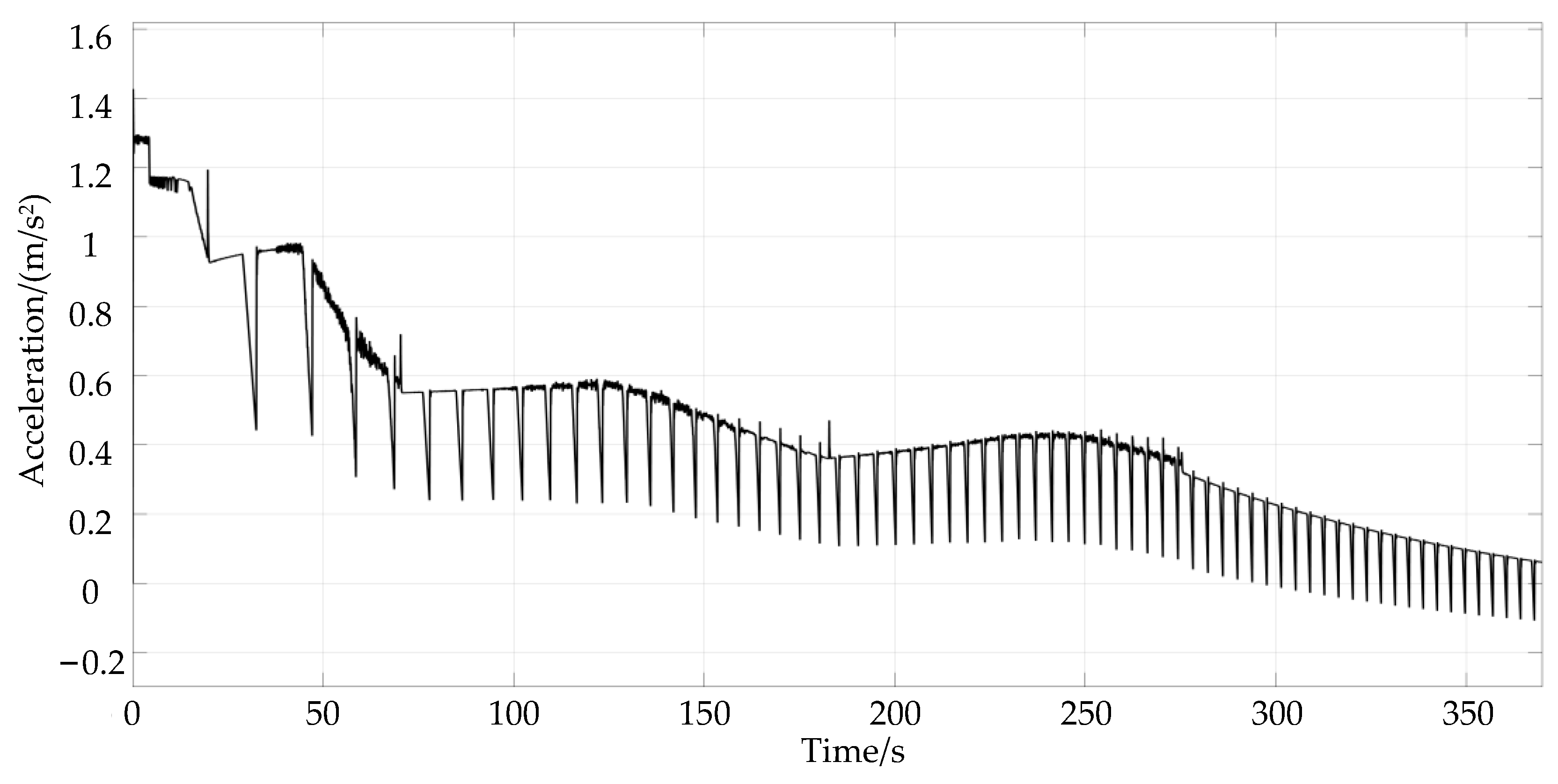
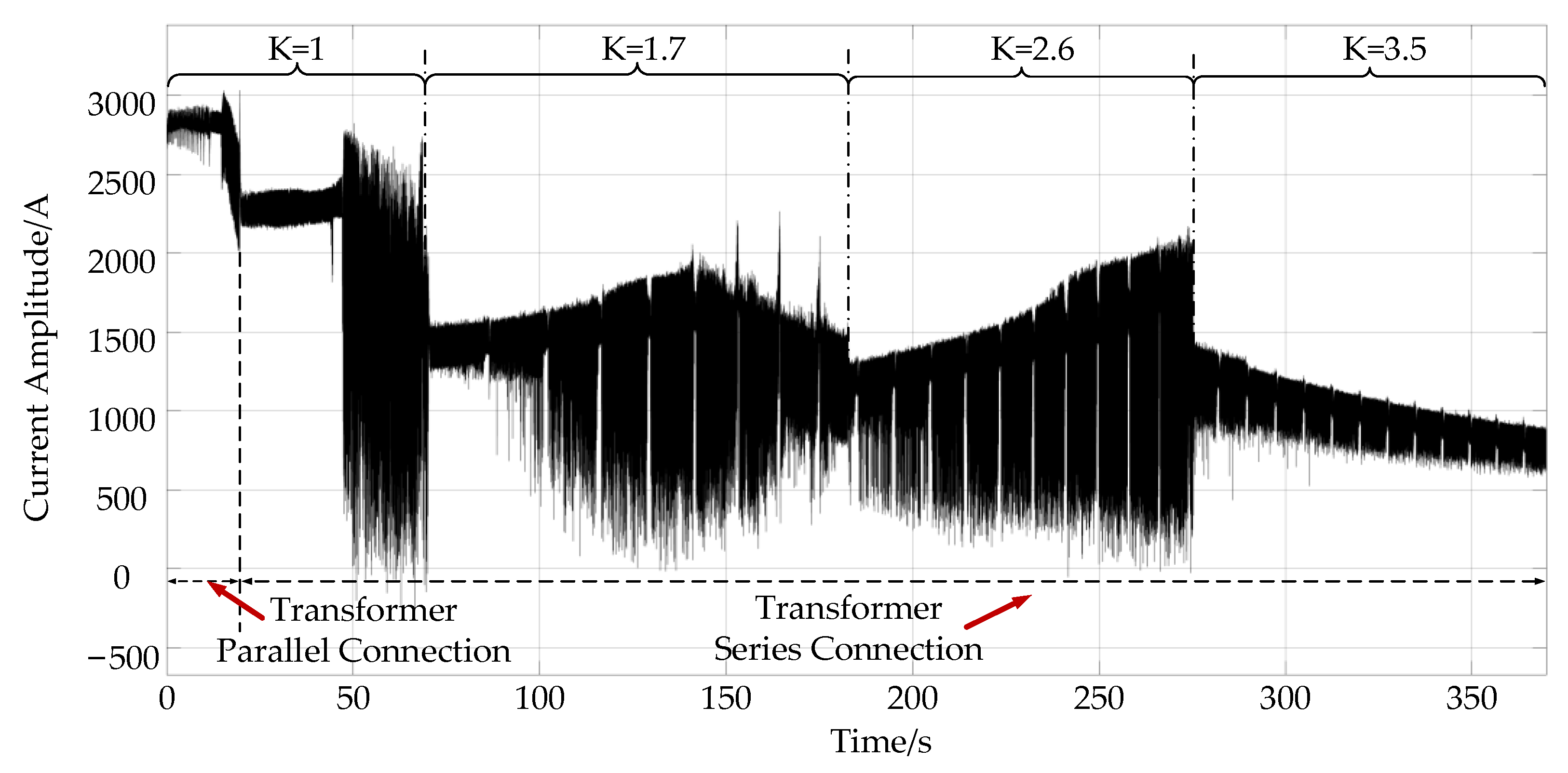
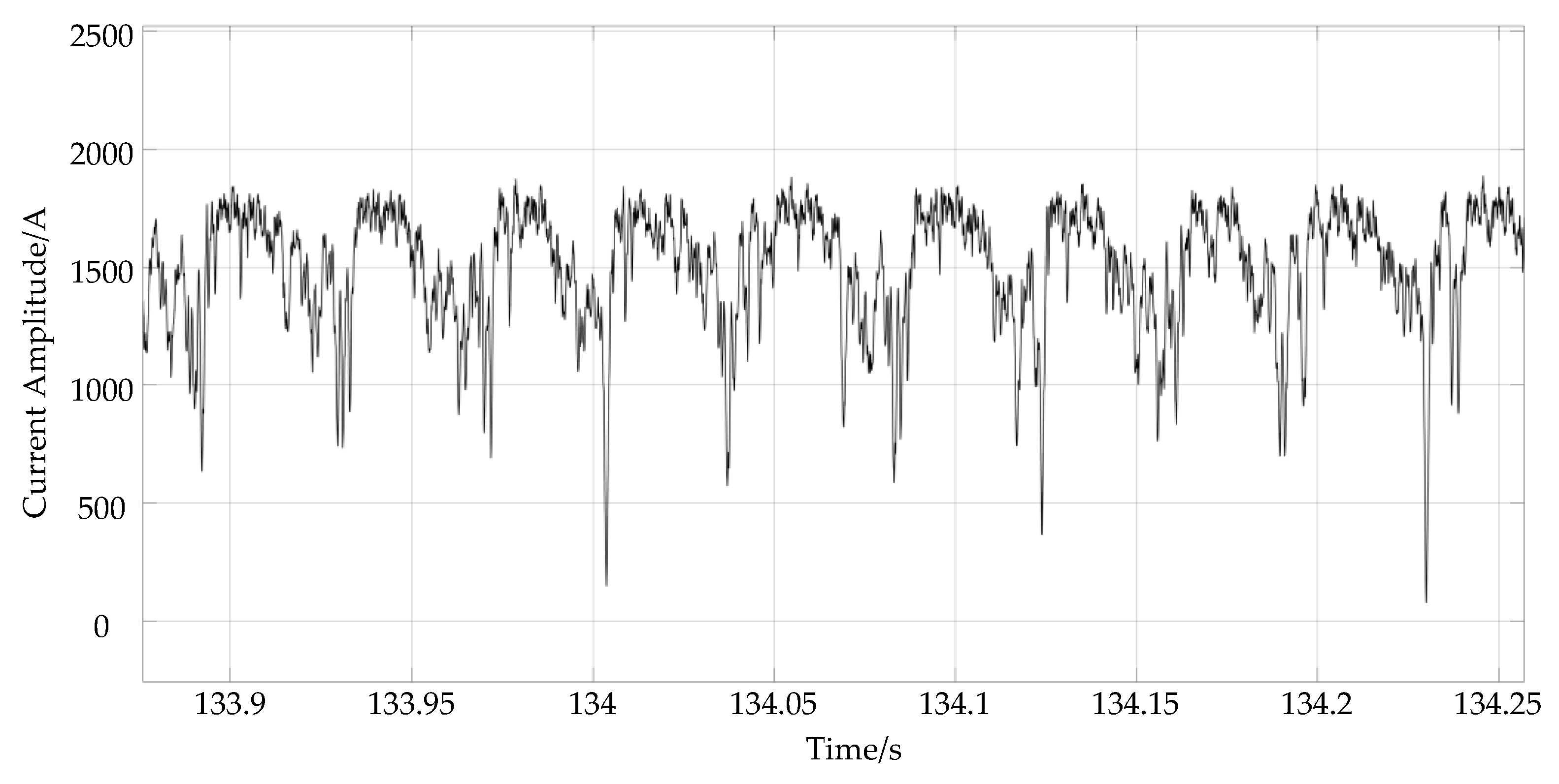
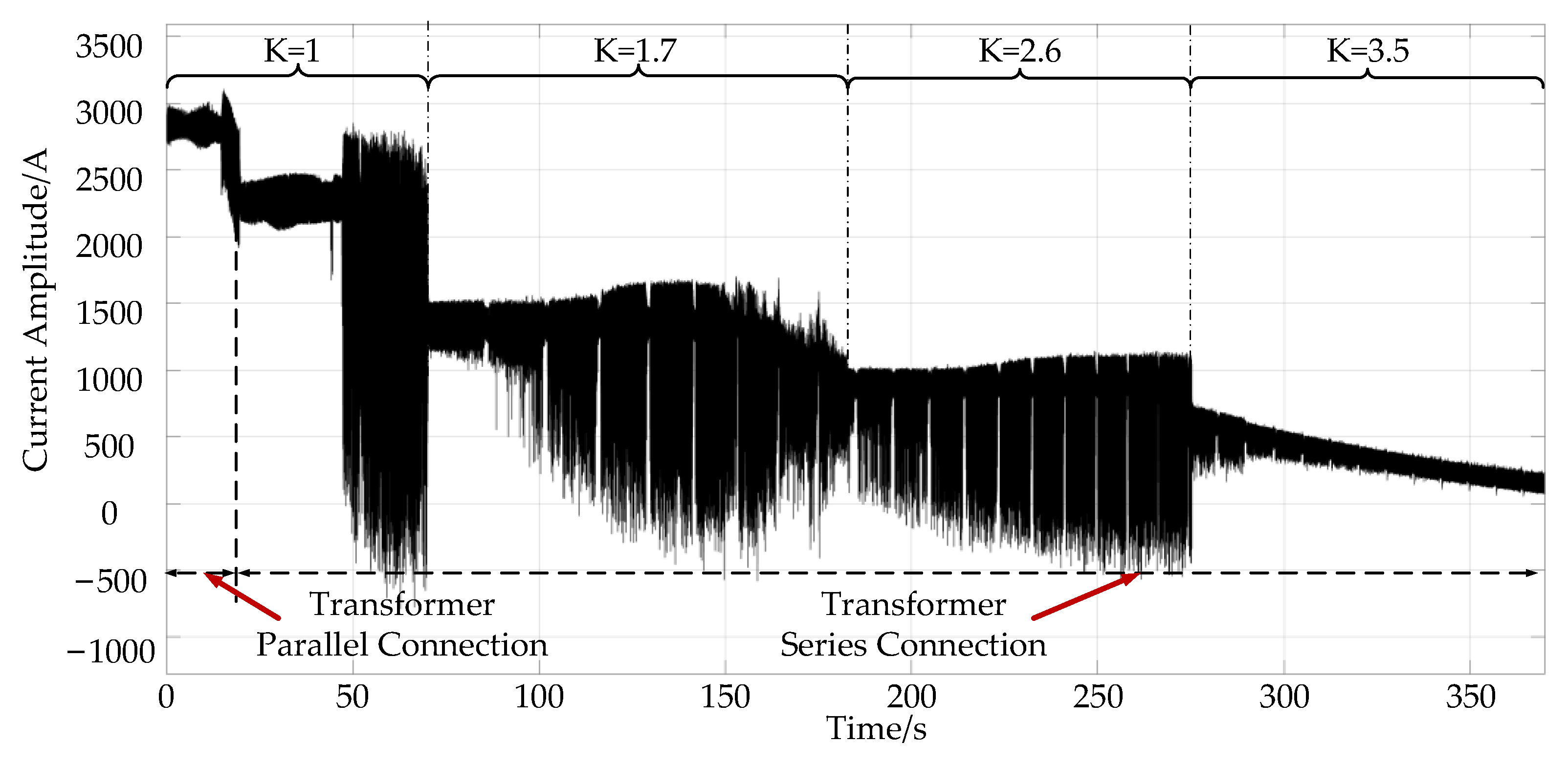
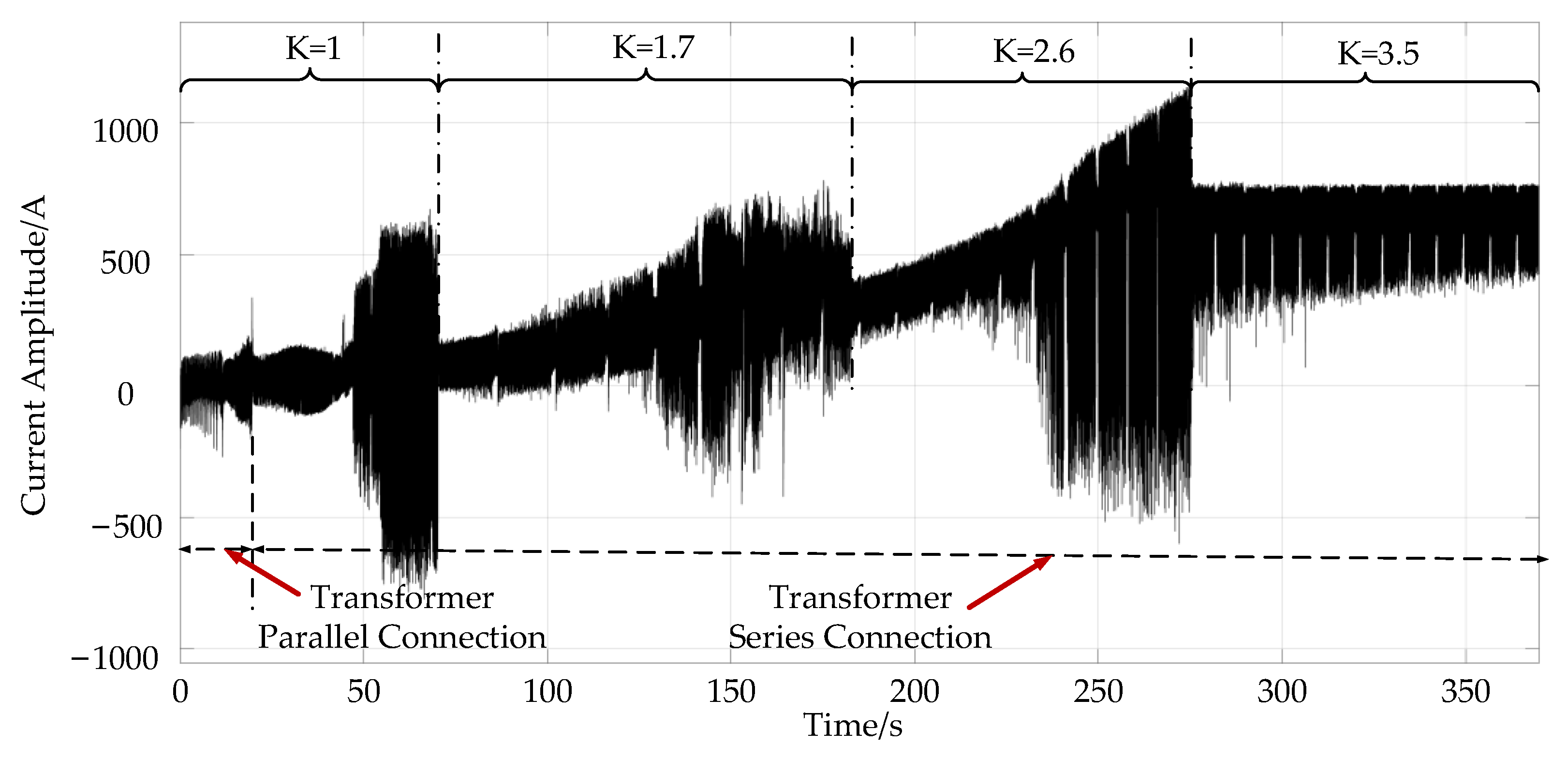
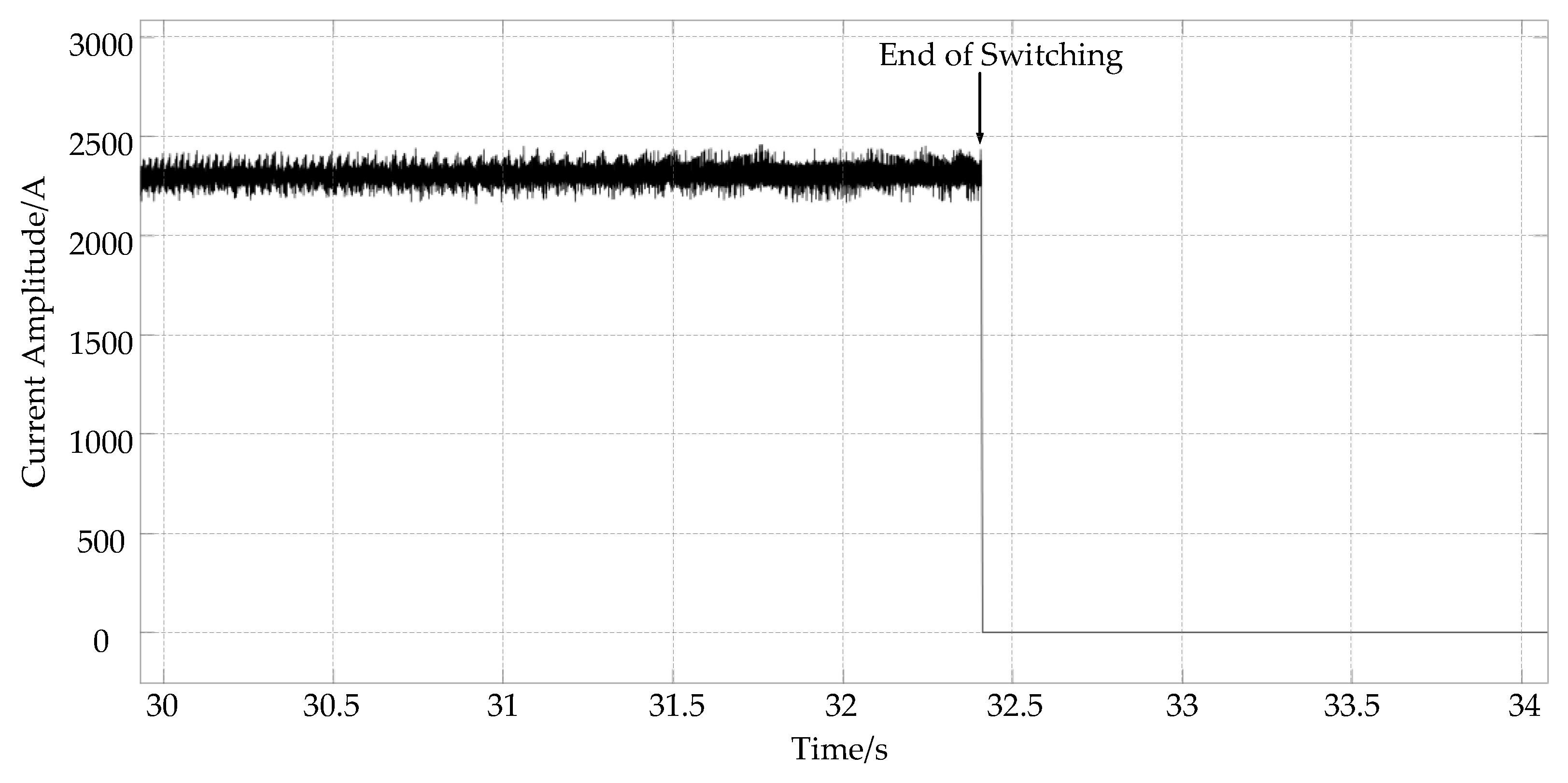
4.2. Simulation Results of the Three-Step Method

The main difference between the three-step method and the two-step method is that the stator segments are switched in different ways, so only the differences between the two methods are compared in the segmented power supply process. Figure 20 and Figure 21 show the q-axis current on the stator where the train is leaving (R1) and the stator where it is approaching (R2). It can be seen that stator R1 is disconnected at the end of the switching, and stator R2 remains powered throughout the switching process, thus showing that the q-axis current on the entire train does not drop in the two-step method.
The thrust of the train during the switching process is shown in Figure 22. It can be seen that during the switching process, since the stator current does not drop, the thrust does not drop either. Therefore, with other traction and power supply methods being the same, the acceleration of the train is greater during the whole driving process, making the train run faster and more stable when applying the three-step method.

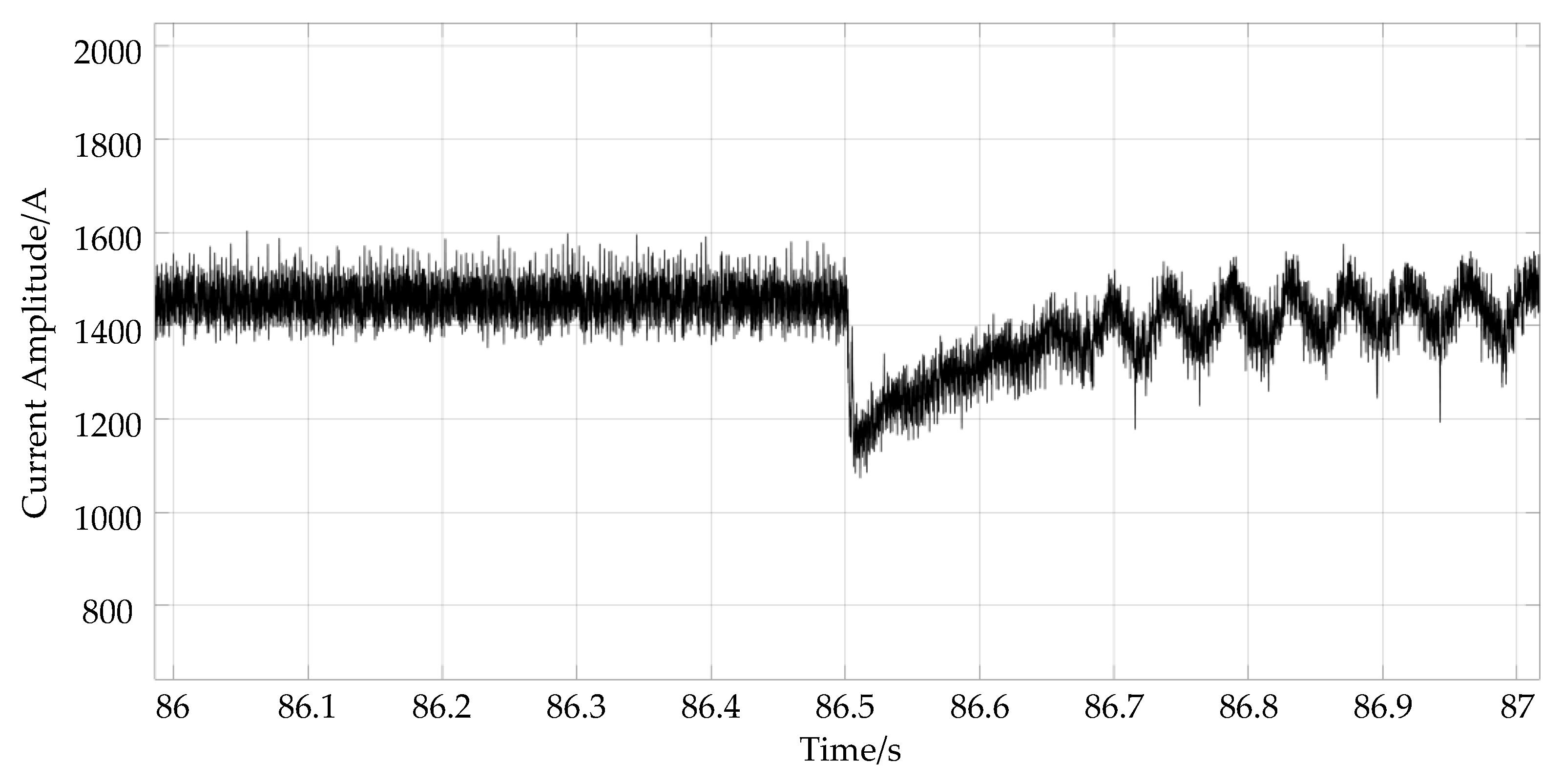
4.3. Simulation Results of LLSM with Faults

In the driving process of the motor, the faults of single-phase disconnection and phase-to-phase short circuit may occur; both failures may have impacts on the driving process of the train. Since the two-step and three-step methods have basically the same control strategy during non-switching, only the effects of faults in the two-step method are analyzed here. In the following simulations, the fault occurs at the tenth stator on the left side of the train.

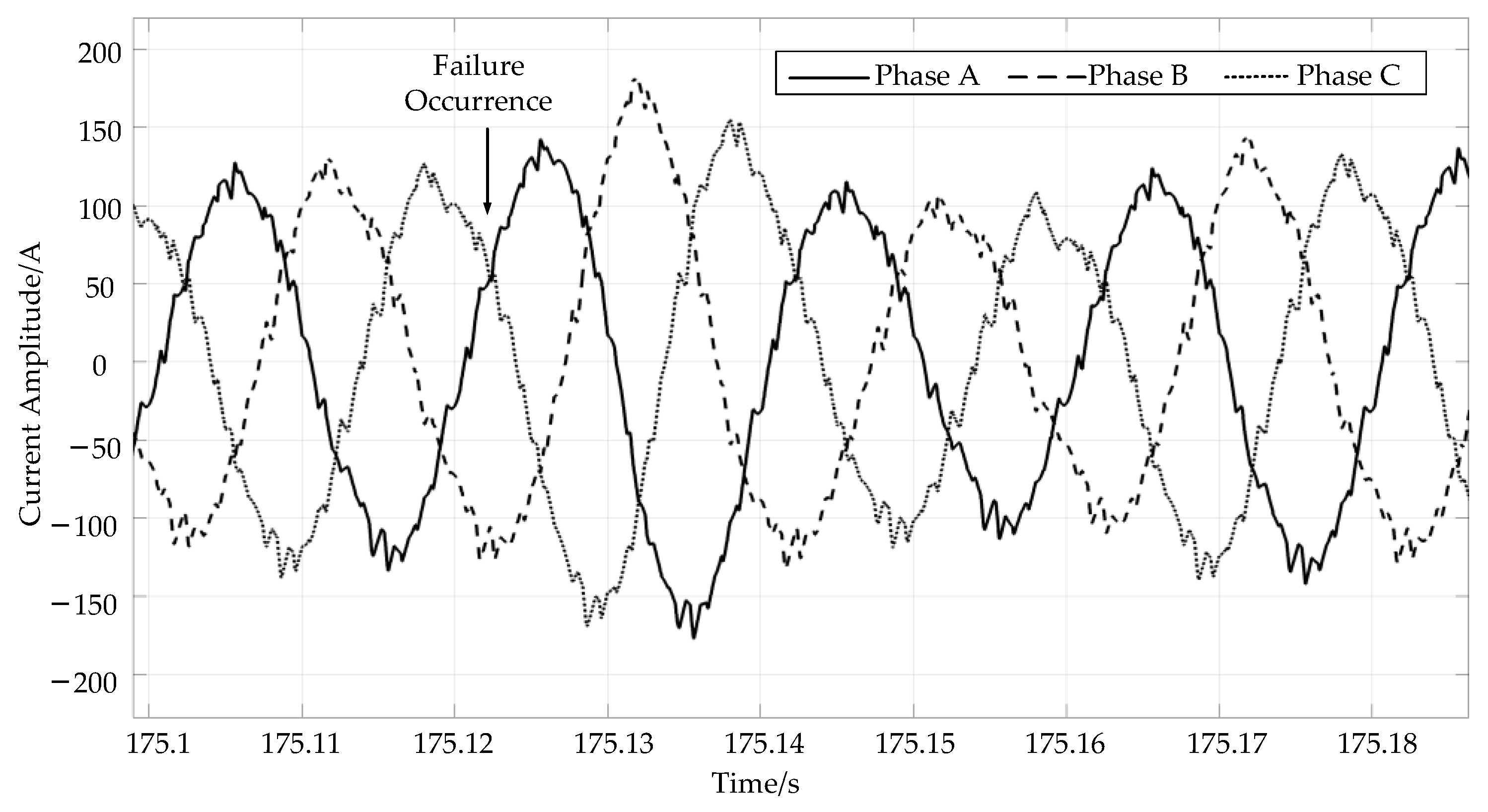
4.3.1. Single-Phase Disconnection Fault of LLSM

For a single-phase disconnection, the three-phase current on the stator is shown in Figure 23. It can be seen that when phase A is disconnected, the current of phase A becomes zero, and the current of the phase B and phase C have some distortion, which obviously affects the output of the thrust performance of the motor.
To clarify the impact on the grid side at the time of the fault, the grid-side current is shown in Figure 24. It can be seen that when the disconnection occurs, the current amplitude of the grid rises and falls for a short period of time, indicating that the grid side is subjected to a shock caused by the disconnection, but the current soon returns to normal.

4.3.2. Phase-to-Phase Short-Circuit Fault of LLSM

Figure 25 shows the three-phase stator current when a phase-to-phase short circuit occurs. When a short circuit occurs between phase A and phase B, the amplitude of the three phase current is no longer equal, which means that the currents of the three phases are not balanced, and there are harmonic components in the current. These can lead to degradation of the performance of the motor.
Similarly, observing the impact of the phase-to-phase short circuit on the grid-side current in Figure 26, it can be seen that the grid side is also impacted by the short circuit, and the current amplitude of the grid is greater after stabilization.

5. Conclusions

The focus of this paper is the modeling and simulation of the traction power supply system of maglev trains. Based on the models of converter and LLSM, the system model is built on the MATLAB/Simulink simulation platform. For the characteristics of the double-ended power supply of the converter and long stator section segmented power supply, the control strategy includes the current distribution of two ends; the two-step and three-step methods of stator segmentation power supply are analyzed and modeled. With these models, the performances under both healthy conditions and fault conditions can be observed. The simulation results verify the correctness of the modeling and control strategy for the system, and the whole system has important reference value for the traction control research of high-speed maglev trains.

Author Contributions

Conceptualization, Q.L. and M.Z.; methodology, M.Z.; software, M.Z. and Z.Z.; validation, M.Z. and Z.Z.; formal analysis, M.Z.; investigation, Z.Z.; resources, Q.L.; data curation, Z.Z.; writing—original draft preparation, Z.Z.; writing—review and editing, M.Z. and Z.Z.; visualization, Z.Z.; supervision, Q.L.; project administration, Q.L.; funding acquisition, Q.L. All authors have read and agreed to the published version of the manuscript.

Funding

This research was funded by National Natural Science Foundation of China under Grant NSFC52177061 and NFSC51827810.

Institutional Review Board Statement

Not applicable.

Informed Consent Statement

Not applicable.

Data Availability Statement

Study did not report any data.

Conflicts of Interest

The authors declare no conflict of interest.

References

  1. Ou, T.; Hu, C.; Zhu, Y.; Zhang, M.; Zhu, L. Intelligent feedforward compensation motion control of maglev planar motor with precise reference modification prediction. IEEE Trans. Ind. Appl. 2020, 68, 7768–7777. [Google Scholar] [CrossRef]
  2. Jung, D.; DeSmidt, H. Vibration. A new hybrid observer based rotor imbalance vibration control via passive autobalancer and active bearing actuation. J. Sound Vib. 2018, 415, 1–24. [Google Scholar] [CrossRef]
  3. Kao, Y.-M.; Tsai, N.-C.; Chiu, H.-L. Five-dof innovative linear maglev slider to account for pitch, tilt and load uncertainty. Mech. Syst. Signal Process. 2017, 84, 673–698. [Google Scholar] [CrossRef]
  4. Luguang, Y. Progress of the maglev transportation in China. IEEE Trans. Appl. Supercon. 2006, 16, 1138–1141. [Google Scholar] [CrossRef]
  5. Lee, H.-W.; Kim, K.-C.; Lee, J. Review of maglev train technologies. IEEE Trans. Magn. 2006, 42, 1917–1925. [Google Scholar]
  6. Sun, Y.; Qiang, H.; Xu, J.; Lin, G. Internet of Things-based online condition monitor and improved adaptive fuzzy control for a medium-low-speed maglev train system. IEEE Trans. Ind. Inform. 2019, 16, 2629–2639. [Google Scholar] [CrossRef]
  7. Hao, L.; Huang, Z.; Dong, F.; Qiu, D.; Shen, B.; Jin, Z. Study on electrodynamic suspension system with high-temperature superconducting magnets for a high-speed maglev train. IEEE Trans. Appl. Supercon. 2018, 29, 1–5. [Google Scholar] [CrossRef]
  8. Gong, T.; Ma, G.; Cai, Y.; Qian, H.; Li, J.; Deng, Y.; Zhao, Z. Calculation and optimization of propulsion force of a real-scale REBCO magnet for EDS train. IEEE Trans. Appl. Supercon. 2019, 29, 1–6. [Google Scholar] [CrossRef]
  9. Ding, S.; Sun, J.; Han, W.; Deng, G.; Jiang, F. Modeling and analysis of a novel guidance magnet for high-speed Maglev train. IEEE Access 2019, 7, 133324–133334. [Google Scholar] [CrossRef]
  10. Zhai, M.; Hao, A.; Li, X.; Long, Z. Research on the active guidance control system in high speed maglev train. IEEE Access 2018, 7, 741–752. [Google Scholar] [CrossRef]
  11. Li, L.; Lu, Q. Investigation of linear generator for high speed maglev train by 2D finite element model. In Proceedings of the 2019 12th International Symposium on Linear Drives for Industry Applications (LDIA), Neuchâtel, Switzerland, 1–3 July 2019; pp. 1–6. [Google Scholar]
  12. Yang, Q.; Yu, P.; Li, J.; Chi, Z.; Wang, L. Modeling and Control of Maglev Train Considering Eddy Current Effect. In Proceedings of the 2020 39th Chinese Control Conference (CCC), Shenyang, China, 27–29 July 2020; pp. 5554–5558. [Google Scholar]
  13. Ren, Z.; Xiao, L.; Liu, H.; Wang, Q. Research on Control System of Electro-Magnetic Suspension Maglev Train. In Proceedings of the 2020 IEEE International Conference on Information Technology, Big Data and Artificial Intelligence (ICIBA), Atlanta, GA, USA, 10–13 December 2020; pp. 1085–1089. [Google Scholar]
  14. Sun, Y.; Xu, J.; Lin, G.; Ji, W.; Wang, L. RBF neural network-based supervisor control for maglev vehicles on an elastic track with network time delay. IEEE Trans. Ind. Inform. 2020, 18, 509–519. [Google Scholar] [CrossRef]
  15. Liu, Y.; Fan, K.; Ouyang, Q. Intelligent traction control method based on model predictive fuzzy PID control and online optimization for permanent magnetic maglev trains. IEEE Access 2021, 9, 29032–29046. [Google Scholar] [CrossRef]
  16. Mersha, T.K.; Du, C. Co-Simulation and Modeling of PMSM Based on Ansys Software and Simulink for EVs. World Electr. Veh. J. 2021, 13, 4. [Google Scholar] [CrossRef]
  17. Zhang, Y.; Qing, G.; Zhang, Z.; Li, J.; Chen, H. Calculation and Simulation of Propulsion Power Supply System for High-speed Maglev Train. In Proceedings of the 2020 IEEE Vehicle Power and Propulsion Conference (VPPC), Gijón, Spain, 26–29 October 2020; pp. 1–5. [Google Scholar]
  18. Andriollo, M.; Martinelli, C.; Morini, A.; Tortella, A. Optimization of the on-board linear generator in EMS-MAGLEV trains. IEEE Trans. Magn. 1997, 33, 4224–4226. [Google Scholar] [CrossRef]
  19. Allotta, B.; Pugi, L.; Reatti, A.; Corti, F. Wireless power recharge for underwater robotics. In Proceedings of the 2017 IEEE International Conference on Environment and Electrical Engineering and 2017 IEEE Industrial and Commercial Power Systems Europe (EEEIC/I&CPS Europe), Milan, Italy, 6–9 June 2017; pp. 1–6. [Google Scholar]
  20. Do Chung, Y.; Lee, C.Y.; Lee, W.S.; Park, E.Y. Operating characteristics for different resonance frequency ranges of wireless power charging system in superconducting MAGLEV train. IEEE Trans. Appl. Supercon. 2019, 29, 1–5. [Google Scholar] [CrossRef]
Figure 1. Overall structure of converter.
Wevj 13 00082 g001
Figure 2. Double-ended power supply model.
Wevj 13 00082 g002
Figure 3. LLSM lateral profile.
Wevj 13 00082 g003
Figure 4. Modeling of four stators.
Wevj 13 00082 g004
Figure 5. Motor internal modeling method.
Wevj 13 00082 g005
Figure 6. Part A of the motor model.
Wevj 13 00082 g006
Figure 7. Part B of the motor model.
Wevj 13 00082 g007
Figure 8. Part C of the motor model.
Wevj 13 00082 g008
Figure 9. Demonstration of the switching process of the two-step method (Step 1).
Wevj 13 00082 g009
Figure 10. Demonstration of the switching process of the two-step method (Step 2).
Wevj 13 00082 g010
Figure 11. Demonstration of the switching process of the three-step method (Circumstance 1).
Wevj 13 00082 g011
Figure 12. Demonstration of the switching process of the three-step method (Circumstance 2).
Wevj 13 00082 g012
Figure 13. Speed curve of the train.
Wevj 13 00082 g013
Figure 14. Acceleration curve of the train.
Wevj 13 00082 g014
Figure 15. The q-axis current of the left stator winding.
Wevj 13 00082 g015
Figure 16. The q-axis current of the left stator winding after local zoom.
Wevj 13 00082 g016
Figure 17. The q-axis current during stator switching.
Wevj 13 00082 g017
Figure 18. The q-axis output current of the converter at the start points.
Wevj 13 00082 g018
Figure 19. The q-axis output current of the converter at the end points.
Wevj 13 00082 g019
Figure 20. The q-axis current on the stator where the train is leaving.
Wevj 13 00082 g020
Figure 21. The q-axis current on the stator where the train is entering.
Wevj 13 00082 g021
Figure 22. Train thrust during switching.
Wevj 13 00082 g022
Figure 23. Stator current in the case of single-phase disconnection.
Wevj 13 00082 g023
Figure 24. Grid-side current in the case of a single-phase disconnection fault.
Wevj 13 00082 g024
Figure 25. Stator current in the case of phase-to-phase short-circuit fault.
Wevj 13 00082 g025
Figure 26. Grid-side current in the case of phase-to-phase short-circuit fault.
Wevj 13 00082 g026
Table 1. The parameters of the linear motor.
ParametersValue
Stator Resistance ( Ω )0.2796
Self-Inductance (H)0.00048
Mutual Inductance (H)−0.00024
Leakage Inductance (H)0.0022
Mover Flux Linkage (Wb)3.9629
Pitch Length (m)0.258
Train Mass (kg)317,500
Train Length (m)120
Stator Segment Length (m)1200
Number of Train Groups5
Feeder Cable Resistance ( Ω /km)0.0368
Feeder Cable Inductance (H/km)0.0000713
Publisher’s Note: MDPI stays neutral with regard to jurisdictional claims in published maps and institutional affiliations.

