Article

IPTVisual: Visualisation of the Spatial Energy Flows in Inductive Power Transfer Systems with Arbitrary Winding Shapes

1
Department of Electrical and Electronic Engineering, The University of Manchester, Manchester M13 9PL, UK
2
School of Automation, Wuhan University of Technology, Wuhan 430070, China
3
ByteDance Inc., Suite 1580, 601 108th Ave. NE, Bellevue, WA 98004, USA
*
Authors to whom correspondence should be addressed.
World Electr. Veh. J. 2022, 13(4), 63; https://doi.org/10.3390/wevj13040063
Submission received: 16 December 2021 / Revised: 11 March 2022 / Accepted: 22 March 2022 / Published: 2 April 2022

Abstract

:
Mid-ranged wireless power transfer by induction or inductive power transfer (IPT), including the strong magnetic resonance method, has been widely adopted, in numerous applications where wires are restricted. The energy flow in space, of course, is invisible to engineers. The windings are often required to be irregular shapes to accommodate the industrial designs of the products, thus, a visualisation method for energy transfer paths could greatly help the design and optimization of such systems. A time-efficient methodology, including the model, analysis and plot of the three-dimensional energy flow for IPT systems, is proposed in this paper. Algorithms of fast describing arbitrarily shaped windings are proposed and the time complexities are evaluated. A software tool, IPTVisual, is developed. It takes the inputs of key coordinates of the windings, the assignments of voltage and/or current sources, any compensation capacitors and auxiliary circuits, and the required observation points to generate the 3D models of the windings and the Poynting vectors, rendered in web browsers for the most extendable compatibility. Several example scenarios have been tested and the results match with the expected operations.

1. Introduction

Wireless power transfer technologies have been creatively reshaping the consumer electronic products by removing the last wire of connection—the power cord. It has brought great convenience to users with the tether-less experience [1,2,3] and helps to overcome situations where wired energy provisioning is impossible, such as robots in harsh environments [4] or constantly moving receiving-end objects [5,6]. Most current applications can be categorized into two types: inductive power transfer (IPT), including the strong magnetic resonance, which mainly utilizes alternating magnetic field [7]; EM waves, including microwaves, laser, and RF, where energy is mostly carried by EM waves [2,3]. The latter’s power level is often limited by regulations [8] and the public are concerned with health and safety issues. Compared with EM waves, ac magnetic fields and the energy related to them are difficult to imagine, and even after being visualized, they will not carry much useful information [9].
Recently, researchers have revealed making use of Poynting vectors to visualize energy distribution and power flows in IPT systems [10,11,12]. The time-variant spatial energy distribution and power flow can help designers and engineers quickly and intuitively identify the energy critical spots around the system and optimize the ancillary protection shells accordingly, to prevent potential hazards. It can be seen from these works that the energy flow, unlike beamed EM waves, mostly concentrates around wires and dismisses/dilutes during the pathway. Another important observation is the substantial level of reactive power in the system compared with real power delivered. Energy circulates around the system and, on average, only a small portion of dc energy is delivered, as seen from examples in [10].
It is realized that the shapes and spatial positions of the windings used in IPT systems play an important role in the system performance, but there are few convenient tools for fast evaluation. Conventional closed-form formulae derivations are not widely applicable to real-life winding structures, as they are often in irregular shapes [12]. Practical coils made of a single piece of wire, with variable radius and pitch distances, cannot be accurately represented by coaxial circles (Figure 1). Some FEM software can be used to solve arbitrary shapes; however, they require tedious modelling processes and often take a long time to solve [11]. Accurately describing the 3D trajectories of winding structures requires higher levels of programming skills and most electronics engineers cannot conveniently establish effective simulations [10]. Lastly, when plotting the results on a 2D medium (paper, screen), humans are not very good at restoring the planar arrows (vectors) into 3D objects. An interactive 3D rendering, allowing zoom, rotation and panning, can effectively help in imaging the energy flows in space.
In this work, an integrated solver for simulations and visualizations of IPT systems, named IPTVisual, is designed and developed. It can greatly simplify the processes of power dissipation evaluations and spatial magnetic field and Poynting vector visualization. The main objective is to have a solver that can model any shaped coils, as long as the trajectory can be described by coordinates, and it also provides quick winding generation templates for parametric optimization with external programs. With only a few lines of script, a complete IPT system can be established and simulated, and the required 3D rendering can be generated. This will also greatly simplify parametric optimizations, with easy-to-learn script coding.
In the following sections, the systematic methodologies of modelling, data-structuring and implementation, for a 3D energy flow visualization tool and some representative examples, will be elaborated in detail.

2. Materials and Methods

A typical IPT system consists of two or more windings, each connected to a circuit with compensation networks (usually capacitors), as illustrated in Figure 2. Some circuits considered as sources contain either a high-frequency current (Figure 2a) or voltage source (Figure 2b) that drives them, which in practice will be implemented by inverter circuits. Some circuits are undriven and used as relay resonators (Figure 2c). Some circuits considered as sinks will have loads modelled as resistive elements (Figure 2d), while any reactive components in the loads will normally be compensated in the circuits. It is assumed that the entire system only has one operating frequency. For multi-frequency systems such as in [13], they can be analysed using the superposition method in addition to the methodologies proposed. As the single-frequency ac analysis is assumed, the fundamental amplitudes and phases of non-sinusoidal waveforms shall be used.
A simplified process flow diagram from the creation of windings to obtaining the 3D models of the energy flow is shown in Figure 3. Each process is described, with those in normal fonts related to user inputs and those in italic fonts, processes of intensive computations. The system consists of three levels of modelling procedures—for windings, circuits, and the system respectively—and one solver procedure.

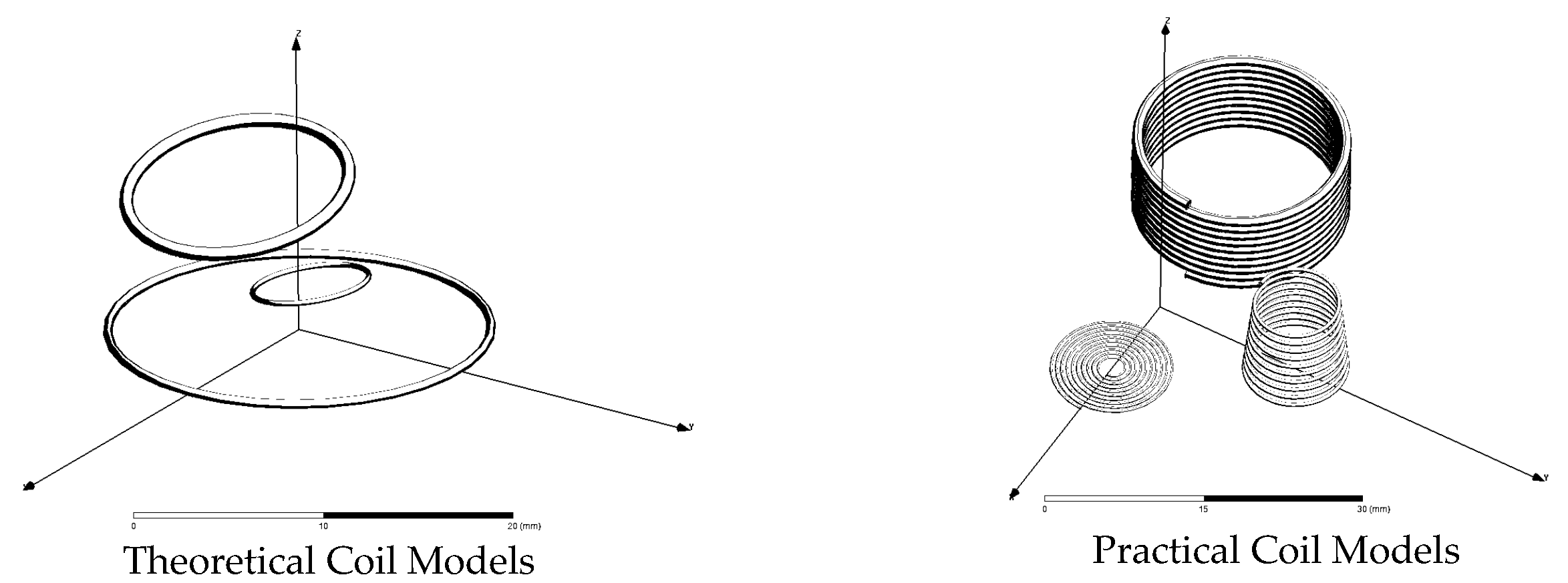
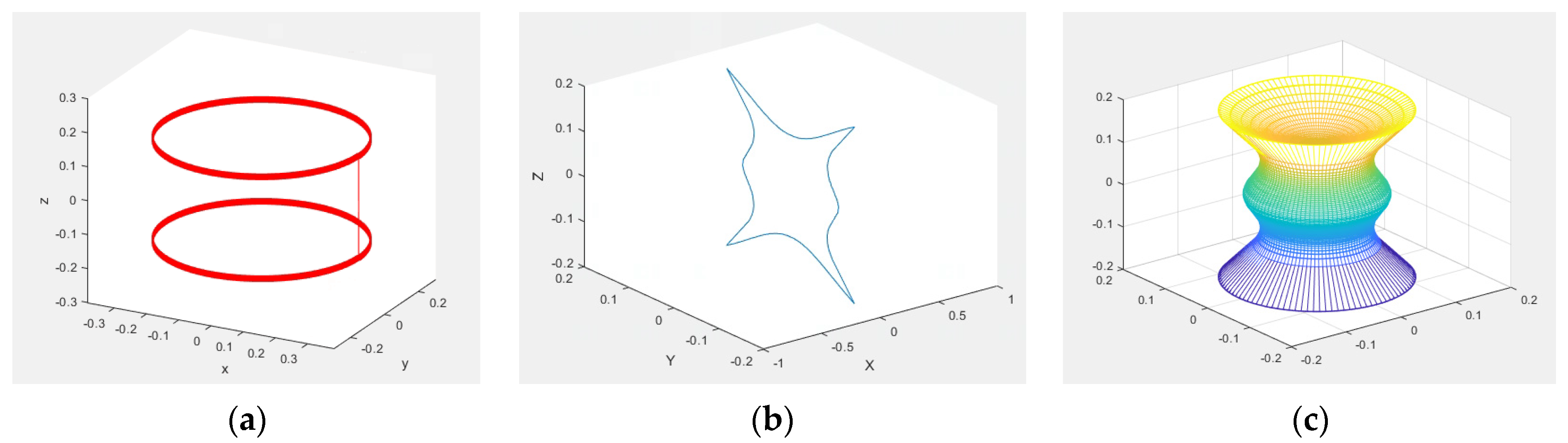
2.1. Winding Modelling

The winding trajectories are essentially defined as arrays of coordinates in 3 ; in other words, there are finite number of segments between these coordinates. Each segment length is set equal to the diameter of the wire—small enough for modelling any wire bended/wound into any shapes in real world. This is also required by the kernel function to achieve the best accuracy in calculation of the self-inductance [10]. However, it is recognized that when users apply parametric analysis, the enormous data initialization will be challenging, either defined manually or by programming. Therefore, we have proposed templates allowing users to generate windings using key points.

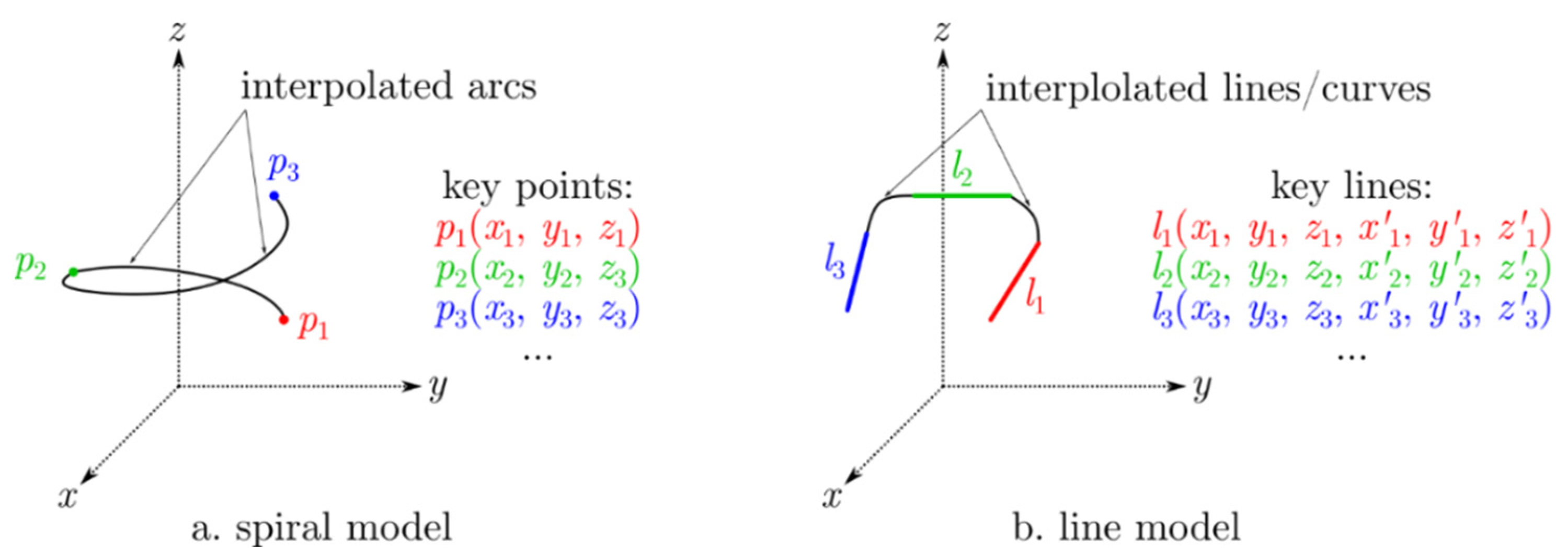
2.1.1. Spiral Type Windings

The template for spiral type coils is illustrated in Figure 4a. Any practical multi-turn circular, spiral or helical windings can be generated from a set of key points by interpolating arcs around z-axis. It is mostly easy using the cylindrical coordinate system to explain the interpolation method. Assuming that two points in Cartesian system p 1 ( x 1 , y 1 , z 1 ) and p 2 ( x 2 , y 2 , z 2 ) are converted into cylindrical representations p 1 ( r 1 , ϕ 1 ,   z 1 ) and p 2 ( r 2 , ϕ 2 ,   z 2 ) , and the interpolated arc will not exceed 2 π (no more than 1 turn), the smooth arc can be described using the function:
{ ϕ [ ϕ 1 ,   ϕ 2 ] ,       ϕ 1 < ϕ 2 r ( ϕ ) = ϕ ϕ 1 ϕ 2 ϕ 1 · ( r 2 r 1 ) + r 1 z ( ϕ ) = ϕ ϕ 1 ϕ 2 ϕ 1 · ( z 2 z 1 ) + z 1
Notice that it is also assuming ϕ 1 < ϕ 2 . In practice, the winding is wound via the key points in sequence and not necessarily guaranteeing this restraint. Therefore, if the next point’s angle ϕ is smaller than the previous one, a full turn should be added ( 2 π ). Using this method, both planar spiral windings and vertical helical windings can be represented in a unified way. It can also represent some irregular circular shapes neatly such as the hemispherical windings in a ball joint wireless power system [14]. Compared with the method using concentric circles to approximate a continuous multi-turn winding structure, the trajectories generated in this work are closer to the real-world windings especially when the pitch distance is significant compared with the thickness of the wire. The generated segmentation coordinates will be along the smooth arc (1), separated by identical length and the last segment will be trimmed, and the error cause by this trimming is neglectable.
All windings will be wound around z-axis during the first stage generation, but in many scenarios, they need to be simulated at a different position and angle. The windings can be later transformed with offset and rotated to certain angle.

2.1.2. Straight Line Type Model

In some other applications, rectangular shaped windings are often used [15], which require a different template. As shown in Figure 4b, the line-type windings can be generated from a series of lines with connections interpolated with lines or curves using the splines in the 3D space [16]. The segmentation method is similar to the spiral windings.

2.1.3. Preparations of the Winding Objects

All generated winding objects are uniformly stored in long arrays of coordinates with equal segment lengths of the wires’ corresponding diameters. An example representing a straight wire originated at 0 along x-axis with a diameter of a and N segments is shown in Table 1. As each segment has an equal length of a , the total length is N a and there are N + 1 coordinates in total.
The self- and mutual-inductance values can be calculated once all the segments of the windings are available and can be calculated using Neumann’s formula numerically [10]. The algorithm’s time complexity is O ( n 2 ) where n is the number of segments and this number is normally several thousand for commonly seen windings. Further, the total resistance can be quickly estimated as the total length of the wire is known. Depending on the type of wire used, solid wire and stranded wire will need to use different equations for skin-effect factors [17].

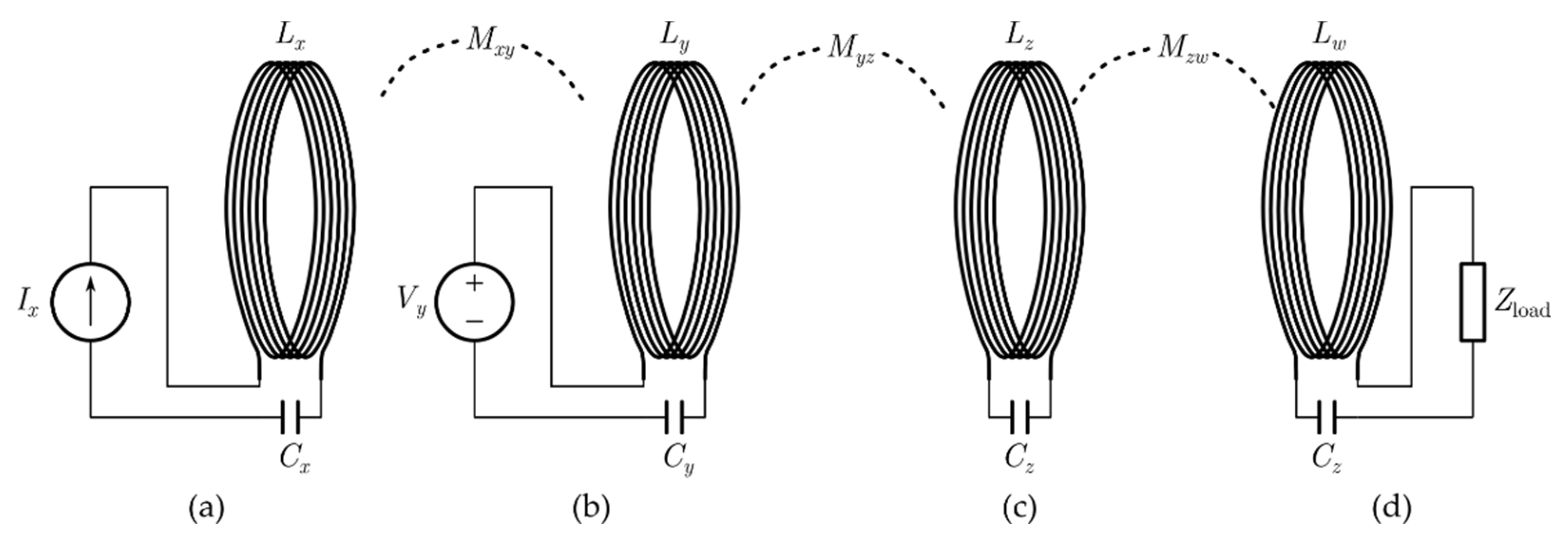
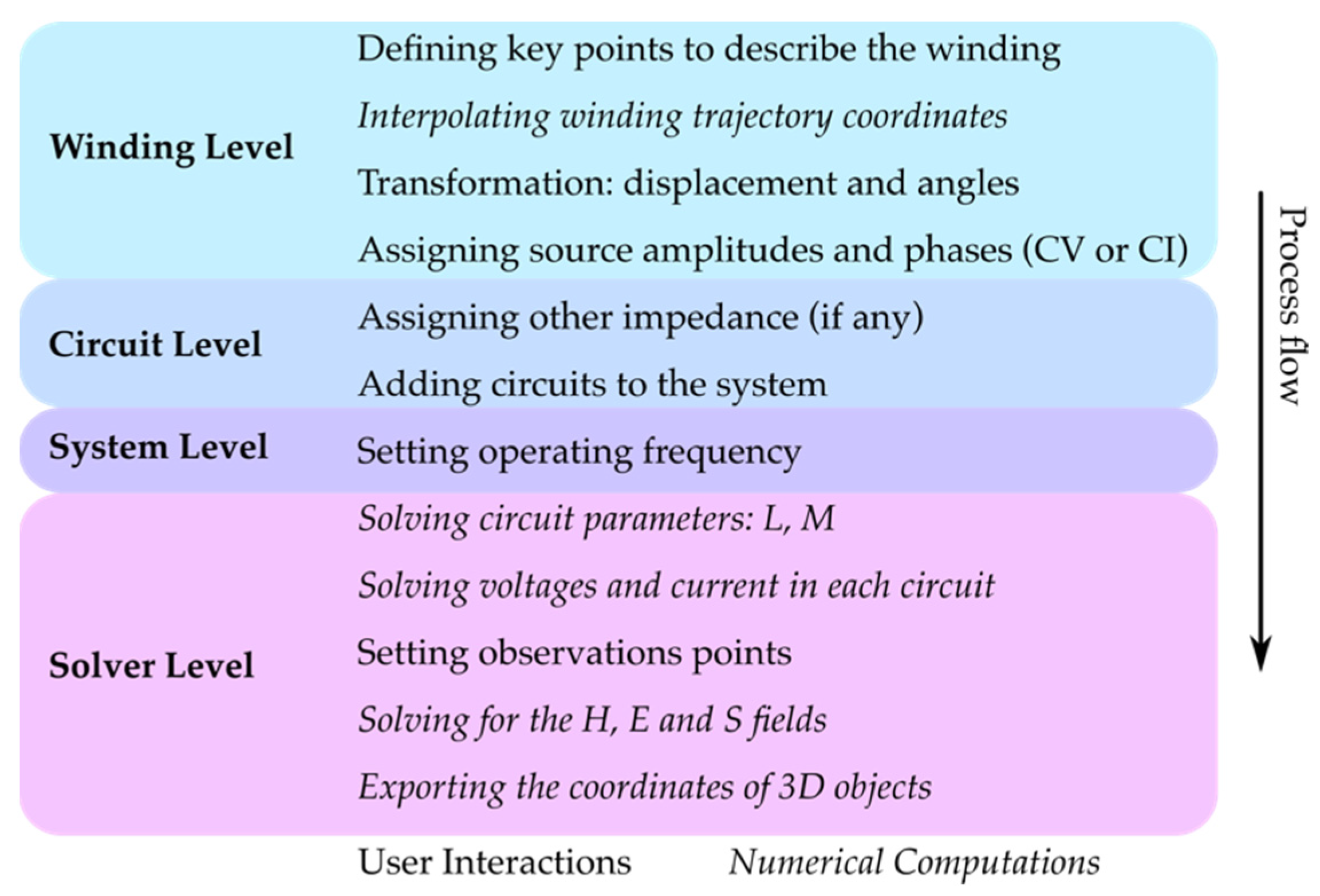
2.2. Circuit and System Modelling

The generated wire objects can be assigned to circuit objects, which also contain the sources, either a current source or a voltage source, and other passive components, for example, the compensation capacitance. An example of data structure is shown in Table 2. Then the circuit objects are added to a system object, which is a container for all the circuits and the simulation setups.

2.3. Solver

The solver calculates all the rest of the parameters and solves unknown values in the first step. All the winding resistances and inductance values can be calculated from the winding objects. For each circuit there will be at least one voltage restraint or current restraint. For voltage-restrained circuits, the current is to be solved, and vice versa. The solver needs an operating frequency ω to be set first. Assume that there are 1 n individual circuits (like those in Figure 2) in the system.
The general impedance equation is
[ R 1 + j X 1 j ω M 12 j ω M 13 j ω M 1 n j ω M 12 R 2 + j X 2 j ω M 23 j ω M 2 n j ω M 13 j ω M 23 R 3 + j X 3 j ω M 3 n j ω M 1 n j ω M 2 n j ω M 3 n R n + j X n ] [ I 1 I 2 I 3 I n ] = [ V 1 V 2 V 3 V n ]
where R x is the total series resistance, including the equivalent load impedance if any. X x is the total series reactance, including the reactance from the winding and compensation capacitance in the x th circuit. M x y is the mutual inductance between the x th and y th circuits. I x and V x are the current and the external voltage source in the x th circuit.
The matrix shall be reorganized and grouped into a submatrix equation separating CI sourced and CV sourced circuits. The rows representing current sources in Equation (2), having current values known and voltage values to be solved shall be swapped to the upper side of the equation, and rows representing voltage sources or no source (i.e., 0 voltage source) shall be moved downwards. The splitting borders between the two groups will divide (2) into the following equation.
[ U L U R L L L R ] [ I U I L ] = [ V U V L ]
where U L , U R , L L , L R are submatrices representing the impedances, I U are known current source values, V L are known voltage values (if they are voltage source driven, or 0 if no source is connected), and I L , V U are unknowns to be solved.
I L = L R 1 · ( V L L L · I U ) V U = U L · I U + U R · I L
All the calculations of physical quantities (except for coordinates) are complex numbers therefore amplitude and phase information are all retained, and both real and reactive power values are known.
The energy flow is visualized by rendered arrows on observation points distributed in space. The observation points can be sampled evenly over the three dimensions within the given ranges on x-, y-, and z-axis. The Poynting vector can be calculated using the method in [10] once all current amplitudes and phases are known in the system. This calculation is with a time complexity of O ( n × m × k ) where n is the number of segments, m is the scale of number of windings, and k is the scale of the observation points.
The codes are written in TypeScript and compiled and executed by NodeJS which is available on most platforms. The visualization results are rendered by WebGL which is now widely supported by modern web browsers including mobile platforms.

3. Results and Discussions

Three examples are shown here to demonstrate the versatility and convenience of this method.

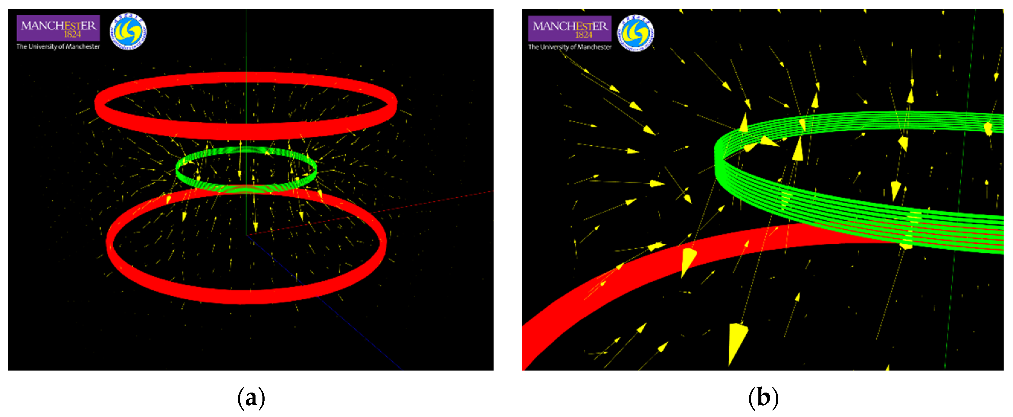
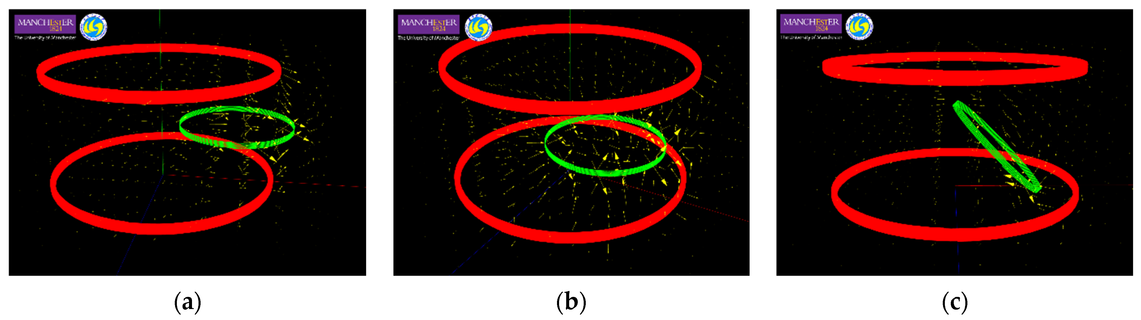
3.1. A Helmholtz Transmitter System

A Helmholtz coil consists of two concentric helical windings in series, but placed apart a certain distance and often used for applications requiring almost evenly distributed magnetic fields. Figure 5a shows the structure of a Helmholtz coil used as a transmitter for an IPT system, and Figure 5b,c shows the contour of an equal magnetic field strength. That the magnetic field near the center is contained though some nonideality is still quite obvious. As the two coils are connected in series, both parts are driven with the identical current. The operating frequency is 500 kHz.
Figure 6 shows the power flow in a Helmholtz-coil-transmitter wireless power transfer system. The transmitter winding is in red and the two parts are connected in series, with a diameter of 0.6 m, two layers and eight-turn-per-layer helical structure. The self-inductance of one half is 424.8 µH (as evaluated by IPTVisual) and is compensated with a capacitance of 0.2385 nF. The receiver winding is in green, with a diameter of 0.3 m, one layer of eight-turn-per-layer helical structure. The self-inductance is 45.5 µH (as evaluated by IPTVisual) and is compensated to the same frequency with a capacitance of 2.229 nF. A verification of the accuracy of the self- and mutual-inductance calculation of IPTVisual is in Appendix A. A 10 Ω load is applied to the receiver circuit. The execution time to get this 3D model by the NodeJS implementation on a desktop computer (i7-4790k, used single core@4GHz) is less than 2 min and memory consumption is less than 150 MB.
In Figure 7, the load circuit has been moved off the center. The power flow plots clearly demonstrate the spatial power density distributions. There are examples of coils moved to different places as well as tilted. Please note that while calculating all the Poynting vectors on the observation grids, all circuit parameters are known, which means that the current and power on the receiver side is pre-calculated. This method is also suitable for parametric optimizations. The calculation time is within seconds if the field data are not required, which can provide a time-efficient objective function solution for genetic-algorithm-based optimization applications.

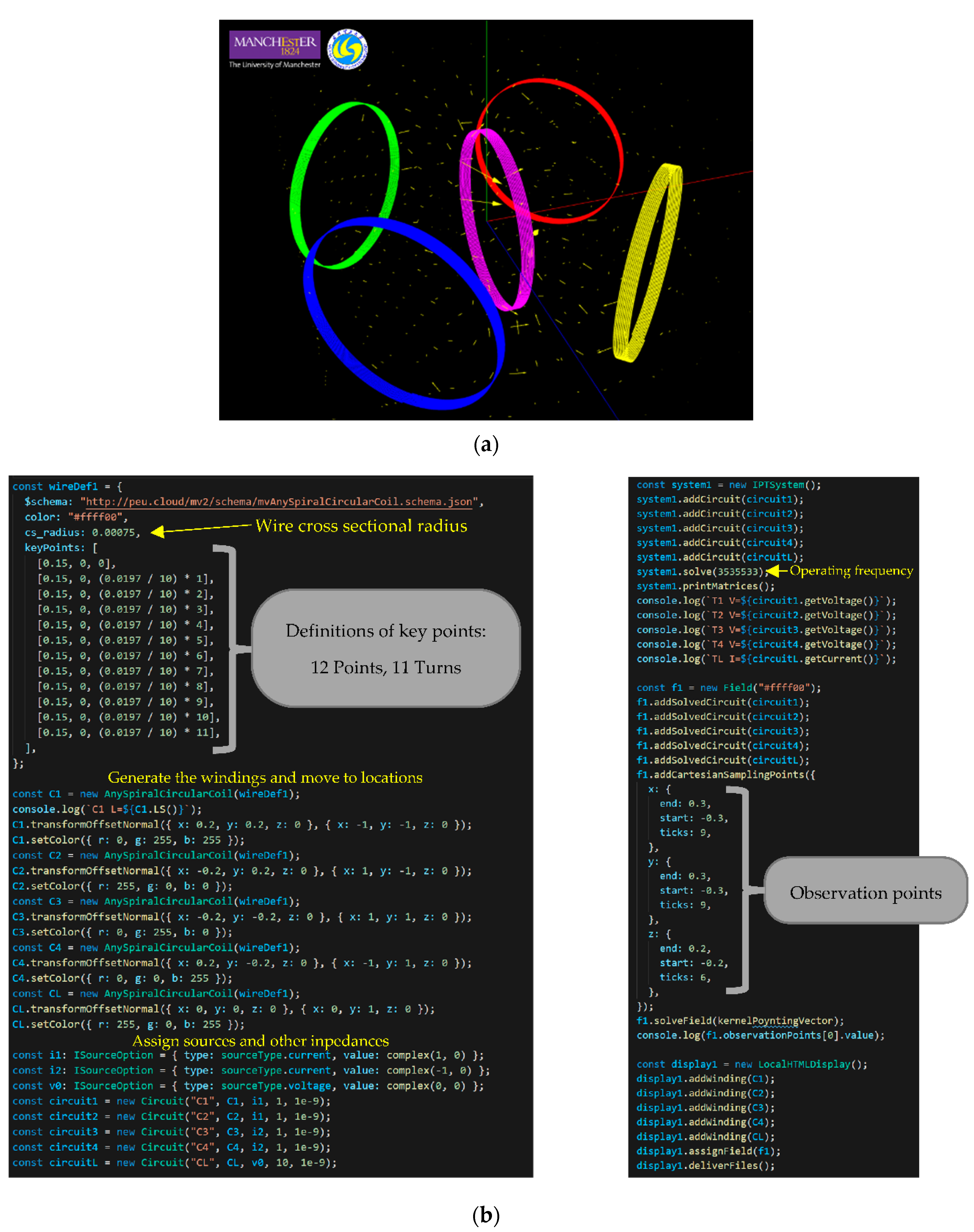
3.2. A Multi-Transmitter System

In Figure 8a, a 4-Tx-1-Rx IPT system (example in [18]) is simulated and the power flow is plotted. The proposed method flexibly supports versatile types of multi-winding wireless power transfer systems. A snapshot of the building codes to setup this simulation is shown in Figure 8b, where it can be seen that very little work is needed and most of the parameter settings are duplicated entries for multiple windings. This could greatly save the amount of time to establish a complicated IPT system with irregular shapes of windings, without trading off the computational time and complexity, as well as the flexibility of rearranging the circuits.

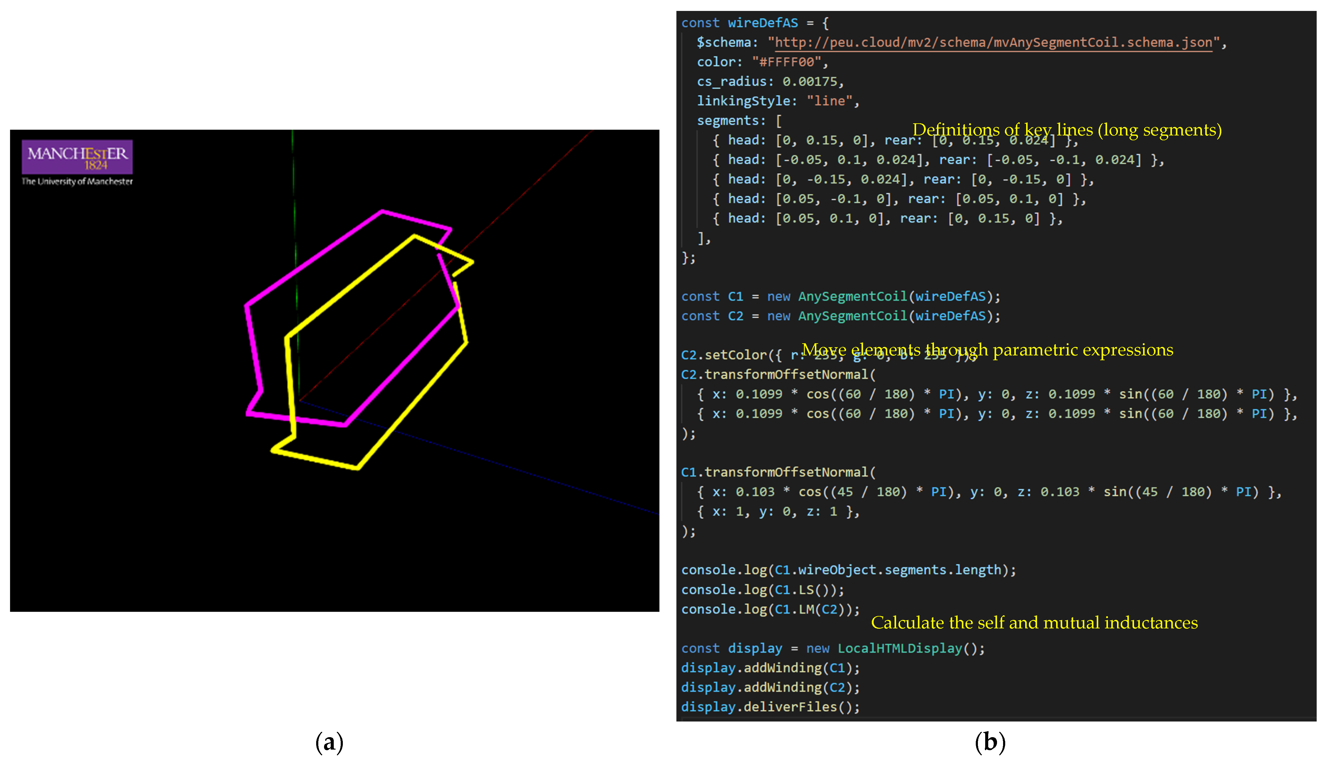
3.3. Line Windings Construction Used in Air-Core Electric Machines

In this example, as shown in Figure 9, a line winding model is used to build the air-core irregular shaped windings used in an air-core electric machine [19]. Only the impedance calculation is done in this example, as it is not a wireless power transfer system. Notice that only five lines of code are needed to define this coil shape.

4. Conclusions

An integrated numerical solver and visualizer for IPT wireless power transfer systems is proposed and developed, and the design and implementation details are explained in this paper. The amount of work required by users has been reduced to the minimum. In-detail winding trajectories, replicating real-world windings, can be generated from templates by specifying a few key points or lines. The windings can be transformed to arbitrary positions and angles. Both current and voltage excitation sources are supported and can be mixed. The execution time of the solver is acceptable on a typical computer. The generated results are in 3D models and can be rendered in a WebGL implemented webpage. This paper helps with the design and optimization of IPT systems and future automatic parametric search programs.

Author Contributions

Conceptualization, C.Z. and D.L.; methodology, C.Z., X.C.; software, C.Z. and K.C.; validation, X.C.; writing—original draft preparation, C.Z. and D.L.; visualization, C.Z.; supervision, D.L. All authors have read and agreed to the published version of the manuscript.

Funding

This research received no external funding.

Conflicts of Interest

The authors declare no conflict of interest.

Appendix A. Verification of the Self- and Mutual-Inductance Calculation in IPTVisual

Throughout the computation process, the accuracy of delivered quantities are all dependent on the evaluations of self- and mutual-inductance values from the given geometries. The performance (both in execution time and memory space) of the evaluation implementation is also critical to the usability for optimizations. In this section, we suggest some quick comparisons, to both analytical solutions and results from commercial FEM software (ANSYS) with standardized models.

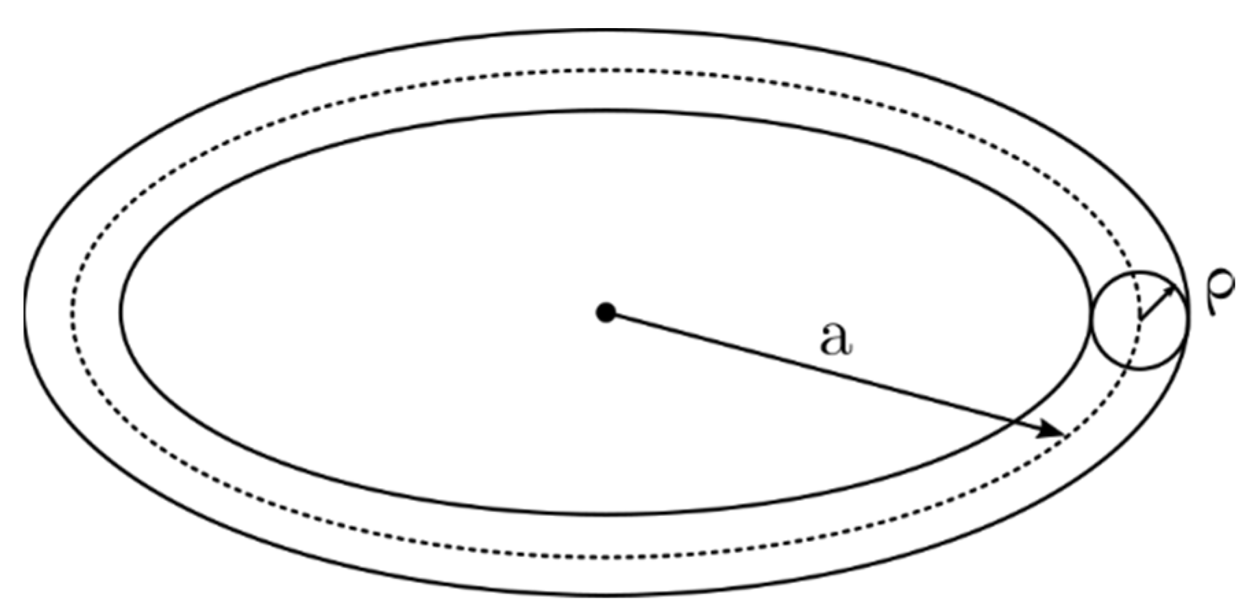
Appendix A.1. Self-Inductance of Circular Windings

A couple of self-inductance equations for single-turn circular windings are compared in [20]. As depicted in Figure A1, with a radius of a and a wire cross-section radius of ρ ,a self-inductance formula given by Maxwell is:
L = 4 π a ( ( 1 + 0.1137 ρ 2 a 2 ) log 8 a ρ 0.0095 ρ 2 a 2 1.75 )
which is recognized as one of the most accurate equations for a practically feasible winding.
Figure A1. Two parameters to define a simple circular winding.
Wevj 13 00063 g0a1
In an ANSYS simulation, the analysis setup is set to 1% error with the default meshing options. The circular winding model is generated by using the torus tool.
In IPTVisual, the model data is set as the following:
Cross-section radius:  ρ
Key-points: [( a , 0, 0), ( a , 0, 0)] … a full circle (arc) with radius a
The results are shown in Table A1. Both IPTVisual and ANSYS are run on the same computer (Intel i7-4790K, 16GB DDR3 RAM).
Table A1. Self-inductance of circular windings, using examples in [20].
Model ParametersEquation (A1)ANSYSIPTVisual (This Work, NodeJS)
a ρ L L TimeMem L TimeMem
0.25 m0.5 mm2.056 μH1.8097 μH102 min3.2 GB2.058 μH0.24 s48 MB
0.25 m5 mm1.333 μH1.0963 μH4.5 min2.3 GB1.323 μH0.20 s44 MB
0.10 m10 mm331.4 nH *310.7 nH1.5 min1.7 GB315.3 nH0.20 s40 MB
* In [20], this case is used to show the large errors with a large a / ρ ratio. Up to 9% difference is seen among all analytical formulae enumerated in this reference.
Obviously, general purpose FEM software is not capable of accurately predicting the inductance values due to the limitations on mesh granularity (especially the first one with a large a / ρ ratio, as it requires much finer mesh grids). The proposed method in IPTVisual, using fairly little time and memory, even when not optimized to its best, and the accuracy is good enough considering that the building dimensions and measurement error for practical windings will be inevitably large (estimated at least 10%).

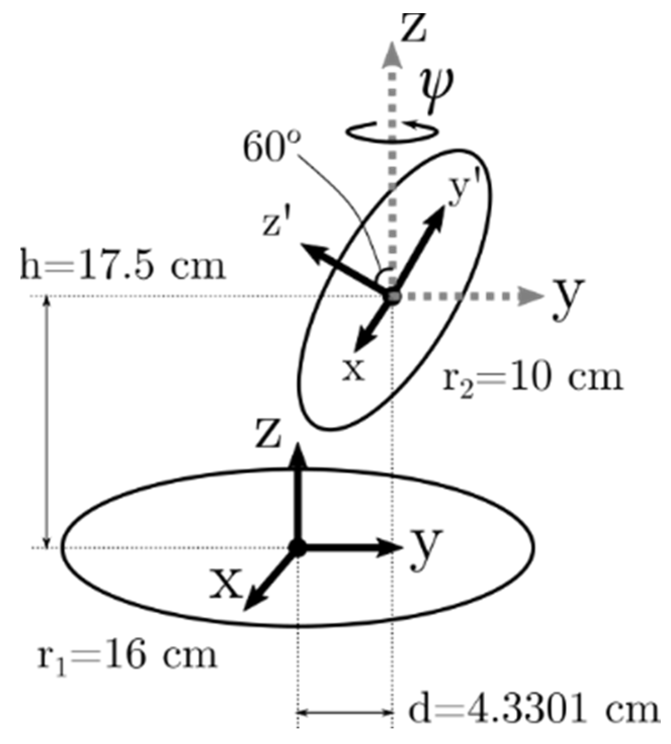
Appendix A.2. Mutual-Inductance between Two Circular Coils

In [21], examples of mutual-inductance calculations among two circular coils with variable displacement and angles are presented. The Example 12 with two tilting angles in [21] is used for verifying the accuracy and effectiveness of IPTVisual. There are also comparisons to FastHenry [22] results, and Grover’s formulae results in [23]. The model is set with two circular coils of 16 cm and 10 cm radii, respectively, and placed with a horizontal and vertical displacement of d = 4.3301 cm and 17.5 cm, respectively, as shown in Figure A2.
In IPTVisual, the model data is set as the following:
  • Cross-section radius: 5 μm … reference did not specify
  • C1 Key-points: [(0.16, 0, 0), (0.16, 0, 0)] … a full circle (arc) with radius 16 cm
  • C2 Key-points: [(0.10, 0, 0), (0.10, 0, 0)] … a full circle (arc) with radius 10 cm
  • C2 transform offset: (0, 4.3301, 17.5)
  • C2 transform normal: (sin(ψ)sin(60°), cos(ψ)sin(60°), cos(60°))
Figure A2. Lateral and angular misalignments in Example 12 in [21].
Wevj 13 00063 g0a2
The results are listed and compared in Table A2. On average, each mutual inductance calculation takes about 1 min and 160 MB RAM on a late-2021 MacBook Pro. The errors of IPTVisual result in analytical values that are even smaller than those of FastHenry, though the authors recognize both methods have very similar solver kernels, and the advancement may come from finer segmentations used in this work.
Table A2. Mutual-inductance between two circular windings, using examples in TABLE I in [21].
Azimuth Angle *Grover [23]Babic [21]FastHenry [22]IPTVisual
(This Work, NodeJS)
ψ M (nH) M (nH) M (nH) M (nH)
013.611313.611313.616213.6113
π/614.468814.468814.470414.4683
π/415.487715.487715.493215.4870
π/316.818916.818916.824916.8181
π/220.053420.053420.060420.0522
2π/323.325323.325323.333423.3238
3π/424.693624.693624.702224.6921
5π/625.749325.749325.758325.7478
π26.643326.643326.652626.6419
* The first half of the examples are shown here, the other half is mirrored due to symmetry.
The IPTVisual is developed for maximum flexibility and adaptivity and, therefore, implemented using JavaScript and run in the NodeJS environment. It is not optimized for the maximum performance, though the solving time is already fast enough for most simulations. A C++ implementation is expected to be 2× to 10× faster, and it is also possible to be developed into parallelized executables, on both multi-core CPUs and GPUs.

References

  1. Consortium, W.P. Wireless Power Consortium. Available online: https://www.wirelesspowerconsortium.com/ (accessed on 25 February 2021).
  2. Rahman, M. Motorola Demos Wireless Charging Tech That Can Power Devices 100cm Away. Available online: https://www.xda-developers.com/motorola-no-contact-wireless-charging/ (accessed on 29 January 2021).
  3. Araque, J. Xiaomi Introduces a Wireless Charger That Can Charge Your Phone from Two Meters Away. Business Insider. 2 February 2021. Available online: https://www.businessinsider.com/xiaomi-charger-mobile-distance-wireless-remote-technology-smartwatch-testing-advance-mi-air (accessed on 25 February 2021).
  4. Cheah, W.; Watson, S.A.; Lennox, B. Limitations of wireless power transfer technologies for mobile robots. Wirel. Power Transf. 2019, 6, 1–15. [Google Scholar] [CrossRef] [Green Version]
  5. Shin, J.; Song, B.; Lee, S.; Shin, S.; Kim, Y.; Jung, G.; Jeon, S. Contactless power transfer systems for On-Line Electric Vehicle (OLEV). In Proceedings of the 2012 IEEE International Electric Vehicle Conference, Greenville, SC, USA, 4–8 March 2012. [Google Scholar]
  6. Shinohara, N. Novel Beam-Forming Technology for WPT System to Flying Drone. In Proceedings of the 2020 IEEE Wireless Power Transfer Conference (WPTC), Seoul, Korea, 15–19 November 2020. [Google Scholar]
  7. Hui, R.S.Y.; Zhong, W.; Lee, C.K. A Critical Review of Recent Progress in Mid-Range Wireless Power Transfer. IEEE Trans. Power Electron 2014, 29, 4500–4511. [Google Scholar] [CrossRef] [Green Version]
  8. Energous Receives FCC Approval, Extending Charging Zone to up to 1 Meter for Groundbreaking Over-the-Air, Power-at-a-Distance Wireless Charging. Business Wire. 30 September 2020. Available online: https://www.businesswire.com/news/home/20200930005275/en/Energous-Receives-FCC-Approval-Extending-Charging-Zone-to-Up-to-1-Meter-for-Groundbreaking-Over-the-Air-Power-at-a-Distance-Wireless-Charging (accessed on 25 February 2021).
  9. Zhang, C.; Zhong, W.; Hui, R.S.Y.; Liu, X. A time-efficient methodology for visualizing time-varying magnetic flux patterns of mid-range wireless power transfer systems. In Proceedings of the 2013 IEEE Energy Conversion Congress and Exposition, Denver, CO, USA, 15–19 September 2013. [Google Scholar]
  10. Wang, H.; Zhang, C.; Hui, R.S.Y. Visualization of Energy Flow in Wireless Power Transfer Systems. In Proceedings of the 2019 IEEE Wireless Power Transfer Conference (WPTC), London, UK, 18–21 June 2019. [Google Scholar]
  11. Liu, Y.; Hu, A.P.; Madawala, U. Determining the power distribution between two coupled coils based on Poynting vector analysis. In Proceedings of the 2017 IEEE PELS Workshop on Emerging Technologies: Wireless Power Transfer (WoW), Chongqing, China, 20–22 May 2017. [Google Scholar]
  12. Faria, J.A.B. Poynting Vector Flow Analysis for Contactless Energy Transfer in Magnetic Systems. IEEE Trans. Power Electron. 2012, 27, 4292–4300. [Google Scholar] [CrossRef]
  13. Furusato, K.; Imura, T.; Hori, Y. Multi-band coil design for wireless power transfer at 85 kHz and 6.78 MHz using high order resonant frequency of short end coil. In Proceedings of the 2016 International Symposium on Antennas and Propagation (ISAP), Okinawa, Japan, 24–28 October 2016. [Google Scholar]
  14. Zhang, C.; Lin, D.; Hui, R.S.Y. Ball-Joint Wireless Power Transfer Systems. IEEE Trans. Power Electron. 2018, 33, 65–72. [Google Scholar] [CrossRef]
  15. Ho, G.K.Y.; Zhang, C.; Pong, B.M.H.; Hui, R.S.Y. Modeling and Analysis of the Bendable Transformer. IEEE Trans. Power Electron. 2016, 31, 6450–6460. [Google Scholar] [CrossRef]
  16. Schumaker, L.L. Spline Functions: Computational Methods; Society for Industry and Applied Mathematics: Philadelphia, PA, USA, 2015. [Google Scholar]
  17. Sullivan, C.R. Optimal choice for number of strands in a litz-wire transformer winding. IEEE Trans. Power Electron. 1999, 14, 283–291. [Google Scholar] [CrossRef] [Green Version]
  18. Zhang, C.; Lin, D.; Hui, R.S.Y. Efficiency optimization method of inductive coupling wireless power transfer system with multiple transmitters and single receiver. In Proceedings of the 2016 IEEE Energy Conversion Congress and Exposition (ECCE), Milwaukee, WI, USA, 18–22 September 2016. [Google Scholar]
  19. Jin, Z.; Iacchetti, M.F.; Smith, A.C.; Deodhar, R.P.; Komi, Y.; Abduallah, A.; Umemura, C. Winding Inductance Estimations in Air-Cored Resonant Induction Machines. In Proceedings of the 2020 IEEE Energy Conversion Congress and Exposition (ECCE), Detroit, MI, USA, 11–15 October 2020. [Google Scholar]
  20. Rosa, E.B.; Cohen, L. On the self-inductance of circles. In Bulletin of the Bureau of Standards, Department of Commerce and Labor; US Department of Commerce and Labor: Washington, DC, USA, 1908; Volume 4. [Google Scholar]
  21. Babic, S.; Sirois, F.; Akyel, C.; Girardi, C. Mutual Inductance Calculation between Circular Filaments Arbitrarily Positioned in Space: Alternative to Grover’s Formula. IEEE Trans. Magn. 2010, 46, 3591–3600. [Google Scholar] [CrossRef]
  22. Kamon, M.; Tsuk, M.J.; White, J. FASTHENRY: A multipoleaccelerated 3-D inductance extraction program. IEEE Trans. Microw. Theory Tech. 1994, 42, 1750–1758. [Google Scholar] [CrossRef]
  23. Grover, F.W. Inductance Calculations; Dover: New York, NY, USA, 1964. [Google Scholar]
Figure 1. Differences between theoretical and practical coil models.
Wevj 13 00063 g001
Figure 2. Typical resonance circuits in IPT systems: (a) driven by ac current source; (b) driven by ac voltage source; (c) undriven, used as relay resonator; (d) undriven, with an external load.
Wevj 13 00063 g002
Figure 3. Process flow of the proposed method.
Wevj 13 00063 g003
Figure 4. Winding generation templates: (a) spiral model; (b) line model.
Wevj 13 00063 g004
Figure 5. (a) Structure of the Helmholtz coil; (b) YOZ plot of the equal magnetic field contour; (c) 3D plot of the equal magnetic field contour.
Wevj 13 00063 g005
Figure 6. (a) Power flow in a Helmholtz coil transmitter IPT system with load placed at centre; (b) enlarged area showing the Poynting vectors are greater near the load (green) winding and flowing into it.
Wevj 13 00063 g006
Figure 7. (a) Power flow when the load is horizontally offset 20 cm from the centre; (b) power flow when the load is displaced down 5 cm and left 10 cm; (c) power flow when the receiver in (b) is tilted to 45 degrees.
Wevj 13 00063 g007
Figure 8. (a) Power flow in a 4-Tx-1-Rx IPT system, which was proposed in [17]; (b) a snapshot of the codes needed to build this simulation.
Wevj 13 00063 g008
Figure 9. (a) Modelled irregular shaped windings; (b) a snapshot of the codes.
Wevj 13 00063 g009
Table 1. An example of the data structure for a straight piece of wire.
PropertyTypeData
DiameterNumbera
Number of coordinatesNumberN + 1
CoordinatesListAddressData
0<0, 0, 0>
1<a, 0, 0>
N<Na, 0, 0>
Table 2. An example of the data structure for a circuit object.
PropertyTypeContent
WindingObjectReference to winding object
Source TypeEnum{CV|CI |Null} *
Source ValueComplex NumberSource amplitude and phase
Compensation ImpedanceComplex NumberTotal series impedance
* CV: constant voltage source; CI: constant current source; Null: no source, used as relay or load.
Publisher’s Note: MDPI stays neutral with regard to jurisdictional claims in published maps and institutional affiliations.

