Article

Adaptive Pre-Aim Control of Driverless Vehicle Path Tracking Based on a SSA-BP Neural Network

Guangxi Key Laboratory of Auto Parts and Vehicle Technology, School of Electrical Electronics and Computer Science, Guangxi University of Science and Technology, Liuzhou 545006, China
*
Author to whom correspondence should be addressed.
World Electr. Veh. J. 2022, 13(4), 55; https://doi.org/10.3390/wevj13040055
Submission received: 19 February 2022 / Revised: 11 March 2022 / Accepted: 17 March 2022 / Published: 22 March 2022

Abstract

:
Aiming at the problem that the tracking accuracy of unmanned vehicle path tracking preview control is greatly affected by the preview time, a BP neural network adaptive preview control method is proposed. Considering that the prediction effect of the BP neural network is limited to the initial value setting, a preview time adjuster based on the SSA-BP neural network was established; by establishing the relationship between the front wheel steering angle and the preview time, a new direction control driver model was formed. The driver model and the preview time adjuster together constitute an adaptive steering controller. In order to solve the influence of the longitudinal speed change on the vehicle stability, a PID variable-speed controller was designed to realize the horizontal and vertical coordinated control of the path tracking of the unmanned vehicle. Compared with the fixed preview time and the BP preview time control method, the results show that the proposed method has strong tracking ability when driving at various speeds on three consecutive curves and Alt 3 test roads, and can be used when driving at a variable speed.

1. Introduction

Driverless vehicles represent the key development direction of automobiles, and the path tracking control is one of the key technologies needed in order to realize the accurate path tracking and planning of driverless vehicles and ensure their safe and stable driving [1,2]. In the study of path tracking control, the control methods can be divided into pre-aim and non-pre-aim, according to the source of external information. In non-pre-aim control, a composite control strategy was used to design the path-tracking controller [3,4]; in order to solve the problem of accurate tracking in curves, an adaptive control method was applied [5]. Furthermore, in order to solve the problem of vehicle rollover caused by excessive roll angle during cornering, a roll angle constraint was added to the model predictive controller design to achieve the limitation of body roll angle, but the impact of the vehicle’s nonlinear characteristics on stability was not considered [6]. Most of the above studies use the feedback principle approach, which usually does not consider the driver’s predictive role in the “human–vehicle–road” system for vehicle maneuvering behavior. However, human drivers are used to making reasonable driving decisions by observing the road ahead during the driving process [7].
Pre-aim control is a path-tracking control method based on the driver model that integrates the driver’s forward view of the path with the estimation of the vehicle motion state, and is one of the main research directions in driverless vehicles [8]. According to the different types of tasks, the driver models can be divided into directional control driver models, speed control driver models, and speed directional control driver models [9]. In [10], the optimal pre-aim theory was proposed for the first time, and the driver’s pre-aim role was considered in the path-tracking controller design, which is simple in structure, easy to implement, and has high control accuracy. Five driver models were proposed based on the driver pre-aim theory using different assumptions, each with its own focus on the control effect [11]. The trajectory pre-aim controller was designed using the trajectory feedforward + vehicle state feedback method to improve the tracking accuracy when the vehicle dynamically changes lanes [12]. The arc length pre-aim method was proposed to improve the robustness and computational speed of the pre-aim controller [13]. The above methods do not take into account the tracking characteristics of real drivers, and cannot take into account safety, stability, and comfort at the same time. The pre-aim distance and time are key parameters in the pre-aim control theory, and the above study designed them as fixed and constant parameters, which will produce the problem of poor adaptability and poor tracking effect of tracking control for complex driving conditions [14].
The authors of [15] designed a pre-aim distance adaptive tracking controller based on the pre-aim angle deviation, which achieved more accuracy in a tracking task when the initial deviation was large, but only for low-speed conditions. Furthermore, by analyzing the influence of parameters on the path-tracking effect during the driving process, the variable weight multipoint pre-aim method was used to improve the stability under the low-adhesion-coefficient road surface [16,17]; the variable pre-aim distance controller was designed according to the current vehicle speed using fuzzy rules [18], based on which the influence of road curvature was considered to design the dual pre-aim point transverse–longitudinal controller, in order to complete the tracking task of the vehicle within a safe speed range under the large curvature path [19]. Fuzzy control mostly uses the operating behavior of skilled drivers to develop fuzzy rules and, in order to eliminate the influence of human factors, adaptive optimization is used to achieve dynamic adjustment of the pre-aim distance [20]. On study analyzed the influence of vehicle speed and road curvature on the tracking path, and proposed a particle swarm optimization (PSO) pre-aim control method to achieve adaptability to complex road conditions [21]. The author of [22] investigated the relationship between pre-aim time and road curvature, and proposed a selection method that provided a new research direction to study control-variable pre-aim time control; meanwhile, other studies used driving deviation to design an optimization function to adaptively select pre-aim time [23,24]. The authors of [25] proposed adaptive pre-aim time based on a BP neural network, and this method can reduce the lateral cumulative tracking error under different driving modes, but its control effect is limited by the influence of the initial value of the BP neural network. BP neural networks have the advantages of nonlinearity, fault tolerance, and adaptivity but, due to the disadvantages of the large influence of the initial value on the training effect and the tendency to fall into local optimization, their prediction accuracy is not high enough when used as predictors in some specific applications. Therefore, intelligent algorithms such as genetic algorithms (GAs) [26,27], particle swarm optimization (PSO) [28,29], and cuckoo search (CS) [30] are used to optimize the initial weights and thresholds of BP neural networks.
This paper establishes a new directional control driver model based on the theory of pre-aim control and the design of a decision mechanism based on the deviation relationship between the current position and the pre-aim point. We used the sparrow search algorithm to optimize the initial value of the BP neural network and improve its prediction accuracy, so as to establish the SSA-BP neural network pre-aim time adjuster. Considering that the change in the vehicle’s longitudinal speed has a great influence on the tracking effect, the current longitudinal acceleration was solved by a PID algorithm to achieve the control of vehicle speed. We built a combined simulation model with CarSim and Simulink to verify the effectiveness of the SSA-BP-neural-network-based path tracking adaptive pre-aim controller.

2. Vehicle Model

The influence of the steering system on the vertical direction of the vehicle is small when the vehicle is driven on a dry road. To simplify the analysis, a two-degrees-of-freedom vehicle model with lateral tilt and a transverse pendulum was chosen as the reference model in this paper, and its differential equations are as follows:
β ˙ = 2 C f   +   C r m v x β 1 + 2 C f l f     C r l r m v x 2 ω + 2 C f m v x δ f ω ˙ = 2 C r l r     C f l f I z β 2 C f l f 2     C r l r 2 v x I z ω + 2 C f l f I z δ f
where v x is the longitudinal vehicle speed, β is the lateral deflection angle of the center of mass, ω is the angular velocity of transverse swing, δ f is the front wheel angle, m is the vehicle weight, I z is the rotational inertia, C f and C r are the lateral deflection stiffness of the front and rear tires, respectively, and l f and l r are the distances from the front and rear axles, respectively, to the center of mass of the vehicle.
Selecting state vectors x   =   β ; ω and u = δ f , the vehicle state space expression is as follows [11]:
x ˙ = 2 C f   +   C r m v x 2 C r l r     2 C f l f m v x 2 1 2 C r l r     C f l f I z 2 C f l f 2   +   C r l r 2 I z v x x + 2 C f m v x 2 C f l f I z u

3. SSA-BP-Neural-Network-Based Adaptive Pre-Aim Control for Path Tracking

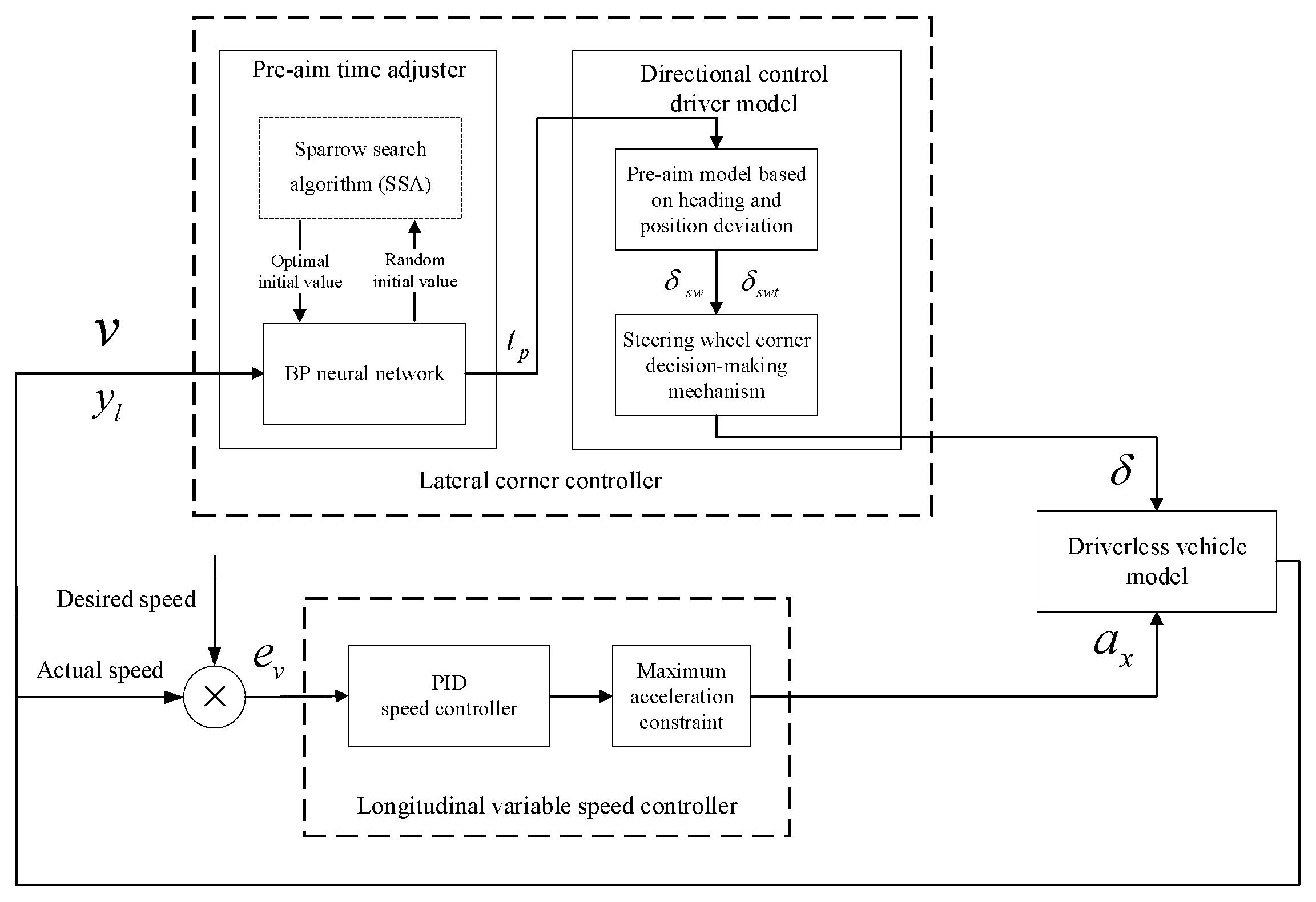
3.1. Overall Control Scheme

The SSA-BP-neural-network-based adaptive pre-aim control scheme for unmanned vehicle path tracking is shown in Figure 1, and consists of a lateral corner controller and a longitudinal variable-speed controller. The lateral corner controller includes the SSA-BP neural network pre-aim time adjuster and a driver direction control model. The pre-aim time adjuster is used to achieve an accurate path-tracking effect, and the pre-aim time is predicted dynamically based on the vehicle’s state information (vehicle speed v , pre-aim distance y l ) at the current moment using the BP neural network. The initial values of the BP neural network are optimized offline using the sparrow search algorithm (SSA) to overcome the problem that the network is susceptible to local minima due to the nonlinear characteristics of the vehicle, and to obtain the initial weights and thresholds for optimization. The driver direction control model includes a pre-aim control model based on the driving position and heading deviation of the vehicle, and solves for the current steering wheel angle δ of the vehicle through the steering wheel turn decision mechanism. Since the change in longitudinal speed will have an impact on the path tracking when the vehicle is driving on the actual road, the longitudinal variable-speed controller is established by using a PID control algorithm. The longitudinal speed error e v is adjusted according to the principle of fast and smooth tracking of the target speed, and the desired longitudinal acceleration a x is calculated, while the acceleration is limited in order to avoid the occurrence of rapid speed change, and the longitudinal speed change function of the vehicle is realized under the premise of ensuring the comfort of the ride.

3.2. Directional Control Driver Model

3.2.1. Pre-Aim Control Model

The human driver is constantly making decisions based on the curvature of the road and the current steering wheel rotation angle during the driving process, which follows the following relationship:
ρ = δ s w i s w L
where ρ is the road curvature, δ s w is the steering wheel rotation angle, i s w is the vehicle’s steering system ratio, and L = l f + l r is the wheelbase.
Figure 2 shows the optimal curvature model of the relative vehicle–road position; f t is the desired trajectory of the road, and the vehicle travels to the desired point C after pre-aim time t p .
The lateral displacement of the vehicle at moment t 0 + t p is:
y t 0 + t p   =   y t 0   +   t p y ˙ t 0   +   t p 2 2 y ¨ t 0
The lateral acceleration is:
y ¨ t 0   =   v 2 R = v 2 ρ
where R   is the turning radius of the vehicle.
Combining Equations (4) and (5) yields the road curvature:
ρ = 2 y t 0 + t p     y t 0     t p y ˙ t 0 v t p 2
Substituting Equation (6) into Equation (3) yields:
δ s w = 2 i s w L y t 0 + t p     y t 0     t p y ˙ t 0 v t p 2
Equation (7) gives the steering wheel angle calculated based on the deviation of the center of mass of the vehicle from the pre-aim point, without considering the transient angular deviation of the vehicle at that point.
Figure 3 shows the prediction model of vehicle trajectory under constant transverse pendulum angular velocity; x o y is the vehicle coordinate system, X O Y   is the geodesic coordinate system, point G is the vehicle’s center of mass, point M   is the circle center of the pre-aim path, y l is the lateral distance between the pre-aim point C and the vehicle’s center of mass, x v and y v are the vehicle displacements along the x   and y   directions, respectively, and the combined velocity of v = v x 2 + v y 2 vehicles is kept constant. Assuming that the unmanned vehicle runs to the pre-aim point C at time   t p   , the angular velocity of the transverse pendulum is constant, and there is no lateral position deviation during the motion, the vehicle moves in a uniform circular motion, and its combined velocity direction is tangential to the desired path.
According to the geometric relationship yielding C G A = C G B + β , by the definition of the chord tangent angle we can know that C G B = θ 2 , so C G A = θ 2 + β to get the vehicle center of mass and the lateral distance y l of the pre-aim point.
y l = tan θ 2 + β x v
The vehicle moves in a uniform circular motion to obtain a circular angle θ .
θ = ω t p
Vehicle longitudinal displacement x v :
x v = v x t p
From Equation (9), the ideal angular velocity of the vehicle’s transverse pendulum ω t :
ω t = θ t p
Substituting the above equation into Equation (8) gives:
ω t = 2 tan 1 y l x v β t p
The vehicle moves in a uniform circular motion during the pre-aim time, and the vehicle is in a steady state, i.e., x ˙ = 0 .
β ˙ = 0 ω ˙ = 0
Substituting the above equation into Equation (2) yields the steady-state gain G ω of the theoretical transverse pendulum angular velocity ω t versus steering wheel rotation angle δ s w .
G ω = v x i s w L 1 + K v x 2
where the vehicle stability factor k = m l r C r     l f C f 2 C r C f L 2 .
The ideal steering wheel turning angle δ s w t under consideration of angular deviation is obtained by combining Equations (12) and (14):
δ s w t = ω t G ω = 2 tan 1 y l v x t p     β t p G ω

3.2.2. Steering Wheel Cornering Decision Mechanism

In Figure 2, l 1 is the current heading and l 2 is the heading at the pre-aim point. e a is the deviation of the heading from the current position to the presight point—negative clockwise and positive counterclockwise. e p is the deviation of the position from the center of mass to l 2 —negative left and positive right. The human driver makes steering decisions by observing position deviation e p and heading deviation e a together, so the design of the driver model also requires dynamic selection based on both. If the two can cancel one another out, the vehicle is in equilibrium and the control output is zero; conversely, control is performed according to the following decision method:
δ   =   δ m a x + δ m i n e a   +   e p 2 e a e a   +   e p + e p e a   +   e p 1 2 , δ s w + δ s w t 0 0 , δ s w + δ s w t = 0
where δ m a x = m a x δ s w , δ s w t ,   δ m i n = m i n δ s w , δ s w t .
In summary, the driver model depends mainly on the forward-looking role of the pre-aim control, and the pre-aim model takes the road state at the pre-aim point as the basis for estimation, according to Equations (7) and (15), so the control amount is directly related to the pre-aim time. When actually driving, drivers will take different pre-sighting times for different road conditions. In this study, the SSA-BP neural network pre-aim time adjuster described in Section 3.3 was used to simulate the pre-aim time selection law of human drivers in different driving environments, and the directional driver control model was established according to Equation (16).

3.3. SSA-BP Neural Network Pre-Aim Time Adjuster

3.3.1. BP Neural Network

The BP neural network adjusts the corresponding weights and thresholds according to the fastest gradient descent method to minimize the total network error; it mainly consists of an input layer, an implicit layer, and an output layer. The number of neurons in the hidden layer is set according to the following equation:
q = j + k + a
where q is the number of neurons in the hidden layer, j and k are the number of neurons in the input and output layers, respectively, and a is a random number between 1 and 10.
In this study, the BP neural network was applied to predict the pre-aim time values under different vehicle states, and a 2-5-1 network structure was used. The input quantities were the current vehicle speed and the pre-aim distance, and the output quantity was the pre-aim time in a certain vehicle state. The sigmoid function was used for the excitation function of the nodes in the implicit layer, the purelin function was used for the excitation function of the nodes in the output layer, the mean square error function (MSE) was used for the performance function, the maximum number of iterations was 100, the training result error was set to 0.00001, and the learning efficiency was set to 0.01.

3.3.2. Sparrow Search Algorithm (SSA)

The sparrow search algorithm (SSA) is a population intelligence optimization method based on the foraging and anti-predation behavior of sparrow populations [31]. The authors of [32] used standard test functions to verify the performance of the SSA algorithm; the results showed that it outperforms conventional algorithms such as particle swarm algorithms and gray wolf optimization algorithms in terms of accuracy, convergence speed, and avoidance of becoming trapped in local optimization. Applying SSA to optimize the initial weights and thresholds of the BP neural network offline, the first step is to obtain the dimension j of the optimization problem for the SSA calculation based on the BP neural network structure, and to set the number of iterations and the sparrow size as follows:
j = R N + N + N L + L
where R is the number of input nodes, N is the number of implied nodes, and L is the number of output nodes.
The absolute value of the total prediction error generated by the random initial weights and thresholds of the BP neural network is chosen as the sparrow fitness value, as follows:
f i t n e s s = s u m a b s p b
where p is the predicted output value of the network and b is the actual output value of the network.
Sparrow populations are divided into discoverers and joiners, with discoverers usually having easier access to food sources and providing foraging direction for the entire population; joiners obtain food by following discoverers. The identity of the two is dynamic, but the proportion of the population is constant. The smaller the fitness value in the SSA, the stronger the predation ability, so the finder has a wider search area than the joiner, and its location update is described as follows:
X i , j t + 1   =   X i , j t e x p i α i t e r m a x , R 2 S T X i , j t + Q L , R 2 > S T
where t represents the current number of iterations, i is the number of sparrows, j is the dimensionality of the optimization problem, X i , j t denotes the positional information of the t -th optimization of the i -th sparrow in the j -th dimension, and i t e r m a x denotes the maximum number of iterations. α     0 , 1 is a random number, R 2     0 , 1 denotes the warning value, and S T     0.5 , 1 denotes the safety value—0.8 was chosen for this paper. R 2 < S T indicates that the population is in a safe state and can search for food in a wide area; R 2 S T indicates the presence of a predator around an individual, and informs the whole population to abandon the search and fly to a safe area immediately. Q is a random number subject to normal distribution, and L is an all-one matrix of 1 × d .
Some accessions with poor foraging locations are more likely to fly to other locations to forage for more food sources. The updated descriptions of the accessions’ locations are as follows:
X i , j t + 1   =   Q e x p X w o r s t     X i , j t i 2 , i > n 2 X i , j t + 1   +   X i , j t X p t + 1 A + L , i n 2
where X p is the optimal position currently occupied by the discoverer, X w o r s t denotes the current global worst position, A is a 1 × d matrix with each element being 1 or −1, and A + = A T A A T 1 ; i > n 2 indicates that the i -th accession with a lower fitness value is not getting food, is starving, and needs to fly to other places to forage for more food.
Ten percent of individuals were selected for vigilance work, and the entire population was in an anti-predatory state when in danger. The location of the vigilantes was updated and described as follows:
X i , j t + 1   =   X b e s t t + τ X i , j t X b e s t t , f i > f g X i , j t + H X i , j t     X w o r s t t f i     f w + ε , f i = f g
where X b e s t is the current global optimal position, τ is a normal random number obeying a 0–1 distribution as the control step parameter, H     1 ,   1 is a random number, f i , f g , and f w denote the current individual sparrow fitness value and the current global best and worst fitness values, respectively, and ε is a constant to prevent the denominator from being zero, which was set to 10 e 10 in this study.

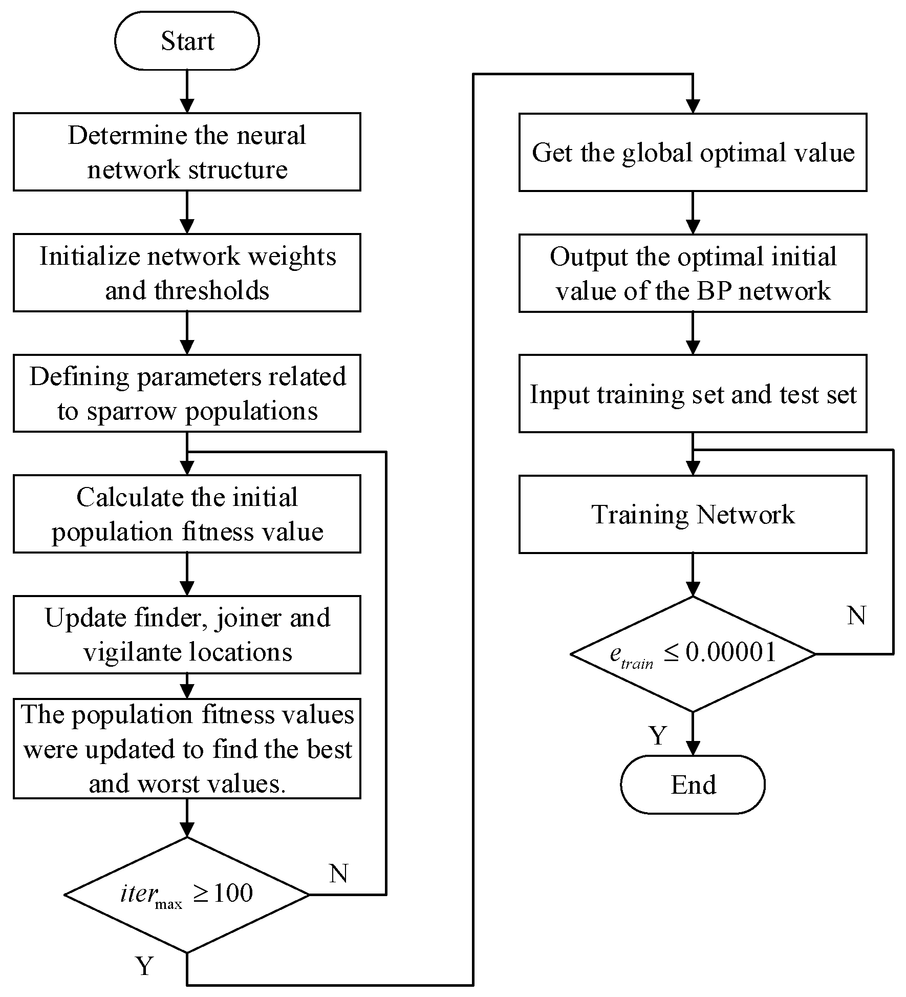
3.3.3. Pre-Aim Time Adjuster

The training process of BP neural networks often treats the characteristics of training samples as general properties, making it prone to overfitting and leading to large training errors, and the training effect depends heavily on the selection of initial weights and thresholds. To solve the above problems, the initial values of the BP neural network were optimized offline using the SSA algorithm described in Section 3.3.2, and the optimization results were used for network training. The optimized results can effectively prevent the BP neural network from falling into the problem of local minima due to improper initial value selection, and can improve the convergence speed at the same time.
The SSA-BP neural network algorithm flow is shown in Figure 4, and the steps are as follows:
  • Firstly, the topology of the BP neural network and the input and output variables are determined, and the algorithm stopping condition is set as the maximum error value e t r a i n e 4 ;
  • The weights and thresholds of the BP neural network are initialized, and the parameters related to the SSA algorithm, such as ( i t e r m a x , τ , S T , etc.), are defined;
  • The fitness values of the sparrow population are calculated and ranked from smallest to largest to find the current optimal and worst values, where the initial fitness value is the training error of the random initial value of the BP neural network;
  • Equations (20)–(22) are used to update the location of finders, joiners, and vigilantes, respectively;
  • The optimal value of the sparrow position for this iteration is obtained, and the position is updated if the new position is better than the optimal value of the previous iteration; otherwise, no position update is performed;
  • If the maximum number of iterations i t e r m a x = 100 is reached, the search is stopped, and the global optimum and the best fitness value are output; otherwise, steps 3–5 are repeated;
  • The parameters corresponding to the global optimum of the SSA algorithm are used as the initial weights and thresholds of the BP neural network, and the network is trained by inputting training and testing sample sets.
Because the trained BP neural network is used to predict the pre-aim time, the established SSA-BP neural network is a pre-aim time adjuster. The actual vehicle speed and pre-aim distance information in each control cycle are input to obtain different pre-aim times for various vehicle states, and the process is shown in Figure 5.

4. Simulation Experiments and Analysis

In order to verify the effectiveness of the proposed method (hereafter: the method in this paper) for path tracking under complex conditions such as continuous large-curvature curves and variable-speed driving, continuous three-curve roads and Alt 3 test roads were selected for experiments. The joint simulation model was built in CarSim and Simulink, the vehicle was selected as the experimental vehicle from CarSim, and the SSA-BP neural network pre-aim time regulator model was built in Simulink. This was compared with the fixed pre-aim control method (hereafter referred to as method 1), the BP neural network adjusted pre-aim control method with random initial values (hereafter referred to as method 2), and the GWO-BP neural network pre-aim control method (hereafter referred to as method 3).
Using the direction-controlled driver model described in Section 3.2, different vehicle speeds, pre-aim distances, and pre-aim times were selected to perform tracking experiments on the reference path (U-turn path), and 20,012 sets of data with tracking errors within ±0.2 m of the pre-targeting control were used as training samples to train the SSA-BP neural network. The network training target was reached after 29 iterations with fast convergence; 53 sets of test samples were used to test the SSA-optimized network, and the results are shown in Figure 6. As can be seen from Table 1, the improved algorithm has a mean absolute error (MAE) of 2.059 × 10 3 a root-mean-square error (RMSE) of 2.29 × 10 2 , and a maximum error of 6.156 × 10 2 . This pre-aim time regulator has high prediction accuracy; it can reduce the accumulated deviation caused by understeering during high-speed turns and improve the adaptability to cope with complex working conditions.

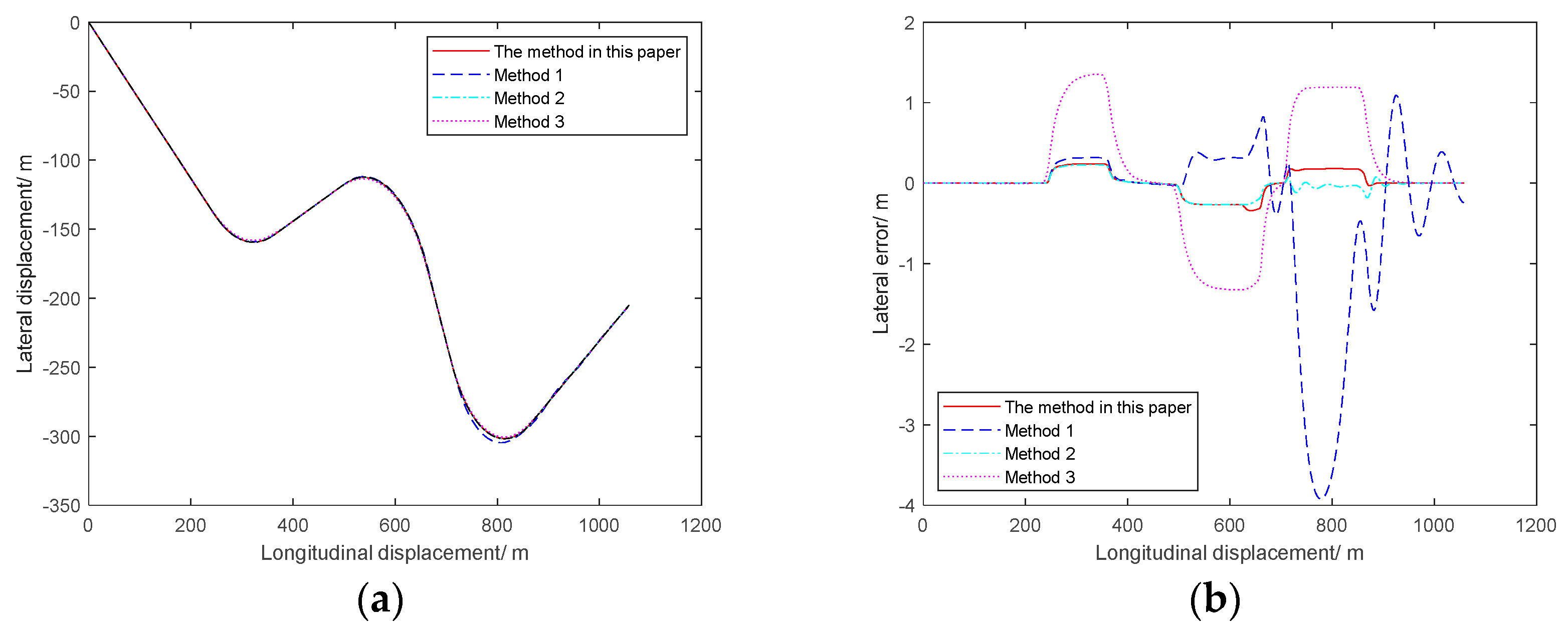
4.1. Variable-Speed Continuous Three-Curve Roads Tracking Experiment

In this section, the experimental road was composed of three U-bends, the vehicle was set to drive on dry road, and the speed was set to 36 km/h for 0–410 m and 72 km/h for 410–820 m, after which the vehicle was accelerated to 108 km/h. Thus, the vehicle was simulated to drive from the city to the full speed range, and the experimental results are shown in Figure 7. As seen in Figure 7a, the longitudinal variable-speed controller has fast tracking capability for the target speed, and the rise time is shorter when switching from low-speed to medium-speed than when switching from medium-speed to high-speed driving, which can quickly approach and converge to the target speed. Combined with the lateral error variation results in Figure 7c, this shows that improving the lateral stability of the vehicle comes at the expense of the longitudinal speed of the vehicle. During the actual control of the vehicle, the longitudinal velocity is not precisely controlled to the desired value. This is due to the fact that the PID controller output is the desired longitudinal acceleration, and due to the nonlinearity and complexity of vehicle dynamics during high-speed turns, the actual value deviates from the desired value, but it does not have a significant impact on the overall tracking control performance because it does not break the control logic of the system, and the actual value can be kept close to the desired value by adjusting the controller parameters to meet the desired longitudinal control performance.
As shown in Figure 7b, the average lateral error of the method in this paper is only 8.538 e 4 m under various speed conditions, with a high tracking accuracy. The tracking error of method 1 increases continuously with the increase in the vehicle’s speed; the lateral error reaches 0.4826 m at 847 m, the oscillation phenomenon appears when the transition is to straight driving, and at 108 km/h it has seriously deviated from the target trajectory, and the phenomenon of “drawing 8” appears. Method 2 can achieve accurate tracking at both low and medium speeds, but when the acceleration increases to 108 km/h, affected by the BP neural network falling into local minima, the prediction accuracy of the pre-aim time decreases, the foresight of road changes is insufficient, and the vehicle suffers from steering lag and oscillation at the exit of the curve, which seriously reduces the stability of the vehicle. Method 3 is limited by the prediction accuracy of the pre-aim time regulator, resulting in the inability to implement the path-tracking task. As seen in Figure 7c, the lateral errors of the method in this paper at the bend are 0.1747 m, 0.2204 m, and 0.1184 m, respectively, and the accumulated lateral errors can be cancelled out in the second half of the bend by the driver’s forward-looking action after the change in direction, indicating that the pre-targeting time-adaptive control can reduce the lateral tracking errors and achieve the effect of accurate tracking under the variable-speed conditions. Figure 7d shows the adaptive change in the pre-aim time of the method in this paper, and it can be seen that the pre-aim time takes different values at different driving speeds, which can adapt to the changes in the external environment by selecting different control parameters according to the vehicle driving information and help to achieve accurate tracking under variable-speed conditions.

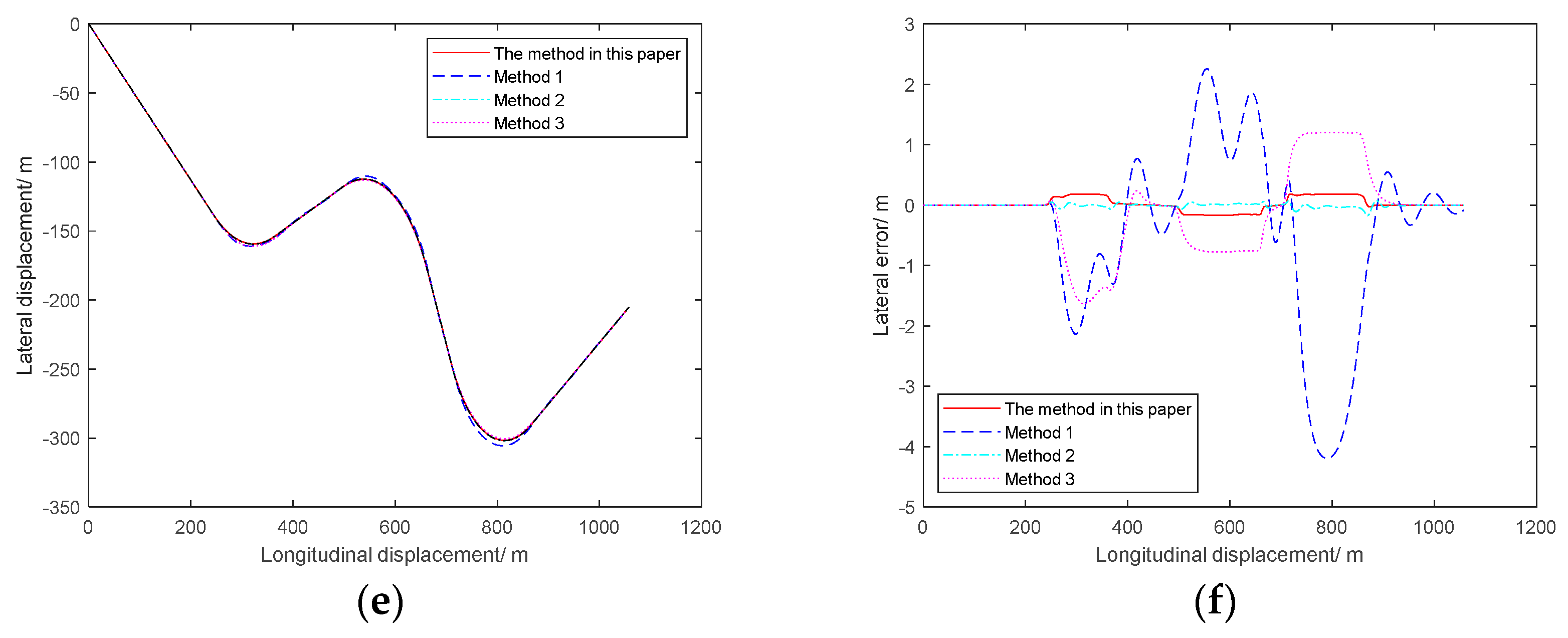
4.2. Alt 3 Road Tracking Experiment

The Alt 3 road is a test road incorporating a horizontal slope and a front-to-back slope, which can comprehensively evaluate the path-tracking controller performance. Figure 8 shows the simulation results of the Alt 3 test road under different speed conditions. As can be seen from Figure 8a, the driving trajectories of the three methods overlap with the target path when the vehicle speed is 36 km/h, and all have a better tracking effect. At 72 km/h, lateral error is increased; from Figure 8d it can be seen that the error direction of method 1 and this paper’s method, method 2, and method 3 is not consistent; this paper’s method takes control of the vehicle on the curve at the first turn, indicating that the driver model can pre-aim the road curvature changes and steering control, and the maximum lateral error is 34% less than in method 1—only 0.3175 m. The vehicle controlled by method 1 takes a period of time to stabilize to zero after exiting the curve, increasing the chance of vehicle instability. At 108 km/h the method in this paper has a predictive effect on vehicle speed and road changes, the lateral error variation range is −0.1689 to 0.1842 m, and because the SSA-optimized neural network has high prediction accuracy, it makes the lateral error at high speeds significantly lower than that at low and medium speeds, significantly improving the tracking accuracy under high-speed conditions. Method 2 has insufficient prediction ability for large-curvature roads (at the second and third curves), fails to anticipate steering in advance, and fails to compensate for lateral coupling errors caused by longitudinal speed changes, resulting in body sway. Method 3 seriously deviates from the lane, and loses tracking ability.
Furthermore, the tracking performance of the method in this paper was verified under variable-speed conditions. The vehicle was set to drive on a dry road at a speed of 36 km/h for 0–410 m, 72 km/h for 410–670 m, and finally accelerate to 108 km/h. Figure 9 shows the Alt 3 test road simulation results under variable-speed conditions. The method in this paper eliminates the accumulated error during driving by adaptively changing the pre-aim time under variable-speed conditions, which not only improves the path-tracking accuracy, but also reduces the chance of vehicle instability. The vehicle controlled by method 1 has a smoother tracking curve at the first curve, but at the exit of the second curve under the dual influence of vehicle acceleration and steering lag, the vehicle has a lateral error of 3.922 m and deviates from the road. Method 2 still has high tracking accuracy at low and medium speeds, but the tracking error fluctuates more at high speeds, and the stability of the controlled vehicle is insufficient.

5. Conclusions

Considering the influence of pre-aim time on path tracking in the path tracking pre-aim control model of unmanned vehicles, this paper constructed an SSA-BP neural network pre-aim time adjuster under complex road conditions and variable speed conditions to achieve the adaptive change of pre-aim time and obtain a path tracking adaptive pre-aim control method.
The main conclusions obtained in this paper are as follows.
  • Based on the vehicle model and the pre-aim control model, we built a “human–vehicle–road” closed-loop control system and proposed a new directional control driver model;
  • The offline optimization of BP neural network primaries by the sparrow search algorithm (SSA) improves the prediction accuracy of the pre-aim time. Considering the law of pre-aim time selection under different driving conditions, the controller established by using the directional control driver model was used to conduct simulation experiments on the reference path (U-turn path). The SSA-BP neural network was trained with the obtained parameter samples to achieve the dynamic selection of pre-aim time;
  • The longitudinal variable-speed controller was designed to reduce the coupling effect of longitudinal speed on path tracking, making the method in this paper more adaptable to a wide range of speed variation and able to achieve accurate path tracking under a variety of variable-speed working conditions;
  • Through the tracking simulation experiments on two different roads, the results show that the maximum error value of the method in this paper is only 0.2673 m under the fixed-speed and variable-speed conditions, providing a new scheme for the research of path tracking pre-scanning control.
The proposed pre-aim time adjuster in this paper is only related to the vehicle speed and pre-aim distance during the driving process, and does not consider the road adhesion coefficient, which will be considered in subsequent studies to make it more consistent with actual situations.

Author Contributions

Conceptualization, Y.H. and W.L.; methodology, Y.H.; software, Y.H.; validation, Y.H., W.L. and H.L.; formal analysis, Y.H.; investigation, Y.H.; resources, Y.H.; data curation, Y.H.; writing—original draft preparation, Y.H.; writing—review and editing, Y.H.; visualization, Y.H.; supervision, Y.H. and H.L.; project administration, Y.H.; funding acquisition, W.L. All authors have read and agreed to the published version of the manuscript.

Funding

This research was funded by Guangxi Natural Science Foundation Key Projects, grant number 2020GXNSFDA238011, the Open Fund Project of Guangxi Key Laboratory of Automation Detection Technology and Instrument, grant number YQ21203, and an Independent Research Project of Guangxi Key Laboratory of Auto Parts and Vehicle Technology, grant number 2020GKLACVTZZ02.

Institutional Review Board Statement

Not applicable.

Informed Consent Statement

Not applicable.

Data Availability Statement

Not applicable.

Conflicts of Interest

The authors declare no conflict of interest. The funders had no role in the design of the study; in the collection, analyses, or interpretation of data; in the writing of the manuscript, or in the decision to publish the results.

References

  1. Bellotti, F.; Kim, S.W.; Lian, F.L. Introduction to the Special Issue on Applications and Systems for Collaborative Driving. IEEE Trans. Intell. Transp. Syst. 2017, 18, 3457–3460. [Google Scholar] [CrossRef]
  2. Martinez, C.M.; Heucke, M.; Wang, F.Y.; Gao, B.; Cao, D. Driving Style Recognition for Intelligent Vehicle Control and Advanced Driver Assistance: A Survey. IEEE Trans. Intell. Transp. Syst. 2017, 19, 666–676. [Google Scholar] [CrossRef] [Green Version]
  3. Park, M.; Lee, S.; Han, W. Development of Steering Control System for Autonomous Vehicle Using Geometry-Based Path Tracking Algorithm. ETRI J. 2015, 37, 617–625. [Google Scholar] [CrossRef]
  4. He, H.; Shi, M.; Li, J.; Cao, J.; Han, M. Design and experiential test of a model predictive path following control with adaptive pre-aim for autonomous buses. Mech. Syst. Signal Processing 2021, 157, 107701. [Google Scholar] [CrossRef]
  5. Citlalli, G.S.; Yassine, R. Dynamic Speed Adaptation for Path Tracking Based on Curvature Information and Speed Limits. Sensors 2017, 17, 1383. [Google Scholar]
  6. Hong, S.; Hedrick, J.K. Roll prediction-based optimal control for safe path following. In Proceedings of the American Control Conference, IEEE, Chicago, IL, USA, 1–3 July 2015; pp. 3261–3266. [Google Scholar]
  7. Cao, J.; Lu, H.; Guo, K.; Zhang, J. A Driver Modeling Based on the pre-aim-Follower Theory and the Jerky Dynamics. Math. Probl. Eng. 2013, 2013, 1–10. [Google Scholar]
  8. Gang, C.; Su, S.H. Driver-behavior-based robust steering control of unmanned driving robotic vehicle with modeling uncertainties and external disturbance. Proc. Inst. Mech. Eng. Part D J. Automob. Eng. 2020, 234, 1585–1596. [Google Scholar]
  9. Chen, T.; Li, X.; Sun, L.; Wei, L. Review and Prospect of Driver Model in Intelligent Vehicle Design. Automob. Technol. 2014, 6, 1–6. [Google Scholar]
  10. Guo, K. Modeling of Driver/Vehicle Directionl Control System. Veh. Syst. Dyn. 1993, 22, 141–184. [Google Scholar] [CrossRef]
  11. Chen, W.; Tan, D.; Wang, H.; Wang, J.; Xia, G. A kind of driver direction control model based on trajectory prediction. J. Mech. Eng. 2016, 52, 106–115. [Google Scholar] [CrossRef]
  12. Zhi-Gen, N.; Wan-Qiong, W.; Wei-Qiang, Z.; Zhen, H.; Chang-Fu, Z. Dynamic trajectory planning and tracking control of smart car lane changing based on trajectory pre-aim. J. Traffic Transp. Eng. 2020, 20, 147–160. [Google Scholar]
  13. Li, S.; Xu, Y.H.; Chen, J.; Zhu, P.X. Research on Vehicle Lateral Tracking Control Based on Arc Length pre-aim. Automot. Eng. 2019, 41, 668–675. [Google Scholar]
  14. Zhang, L.Z.; Guan, H.; Jia, X.; Lu, P.P.; Chen, Y.S. A Study on the Effect of Driver Model Parameters on the Performance of Driver-Vehicle-Road Closed-Loop System. Appl. Mech. Mater. 2014, 470, 604–608. [Google Scholar] [CrossRef]
  15. Wang, H.; Wang, G.; Luo, X.; Zhang, Z.; Gao, Y.; He, J.; Yue, B. Tracking control method of agricultural machinery navigation path based on pre-aim tracking model. Trans. Chin. Soc. Agric. Eng. 2019, 35, 11–19. [Google Scholar]
  16. Li, Y.H.; Liu, Y.; Feng, Q.L.; Nan, Y.F.; He, J.; Fan, J.C. Intelligent commercial vehicle path following control based on optimal pre-aim and model prediction. J. Automot. Saf. Energy 2020, 11, 462–469. [Google Scholar]
  17. Sun, M.X.; Man, X.M.; Wang, J.H.; Wang, J.H.; Guo, D.; Man, X.H. Overtaking path tracking control based on dynamics and pre-aim theory. J. Shandong Univ. Technol. (Nat. Sci. Ed.) 2021, 35, 33–38. [Google Scholar]
  18. Jiang, J.X.; Shi, P.L.; Zhou, L.H.; Zhang, L. Smart car path tracking control with variable pre-aim distance. J. Shandong Univ. Technol. (Nat. Sci. Ed.) 2021, 35, 70–74, 80. [Google Scholar]
  19. Diao, Q.Q.; Zhang, Y.N.; Zhu, L.Y. Horizontal and vertical fuzzy control of large curvature path for smart car with dual pre-aim points. China Mech. Eng. 2019, 30, 1445–1452. [Google Scholar]
  20. Chen, W.W.; Wang, J.E.; Wang, M.L.; Wang, J.B. Adaptive pre-aim Control of Lateral Movement of Intelligent Vehicles with Vision Navigation. China Mech. Eng. 2014, 25, 698–704. [Google Scholar]
  21. Zhao, Z.G.; Zhou, L.J.; Zhu, Q. Adaptive optimization of pre-aim distance for unmanned vehicle path tracking control. J. Mech. Eng. 2018, 54, 166–173. [Google Scholar] [CrossRef]
  22. Li, Y. Direction and Speed Integrated Control Driver Model and Its Application in ADAMS. Master’s Thesis, Jilin University, Changchun, China, 2008. [Google Scholar]
  23. Jin, X.Y.; Zhang, J.; Liu, Y.S.; Wang, Q.S. Research on adaptive optimal pre-aim model based on Stanley algorithm. Comput. Eng. 2018, 44, 42–46. [Google Scholar]
  24. Li, H.Z.; Li, L.; Song, J.; Yu, L.Y.; Wu, K.H.; Zhang, X.L. Optimal pre-aim driver model with adaptive pre-aim time. J. Mech. Eng. 2010, 46, 106–111. [Google Scholar]
  25. Xie, J.; Jiang, H.B.; Ma, S.D. Adaptive analysis of pre-aim time of smart car driver model. J. Jiangsu Univ. (Nat. Sci. Ed.) 2018, 39, 254–259. [Google Scholar]
  26. Ran, Y.Q.; Wu, W.; Di, X. Research on Pipe Network Leakage Location Model Based on Genetic Algorithm Optimized BP Neural Network. Water Resour. Power 2021, 39, 123–126, 122. [Google Scholar]
  27. Chai, Y.; Li, T.; Zhang, L. Production Forecast of Coalbed Methane Based on GA Optimized BP Neural Network. In Proceedings of the 2019 IEEE 4th Advanced Information Technology, Electronic and Automation Control Conference (IAEAC), IEEE, Chengdu, China, 20–22 December 2019. [Google Scholar]
  28. Long, Y.; Deng, X.L.; Yang, X.X.; Hou, Z.X. Short-term rapid prediction of stratospheric wind field based on PSO-BP neural network. J. Beijing Univ. Aeronaut. Astronaut. 2021. [Google Scholar] [CrossRef]
  29. Pang, X.; Ma, H.; Su, P.; Tang, G.Y. TPPMA: New Adaptive BP Neural Network Based on PSO and PCA Algorithms. In Proceedings of the 2018 IEEE 27th International Symposium on Industrial Electronics (ISIE), Cairns, QLD, Australia, 13–15 June 2018. [Google Scholar]
  30. Xie, L.X.; Wang, Z.H. Network security situation assessment method based on cuckoo search optimization BP neural network. J. Comput. Appl. 2017, 37, 1926–1930. [Google Scholar]
  31. Xuan, J.K. Research and application of a new type of swarm intelligence optimization technology. Donghua Univ. Xuan Jiankai 2020. Available online: https://cdmd.cnki.com.cn/Article/CDMD-10255-1020647458.htm (accessed on 20 February 2022).
  32. Xue, J.; Shen, B. A novel swarm intelligence optimization approach: Sparrow search algorithm. Syst. Sci. Control Eng. 2020, 8, 22–34. [Google Scholar] [CrossRef]
Figure 1. Block diagram of adaptive pre-aim control of path tracking based on an SSA-BP neural network.
Wevj 13 00055 g001
Figure 2. Optimal curvature model of relative vehicle–road position.
Wevj 13 00055 g002
Figure 3. Vehicle trajectory prediction model under constant yaw rate.
Wevj 13 00055 g003
Figure 4. SSA-BP neural network algorithm flowchart.
Wevj 13 00055 g004
Figure 5. SSA-BP neural network pre-aim time adjuster workflow.
Wevj 13 00055 g005
Figure 6. Test sample verification results: (a) Comparison of predicted values and true values. (b) Predicted error values.
Wevj 13 00055 g006
Figure 7. Variable-speed continuous-curve simulation results: (a) Longitudinal speed change curve of the vehicle. (b) Path tracking with different methods. (c) Lateral displacement tracking deviation. (d) Adaptive change in pre-aim time.
Wevj 13 00055 g007
Figure 8. Alt 3 simulation results at different speeds: (a) 36 km/h path-tracking effect. (b) 36 km/h lateral tracking error. (c) 72 km/h path-tracking effect. (d) 72 km/h lateral tracking error. (e) 108 km/h path-tracking effect. (f) 108 km/h lateral tracking error.
Wevj 13 00055 g008aWevj 13 00055 g008b
Figure 9. Simulation results of variable speed on the Alt 3 road: (a) Variable-speed path-tracking effect. (b) Variable-speed lateral tracking error.
Wevj 13 00055 g009
Table 1. Performance comparison of different pre-aim time regulators.
AlgorithmMaximum ErrorMAERMSE
BPNN0.13620.015830.047
GWO-BPNN0.075540.0049890.02331
SSA-BPNN0.061560.0020590.0229
Publisher’s Note: MDPI stays neutral with regard to jurisdictional claims in published maps and institutional affiliations.

