Analysis and Research on Power Supply Strategies of Electric Vehicles Based on Wind Farms

Abstract

The widespread growth of electric vehicles could pose significant grid and charging infrastructure challenges, especially in areas with underdeveloped infrastructure. This has affected the ease of charging electric vehicles. In this paper, I design a power supply strategy for electric vehicle charging facilities based on wind farm power supply. In this strategy, a preliminary selection of line conductors is carried out, and several schemes are preliminarily determined. Further comparative analysis is made from the three aspects of conductor, tower type, and bus. Through the PowerWorld software, a simulation model is established for each scheme, and an optimal strategy that takes into account economy, security, and system stability is obtained (AAC 31.5 mm double split, tower A and bus 5). This can assist in the transformation of electric vehicle power supply and the construction of wind farm power supply facilities.

1. Introduction

Energy is the cornerstone of the development of the automobile industry, and energy also affects the degree of development of the automobile industry [1]. Energy is crucial for social development. Even in a modern society with the development of science and technology, the world’s energy source is conventional energy. New energy [2] is gradually becoming the backbone of future electric vehicle development [3].

New energy technology will be a key factor affecting people’s work and lives in the future. With the gradual exhaustion of fossil energy [4] and the aggravation of pollution, people begin to pay attention to the utilization of renewable resources, such as wind energy and light energy and develop a wind–wind complementary power generation system. The use of wind energy is relatively early. Human beings have modernized the collection and application of wind energy [5]. The proportion of wind power in the world’s energy structure has been increasing year by year, and it is the fastest way to increase the proportion of renewable energy [6], thus, creating great economic value and environmental value.

In recent years, with the rise and progress of various science and technology [7], the development speed of the automobile industry is clear [8], and the sales of automobiles in the world have been increasing year over year [9]. In the process of gradual social and economic development, the world’s energy consumption is very large, resulting in a very severe form of global energy utilization [10]. At the same time, the consumption of transportation energy will produce environmental pollution [11] and global greenhouse gas emissions to a certain extent [12], which is also an important factor causing environmental pollution problems. Based on this, the development of traditional fuel vehicles to low-emission new energy vehicles has become an important research topic [13]. This has become an important aspect of sustainable development strategy [14].

From the current energy utilization status [15] and the actual situation of energy utilization efficiency [16], new energy has become an important aspect of social development. Wind power generation systems [17] are widely used in practice based on various considerations. First, the current status of wind power generation [17] will be introduced. Since the 1970s, wind power has developed rapidly in many countries [18].

A comprehensive analysis will find that wind energy has huge social value [19], economic value [20], environmental protection value [21], and good development prospects [22], which promotes its rapid development on a global scale. In the power energy structure, the share and scale of wind power generation continue to grow, and it has gradually become the fastest-growing type of renewable energy utilization. Globally, Germany is the largest producer of wind power [23]. By the 21st century, the total installed capacity of wind power in Germany has exceeded 14,600 MW, thus, becoming the first country in the actual wind power generation, accounting for more than one-third of the world’s total wind power generation [24].

As far as the current development situation is concerned, the wind power supply system has a very high application value in practice, particularly in the field of electric vehicles [25]. According to the Energy Outlook released by the U.S. Energy Information Administration, indicating future energy demands, world energy consumption is expected to increase by 50% from 2005 to 2030 [26]. Carbon dioxide emissions will continue to increase [27].

Under the background of steadily advancing the construction of new energy platforms for automobiles [28], the development of charging systems has entailed new requirements for electric power supply systems [29]. Taking China as an example, in terms of quick charging at charging stations [30], the charging power is required to reach 180 kW to guarantee the simultaneous charging of multiple electric vehicles [31].

According to the development trend of electric vehicles in China [3], electric vehicle charging will become an important power consumption load in the next few years. The current power supply system cannot meet the expected charging requirements. At present, the power supply system of The State Grid of China is saturated, and there is even a problem of insufficient power supply already [32]. If electric vehicle power supply pile scale development, various facility costs are also a large expenditure [33].

Therefore, it is important to propose mature and optimized wind farm access schemes. This paper compares and selects various schemes of transmission conductor, tower, and bus, and suggests a wind farm access scheme that considers the economy, security and system stability, which can solve this problem. It should be noted that the resonance interference that may occur during transmission is not considered.

2. Overview of Basic Principles of Wind Power Generation

A wind turbine is composed of an impeller, speed regulating or speed limiting device, yaw system, transmission mechanism, generator system, and tower. The essence of wind turbine power generation and power supply is the mutual conversion of energy. Specifically, wind energy is converted into mechanical energy and temporarily stored inside the wind turbine. Inside the wind turbine, the mechanical energy is converted into electrical energy.

Wind turbines are divided into off-grid wind turbines and grid-connected wind turbines according to whether they are connected to the power grid. Off-grid wind turbines are not connected to the power grid, and their capacity is generally small and not more than 10 KW, which directly supply power to the load or are stored in storage batteries. A grid-connected wind motor will send electric energy into the larger power grid, and the general capacity is mostly MW level. Since grid-connected wind turbines need to connect the generated electric energy to the grid, there are high requirements for the generated electric energy. This paper mainly focuses on grid-connected wind turbines. The active power output of a wind turbine is related to the wind speed, as shown in Formula (1):

(1)

In Formula (1), $P_w$ represents the active power output of the wind turbine, in megawatt (MW); $v$ represents the velocity of the air flow (wind speed) in meters per second (m/s); $v_{in}$ in and $v_{out}$ out represent the wind speed of the wind turbine cut in and cut out, and $v_m$ represents the rated wind speed of the wind turbine, in meters per second ($\mathrm{m}/\mathrm{s}$). $C_p$ is the conversion coefficient of wind power by wind turbine; $\pi R^2$ represents the area through which fan blades rotate, in square meters (${\mathrm{m}}^2$), where R represents the radius of fan wheel, in meters ($\mathrm{m}$); and ρ denotes the air density in kilograms per cubic meter ($\mathrm{kg}/{\mathrm{m}}^3$).

3. Materials and Methods

I designed a large-scale wind farm access system scheme that can be connected with a 230 KV system. The wind farm is designed to generate 180 MW of electricity in high-wind conditions. This solution can take into account the economy [34], environmental protection [35], and safety [36] at the same time. This part mainly details experiments and research from three aspects: the types of wires [37] required by the system, towers [38], and access locations [39]. The design ideas and schemes are described below.

3.1. Design of Transmission Line Conductors

3.1.1. Preliminary Selection of Line Conductors

Considering that the maximum output of the Wind Farm is 0 MVar, the designed line needs to transmit at least 180 MW. It can be seen that voltage E of the transmission network is 230 kV, and the rated current of the line is greater than

$$\frac{P_{max}}{\sqrt{3}E}=451.8A$$

(2)

I preliminarily selected five kinds of wires with different diameters, as shown in

Table 1. Preliminary selection of five candidate wires.

Conductor Type/Diameter	Resistance Value R of a Bundle of Transmission Lines
AAC 9.0 mm diameter	0.579 Ω/km
AAC 16.3 mm diameter	0.183 Ω/km
AAC 21.0 mm diameter	0.11 Ω/km
AAC 26.3 mm diameter	0.0706 Ω/km
AAC 31.5 mm diameter	0.0493 Ω/km

.

Since the resistance value of the conductor is proportional to the temperature [40], the transmission capacity of the conductor will be weakened in the summer [41]. Therefore, the extreme case of the conductor resistance [42] maximum (451.8 A) occurs in the summer.

To fully consider the various forms, I calculated the costs of different forms and different types of conductors, as shown in

Table 2. Different types of conductors. Current rating (A) (summer, no wind); Conductor cost ($ per km); and resistance value R (Ω/km).

	1 Conductor			2 Conductors			3 Conductors			4 Conductors
Type Diameter	A	Cost	R(Ω/km)	A	Cost	R(Ω/km)	A	Cost	R(Ω/km)	A	Cost	R(Ω/km)
9.0 mm	110	4300	0.579	220	8600	0.2895	330	12,900	0.193	440	17,200	0.14475
16.3 mm	216	6700	0.183	432	13,400	0.0915	648	20,100	0.061	864	26,800	0.04575
21.0 mm	299	9000	0.11	598	18,000	0.055	897	27,000	0.0367	1196	36,000	0.0275
26.3 mm	405	12,300	0.0706	810	24,600	0.0353	1215	36,900	0.02353	1620	49,200	0.01765
31.5 mm	495	16,300	0.0493	990	32,600	0.02465	1485	48,900	0.016433	1980	65,200	0.012325

.

In Table 2, the data marked with underlining are the cases where the rated current is greater than 451.8 A. The higher the number of wire bundles, the lower the resistance and the lower the network losses during operation [43]. At the same time, more wires lead to higher construction costs. Therefore, I comprehensively bundled the installation cost and the wire bundling situation and completed the preliminary selection of various types of conductors, as shown in

Table 3. Costs of different types of conductors.

Num	Conductor Type/Diameter	Conductor Bundling Options	Current Rating (A)	Conductor Cost ($ per km)	Installation Cost (including Bundling Spacers)	Resistance Value R(Ω/km)
1	AAC 16.3 mm	3 conductors	648	20,100	40,000	0.06100
2	AAC 16.3 mm	4 conductors	864	26,800	45,000	0.04575
3	AAC 21.0 mm	2 conductors	598	18,000	35,000	0.05500
4	AAC 21.0 mm	3 conductors	897	27,000	40,000	0.03667
5	AAC 21.0 mm	4 conductors	1196	36,000	45,000	0.02750
6	AAC 26.3 mm	2 conductors	810	24,600	35,000	0.03530
7	AAC 26.3 mm	3 conductors	1215	36,900	40,000	0.02353
8	AAC 26.3 mm	4 conductors	1620	49,200	45,000	0.01765
9	AAC 31.5 mm	1 conductor	495	16,300	30,000	0.04930
10	AAC 31.5 mm	2 conductors	990	32,600	35,000	0.02465
11	AAC 31.5 mm	3 conductors	1485	48,900	40,000	0.01643
12	AAC 31.5 mm	4 conductors	1980	65,200	45,000	0.01233

.

In the following, I conduct further analysis and screening based on the primary election results in Table 3.

3.1.2. Conductor Cost Analysis and Calculation

The larger the wire diameter, the more expensive the cost; however, the resistance will be smaller, and there will be less line loss in operation for many years in the future. After investigation, it was found that the electricity price in Europe is about $60/MWh. Assuming that the electricity price is m ($/MWh), the line length is l (km), the operation time is t years, the rated current of line operation is I (KA), and the line resistance is R (Ω/km), the line loss cost Cost_loss for t years shown below (8760 h a year).

$${\mathrm{Cos}\mathrm{t}}_{loss}=8760I_N^{2}Rlt\mathrm{m}$$

(3)

The total cost of conductor operation is composed of the construction cost and line loss cost [44]. Combined with the operating costs of all types of wires in Table 3, the total cost comparison of 12 wires in Table 3 is obtained as shown in

Table 4. Comparison of the total cost of 12 types of lines in one year of operation.

Num	Conductor Type/Diameter	Conductor Bundling Options	The Total Cost of Operation for 1 Year is $
9	31.5 mm	1 conductor	51,589.25772
3	21.0 mm	2 conductors	58,900.79462
6	26.3 mm	2 conductors	63,387.23728
1	16.3 mm	3 conductors	66,644.51767
10	31.5 mm	2 conductors	70,244.62886
4	21.0 mm	3 conductors	70,934.22071
2	16.3 mm	4 conductors	76,708.38825
7	26.3 mm	3 conductors	79,424.46723
5	21.0 mm	4 conductors	83,950.39731
11	31.5 mm	3 conductors	90,662.72828
8	26.3 mm	4 conductors	96,093.61864
12	31.5 mm	4 conductors	111,522.8509

.

Table 4 ranks the total costs of the 12 primary conductors in descending order. Among them, the lowest total cost is the No. 9 conductor. Using the same line of thinking, I can derive the total cost for the next 3, 5, 10, 15, and 20 years. The calculation results in descending order of conductor numbers are shown in

Table 5. The total cost of 12 types of lines running for different years.

	1 Year	3 Years	5 Years	10 Years	15 Years	20 Years
The total cost is sorted from small to large	9	9	9	10	10	10
	3	3	6	6	7	11
	6	6	10	9	11	7
	1	10	3	7	6	8
	10	4	4	4	8	6
	4	1	7	11	5	12
	2	7	1	5	9	5
	7	2	5	3	4	4
	5	5	2	8	12	9
	11	11	11	2	3	2
	8	8	8	12	2	3
	12	12	12	1	1	1

.

It can be seen from Table 5 that, in the short term, the AAC 31.5 mm single core cost of conductor no. 9 is the lowest. The total cost of the no. 10 AAC31.5 mm double split conductor is the lowest if the line runs for more than 10 years.

3.1.3. Summary

Based on the above analysis, the conductor AAC 31.5 mm double split is the most suitable. Two AAC 31.5 mm conductors are used to form a two-split transmission line with a resistance of 0.02465 Ω/km. For the line reactance and susceptance parameters, the selection of the tower needs to be considered. If the arrangement of three-phase conductors of different towers is inconsistent, the same conductors are erected on different towers, the calculation methods of mutual geometric mean distance (GMD) of transmission lines are different, and the line reactance and line susceptance are also different.

3.2. Selection of Tower

For the line reactance and susceptance parameters, the three-phase conductor arrangement of different towers is different, and thus the same conductor is erected on different towers, the calculation methods of the mutual geometric mean distance (GMD) of transmission lines are different, and the line reactance and line susceptance are also different. Since the conductance G is very small in the actual power grid and is typically ignored, the G parameter is not calculated here.

3.2.1. Calculation of Line Parameters of Tower A

The conductors in Tower A are arranged horizontally. If the conductor radius is r, the splitting spacing is d and the phase-to-phase distance is D, then the self-geometric average distance is:

$$\mathrm{GMR}=\sqrt{0.779rd}$$

(4)

The mutual geometric mean distance GMD of conductors is:

$$\mathrm{GMD}=\sqrt[3]{D_{12}{D}_{23}{D}_{31}}=\sqrt[3]{2DDD}$$

(5)

($D_{12}{D}_{23}{D}_{31}$ are the spacings between three-phase conductors).

Line reactance:

$$\mathrm{x}=\frac{0.1445\lg \frac{GMD}{GMR}\mathsf{\Omega }}{km}$$

(6)

Line susceptance:

$$\mathrm{B}=2\mathsf{\pi }{f}_{N}C=\frac{7.58}{lg\frac{GMD}{r_{eq}}}$$

(7)

$$r_{eq}=\sqrt{rd}$$

(8)

The phase-to-phase distance D is 2 m. According to the above formula, the line reactance is 0.243595238 Ω/km, and the line susceptance is 4.64589 × 10⁻⁶ s/km when two conductors of AAC 31.5 mm are used to form a two split line. The resistance is 0.02465 Ω/km.

3.2.2. Calculation of Line Parameters of Tower B

The conductors in Tower B are arranged vertically. If the conductor radius is r, the splitting spacing is d and the phase-to-phase distance is D, then the self-geometric average distance is:

$$\mathrm{GMR}=\sqrt{0.779rd}$$

(9)

The mutual geometric mean distance GMD of the conductors is:

$$\mathrm{GMD}=\sqrt[3]{D_{12}{D}_{23}{D}_{31}}=\sqrt[3]{DDD}$$

(10)

The calculation formula of other parameters is the same as in Section 3.1. The phase-to-phase distance D is 2.2 m. According to the above formula in Section 3.1, the line reactance is 0.249576481 Ω/km, and the line susceptance is 4.53094 × 10⁻⁶ s/km when two conductors of AAC 31.5 mm are used to form a two split line. The resistance is 0.02465 Ω/km.

3.2.3. Calculation of Line Parameters of Tower C

The conductors in Tower C are arranged symmetrically in an equilateral triangle. If the conductor radius is r, the splitting spacing is d, and the phase-to-phase distance is D, then the self-geometric average distance is:

$$\mathrm{GMR}=\sqrt{0.779rd}$$

(11)

The mutual geometric mean distance GMD of conductors is:

$$\mathrm{GMD}=\sqrt[3]{D_{12}{D}_{23}{D}_{31}}=\sqrt[3]{DDD}$$

(12)

The calculation formula of other parameters is the same as in Section 3.1. The phase-to-phase distance D is 3.1 m. According to the above formula in Section 3.1, the line reactance is 0.256594624 Ω/km and the line susceptance is 4.40311 × 10⁻⁶ s/km when two conductors of AAC 31.5 mm are used to form a two split line. The resistance is 0.02465 Ω/km.

3.2.4. Summary

According to the calculation above. When three kinds of towers are used to erect AAC 31.5 mm two conductors to form two split lines, the line parameters can be obtained, as shown in

Table 6. The line parameters corresponding to different towers.

Tower-Type	R (Ω/km)	X (Ω/km)	B (10−6 S/km)	Cost ($ per km)
A	0.02465	0.243595238	4.64589	62,000
B	0.02465	0.249576481	4.53094	74,000
C	0.02465	0.256594624	4.40311	76,000

.

The line reactance corresponding to Tower A is the smallest, and the capacitance to ground is the largest. The greater the line reactance, the more reactive power is required, and the greater the line susceptance, the greater the capacitance to the ground, which will inject more reactive power into the system. From the data, selecting Tower A can reduce the reactive power loss, provide more reactive power for the system, and then reduce the reactive power transmission on the line and reduce the loss. At the same time, the cost of Tower A is also the lowest.

However, whether the system needs more reactive power needs to be analyzed using power flow calculations.

4. Experiment

This part analyzes and selects the bus through the PowerWorld software. According to the meaning of the question, the line reference voltage is U_B = 230 kV, and the system reference capacity is set as S_B = 100 MVA. Then, the reference impedance Z_B is 529 Ω/km.

$$Z_B=\frac{U_B^2}{S_B}$$

(13)

If the line length is length and the nominal values of the resistance, reactance, and susceptance per unit length are R, X, and B, respectively, the calculation formula of line unit value (pu/km) R_pu/X_pu/Y_pu is

$$\left\{\begin{array}{c}{R}_{pu}=\frac{R}{Z_B} \\ X_{pu}=\frac{X}{Z_B}\\ B_{pu}=B\times Z_B\end{array}\right.$$

(14)

There are four options for bus access to the Wind Farm, namely Bus 5 (25 km), Bus 6 (300 km), Bus 8 (150 km), and Bus 4 (500 km). The unit parameters of the line with different towers and different buses are calculated as shown in

Table 7. Parameters of the lines.

Number	Configuration	R (PU/km)	X (PU/km)	B (PU/km)	R’ (PU)	X’ (PU)	G’(PU)	B’ (PU)
1	Tower A, Bus 5 (25 km)	0.0000466	0.00046	0.002458	0.001165	0.01151	0.000	0.06144
2	Tower B, Bus 5 (25 km)	0.0000466	0.000472	0.002397	0.001165	0.011794	0.000	0.05992
3	Tower C, Bus 5 (25 km)	0.0000466	0.000485	0.002329	0.001165	0.012125	0.000	0.05823
4	Tower A, Bus 6 (300 km)	4.66 × 10−5	0.00046	0.002458	0.013508	0.135835	0.000646	0.743625
5	Tower B, Bus 6 (300 km)	4.66 × 10−5	0.000472	0.002397	0.013508	0.1391743	0.000615	0.725225
6	Tower C, Bus 6 (300 km)	4.66 × 10−5	0.000485	0.002329	0.013509	0.143086	0.000581	0.704755
7	Tower A, Bus 8 (150 km)	0.0000466	0.00046	0.002458	0.00693	0.06878	0.00008	0.369435
8	Tower B, Bus 8 (150 km)	0.0000466	0.000472	0.002397	0.00693	0.0704732	0.000076	0.360296
9	Tower C, Bus 8 (150 km)	0.0000466	0.000485	0.002329	0.00693	0.0724533	0.0000714	0.350129
10	Tower A, Bus 4 (500 km)	4.66 × 10−5	0.00046	0.002458	0.0211477	0.219643	0.0031052	1.258646
11	Tower B, Bus 4 (500 km)	4.66 × 10−5	0.000472	0.002397	0.0211494	0.2250446	0.002953	1.227488
12	Tower C, Bus 4 (500 km)	4.66 × 10−5	0.000485	0.002329	0.0211513	0.2313719	0.002788	1.192825

. The transmission line model adopts the π-type equivalent model. It is developed and used a model of the transmission lines using the long line model.

As one of the power system analysis methods, power flow is used to adjust the control variables of the power system during operation to achieve specific operating goals of the power system. The optimal power flow algorithm is a nonlinear optimization problem that includes an objective function that must be optimized, a set of equality and inequality constraints that must be satisfied, and a method for solving the problem. Therefore, the optimal power flow determines the optimal operating state of the system. In the following, the bus voltage and power flow distribution under different conditions will be classified and discussed to select the best group. I will use power flow analysis for the following experiments.

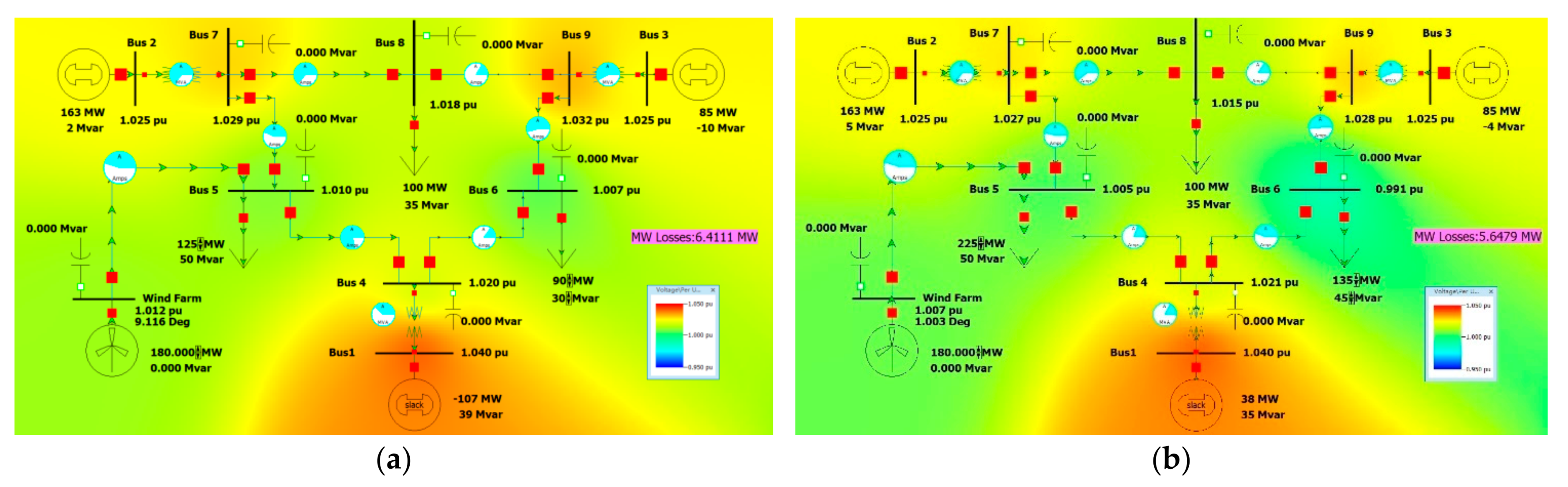
4.1. Bus 5 (25 km)

(1)

Simulation of tower A connected to bus 5

When tower A is used to connect 5 bus (25 km), the unit values of resistance, reactance, and susceptance of the long line are R = 0.001165, X = 0.011512, and B = 0.06144, respectively. I built the simulation model in PowerWorld as shown in Figure 1.

When operating under the minimum load, i.e., load 5–125 MW, 50 MVar, load 6–90 MW, 30 MVar, the system operation is shown in Figure 1a. It can be seen that the voltage of each bus is between 0.95–1.05 pu, and the line is not overloaded. The active network loss of the system is 6.4111 MW.

When operating under the maximum load, i.e., load 5–225 MW, 50 MVar, load 6–135 MW, 45 MVar, the system operation is shown in Figure 1b. It can be seen that the voltage of each bus is between 0.95–1.05 pu, and the line is not overloaded. The active network loss of the system is 5.6479 MW.

(2)

Simulation of tower B connected to bus 5

When B tower is used to connect 5 bus (25 km), the resistance, reactance, and susceptance of single-line unit value parameters are R = 0.001165, X = 0.011794, and B = 0.05992. The simulation model established in PowerWorld is shown in Figure 2.

When operating under the minimum load, i.e., load 5–125 MW, 50 MVar, load 6–90 MW, 30 MVar, the system operation is shown in Figure 2a. It can be seen that the voltage of each bus is between 0.95–1.05 pu, and the line is not overloaded. The active power loss of the system is 6.4131 MW.

When operating under the maximum load, i.e., load 5–225 MW, 50 MVar, load 6–135 MW, 45 MVar, the system operation is shown in Figure 2b. It can be seen that the voltage of each bus is between 0.95–1.05 pu, and the line is not overloaded. The active power loss of the system is 5.6498 MW.

(3)

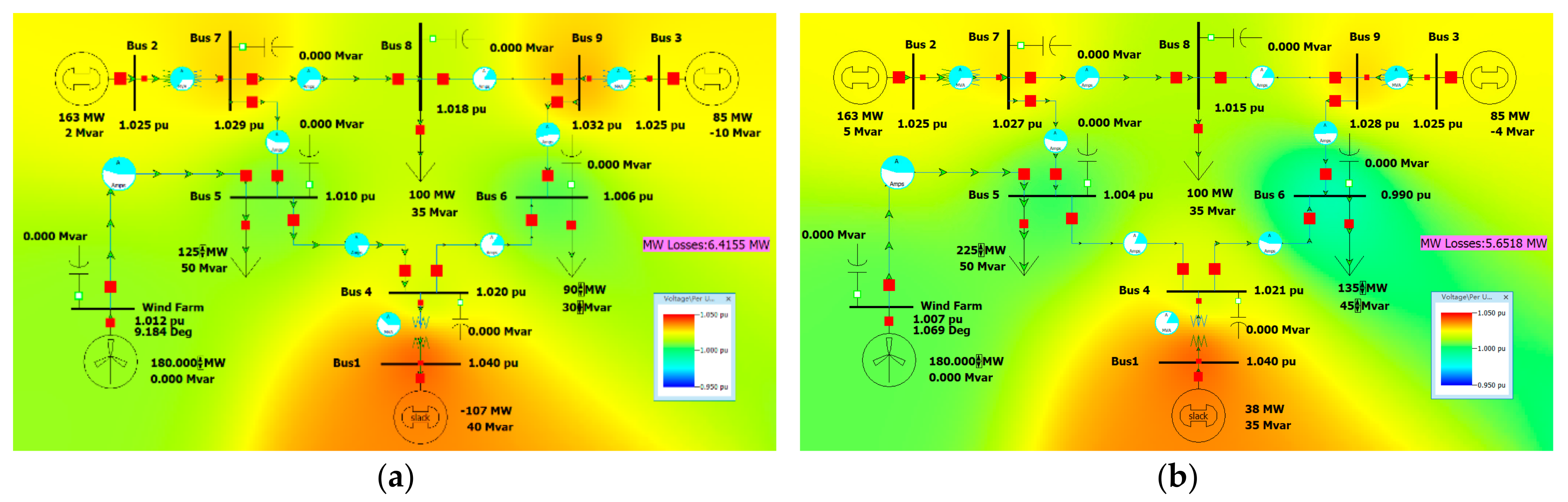
Simulation of tower C connected to bus 5

When Tower C is adopted and connected to Bus 5 (25 km), the resistance, reactance, and susceptance per unit value parameters of the long line are R = 0.001165, X = 0.012125, and B = 0.05823. The simulation model established in PowerWorld is as Figure 3.

When operating under the minimum load, i.e., load 5–125 MW, 50 MVar, load 6–90 MW, 30 MVar, the system operation is shown in Figure 3a. It can be seen that the voltage of each bus is between 0.95–1.05 pu, and the line is not overloaded. The active network loss of the system is 6.4154 MW.

When operating under the maximum load, i.e., load 5–225 MW, 50 MVar, load 6–135 MW, 45 MVar, the system operation is shown in Figure 3b. It can be seen that the voltage of each bus is between 0.95–1.05 pu, and the line is not overloaded. The active power loss of the system is 5.6518 MW.

4.2. Bus 6 (300 km)

(1)

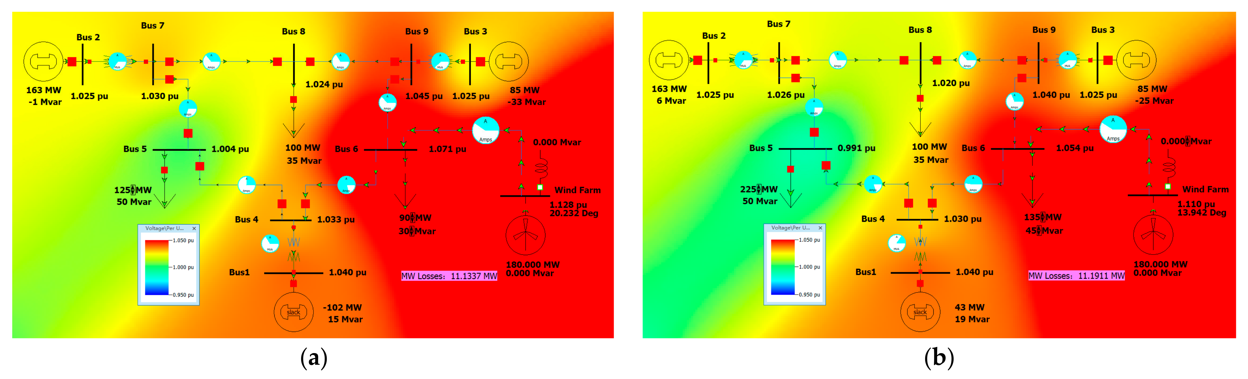
Simulation of tower A connected to bus 6

When Tower A is adopted and connected to Bus 6 (300 km), the resistance, reactance, and susceptance per unit value parameters RXGB of the line are 0.013508, 0.135835, 0.000646, and 0.743625. The simulation model established in PowerWorld is as follows.

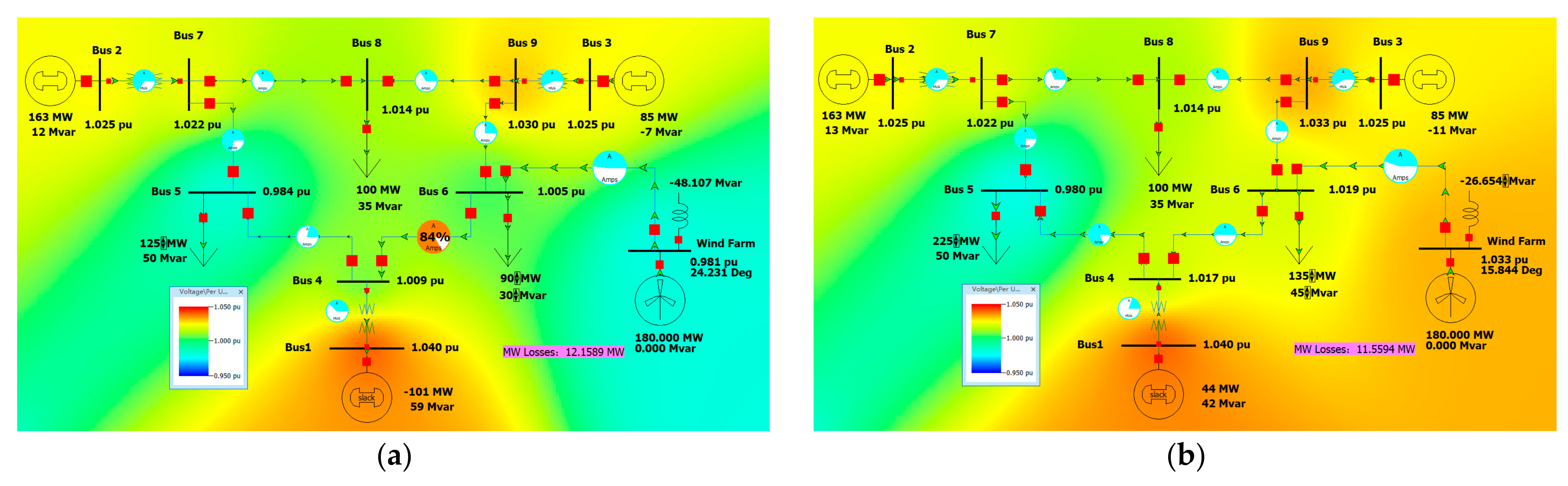
When operating under the minimum load, i.e., load 5–125 MW, 50 MVar, load 6–90 MW, 30 MVar, the system operation is shown in Figure 4. It can be seen that Bus 6 voltage exceeds 1.05 pu, and the lines are not overloaded. The active network loss of the system is 11.1137 MW.

To prevent the voltage from exceeding the range, I added an inductor with a rated capacity of 50 MVar to the outgoing bus of the wind farm. The voltage is within the normal range. The active power loss of the system is 12.1589 MW, as shown in Figure 5.

(2)

Simulation of tower B connected to bus 6

When Tower B is adopted and connected to Bus 6 (300 km), the resistance, reactance, and susceptance per unit value parameters RXGB of the line are 0.013508, 0.1391743, 0.000615, and 0.725225. The simulation model established in PowerWorld is as follows.

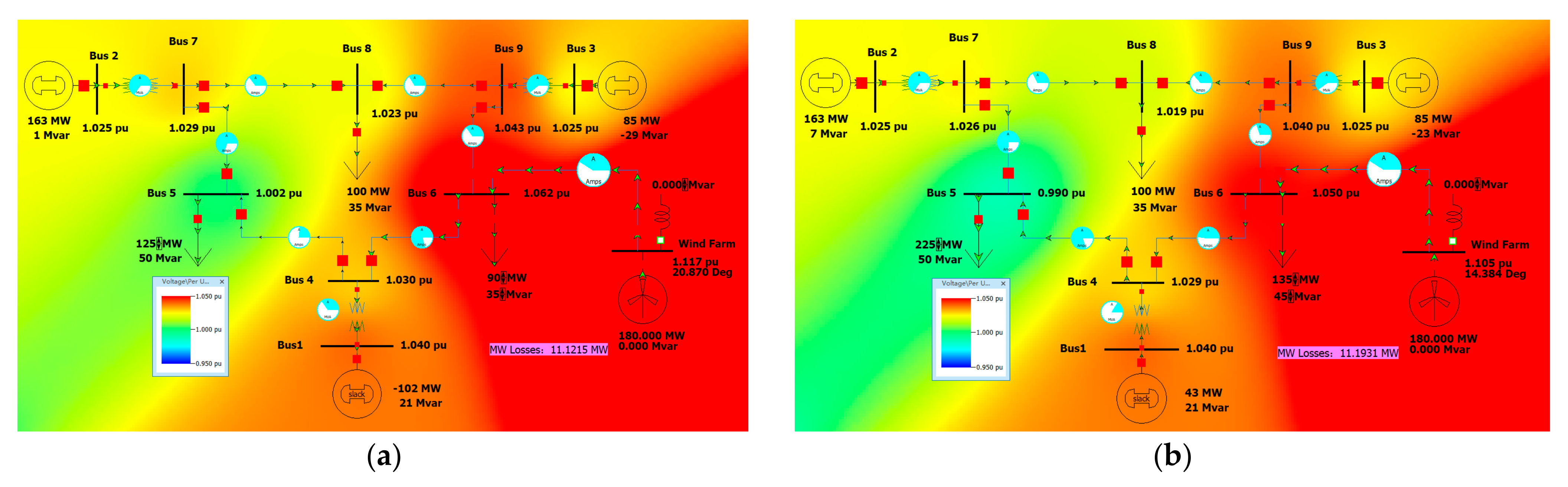
When operating under the minimum load, i.e., load 5–125 MW, 50 MVar, load 6–90 MW, 30 MVar, the system operation is shown in Figure 6a. It can be seen that the voltage of Bus 6 and Wind Farm bus exceeds 1.05 pu, and the lines are not overloaded. The active network loss of the system is 11.1215 MW.

When operating under the maximum load, i.e., load 5–225 MW, 50 MVar, load 6–135 MW, 45 MVar, the system operation is shown in Figure 6b. It can be seen that the bus voltage connected to the Wind Farm exceeds 1.05 pu, and the lines are not overloaded. The active network loss of the system is 11.1931 MW.

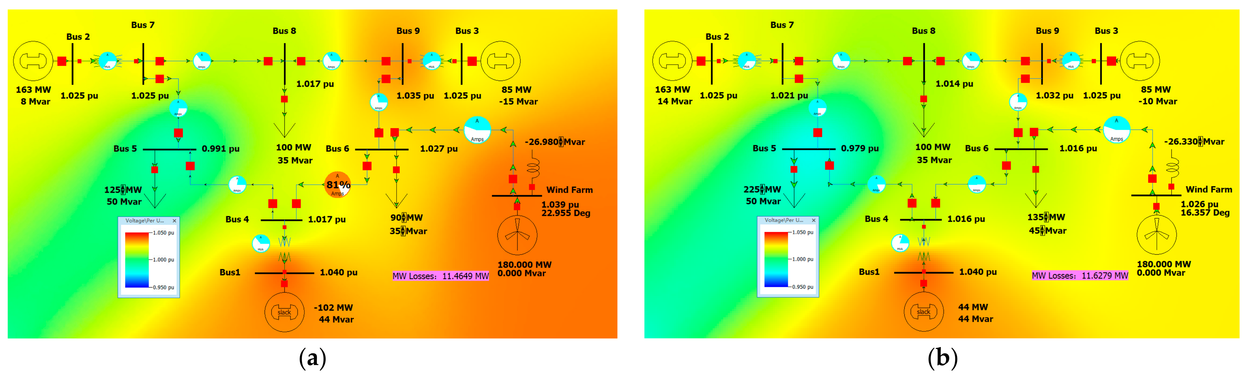
After an inductance with a rated capacity of 25 MVar is added to the outlet bus of the Wind Farm, the voltage is within the normal range. The active power loss of the system is 11.4649 MW as shown in Figure 7a.

After an inductance with a rated capacity of 25 MVar is added to the outlet bus of the Wind Farm, the voltage is within the normal range. The active power loss of the system is 11.6279 MW as shown in Figure 7b.

(3)

Simulation of tower C connected to bus 6

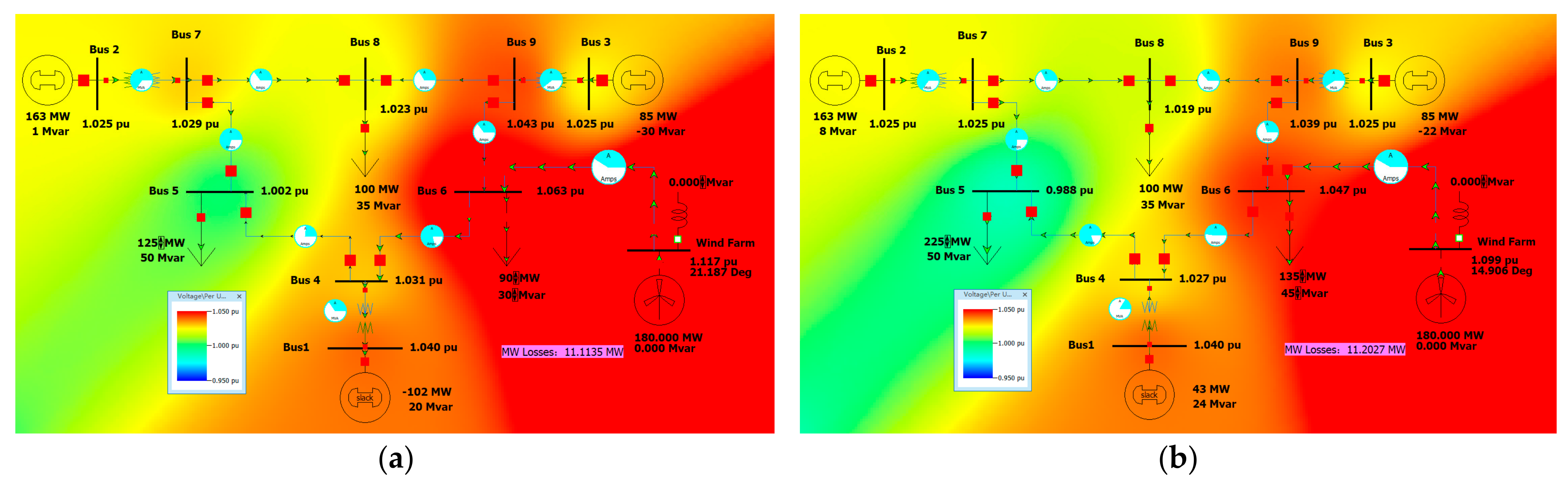
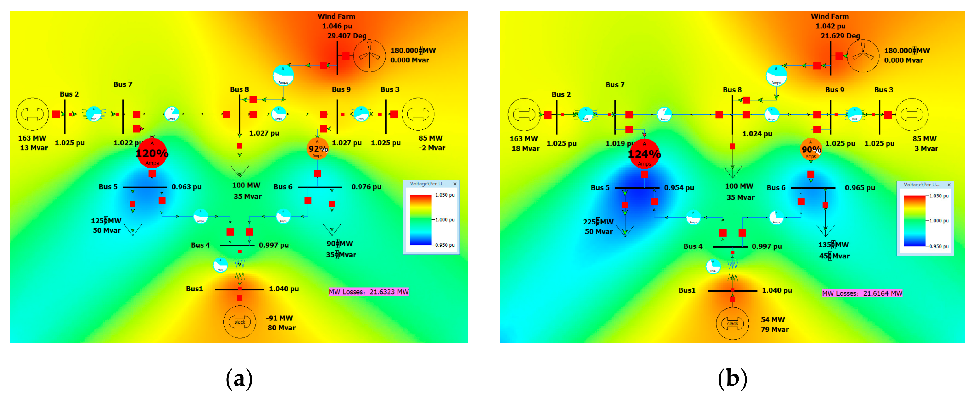
When Tower C is adopted and connected to Bus 6 (300 km), the resistance, reactance, and susceptance per unit value parameters RXGB of the line are 0.013509, 0.143086, 0.000581, and 0.704755. The simulation model established in PowerWorld is as follows.

When operating under the minimum load, i.e., load 5–125 MW, 50 MVar, load 6–90 MW, 30 MVar, the system operation is shown in Figure 8a. It can be seen that the voltage of Bus 6 and Wind Farm bus exceeds 1.05 pu, and the lines are not overloaded. The active network loss of the system is 11.1135 MW.

When operating under the maximum load, i.e., load 5–225 MW, 50 MVar, load 6–135 MW, 45 MVar, the system operation is shown in Figure 8b. It can be seen that the bus voltage connected to the Wind Farm exceeds 1.05 pu, and the lines are not overloaded. The active network loss of the system is 11.2027 MW.

After an inductance with a rated capacity of 25 MVar is added to the outlet bus of the Wind Farm, the voltage is within the normal range. The active power loss of the system is 11.4595 MW as shown in Figure 9a.

After an inductance with a rated capacity of 25 MVar is added to the outlet bus of the Wind Farm, the voltage is within the normal range. The active power loss of the system is 11.7152 MW as shown in Figure 9b.

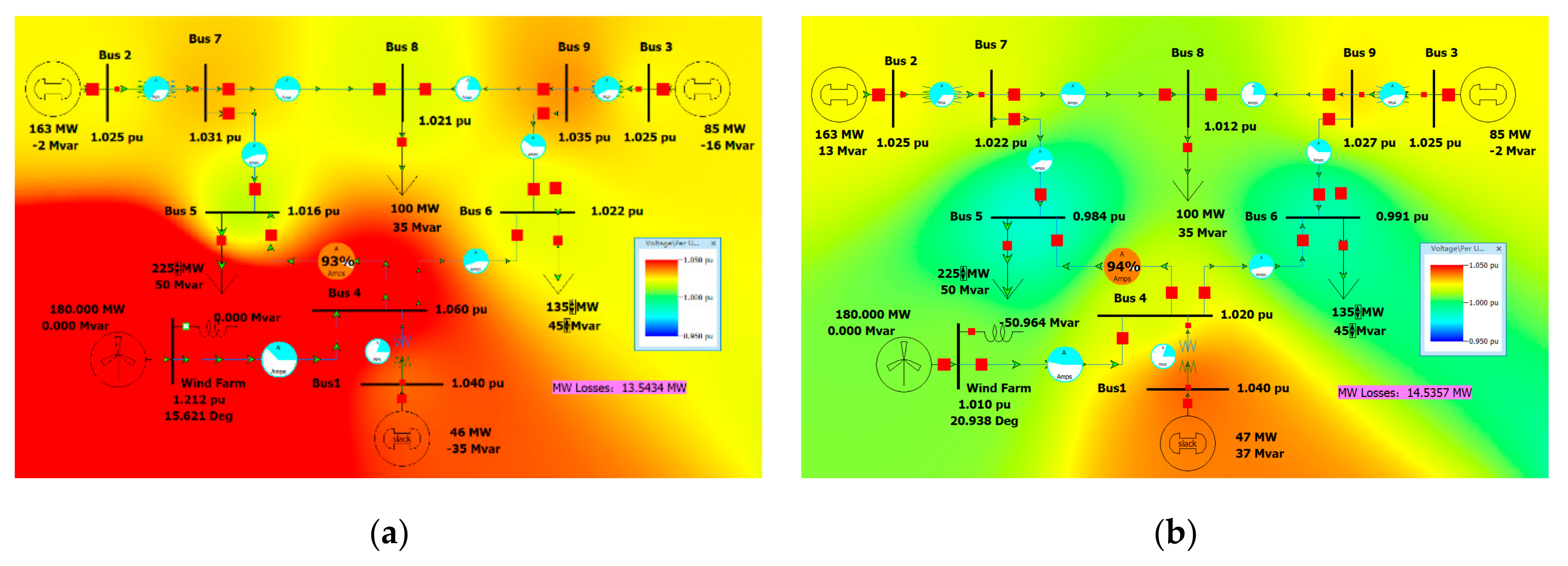
4.3. Bus 8 (150 km)

(1)

Simulation of tower A connected to bus 8

When Tower A is adopted and connected to Bus 8 (150 km), the resistance, reactance, and susceptance per unit value parameter RXGB of the line are 0.00693, 0.06878, 0.00008, and 0.369435. The simulation model established in PowerWorld is as follows.

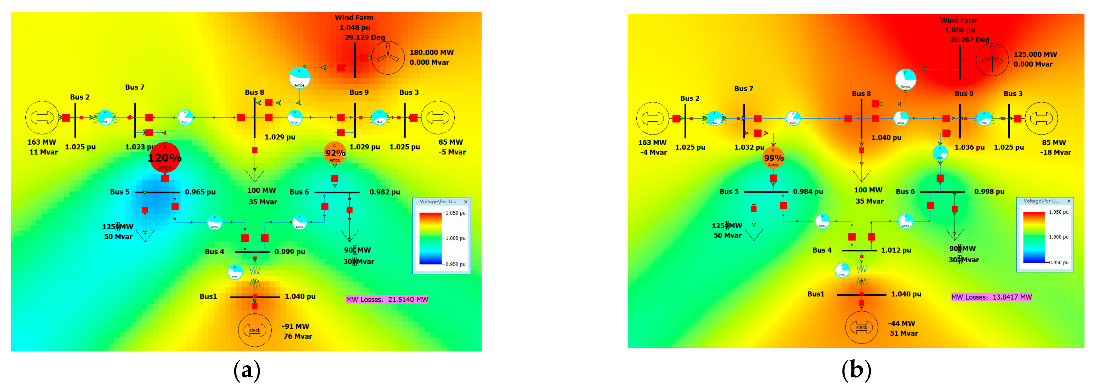
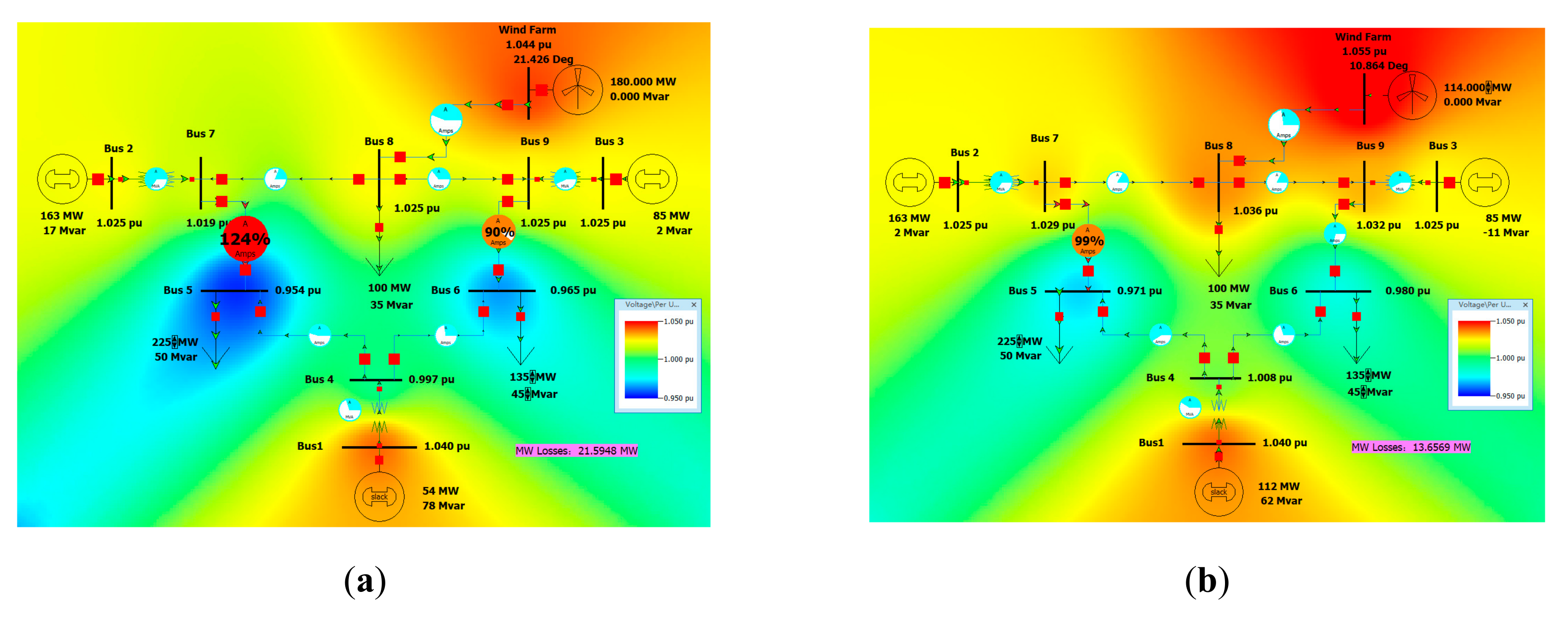
When operating under the minimum load, i.e., load 5–125 MW, 50 MVar, load 6–90 MW, 30 MVar, the system operation is shown in Figure 10a. Although the bus voltage is in the range of 0.95–1.05 pu, the power flow on Bus 7-8 and Bus 7-5 is changed due to the feeding of 180 MW power into Bus 8, and the line of Bus 7-5 is overloaded with a load rate of 120%. The active power loss of the system is 21.5140 MW. When the output of the Wind Farm is reduced to 125 MW, the Bus 7-5 line will not exceed the limit as shown in Figure 10b.

When operating under the maximum load, i.e., load 5–225 MW, 50 MVar, load 6–135 MW, 45 MVar, the system operation is shown in Figure 11a. The line load rate of Bus 7-5 still exceeds 100%. When the output of the Wind Farm is reduced to 114 MW, the line of Bus 7-5 does not exceed the limit, as shown in Figure 11b.

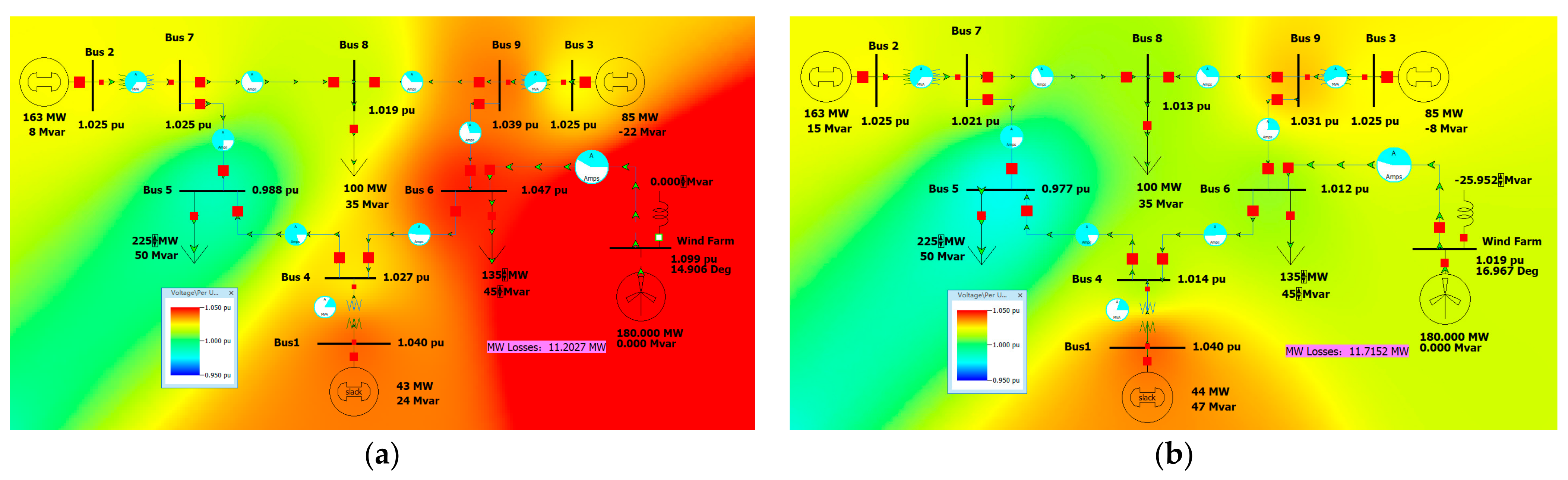
(2)

Simulation of tower B connected to bus 8

When Tower B is adopted and connected to Bus 8 (150 km), the resistance, reactance, and susceptance per unit value parameters RXGB of the long line are 0.00693, 0.0704732, 0.000076, and 0.360296.

When operating under the minimum load, i.e., load 5–125 MW, 50 MVar, load 6–90 MW, 30 MVar, the system operation is shown in Figure 12a. Although the bus voltage is in the range of 0.95–1.05 pu, the power flow on Bus 7-8 and Bus 7-5 is changed due to the feeding of 180 MW power into Bus 8, and the line of Bus 7-5 is overloaded with a load rate of 120%. The active power loss of the system is 21.5451 MW. When operating under the maximum load, i.e., load 5–225 MW, 50 MVar, load 6–135 MW, 45 MVar, the system operation is shown in the figure below. The line load rate of Bus 7-5 still exceeds 100%, as shown in Figure 12b. It is necessary to reduce the output of the Wind Farm so that the line is not overloaded.

(3)

Simulation of tower C connected to bus 8

When Tower C is adopted and connected to Bus 8 (150 km), the situation is the same as that of Tower A or B, and the line of Bus 7-5 is overloaded.

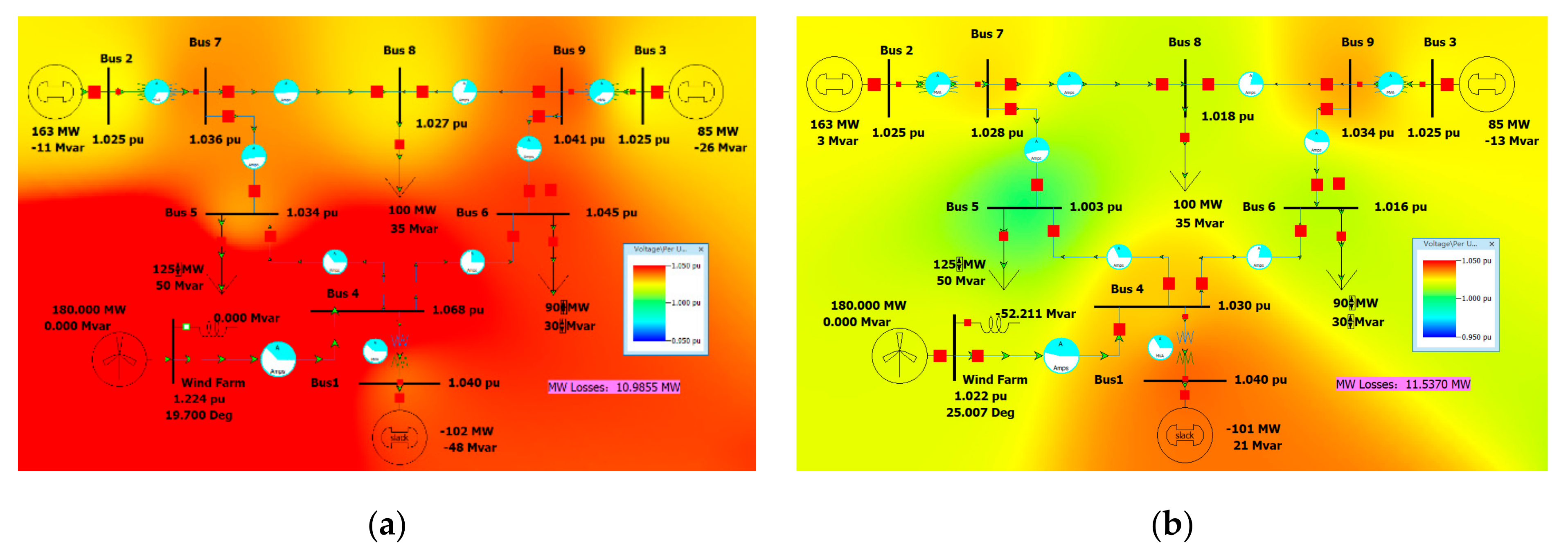
4.4. Bus 4 (500 km)

(1)

Simulation of tower A connected to bus 4

When Tower A is adopted and connected to Bus 4 (500 km), the resistance, reactance, and susceptance per unit value parameters RXGB of the long line are 0.0211477, 0.219643, 0.0031052, and 1.258646. The simulation model is established in PowerWorld, as shown in Figure 13.

When operating under the minimum load, i.e., load 5–125 MW, 50 MVar, load 6–90 MW, 30 MVar, the system operation is shown in Figure 13a. The voltage of Bus 4 and Wind Farm bus exceeds 1.05 pu. The active power loss of the system is 10.9855 MW. Add at least a reactor with a rated capacity of 50 MVar on the Wind Farm bus, and the bus voltage is restored to 0.95–1.05 pu. The system operation is as follows, and the system active power network loss is 11.5370 MW as shown in Figure 13b.

When operating under the maximum load, i.e., load 5–225 MW, 50 MVar, load 6–135 MW, 45 MVar, the system operation is shown in Figure 14a. The voltage of Bus 4 and Wind Farm bus exceeds 1.05 pu. Add at least a reactor with a rated capacity of 50 MVar on the Wind Farm bus, and the bus voltage is restored to 0.95–1.05 pu. The system operation is shown in Figure 14b, and the system active network loss is 14.5357 MW.

(2)

Simulation of tower B connected to bus 4

When Tower B is adopted and connected to Bus 4 (500 km), the resistance, reactance, and susceptance per unit value parameters RXGB of the line are 0.0211494, 0.2250446, 0.002953, and 1.227488. The system operation is the same as that when Tower A is used. Under the maximum or minimum load, the bus voltage of Bus 4 and Wind Farm exceeds 1.05 pu. Add a reactor with a rated capacity of 50 MVar at least on the Wind Farm bus, and the bus voltage is restored to 0.95–1.05 pu.

(3)

Simulation of tower C connected to bus 4

When Tower C is adopted and Bus 4 (500 km) is connected, the resistance, reactance, and susceptance per unit value parameters RXGB of the long line are 0.0211513, 0.2313719, 0.002788, and 1.192825. The system operation is the same as that when Tower A is used. Under the maximum or minimum load, the bus voltage of Bus 4 and Wind Farm exceeds 1.05 pu. Add a reactor with a rated capacity of 50 MVar at least on the Wind Farm bus, and the bus voltage is restored to 0.95–1.05 pu.

5. Results

According to the research and analysis of the above 12 cases, the connection of the wind power plant to Bus 8 will lead to the overload of lines 7-5, and thus the connection of Bus 8 is not considered. According to the need for capacitor reactor and system active power loss, nine other schemes meeting the constraints are listed in

Table 8. Comparison of different access bus schemes.

Scheme Number	Tower	Bus	Reactor (Each Cost 25 MVar)	Losses in Minimum Load Condition (MW)	Losses in Maximum Load Condition (MW)
1	A	Bus 5	0	6.4111	5.6479
2	B	Bus 5	0	6.4131	5.6498
3	C	Bus 5	0	6.4154	5.6518
4	A	Bus 6	1	12.1589	11.5594
5	B	Bus 6	1	11.4649	11.6279
6	C	Bus 6	1	11.4595	11.7152
10	A	Bus 4	2	11.5370	14.5357
11	B	Bus 4	2	11.6687	14.7109
12	C	Bus 4	2	11.8451	14.9421

.

When Tower A is adopted, the active power loss of the system is slightly smaller than that when Tower B and C are adopted, and the construction cost of Tower A is also the least.

Selecting Bus 5 to connect to the Wind Farm has less network loss than Bus 6 and Bus 4. At the same time, it can meet the voltage of each bus between 0.95–1.05 pu without a reactor. Since Bus 5 is closest to the Wind Farm (25 km), the material cost and construction cost will be lower than Bus 6 (300 km) and Bus 4 (500 km). Therefore, it is more appropriate to connect Bus 5.

The material cost of Tower A is $62,000 per km. If Bus 5 is 25 km away from the Wind Farm, the material cost of the tower is $1,550,000. The material cost of two AAC 31.5 mm diameter is $32,600 per km.

The construction cost of two bundle conductors is $35,000 per km, and thus the total cost per unit length of conductor is $67,600 per km. The total cost of a 25 km conductor is $1,690,000; therefore, the total cost of a 25 km tower and conductor is $3,240,000.

Similarly, calculate the line erected by Tower B and Tower C and select Bus 5 (25 km) for access. The cost of a single conductor of AAC 31.5 mm diameter is $16,300 per km, and the construction cost of two split conductors is $35,000 per km. I calculate the total costs and list them in

Table 9. Cost comparison of different towers.

Scheme Number	Tower	Tower Cost $ per km	Total Cost $
1	A	62,000	3,240,000
2	B	74,000	3,540,000
3	C	76,000	3,590,000

. It can be seen that option 1 selects tower type A with the lowest cost.

In conclusion, it is a reasonable choice to select Tower A, with Bus 5 connected to the Wind Farm.

I perform a power flow analysis on the best combination, testing the data with and without the wind farm connected to the system. When the Wind Farm is connected to the system through Bus 5, under the maximum load, the bus voltage is between 0.95–1.05 pu, the lines are not overloaded, and the system active network loss is 5.6480 MW. Under the minimum load, the bus voltage is between 0.95–1.05 pu, the lines are not overloaded, and the system active network loss is 6.4110 MW.

When the Wind Farm is not connected to the system, the bus voltage is between 0.95–1.05 pu, the lines are not overloaded, and the system active network loss is 7.5720 MW. Under the minimum load, when the Wind Farm is not connected to the system, the bus voltage is between 0.95–1.05 pu, the lines are not overloaded, and the system active network loss is 4.6275 MW. All data are within safe limits.

6. Discussion

Enhancing the coordination between wind power and electric vehicles is helpful for promoting the maximum utilization of wind power and improving the economic benefits of the converter stations. At the same time, the reform of the national power industry has also provided a huge boost to the cooperation between the two, thus, achieving the effect of “1 + 1 > 2” and promoting a win–win situation for the industrial chain. Therefore, the study of the synergistic effect of wind power generation and electric vehicle converter stations has important theoretical significance as well as practical concerns regarding alleviation of the dual pressure of the energy crisis and environmental pollution, promotion of the development and utilization of wind power generation, and promotion of the rapid development of the electric vehicle industry.

Due to the randomness and uncertainty of wind speed and the influence of the tower shadow effect and wind shear, vibration always accompanies the operation of these units. The vibration of the unit will not only produce huge pollution noise but also cause the loosening of the parts of the unit and damage of the actuator, which seriously affects the service life of the unit. The vibration mainly involves transmission chain torsional vibration, tower cylinder vibration, blade flutter, and a possible coupling vibration among them.

The torsional vibration of the transmission chain can cause not only the damage of gearbox and coupling but also sub-synchronous oscillation and sub-synchronous harmonics. All of these will reduce the security of the power supply and bring higher hidden costs. These aspects are not considered in this study. In future studies, if the vibration of wind turbines can be taken into account, this scheme will be improved.