Research on Charging-Discharging Operation Strategy for Electric Vehicles Based on Different Trip Patterns for Various City Types in China

Abstract

Connecting large numbers of electric vehicles to the power grid creates challenges for the operation of the power distribution network, but also provides a new method for supporting grid operation. This paper considers the trip patterns of electric vehicle users in China, including their trip starting time, traffic congestion, vehicle energy consumption, and other factors. We develop a charging–discharging operation strategy for electric vehicles in different functional areas with the goal of minimizing the cost of distribution network, which considers the distribution patterns of electric vehicles in different functional areas. As different types of cities in China have different proportions of electric vehicle users who follow different travel chains, we provide multiple examples showing the effectiveness of our proposed V2G method in different cities.

1. Introduction

To reduce fossil fuel consumption and the emission of greenhouse gases, including carbon dioxide and other harmful gases, governments of all countries have promoted electric vehicles (EV) as a substitute for traditional fossil fuel vehicles. On one hand, given the unpredictable charging behavior of EV users, connecting many EV charging loads to the power grid may create problems by increasing peak load and causing power grid voltage fluctuations. Appropriate charging strategies should therefore be adopted to minimize the adverse impact of EVs on the power grid. On the other hand, EV batteries serve as a kind of mobile energy storage. They can participate in the demand response by coordinating their charging and discharging strategies to promote economy in power grid operation, and the development of vehicle-to-grid (V2G) technology can further support power grid operation [1,2,3,4].

Previous studies predicted the distribution, travel time, and mileage of EVs and optimized EV charging based on this distribution rule [5,6,7]. However, these studies did not consider the transfer of EVs in different spaces or its spatial distribution. Zhou et al. [8] proposed an EV charging strategy that was based on information about user travel chains and traffic networks and considered the travel time of electric vehicles; the authors additionally derived a model predicting the temporal and spatial distribution of EV load under this strategy. Moghaddass et al. [9] similarly used a mixed integer multi-objective optimization model to optimize an EV charging strategy that accounted for the power supply cost of the grid, load fluctuation, EV charging station benefits, user charging costs, and household electricity patterns. Other studies have proposed different control strategies by considering the possibility of EV battery discharge and studying V2G strategies [10,11,12]. These studies scheduled charging and discharging times for each vehicle and verified the feasibility of their scheduling strategy in real-world situations.

The studies mentioned above all determined the temporal and spatial distribution of EVs using the Monte Carlo simulation method. However, as the number of EVs in the current city increases, the calculation time required for traditional Monte Carlo sampling gradually increases. As cluster EVs will gradually become uniformly distributed as the number of EVs increases, the probability distribution formula can mathematically derived.

In this study, we develop a charging–discharging operation strategy for electric vehicles based on different trip patterns for various city types with the intention of minimizing the cost of distribution network. Firstly, we determine the probability distribution formula of EVs based on the travel patterns of EV users while also considering trip rules of Chinese residents and traffic congestion. In addition, because different EV users have different travel patterns, the spatiotemporal distribution of EVs differs among functional areas. We also consider the distribution network power flow and voltage constraints based on the second-order cone relaxation method, and we analyze the charging and discharging strategy of cluster EVs for different EV distribution patterns in different functional areas. Finally, based on the proportion of EV users following each defined travel pattern, we obtained the EV distribution patterns for different types of cities in China, as well as the charging and discharging strategies, distribution network costs, and EV user profits in these cities.

This paper is organized as follows. In Section 2, the time and space distribution models of EVs are established based on different travel patterns of EVs in China. In Section 3, the charging and discharging model of aggregated EVs is designed, and the electric vehicle scheduling model is established in Section 4 considering the distribution network power flow and voltage constraints. Algorithm flow chart is demonstrated in Section 5. The profitability of our strategy is verified in Section 6. Section 7 summarizes the findings of paper.

2. Time and Space Distribution Model of Electric Vehicles

2.1. Electric Vehicle Travel Chain

EVs can be categorized according to the type of travel they are used for (e.g., private cars for work purposes, private cars for non-work purposes, official cars for corporate travel, etc.). Here, we focus on private cars used for work or entertainment and fully consider people’s life habits when simulating user trip patterns. We also adopt a “travel chain” structure to represent the travel time, travel destination, and trip itinerary of EV users and the sequence of each trip [13]. Overall, the travel of an EV used for work and entertainment can be roughly divided into trips to/from home, work, and entertainment, which we represent using the English letters H, W, and E, respectively.

According to the literature [14], 98.21% of private car trips start and end at home. The number of daily trips taken by urban residents ranges from 2 to 3.5; this number decreases from small cities to big cities and increases from economically underdeveloped cities to developed cities [15,16,17]. 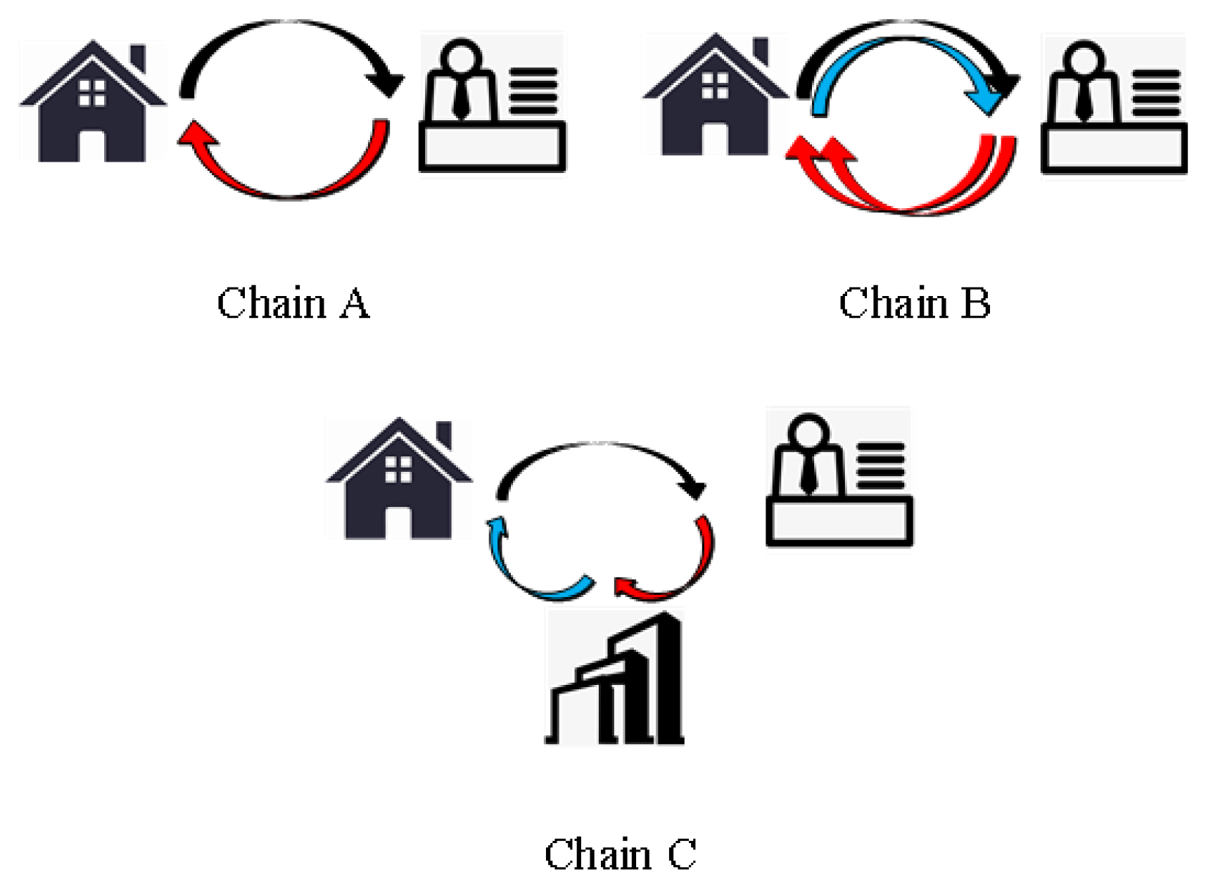As travel is convenient in small cities, residents of these cities often take an extra trip home for lunch at noon [18]. Entertainment options are more abundant for residents of large, economically developed cities, and these residents therefore travel for entertainment consumption in the evening. This paper considers three modes of travel chain structure: the simple work chain “A” (H–W–H), the complex work chain “B” (H–W–H–W–H), and the work–entertainment chain “C” (H–W–E–H).

2.2. Distribution Network Function Division

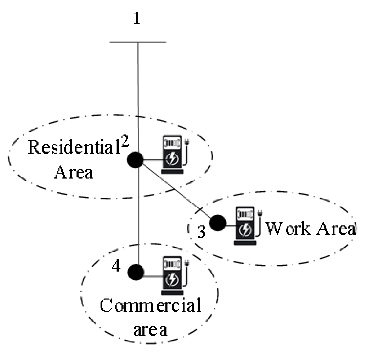
Any geographical area can be functionally subdivided depending on the purpose of the trip to that area (residential areas, working areas, and commercial areas, etc.). Given the distribution network topology over the whole region, each subordinate node of the distribution network area can be geographically allocated to various functional areas. For example, in a four-node distribution network, each grid node (except for the root node) will be divided into corresponding functional areas and equipped with EV charging stations, as shown in Figure 1. In one day, EVs drive between each functional area according to the travel chain they are following (defined above). If the functional area has multiple nodes that are equipped with EV charging stations, we assume that EVs are evenly distributed among each node that is equipped with charging stations. The average distance between each region is selected in the calculation, and Lij (i,j ∈ [1, 3]) is the distance between each region.

2.3. Distribution of Electric Vehicles in Each Functional Area at Each Time Period

At any given time, the distribution of subordinate nodes of EVs in each functional area is related to the departure and arrival conditions of EVs under each trip. These conditions can be expressed using their corresponding probability distribution functions. As shown in Figure 2, the probability distribution functions for departures and arrivals of similar trips from each travel chain structure can adopt the same form. Trips from each travel chain can therefore be divided into three categories based on the probability distribution function they follow:

• Type 1 (black line in Figure 2) refers to the working trip, including the H–W trip of the simple work chain A, the first H–W trip of the complex work chain B, and the H–W trip of the work–entertainment chain C.
• Type 2 (red line in Figure 2) mainly includes home or entertainment trips, including the W–H trip of the simple work chain A, both W–H trips of the complex work chain B, and the W–E trip of the work–entertainment chain C.
• Type 3 (blue line in Figure 2) includes the second H–W trip of the complex work chain B and the E–H trip of the work–entertainment chain C.

2.3.1. Type 1 Trips

Trip type 1 mainly includes the first trip to the working area: the H–W trip in the simple work chain A, the first H–W trip in the complex work chain B, and the H–W trip in the work–entertainment chain C. Travel time for these trips follows a normal distribution [15,19]. The mean and standard deviation of the travel time for different users can vary, but they can be fitted with a certain distribution function. For trip type 1, the mean user departure time conforms to a gamma distribution, and the standard deviation conforms to a standard normal distribution [8,16]. Based on these distributions of the means and standard deviations, we solved the edge probability distribution of variable T to obtain the probability density formula (1) and cumulative distribution function (2) for the departure time of trip type 1. See Appendix A for details.

$$f_1^{\mathrm{lv}}(t)={\displaystyle \underset{0}{\overset{\infty }{\int }}{\displaystyle \underset{0}{\overset{\infty }{\int }}\frac{2{\theta }^{-\alpha }{\mu }^{\alpha -1}}{\sigma {\sigma }_2\pi \cdot \mathrm{\Gamma }(\alpha )}\cdot \exp \left(-\frac{{(t-\mu )}^2}{2{\sigma }^2}-\frac{\mu }{\theta }-\frac{{\sigma }^2}{2{\sigma }_2{}^2}\right)}}d\mu d\sigma$$

(1)

$$F_1^{\mathrm{lv}}(t)={\displaystyle \underset{0}{\overset{t}{\int }}{f}_1^{\mathrm{lv}}(\tau )d\tau }$$

(2)

In these equations, t is the start time of EV travel, μ is the mean EV start time, σ is the standard deviation of the EV start time, α and θ are the scale and shape parameters of the gamma distribution, respectively, and σ₂ is the standard deviation of the standard normal distribution.

The gamma distribution and the parameters for the standard normal distribution are shown in Appendix A for the different trip types. Using these distributions, we can obtain the probability density function and cumulative distribution function for the H–W trip in simple work chain A, the first H–W trip in the complex work chain B, and the H–W trip in the work–entertainment chain C.

As the cumulative distribution function of arrival time is related to the travel time between home and work, this function can be obtained by combining the cumulative distribution functions of departure times and travel times. If traffic congestion is considered during travel, the congestion coefficient can be set based on the time of day, as shown in

Table 1. Congestion coefficient at different times of day.

Time	Morning Peak 7:00–9:00	Evening Peak 17:00–19:00	Other Time 0:00–7:00, 9:00–17:00, 19:00–24:00
Congestion coefficient	1.5	1.5	1

. Vehicle speed during the congestion period is divided by the congestion coefficient.

If the start time of congestion is $t_{\mathrm{s}}^{\mathrm{jam}}$, the end time of congestion is $t_{\mathrm{end}}^{\mathrm{jam}}$, and the congestion parameter ε = 1.5, then the total journey time is:

$$\mathrm{\Delta }{t}_{ij,t}=\{\begin{array}{ll}\frac{L_{ij}}{v}& t_{i,j}^{\mathrm{arr}}\le t_{\mathrm{s}}^{\mathrm{jam}}\hfill \\ \frac{L_{ij}}{v}+(1-\frac{1}{\mathsf{\epsilon }})(t_{i,j}^{\mathrm{arr}}-t_{\mathrm{s}}^{\mathrm{jam}})& t_{\mathrm{s}}^{\mathrm{jam}}<t_{i,j}^{\mathrm{arr}}\le t_{\mathrm{s}}^{\mathrm{jam}}+\frac{\mathsf{\epsilon }{L}_{ij}}{v}\hfill \\ \frac{\mathsf{\epsilon }{L}_{ij}}{v}& t_{\mathrm{s}}^{\mathrm{jam}}+\frac{\mathsf{\epsilon }{L}_{ij}}{v}<t_{i,j}^{\mathrm{arr}}\le t_{\mathrm{end}}^{\mathrm{jam}}\hfill \\ \frac{\mathsf{\epsilon }{L}_{ij}}{v}-(\mathsf{\epsilon }-1)(t_{i,j}^{\mathrm{arr}}-t_{\mathrm{end}}^{\mathrm{jam}})& t_{\mathrm{end}}^{\mathrm{jam}}<t_{i,j}^{\mathrm{arr}}\le t_{\mathrm{end}}^{\mathrm{jam}}+\frac{L_{ij}}{v}\hfill \\ \frac{L_{ij}}{v}& t_{i,j}^{\mathrm{arr}}>t_{\mathrm{end}}^{\mathrm{jam}}+\frac{L_{ij}}{v}\hfill \end{array}$$

(3)

where Δt_ij,t indicates the travel time of the electric vehicle for a trip from region i to region j, arriving at time t. v indicates the speed of the electric vehicle, and $t_{i,j}^{\mathrm{arr}}$ indicates the arrival time for the journey from region i to region j.

The cumulative distribution function for the arrival time is:

$$F_1^{\mathrm{arr}}(t)=F_1^{\mathrm{lv}}(t-\mathrm{\Delta }{t}_{12,t})$$

(4)

2.3.2. Type 2 Trips

Trip type 2 mainly consists of trips to home or entertainment: the W–H trip in simple work chain A, both W–H trips in complex work chain B, and the W–E trip in work-entertainment chain C. The departure time for these trips follows a normal distribution. The Weibull and normal distributions were used to fit the mean and standard deviations, respectively, for different EV users [20]. We then obtained the corresponding probability density formula (5) and cumulative distribution function formula (6); the detailed derivation process is shown in Appendix B.

$$f_2^{\mathrm{lv}}(t)={\displaystyle \iint \{\frac{k}{2\mathsf{\pi }\sigma {\sigma }_3\lambda }\cdot {\left(\frac{\mu }{\lambda }\right)}^{k-1}}\cdot \exp \left(-\frac{{(t-\mu )}^2}{2{\sigma }^2}-{\left(\frac{\mu }{\lambda }\right)}^k-\frac{{(\sigma -{\mu }_2)}^2}{2{\sigma }_3^2}\right)\}d\mu d\sigma$$

(5)

$$F_2^{\mathrm{lv}}(t)={\displaystyle \underset{0}{\overset{t}{\int }}{f}_2^{\mathrm{lv}}(\tau )d\tau }$$

(6)

In these equations, μ is fitted by the Weibull distribution, and k and λ are the shape parameters and scale parameters, respectively, of the Weibull distribution. The standard deviation is fitted by the normal distribution, and μ₂ and σ₃ are the mean and standard deviation, respectively, of the normal distribution.

Parameters of the Weibull and normal distributions for the different type 2 trips are shown in Appendix B. Using these parameters, we can obtain the probability density and cumulative distribution functions of the W–H trip in simple work chain A, both W–H trips in complex work chain B, and the W–E trip in work–entertainment chain C.

Combined with the return journey time, the cumulative distribution function of the type 2 trips to residential or commercial areas is given by:

$$F_2^{\mathrm{arr}}(t)=F_2^{\mathrm{lv}}(t-\mathrm{\Delta }{t}_{2j,t}) j=1,3$$

(7)

2.3.3. Type 3 Trips

Trip type 3 includes the second H–W trip in the complex work chain B and the E–H trip in the work–entertainment chain C. As the departure time for the second H–W trip in small cities is related to the “stay” time at home for lunch, and the departure time for the E–H trip in big cities is related to the stay time in the commercial area, we assume the stay time follows a random distribution [8], which is expressed as Δt ~ U(Δt_min, Δt_max). I this equation, Δt_min is the shortest residence time and Δt_max is the longest residence time. The probability density function for the H–W departure time is given by Formula (8), and the cumulative distribution function is given by Formula (9):

$$\begin{array}{l}{f}_3^{\mathrm{lv}}(t)={\displaystyle {\int }_{t-\mathrm{\Delta }{t}_{\max }}^{t-\mathrm{\Delta }{t}_{\min }}{f}_{\mathrm{last}}^{\mathrm{arr}}(\tau )\cdot \frac{1}{\mathrm{\Delta }{t}_{\max }-\mathrm{\Delta }{t}_{\min }}d\tau }\\ \hspace{1em} =\frac{1}{\mathrm{\Delta }{t}_{\max }-\mathrm{\Delta }{t}_{\min }}(F_{\mathrm{last}}^{\mathrm{arr}}(t-\mathrm{\Delta }{t}_{\min })-F_{\mathrm{last}}^{\mathrm{arr}}(t-\mathrm{\Delta }{t}_{\max }))\end{array}$$

(8)

$$F_3^{\mathrm{lv}}(t)={\displaystyle \underset{0}{\overset{t}{\int }}{f}_3^{\mathrm{lv}}(\tau )d\tau }$$

(9)

$f_{\mathrm{last}}^{\mathrm{arr}}$(τ) is the probability density function of the arrival time of the last trip. The values of Δt_min and Δt_max for different trips are shown in Appendix C.

The formula of the cumulative distribution function for arriving at the working or residential area for type 3 trips, accounting for journey time, is shown in Formula (10):

$$F_3^{\mathrm{arr}}(t)=F_3^{\mathrm{lv}}(t-\mathrm{\Delta }{t}_{ij,t})$$

(10)

2.3.4. EV Departure, Arrival, and Distribution Probability in Each Region

The departure time distribution function of EVs in each space can be seen as the probability of EVs leaving the space at each time. Conversely, the arrival time distribution function of EVs can be regarded as the probability of EVs arriving in the space at each time. Therefore, the equations derived in Section 2.3.1 to Section 2.3.3 can be used to calculate the probability of leaving from and arriving in each region at each time, for each trip in each of the three travel chains, while accounting for the proportion of EVs using the different travel chains. For example, the probability of EVs leaving area 1 (a residential area) is:

$$f_{1,t}^{\mathrm{lv}}={\beta }_A{f}_{12}^{\mathrm{lv}\_\mathrm{A}}(t)+{\beta }_B{f}_{12}^{\mathrm{lv}\_\mathrm{B}}(t)+{\beta }_C{f}_{12}^{\mathrm{lv}\_\mathrm{C}}(t)$$

(11)

where β_A, β_B, and β_C are the proportions of EVs using travel chains A, B, and C, respectively, and $f_{12}^{\mathrm{lv}\_\mathrm{A}}$(t), $f_{12}^{\mathrm{lv}\_\mathrm{B}}$(t), and $f_{12}^{\mathrm{lv}\_\mathrm{C}}$(t) are the moment-by-moment probabilities of a user leaving area 1 for the trip from area 1 (residential area) to area 2 (working area) under travel chains A, B and C, respectively.

Similarly, the arrival and departure probabilities of EVs at time t in region I are $f_{i,t}^{\mathrm{lv}}$ and $f_{i,t}^{\mathrm{arr}}$, respectively. By subtracting the cumulative probability function of leaving each region from the cumulative probability function of arriving in the corresponding region, we can determine that the distribution probability of EVs at time t in region i is η_i,t.

3. Model for the Charging and Discharging of Electric Vehicles

3.1. Energy Consumption Model

Unlike energy storage, the state of charge (SOC) of the battery will decrease as EVs consume energy while driving. Here, we define the energy consumption factor as ψ. The energy consumption of each EV for travel from i to j (i ≠ j) is:

$$\mathrm{\Delta }{E}_{ij}=\psi \cdot L_{ij}$$

(12)

For this model, we assume that the travel chain of EV users in small cities includes the simple work chain A and the complex work chain B, and that the travel chain of EV users in large cities includes the simple work chain A and the work–entertainment chain C.

3.1.1. EV Energy Consumption Model at the Workspace Node

For trips starting from the residential area, the total energy consumed by all EVs arriving at a node in the working area at time t is:

$$\mathrm{\Delta }{E}_{2,t}=\left[N_{\mathrm{all}}\cdot f_2^{\mathrm{arr}}(t)\cdot \frac{1}{N_2}\right]\cdot \mathrm{\Delta }{E}_{12}$$

(13)

where N_all indicates the possession of EVs. N_i is the number of nodes with EV charging stations in region i, and [] is the round-up function.

3.1.2. EV Energy Consumption Model at the Commercial Node

For trips starting from the working area, the total energy consumed by all EVs arriving at a node in the commercial area at time t is:

$$\mathrm{\Delta }{E}_{3,t}=\left[N_{\mathrm{all}}\cdot f_3^{\mathrm{arr}}(t)\cdot \frac{1}{N_3}\right]\cdot \mathrm{\Delta }{E}_{23}$$

(14)

3.1.3. EV Energy Consumption Model at the Residential Node

For trips starting from the working or commercial areas, the total energy consumed by all electric cars arriving at a node in the residential area at time t is:

$$\mathrm{\Delta }{E}_{1,t}=\left[(f_1^{\mathrm{arr}}(t)-{\beta }_C\cdot f_{31}^{\mathrm{arr}}(t))\cdot \frac{N_{\mathrm{all}}}{N_1})\right]\cdot \mathrm{\Delta }{E}_{21}+\left[{\beta }_C{N}_{\mathrm{all}}\cdot f_{31}^{\mathrm{arr}}(t)\cdot \frac{1}{N_1}\right]\cdot \mathrm{\Delta }{E}_{31}$$

(15)

where $f_{31}^{\mathrm{arr}}$(t) indicates the probability that an EV reaches the residential area at time t in the E–H trip in travel chain C. In Formula (15), the first term represents the energy consumption of cluster EVs arriving in residential areas as part of travel chains A and B at each moment, and the second term represents the energy consumption of cluster EVs arriving in residential areas as part of travel chain C.

3.2. Charging and Discharging Model of Cluster Electric Vehicles

3.2.1. Charging and Discharging Constraints

The charging and discharging constraints at nodes in region i that are equipped with charging stations are as follows:

$$-\left[{\eta }_{i,t}{N}_{\mathrm{all}}\frac{1}{N_i}\right]P_{\max }^{\mathrm{D}}\le u_{k,t}\le \left[{\eta }_{i,t}{N}_{\mathrm{all}}\frac{1}{N_i}\right]P_{\max }^{\mathrm{C}}$$

(16)

where $P_{\max }^{\mathrm{D}}$ and $P_{\max }^{{C}}$ are the maximum discharge and charging power, respectively, of each vehicle, and u_k,t is the charging and discharging power of node k at time t. By convention, charging is positive and discharging is negative.

3.2.2. Capacity Constraint

We required the capacity Q_k,t of node k at time t to equal or exceed the SOC value required by the EVs leaving at time below and the sum of the minimum SOC values required by the remaining EVs, as shown in Formula (17). Conversely, Q_k,t could not exceed the maximum allowable SOC value of the node, as shown in Formula (18).

$$Q_{k,t}\ge \left[f_{i,t+1}^{\mathrm{lv}}{N}_{\mathrm{all}}\frac{1}{N_i}\right]{\gamma }_i^{\mathrm{lv}}C+\left[({\eta }_{i,t}-f_{i,t+1}^{\mathrm{lv}})N_{\mathrm{all}}\frac{1}{N_i}\right]{\gamma }^{\mathrm{dw}}C$$

(17)

$$Q_{k,t}\le \left[{\eta }_{i,t}{N}_{\mathrm{all}}\frac{1}{N_i}\right]{\gamma }^{\mathrm{up}}C$$

(18)

In these two equations, i is the region to which node k belongs, γ^dw indicates the minimum SOC requirement for each EV, ${\gamma }_i^{\mathrm{lv}}$ indicates the SOC required for each EV leaving area i, and C is the battery capacity of each EV.

3.2.3. Continuity Constraints on SOC

We defined the continuity constraints on SOC as:

$$Q_{k,t}=Q_{k,t-1}+\mathsf{\chi }{u}_{k,t-1}{\delta }_{\min }+\frac{1}{N_i}{N}_{\mathrm{all}}{f}_{i,t}^{\mathrm{arr}}{\gamma }_{i-1}^{\mathrm{lv}}C-\mathrm{\Delta }{E}_{i,t}-\frac{1}{N_k}{N}_{\mathrm{all}}{f}_{i,t}^{\mathrm{lv}}{\gamma }_k^{\mathrm{lv}}C$$

(19)

where χ indicates the charging and discharging efficiency of EVs and δ_min indicates the minimum time unit, which we set at 15 minutes for this study. Note that the last three terms of Formula (19) account for the quantity of electricity added by newly arriving EVs and the quantity of electricity taken away by newly departing EVs.

4. Electric Vehicle Scheduling Model, Accounting for Distribution Network Security Constraints

$$\min \left({\displaystyle \sum _{t=1}^T{\pi }_t}\cdot P_{0t}\right)$$

(20)

where π_t indicates the electricity price at time t and P_0t indicates the injected power of the root node of the distribution network at time t. The purpose of the objective function is the minimization of the power purchase cost at the root node.

The power balance constraint equation for each node is given by:

$$P_{k,t}=L_{k,t}^{}+u_{k,t} k\ne 1,t\in T$$

(21)

where T is the set of time points, P_k,t is the net injected power at node k at time t, and L_k,t is the load of node k at time t.

The power flow equations for each branch and voltage constraint at each node are given by:

$$P_{k,t}={\displaystyle \sum _{k:k\to m}-P_{km,t}} k\in Z,t\in T$$

(22)

$$Q_{k,t}={\displaystyle \sum _{k:k\to m}-Q_{km,t}} k\in Z,t\in T$$

(23)

$$\begin{array}{l}{S}_{km,t}=P_{km,t}+j{Q}_{km,t}\\ \hspace{1em}\hspace{1em}=(g_{km}-j{b}_{km})(V_{k,t}^2-V_{k,t}{V}_{m,t}\cos {\theta }_{km,t}-j{V}_{k,t}{V}_{m,t}\sin {\theta }_{km,t})k,m\in Z,t\in T\end{array}$$

(24)

$$V_k^{\min }\le V_{k,t}\le V_k^{\max } k\in Z,t\in T$$

(25)

where Z is the set of all nodes. Formulas (22) and (23) represent the net injected power at each node through the power of each branch. In Formulas (24) and (25), S_km,t indicates the apparent power of branch k-m, and g_km and b_km are the conductance and susceptance, respectively, of branch k-m. V_k,t is the voltage amplitude at time t, and θ_km,t is the voltage phase angle difference between nodes k and m.

As the quadratic and trigonometric functions in the power flow equation are non-convex, the optimization calculation cannot be performed directly. We therefore transform the power flow constraint into a linear constraint using a second order cone relaxation. Using this method, Formulas (24) and (25) can be transformed into the following constraints, where k, m∈Z, t∈T.

$$P_{km,t}=g_{km}{R}_{k,t}-g_{km}{W}_{km,t}-b_{km}{T}_{km,t}$$

(26)

$$Q_{km,t}=-b_{km}{R}_{k,t}+b_{km}{W}_{km,t}-g_{km}{T}_{km,t}$$

(27)

$${(V_k^{\min })}^2\le R_{k,t}\le {(V_k^{\max })}^2$$

(28)

$$W_{km,t}\ge 0$$

(29)

$$\Vert \begin{array}{c}2W_{km,t}\\ 2T_{km,t}\\ R_{k,t}-R_{m,t}\end{array}\Vert \le R_{k,t}+R_{m,t}$$

(30)

In these new equations, the nonlinear variables $V_{k,t}^2$, V_k,tV_m,tcosθ_km,t, and V_k,tV_m,tsinθ_km,t are converted to R_k,t, W_km,t, and T_km,t, respectively.

Constraints on this scheduling model also include the charging and discharging model of cluster EVs described in Section 3.2.

5. Algorithm Flow Chart

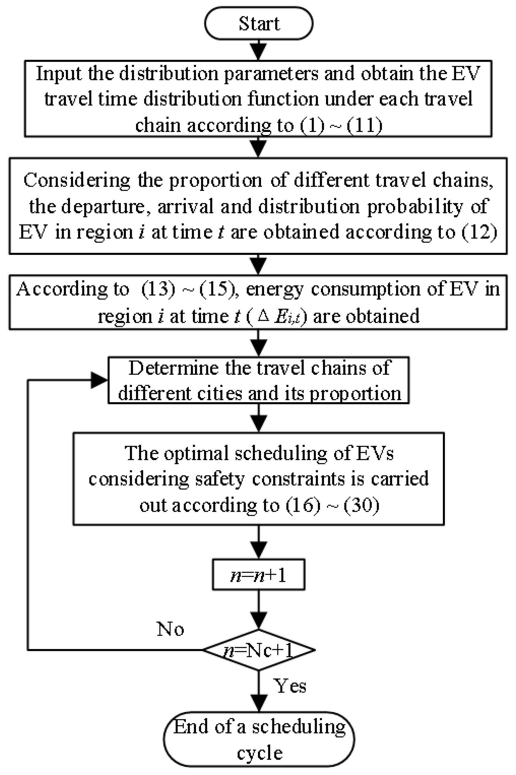
The scheduling strategy simulation process used in this paper was based on the EV and scheduling models of node clusters outlined in Section 2, Section 3 and Section 4 and is shown visually in Figure 3. First, we input the parameters required by the probability distribution function to obtain the travel conditions of EVs under each travel chain. We then used these functions to obtain the distribution of EVs in each region, including the departure and arrival probability distribution functions, by considering the proportion variables of each travel chain. Next, cities were classified into Nc cities according to the travel situation of urban residents, and we determined the proportion of EV users in various cities who were following each of our three predefined travel chains. Finally, we scheduled the charging and discharging of cluster EVs, accounting for the specific conditions of various cities as well as security constraints.

6. Results and Discussion

In this section, we compare and analyze our scheduling model based on the Institute of Electrical and Electronics Engineers (IEEE) 14-node distribution network system. We solved for the optimized scheduling model using the YALMIP and CPLEX toolboxes.

6.1. Basic Parameters

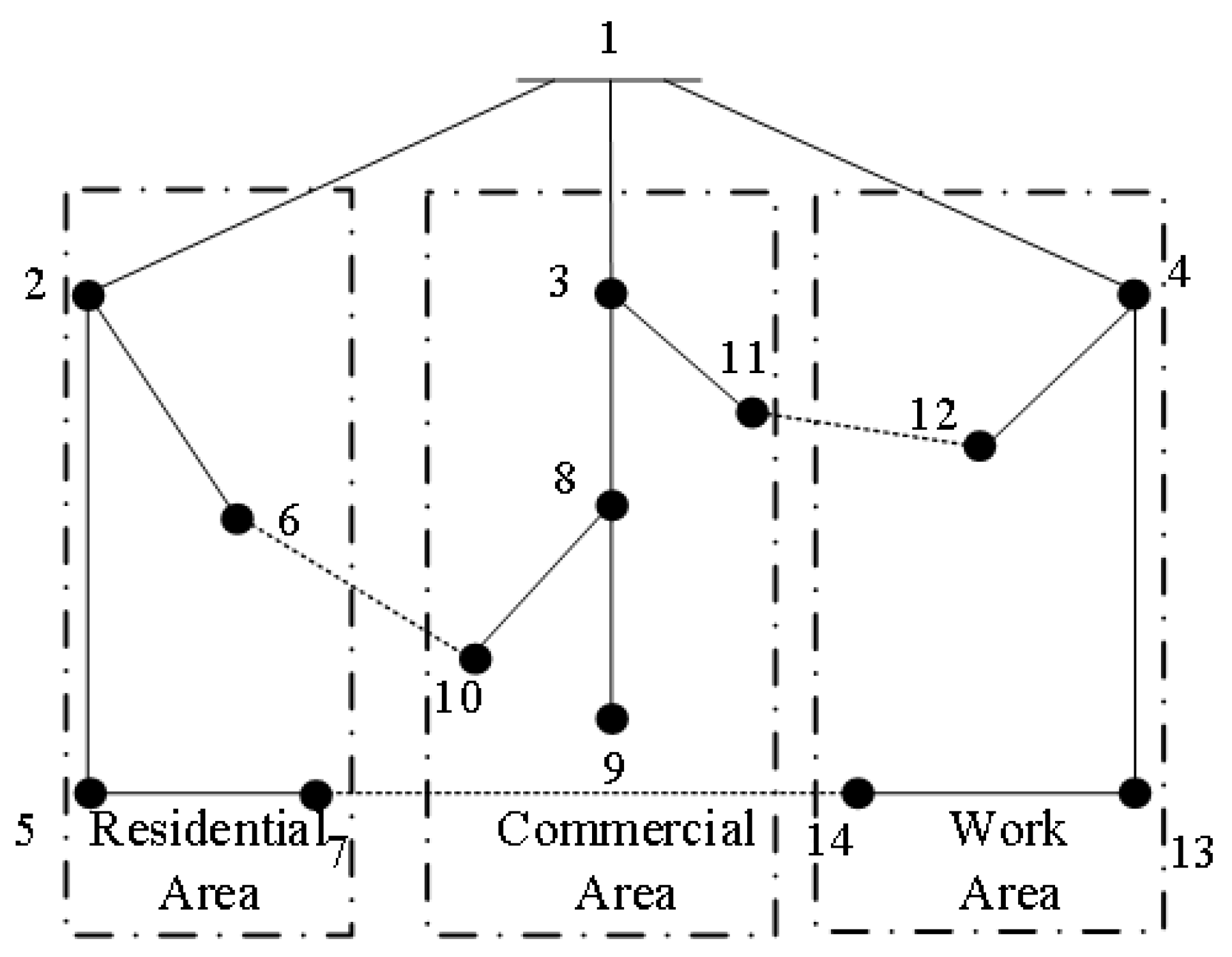
The IEEE 14-node distribution network system topology is shown in Figure 4. The distribution network has 13 branches with a reference voltage of 23 kV and a reference capacity of 100 MVA. The network parameters are as follows:

1.

The power factor of each node is 0.85, and the reactive power of the node is determined based on the active power injected into the node.

2.

All nodes, except for nodes 10 and 11, are equipped with EV charging stations. The total number of EVs is 2400. Other predefined parameters include L₁₂ = 15 km, L₂₃ = 12 km, L₁₃ = 12 km, v = 30 km/h, and the energy consumption factor E = 0.25. The network assumes that EVs are evenly distributed in the same functional area. The specific parameters of EVs are shown in

Table 2. Parameters of EVs in the model.

EV Battery Capacity (kWh)	Maximum SOC	Minimum SOC	Max Charging Power (kW)	Max Discharging Power (kW)	Demand SOC
24	0.95	0.2	15	15	Residential 0.9 Working 0.85 Commercial 0.85

.

3.

Electricity prices in Jiangsu Province are divided into three rates based on time of use (peak, normal, and valley). Prices for each usage period are shown in

Table 3. Electricity prices during different time periods.

Time	Peak (8:00–12:00; 17:00–21:00)	Normal (12:00–17:00; 21:00–24:00)	Valley (0:00–8:00)
Price (USD)	169.12	101.47	49.52

.

6.2. Comparison with Traditional Monte Carlo Sampling

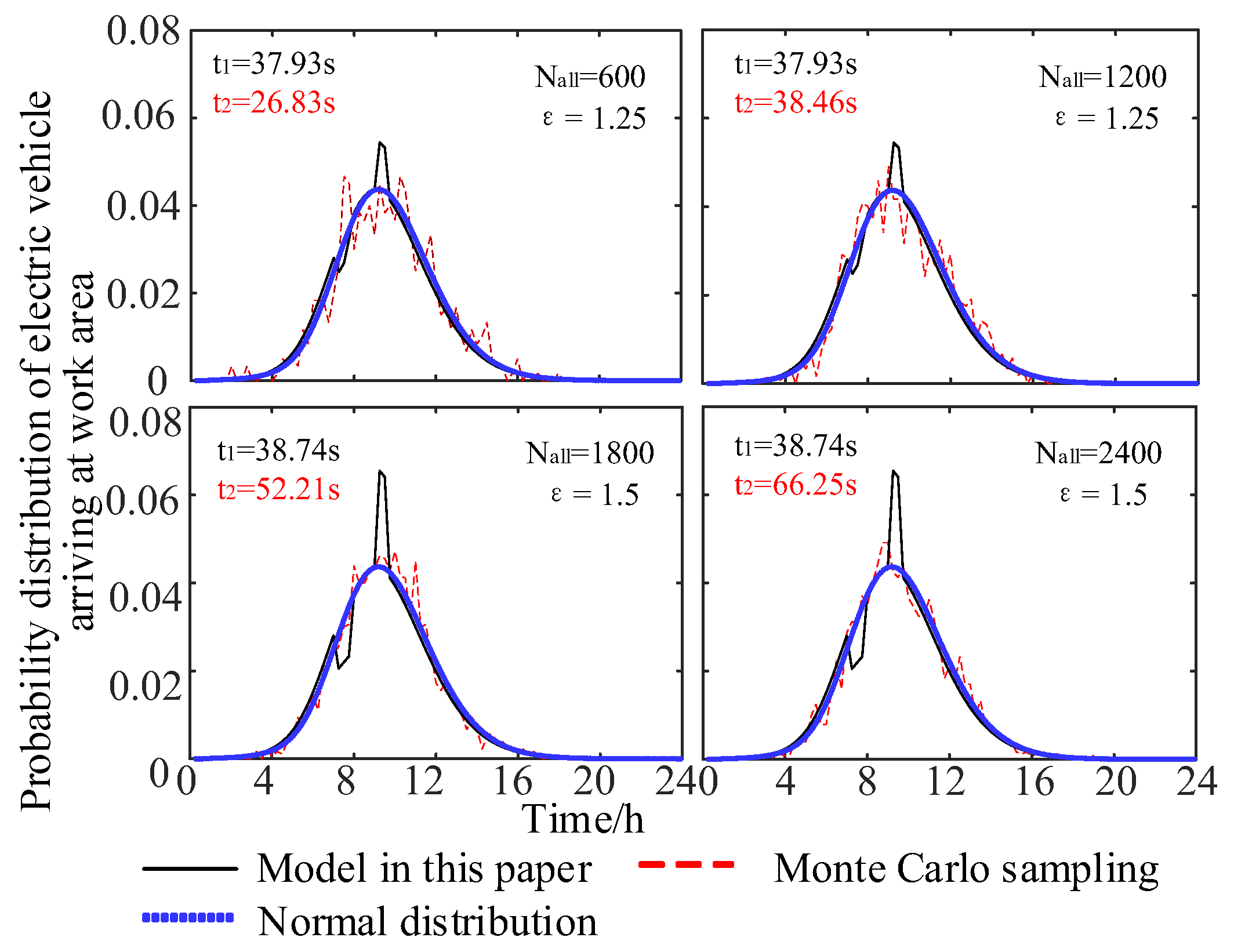
Most studies [8,9,10] obtain EV trip patterns by conducting Monte Carlo sampling of the departure and arrival times of EVs based on normal distribution rules. Figure 5 shows the probability distribution of the time EVs reach the working area in the simple work chain A (H–W–H). When the number of EVs is small, the time distribution obtained by Monte Carlo sampling is stochastic and volatile. As the number of cluster EVs increases, the computational time (t₂) required by the traditional Monte Carlo sampling method gradually increases, as shown in Figure 5. However, the resulting distribution gradually approaches uniformity. Given the increasing number of EVs in the current city and the uniform distribution pattern of cluster EVs, we therefore derived the probability distribution formula mathematically which uses less time (t₂) with the growth of the number of EVs.

In addition, our model fully accounts for traffic congestion. As shown in Figure 5, travel congestion shifts EV arrival times to the later part of the congestion period, and the probability of arriving at the working area peaks at 9:00. The congestion coefficient ε in our model can also be adjusted to match actual congestion in the city; for example, Figure 5 shows the probability distribution for congestion coefficients ε of 1.25 and 1.5.

6.3. Distribution of Electric Vehicles in Various Cities

As different cities are in different regions with different levels of economic development, pillar industries and residents’ lifestyles and travel rules vary among cities. The proportions of EV users following each of the three travel chains correspondingly vary among cities (i.e., the β_A, β_B and β_C parameters are different). In this study, we compared the following three urban travel chain models:

• Small cities, where simple work chain A and complex work chain B are considered but the work–entertainment chain C is absent (β_A = 30%, β_B = 70%, β_C = 0%).
• Large industrial cities: simple work chain A is more common than work–entertainment chain C (β_A = 70%, β_B = 0%, β_C = 30%).
• Large commercial cities: simple work chain A is less common than work–entertainment chain C (β_A = 30%, β_B = 0%, β_C = 70%).

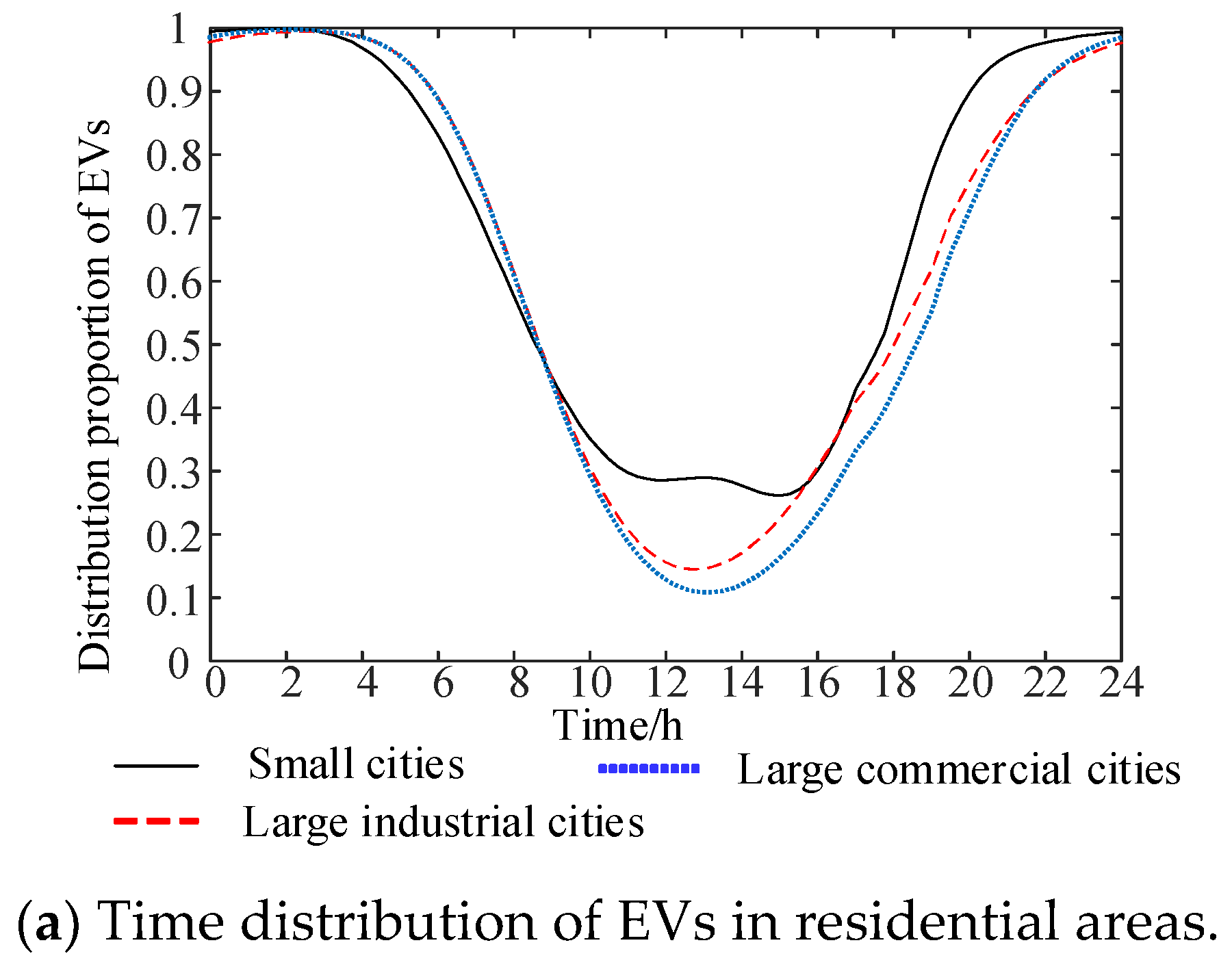
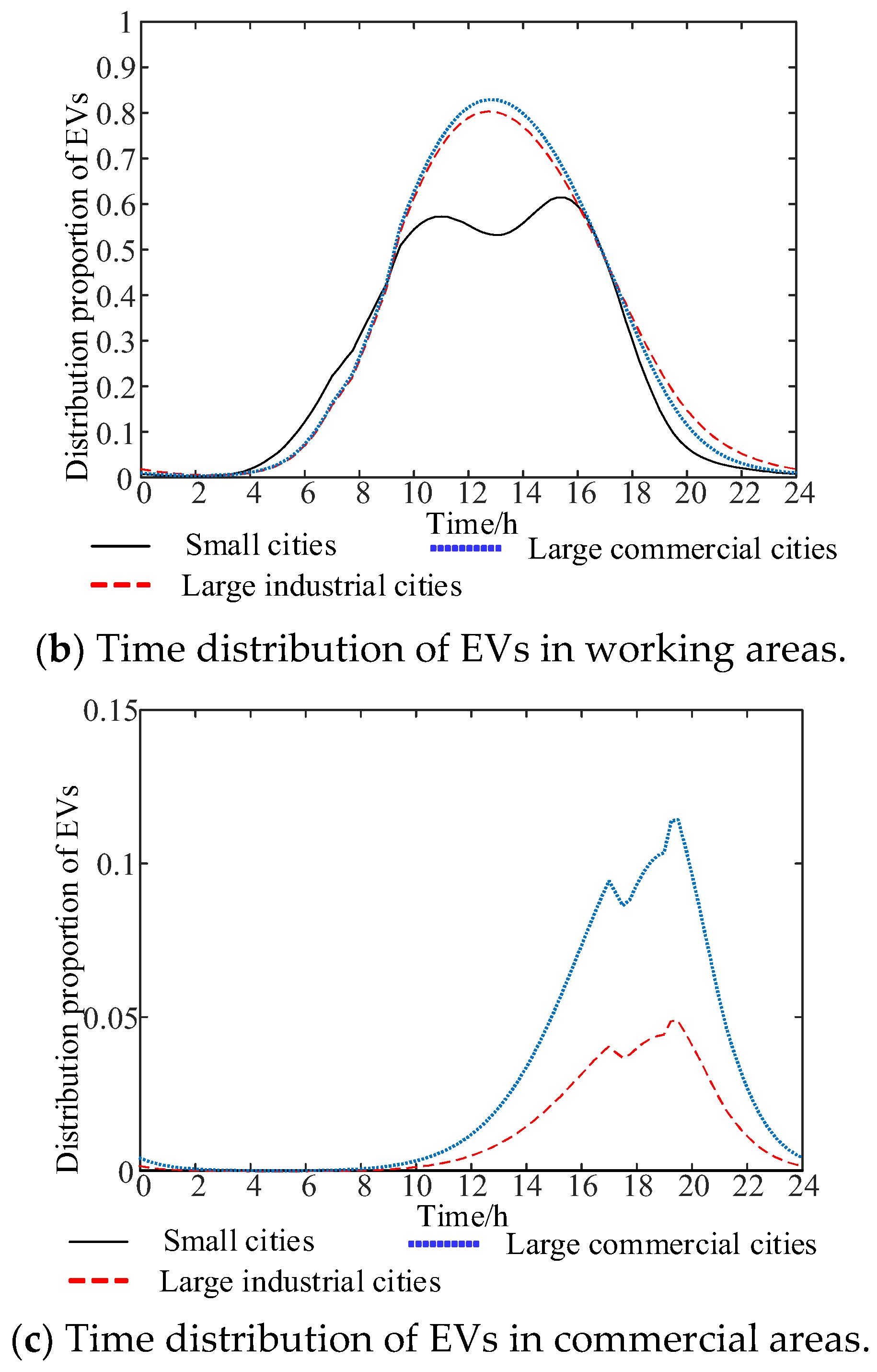
The probability distribution of EVs in these three different city types is shown in Figure 6.

Based on the idealized assumption that small cities have simple work chain A and complex work chain B, both of which do not have a work–entertainment trip, there is no work–entertainment chain in small cities. EVs are only distributed in working and residential areas. In addition, because some EV users in small cities return home for lunch, some EVs are transferred from working to residential areas during the lunch hour. In large cities, EV users make a trip for entertainment after work, so some electric vehicles are moved to the commercial area at night. Three distinct shifts can be observed as the proportion of H–W–E–H trips (i.e., the degree of commercialization) increases: (1) the proportion of EVs in residential areas from 12:00 to 22:00 decreases; (2) the proportion of EVs in commercial areas from 12:00 to 22:00 increases; and (3) more EVs in the working area are transferred to the commercial area from 17:00 to 22:00.

There is also a small fluctuation among in the distribution probability curves for EVs in the three regions. This fluctuation exists because our model accounts for traffic encountered in the actual travel process.

6.4. Charging and Discharging Scheduling Results of Electric Vehicles in Various Cities

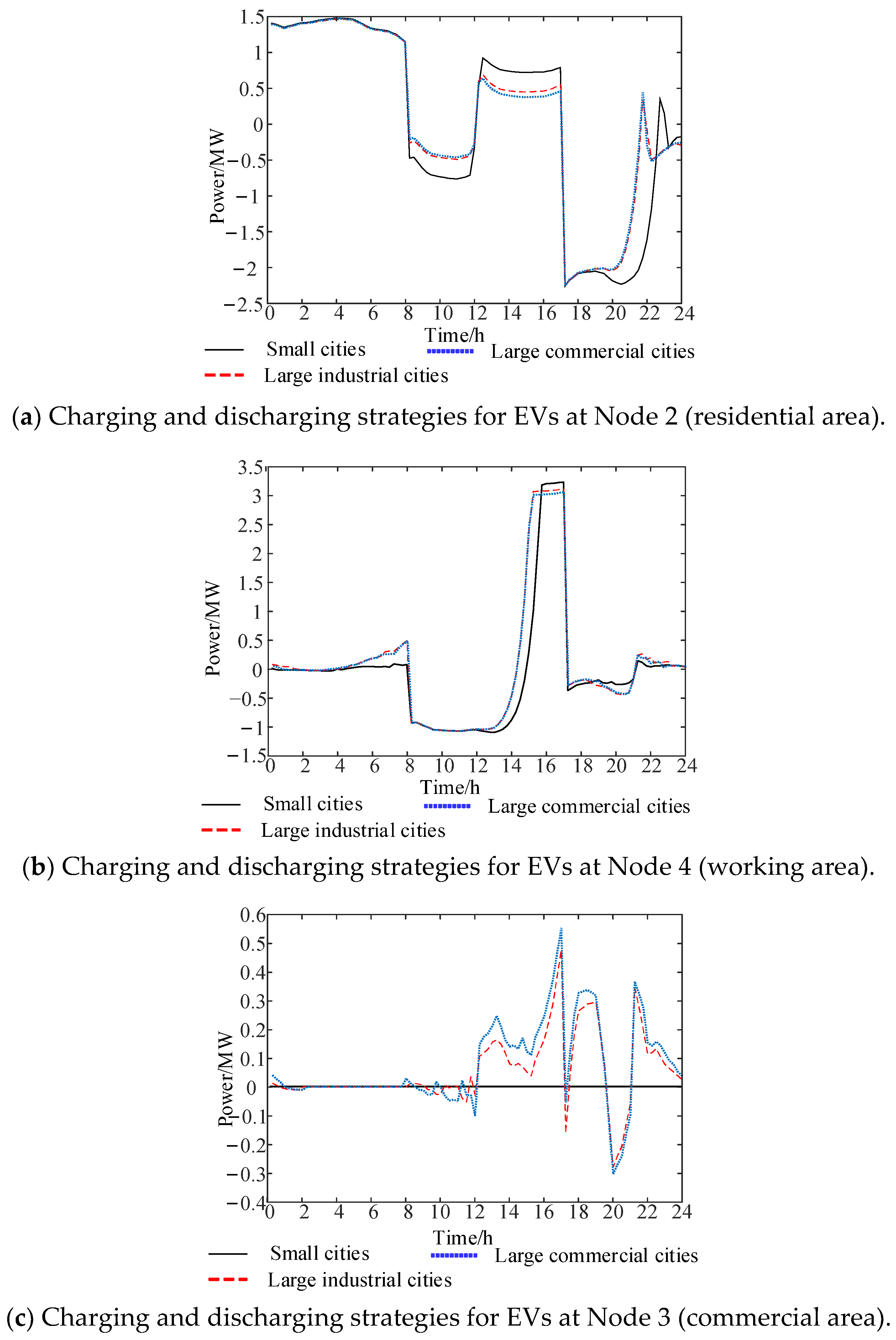
In this paper, we determined strategies for scheduling the charging and discharging of EVs in different functional areas of various cities by considering the optimization model of distribution network power flow, as shown in Figure 7.

Nodes 2, 3 and 4 represent residential, working, and commercial areas, respectively, for which we obtained the charging and discharging strategy of EVs, as shown in Figure 7. The distribution pattern of EVs in each region was fully considered when coordinating charging and discharging strategies. Charging and discharging strategies for EVs in residential areas make full use of the peak-valley electricity use pattern by charging at night to “fill” the valley and discharging during the evening (17:00 ~ 21:00) to relieve the peak load. The EVs in the working area discharge during the peak load period and charge during the normal load period so that they are fully charged for their next trip. The charging and discharging power of EVs in commercial areas fluctuates greatly because the residence time of EVs in commercial areas is shorter and more random.

In addition, because EVs remain in residential and working areas for long periods of time, V2G technology can be used to transmit power to the power grid during peak hours. Due to the shorter residence time of EVs in the commercial area (except for in small cities which lack a commercial area), EVs in commercial areas only release part of their power at approximately 20:00 to absorb the peak load.

Small cities have a larger charge and discharge limit at nodes 2 and 4, and can maintain charge for a longer amount of time, due to the proportion of EVs in residential and working areas. As the proportion of H–W–E–H trips increases, the charging and discharging range of residential and working areas becomes smaller, but the charging and discharging power range of commercial areas becomes larger. Although some nodes are in the same functional area (e.g., multiple nodes in residential areas), the scheduling strategies for different nodes are not the same because our model considers the power flow of the distribution network.

We lastly calculated the cost of the distribution network in various cities, and the profit of EVs in various regions, as shown in

Table 4. Costs of the distribution network and benefits of electric vehicles in different functional areas.

	Network Cost (USD)	EV Benefit (USD)	Benefit in Residential Areas (USD)	Benefit in Working Areas (USD)	Benefit in Commercial Areas (USD)
Small cities	72,090	6781	4576	2197	0
Large industrial cities	74,538	4432	3527	1449	−226
Large commercial cities	74,688	4270	3517	1332	−579

:

Costs of the distribution network and benefits of EVs are demonstrated in this table. Cost of the network is the optimal result of target function (20). EV benefits (or arbitrage) in total, as well as benefits in different functional areas are achieved through calculating the difference between cost and profits of EVs in the corresponding areas. Note that the cost of the distribution network is lower, and the benefit of EVs is higher in small cities relative to the two large cities. This is because the higher proportion of EVs in residential and working areas can take full advantage of the peak–valley electricity pricing system. Industrial cities are second for both costs and benefits. EVs in commercial cities have the highest cost and the lowest profit because they have more entertainment trips. There is a large amount of randomness in the E–H trip and a short stay time in the commercial area; EVs are mainly charged in the commercial area, thus limiting the efficiency of the V2G strategy for EVs.

7. Conclusions

This paper develops a charging–discharging operation strategy for electric vehicles based on different trip patterns for various city types. Considering the different travel chain patterns of EVs, we deduced the probability density function for the spatiotemporal distribution of EVs while accounting for travel time, traffic congestion, and journey energy consumption. In addition, as different EV users in different types of cities have different travel patterns, the spatiotemporal distribution of EVs differs among functional areas. Therefore, we also obtained the distribution of EVs in different cities, where different travel chains represent different proportions of EV user travel habits. Based on our time and space distribution model, we combined the power flow and voltage constraints of the distribution network with the goal of economically optimizing charging–discharging strategies of EVs at each node in each region.

The key findings of this paper include:

• The time distribution obtained by Monte Carlo sampling is stochastic and volatile, so we derived the probability distribution formula of EVs mathematically based on different travel chain patterns of EVs in different cities.
• In our proposed scheduling strategy, the distribution pattern of EVs in each region was fully considered when coordinating charging and discharging strategies. Furthermore, scheduling results differ among different types of cities due to the different proportions of EVs in different regions at different time periods.
• The cost of the distribution network is minimized, and the profit of EVs is maximized in small cities. EVs prefer charging rather than discharging in commercial areas, limiting the efficiency of the V2G strategy for EVs in commercial areas. Therefore, EVs in commercial cities have the highest cost and the lowest profit, and the power grid economy is relatively low.

References

- Mukherjee, J.C.; Gupta, A. A Review of Charge Scheduling of Electric Vehicles in Smart Grid. IEEE Syst. J. 2015, 9, 1541–1553. [Google Scholar] [CrossRef]
- Nimalsiri, N.I.; Mediwaththe, C.P.; Ratnam, E.L.; Shaw, M.; Smith, D.B.; Halgamuge, S.K. A Survey of Algorithms for Distributed Charging Control of Electric Vehicles in Smart Grid. IEEE Trans. Intell. Transp. Syst. 2020, 21, 4497–4515. [Google Scholar] [CrossRef] [Green Version]
- Cao, Y.; Wang, T.; Kaiwartya, O.; Min, G.; Ahmad, N.; Abdullah, A.H. An EV Charging Management System Concerning Drivers’ Trip Duration and Mobility Uncertainty. IEEE Trans. Syst. Man Cybern. Syst. 2018, 48, 596–607. [Google Scholar] [CrossRef] [Green Version]
- Chaudhari, K.; Ukil, A.; Kumar, K.N.; Manandhar, U.; Kollimalla, S.K. Hybrid Optimization for Economic Deployment of ESS in PV-Integrated EV Charging Stations. IEEE Trans. Ind. Inform. 2018, 14, 106–116. [Google Scholar] [CrossRef]
- Franco, J.F.; Rider, M.J.; Romero, R. A Mixed-Integer Linear Programming Model for the Electric Vehicle Charging Coordination Problem in Unbalanced Electrical Distribution Systems. IEEE Trans. Smart Grid 2015, 6, 2200–2210. [Google Scholar] [CrossRef]
- Xu, S.; Feng, D.; Yan, Z.; Zhang, L.; Li, N.; Jing, L.; Wang, J. Ant-Based Swarm Algorithm for Charging Coordination of Electric Vehicles. Int. J. Distrib. Sens. Netw. 2013, 9, 268942. [Google Scholar] [CrossRef]
- Qi, W.; Xu, Z.; Shen, Z.-J.M.; Hu, Z.; Song, Y. Hierarchical Coordinated Control of Plug-in Electric Vehicles Charging in Multifamily Dwellings. IEEE Trans. Smart Grid 2014, 5, 1465–1474. [Google Scholar] [CrossRef]
- Zhou, J.; Jiang, H.; Zhang, X.; Li, Z.; Pang, J. Electric Vehicle Travel Chain Model and Case Analysis Based on Time and Space Characteristics. In Proceedings of the 2019 IEEE Sustainable Power and Energy Conference (iSPEC), Beijing, China, 21–23 November 2019; pp. 1535–1539. [Google Scholar]
- Moghaddass, R.; Mohammed, O.A.; Skordilis, E.; Asfour, S. Smart Control of Fleets of Electric Vehicles in Smart and Connected Communities. IEEE Trans. Smart Grid 2019, 10, 6883–6897. [Google Scholar] [CrossRef]
- He, Y.; Venkatesh, B.; Guan, L. Optimal Scheduling for Charging and Discharging of Electric Vehicles. IEEE Trans. Smart Grid 2012, 3, 1095–1105. [Google Scholar] [CrossRef]
- Tang, Y.; Zhong, J.; Bollen, M. Aggregated optimal charging and vehicle-to-grid control for electric vehicles under large electric vehicle population. IET Gener. Transm. Distrib. 2016, 10, 2012–2018. [Google Scholar] [CrossRef]
- Yuan, Z.; Yu, L.; Xu, Q.; Zou, C.; Qv, K.; Xu, S.; Yin, S. Optimization of Orderly Charge and Discharge Scheduling of Electric Vehicles and Photovoltaic in Industrial Par. In Proceedings of the 2020 Asia Energy and Electrical Engineering Symposium (AEEES), Chengdu, China, 29–31 May 2020; pp. 226–229. [Google Scholar]
- Liang, H.; Lee, Z.; Li, G. A Calculation Model of Charge and Discharge Capacity of Electric Vehicle Cluster Based on Trip Chain. IEEE Access 2020, 8, 142026–142042. [Google Scholar] [CrossRef]
- U.S. Department of Transportation, Federal Highway Administration. 2017 National Household Travel Survey [EB/OL]. Available online: http://nhts.ornl.gov (accessed on 28 October 2021).
- UK Department for Transport. National Travel Survey: 2016. [EB/OL]. Available online: html://https://www.gov.uk/government/statistics/national-travel-survey-2016 (accessed on 28 October 2021).
- Xu, W. Understanding the Intra-urban Residents’ Trip Characteristics Based on GPS. In Proceedings of the 2019 IEEE 19th International Conference on Communication Technology (ICCT), Xi’an, China, 16–19 October 2019; pp. 1555–1559. [Google Scholar]
- Zhenru, L.; Xuemei, L.I. Review of trip-chain-based travel activity study of residents. In Proceedings of the 2010 International Conference on Logistics Systems and Intelligent Management (ICLSIM), Harbin, China, 9–10 January 2010; pp. 1527–1531. [Google Scholar]
- Xue, M. Cangnan Inhabitant Trips Characteristics Study. Traffic Transp. 2009, 12, 7–10. [Google Scholar]
- Chen, Z.; Zhang, Z.; Zhao, J.; Wu, B.; Huang, X. An Analysis of the Charging Characteristics of Electric Vehicles Based on Measured Data and Its Application. IEEE Access 2018, 6, 24475–24487. [Google Scholar] [CrossRef]
- Neumanenn, F. Optimal Scheduling of EV Charging in Distribution Networks. Master’s Thesis, The University of Edinburgh, Edinburgh, Scotland, 2017. [Google Scholar]