
Optimal Design of a Short Primary Double-Sided Linear Induction Motor for Urban Rail Transit


Abstract
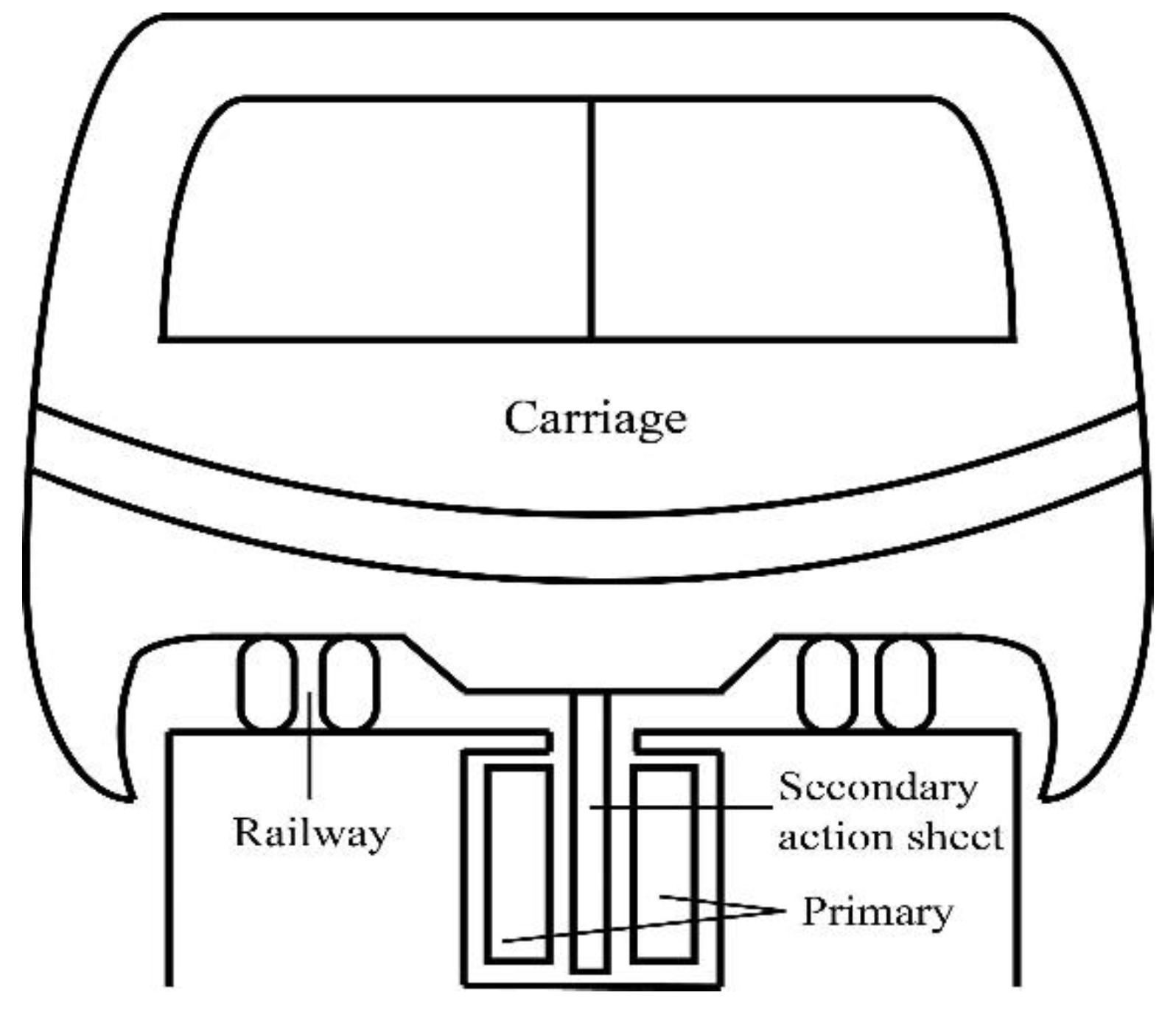
:1. Introduction
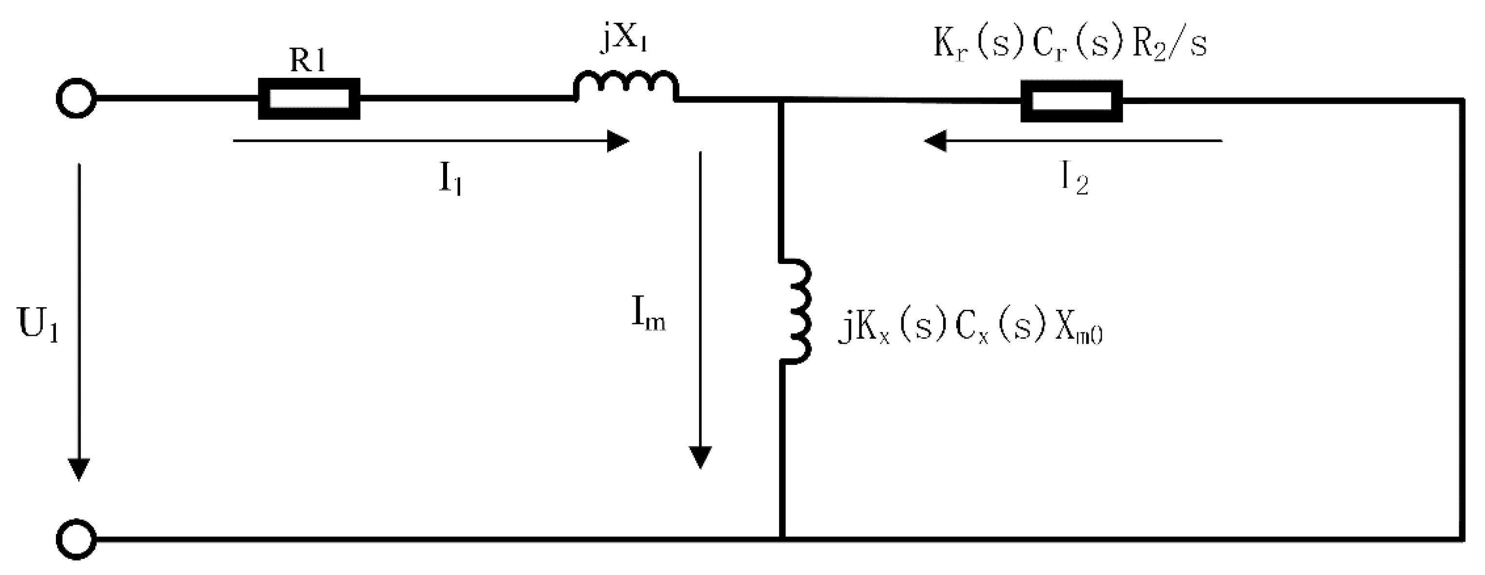
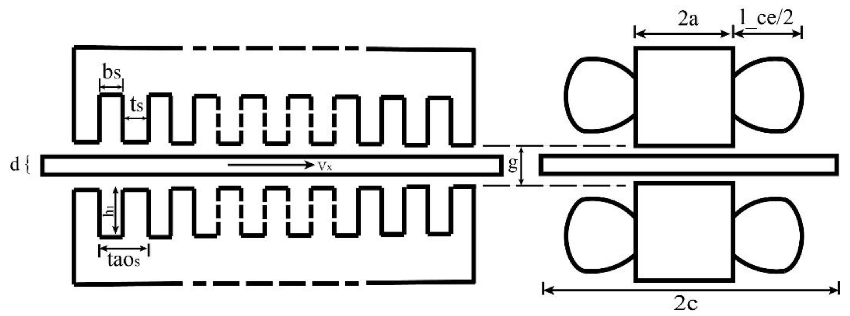
2. Equivalent Circuit of the Short Primary Double-Sided Linear Induction Motor
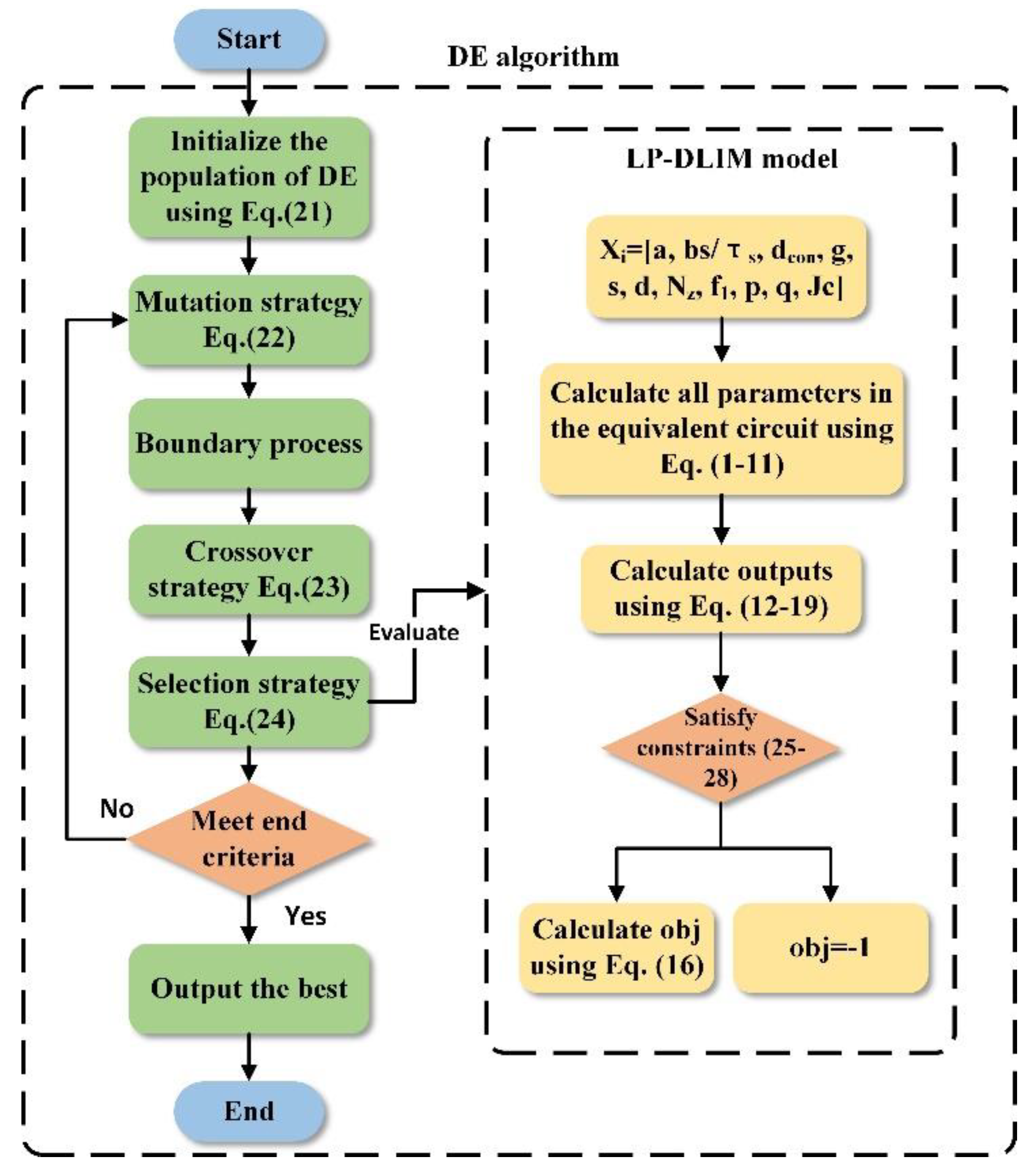
3. Design Optimization Process
3.1. Main Indicators of SP-DLIM
3.2. Parameter Search Range of the Optimal Design
3.2.1. Initialization
3.2.2. Mutation
3.2.3. Crossover
3.2.4. Selection
3.3. Process of the Optimal Design
4. Optimal Results and FEM validation
4.1. Optimal Results
4.1.1. Operating Rules of DE Algorithm
- Crossover rate is 0.5;
- Scaling factor is set as a randomly distributed number for every individual;
- Population size is set as 50.
4.1.2. Optimal Results
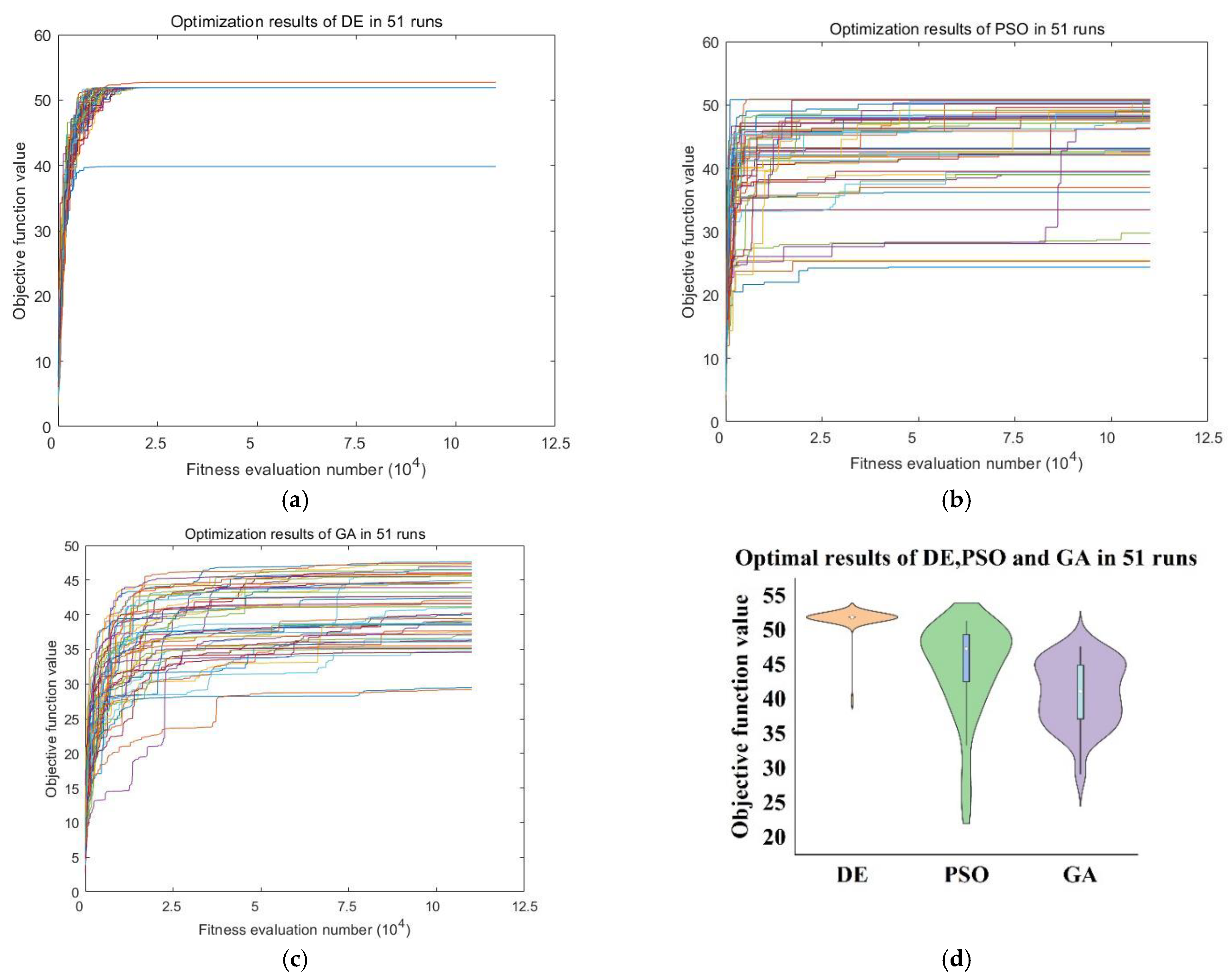
4.1.3. Comparison Results between DE, PSO, and GA
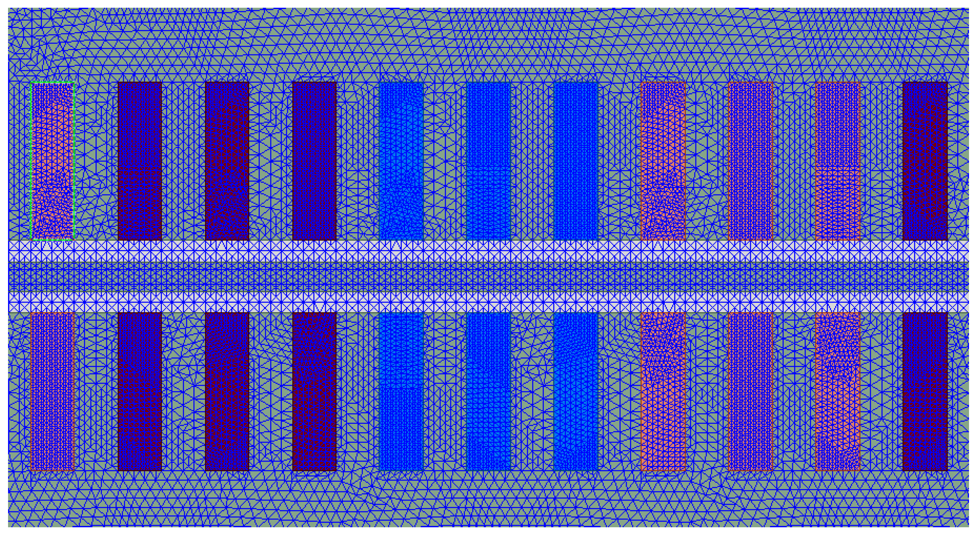
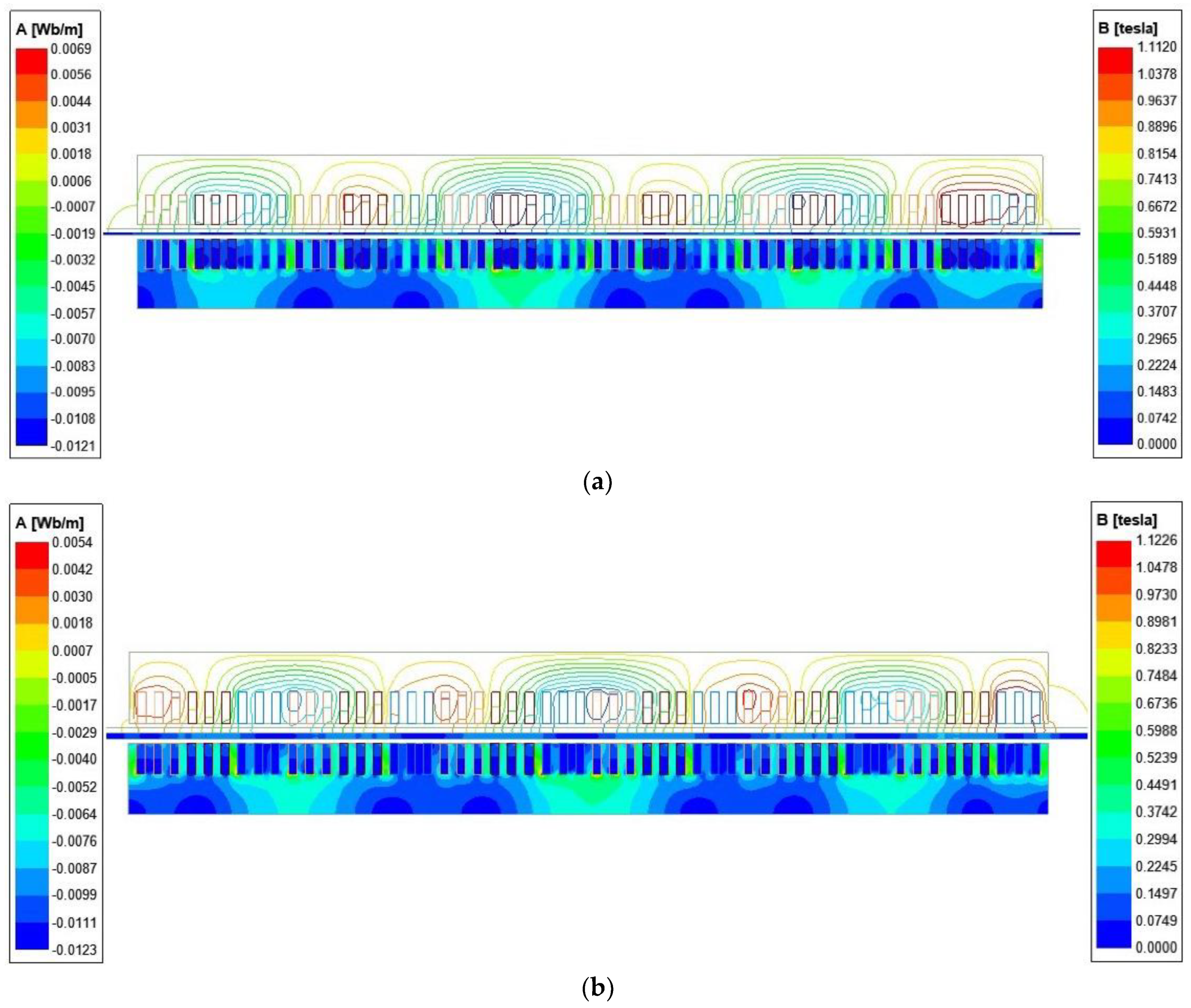
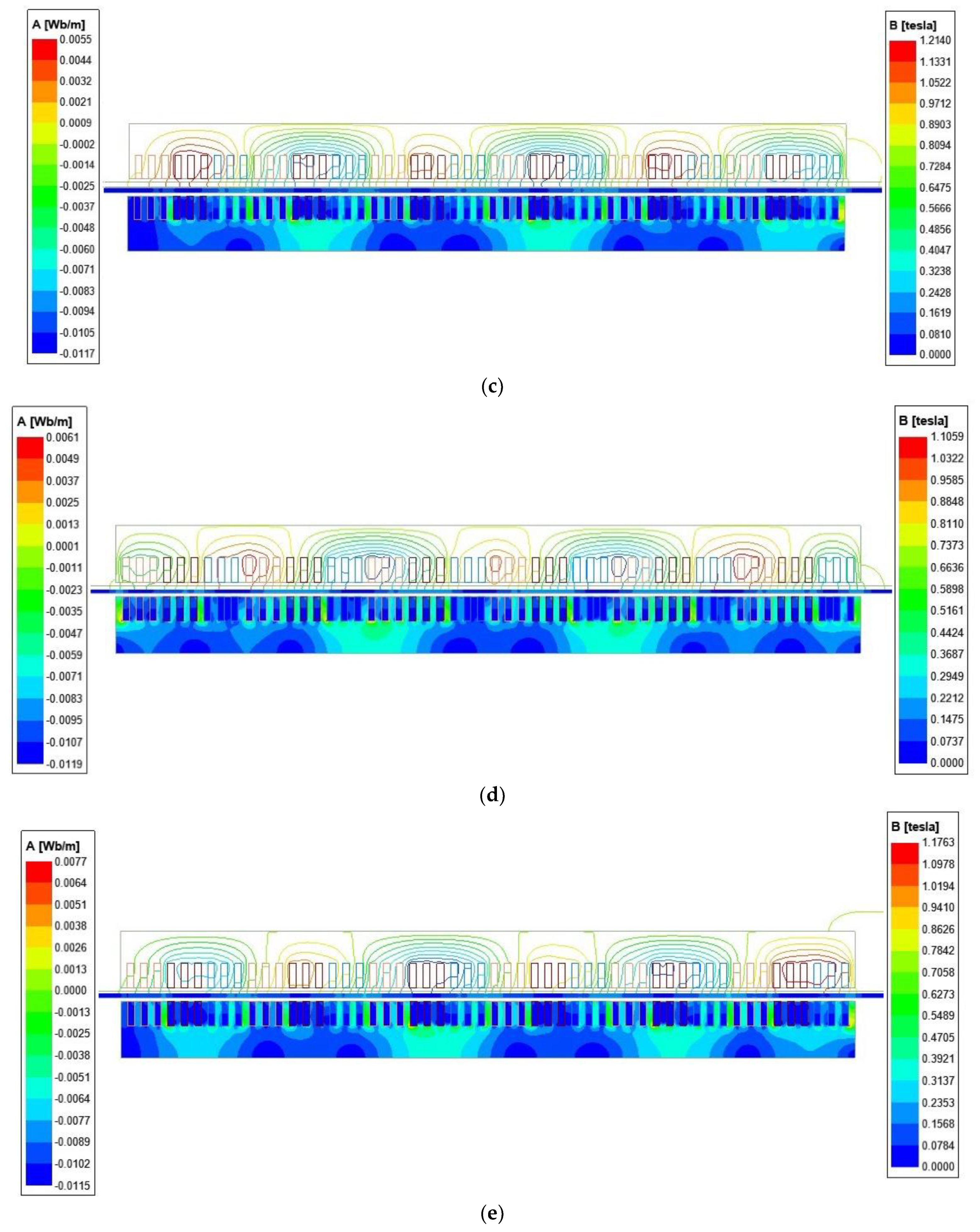
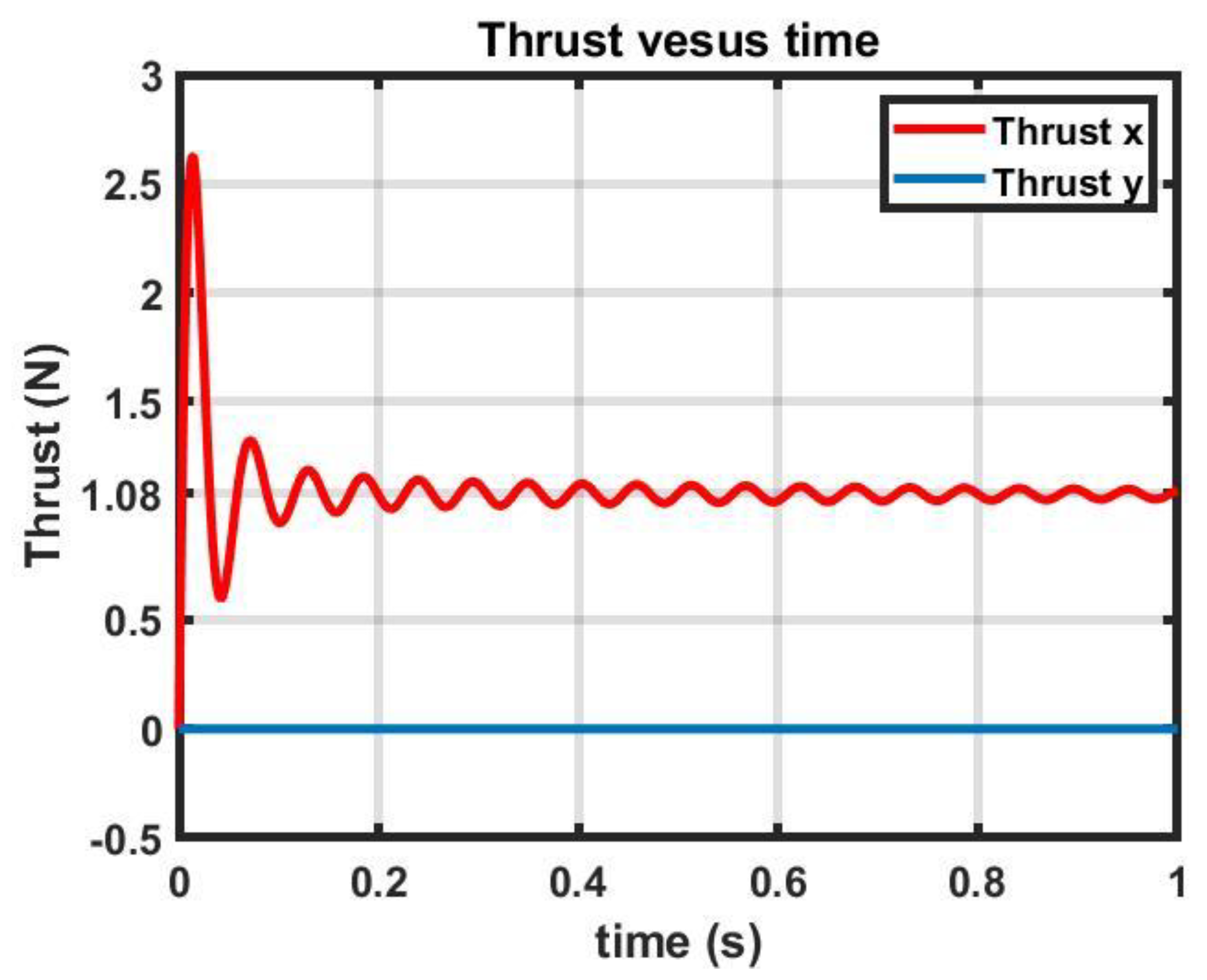
4.2. 2-D transient FEM Simulation Results
5. Discussion
6. Conclusions
Author Contributions
Funding
Institutional Review Board Statement
Informed Consent Statement
Conflicts of Interest
References
- Lu, J.; Ma, W. Research on End Effect of Linear Induction Machine for High-Speed Industrial Transportation. IEEE Trans. Plasma Sci. 2011, 39, 116–120. [Google Scholar] [CrossRef]
- Nonaka, S.; Higuchi, T. Elements of linear induction motor design for urban transit. IEEE Trans. Magn. 1987, 23, 3002–3004. [Google Scholar] [CrossRef]
- Xu, W.; Zhu, J.; Tan, L.; Guo, Y.; Wang, S.; Wang, Y. Optimal design of a linear induction motor applied in transportation. In Proceedings of the 2009 IEEE International Conference on Industrial Technology, Churchill, VIC, Australia, 10–13 February 2009; pp. 1–6. [Google Scholar]
- Solomin, V.A.; Solomin, A.V.; Zamshina, L.L. Mathematical Modeling of Currents in Secondary Element of Linear Induction Motor with Transverse Magnetic Flux for Magnetic-Levitation Transport. In Proceedings of the 2019 International Conference on Industrial Engineering, Applications and Manufacturing (ICIEAM), Sochi, Russia, 25–29 March 2019; pp. 1–6. [Google Scholar] [CrossRef]
- Ruihua, Z.; Yumei, D.; Yaohua, L.; Ke, W.; Huamin, Q. Experimental research of linear induction motor for urban mass transit. In Proceedings of the 2010 International Conference on Electrical Machines and Systems, Incheon, Korea, 10–13 October 2010; pp. 1524–1527. [Google Scholar]
- Cho, H.T.; Liu, Y.C.; Kim, K.A. Short-Primary Linear Induction Motor Modeling with End Effects for Electric Transportation Systems. In Proceedings of the 2018 International Symposium on Computer, Consumer and Control (IS3C), Taichung, Taiwan, 6–8 December 2018; pp. 338–341. [Google Scholar] [CrossRef]
- Lv, G.; Zhou, T.; Zeng, D.; Liu, Z. Influence of Secondary Constructions on Transverse Forces of Linear Induction Motors in Curve Rails for Urban Rail Transit. IEEE Trans. Ind. Electron. 2019, 66, 4231–4239. [Google Scholar] [CrossRef]
- Abdollahi, S.E.; Mirzayee, M.; Mirsalim, M. Design and Analysis of a Double-Sided Linear Induction Motor for Transportation. IEEE Trans. Magn. 2015, 51, 1–7. [Google Scholar] [CrossRef]
- Long, X. The Theory and Electromagnetic Design Method of Linear Induction Motors; Science Press: Beijing, China, 2006. [Google Scholar]
- Boldea, I. Linear Electric Machines, Drives, and MAGLEVs Handbook; CRC Press: Boca Raton, FL, USA, 2013. [Google Scholar]
- Duncan, J. Linear induction motor-equivalent circuit model. Proc. IEEE 1983, 130, 51–57. [Google Scholar]
- Osawa, S.; Wada, M.; Karita, M.; Ebihara, D.; Yokoi, T. Light-weight type linear induction motor and its characteristics. IEEE Trans. Magn. 1992, 28, 3003–3005. [Google Scholar] [CrossRef]
- Laporte, B.; Takorabet, N.; Vinsard, G. An approach to optimize winding design in linear induction motors. IEEE Trans. Magn. 1997, 33, 1844–1847. [Google Scholar] [CrossRef]
- Hassanpour Isfahani, A.; Ebrahimi, B.M.; Lesani, H. Design optimization of a low speed single-sided linear induction motor for improved efficiency and powerfactor. IEEE Trans. Magn. 2008, 44, 266–272. [Google Scholar] [CrossRef]
- Lucas, C.; Nasiri-Gheidari, Z.; Tootoonchian, F. Application of an imperialist competitive algorithm to design of linear induction motor. Energy Convers. Manag. 2010, 51, 1407–1411. [Google Scholar] [CrossRef]
- Bazghaleh, A.Z.; Naghashan, M.R.; Meshkatoddini, M.R. Optimum design of single sided linear induction motors for improved motor performance. IEEE Trans. Magn. 2010, 46, 3939–3947. [Google Scholar] [CrossRef]
- Bazghaleh AZare Naghashan, M.R.; Meshkatoddini, M.R.; Mahmoudimanesh, H. Optimum design of high speed single-sided linear induction motor to obtain best performance. In Proceedings of the SPEEDAM 2010, Pisa, Italy, 14–16 June 2010. [Google Scholar]
- Zhao, J.; Zhang, W.; Fang, J.; Yang, Z.; Zheng, Q.T.; Liu, Y. Design of HTS Linear Induction Motor using GA and the Finite Element Method. In Proceedings of the 2010 5th IEEE Conference on Industrial Electronics and Applications, Taichung, Taiwan, 15–17 June 2010. [Google Scholar] [CrossRef]
- Shiri, A.; Shoulaie, A. End effect braking force reduction in high-speed single-sided linear induction machine. Energy Convers. Manag. 2012, 61, 43–50. [Google Scholar] [CrossRef]
- Xu, W.; Zhu, J.G.; Zhang, Y.; Li, Y.; Wang, Y.; Guo, Y. An Improved Equivalent Circuit Model of a Single-Sided Linear Induction Motor. IEEE Trans. Veh. Technol. 2010, 59, 2277–2289. [Google Scholar] [CrossRef] [Green Version]
- Lv, G.; Zeng, D.; Zhou, T. An Advanced Equivalent Circuit Model for Linear Induction Motors. IEEE Trans. Ind. Electron. 2018, 65, 7495–7503. [Google Scholar] [CrossRef]
- Yang, T.; Zhou, L.; Li, L. Influence of Design Parameters on End Effect in Long Primary Double-Sided Linear Induction Motor. IEEE Trans. Plasma Sci. 2011, 39, 192–197. [Google Scholar] [CrossRef]
- Yang, T.; Zhou, L.; Li, L. Performance calculation for double-sided linear induction motor with short secondary. In Proceedings of the 2008 International Conference on Electrical Machines and Systems, Wuhan, China, 17–20 October 2008; pp. 3478–3483. [Google Scholar]
- Das, S.; Suganthan, P.N. Differential Evolution: A Survey of the State-of-the-Art. IEEE Trans. Evol. Comput. 2011, 15, 4–31. [Google Scholar] [CrossRef]
- Guohua, W.; Rammohan, M.; Suganthan, P. Problem Definitions and Evaluation Criteria for the CEC 2017 Competition and Special Session on Constrained Single Objective Real-Parameter Optimization; Nanyang Technological Universityr: Singapore, 2016. [Google Scholar]
- Davis, L. Handbook of Genetic Algorithms; Van Nostrand Reinhold: New York, NY, USA, 1990. [Google Scholar]
- Poli, R.; Kennedy, J.; Blackwell, T.M. Particle swarm optimization. Swarm Intell. 2007, 1, 33–57. [Google Scholar] [CrossRef]


| Line Voltage | 500 V |
| Rated thrust | 1.1 kN ± 5% |
| Rated speed | 45 Km/h |
| Winding layer | 1 |
| Design Parameters | Min. Value | Max. Value | Unit |
|---|---|---|---|
| 0.05 | 0.15 | m | |
| 0.3 | 0.5 | - | |
| 0.5 | 1.5 | mm | |
| 10 | 30 | mm | |
| 4 | 10 | mm | |
| 0.1 | 0.5 | - | |
| 3 | 6 | A/mm2 | |
| 1 | 200 | Hz | |
| 3 | 10 | - | |
| 1 | 3 | - | |
| 10 | 100 | - |
| Type | Parameters | Unit | Optimal Results | |
|---|---|---|---|---|
| Design parameters | Primary stack width (a) | mm | 85.8 | |
| Slot width/slot pitch (bs/τs) | - | 0.5 | ||
| Conductor diameter (dcon) | mm | 1.5 | ||
| Number of turns per slot (Nz) | - | 52 | ||
| Number of slots/pole/phase (q) | - | 3 | ||
| Number of pole pairs (p) | - | 3 | ||
| Supply power frequency (f1) | Hz | 76.18 | ||
| Primary current density (Jc) | A/m2 | 6 × 10⁶ | ||
| Slip (s) | - | 0.24 | ||
| Secondary thickness (d) | mm | 4 | ||
| Air gap length (g) | mm | 10 | ||
| Equivalent circuit parameters | Slot width (bs) | mm | 6 | |
| Tooth width (ts) | mm | 6 | ||
| Pole pitch (τ) | m | 0.108 | ||
| Line voltage (U1) | V | 500 | ||
| Primary turns per phase (Nph) | - | 468 | ||
| Primary current (I1) | A | 21.21 | ||
| Phase winding resistance (R1) | Ω | 0.73 | ||
| Phase winding leakage reactance (X1) | mH | 12.5 | ||
| Slot height (h1) | mm | 21.7 | ||
| Goodness factor (G) | - | 10.1 | ||
| Output characteristics | Efficiency (η) | % | Mean | 71.87 |
| Best/Optimal | 73.29/71.74 | |||
| Power factor (pf) | % | Mean | 61.01 | |
| Best/Optimal | 63.16/61.11 | |||
| Thrust (Fem) | N × 103 | Mean | 1.12 | |
| Best/Optimal | 1.18/1.12 | |||
| Tooth weight | kg | Mean | 9.51 | |
| Best/Optimal | 9.25/9.45 | |||
| Objective function value | - | Mean Best/Optimal | 51.53 52.66/51.91 | |
| OFV | DE | PSO | GA | F = 0.2 | F = 0.3 | F = 0.4 | F = 0.5 | F = 0.6 | F = 0.7 | F = 0.8 | F = 0.9 |
| Successful rate | 100% | 64.71% | 43.14% | 94% | 100% | 100% | 47.06% | 100% | 100% | 100% | 100% |
| Best | 52.66 | 50.89 | 48.86 | 53.13 | 52.24 | 52.15 | 51.76 | 51.91 | 52.66 | 52.66 | 53.14 |
| Worst | 39.81 | 24.40 | 30.16 | 40.40 | 39.81 | 49.84 | 24.36 | 51.91 | 51.91 | 51.91 | 51.91 |
| mean | 51.68 | 43.59 | 40.33 | 50.77 | 51.17 | 51.74 | 42.46 | 51.91 | 51.94 | 52.00 | 52.00 |
| Std | 1.70 | 7.35 | 4.14 | 1.99 | 1.87 | 0.59 | 7.33 | 0 | 0.15 | 0.24 | 0.29 |
| OFV | F = 1 | CR = 0.1 | CR = 0.2 | CR = 0.3 | CR = 0.4 | CR = 0.5 | CR = 0.6 | CR = 0.7 | CR = 0.8 | CR = 0.9 | CR = 1 |
| Successful rate | 100% | 98% | 98% | 100% | 100% | 100% | 98% | 100% | 100% | 100% | 94% |
| Best | 53.12 | 52.25 | 52.31 | 52.64 | 52.66 | 52.66 | 52.91 | 53.14 | 53.14 | 53.14 | 53.14 |
| Worst | 48.33 | 49.02 | 51.70 | 51.81 | 51.91 | 51.91 | 39.81 | 51.91 | 39.81 | 39.81 | 33.47 |
| mean | 51.99 | 51.4 | 51.91 | 51.97 | 51.95 | 51.95 | 51.72 | 51.96 | 50.78 | 50.35 | 47.35 |
| Std | 0.58 | 0.84 | 0.11 | 0.19 | 0.18 | 0.18 | 1.71 | 0.22 | 3.89 | 4.54 | 6.43 |
| Characteristics | Optimal Results | FEM | Relative Error |
| Phase current | 21.21 A | 21.5 A | 1.3% |
| Thrust | 1117 N | 1076 kN | 3.8% |
| Efficiency | 71.84% | 71.09% | 1.1% |
Publisher’s Note: MDPI stays neutral with regard to jurisdictional claims in published maps and institutional affiliations. |
© 2022 by the authors. Licensee MDPI, Basel, Switzerland. This article is an open access article distributed under the terms and conditions of the Creative Commons Attribution (CC BY) license (https://creativecommons.org/licenses/by/4.0/).
Share and Cite
Wang, H.; Zhao, J.; Xiong, Y.; Xu, H.; Yan, S. Optimal Design of a Short Primary Double-Sided Linear Induction Motor for Urban Rail Transit. World Electr. Veh. J. 2022, 13, 30. https://doi.org/10.3390/wevj13020030
Wang H, Zhao J, Xiong Y, Xu H, Yan S. Optimal Design of a Short Primary Double-Sided Linear Induction Motor for Urban Rail Transit. World Electric Vehicle Journal. 2022; 13(2):30. https://doi.org/10.3390/wevj13020030
Chicago/Turabian StyleWang, Hanming, Jinghong Zhao, Yiyong Xiong, Hao Xu, and Sinian Yan. 2022. "Optimal Design of a Short Primary Double-Sided Linear Induction Motor for Urban Rail Transit" World Electric Vehicle Journal 13, no. 2: 30. https://doi.org/10.3390/wevj13020030
APA StyleWang, H., Zhao, J., Xiong, Y., Xu, H., & Yan, S. (2022). Optimal Design of a Short Primary Double-Sided Linear Induction Motor for Urban Rail Transit. World Electric Vehicle Journal, 13(2), 30. https://doi.org/10.3390/wevj13020030