Article

Prediction for the Remaining Useful Life of Lithium–Ion Battery Based on RVM-GM with Dynamic Size of Moving Window

School of Mechanical Engineering, Beijing Institute of Technology, Beijing 100000, China
*
Author to whom correspondence should be addressed.
World Electr. Veh. J. 2022, 13(2), 25; https://doi.org/10.3390/wevj13020025
Submission received: 23 December 2021 / Revised: 17 January 2022 / Accepted: 18 January 2022 / Published: 19 January 2022

Abstract

:
Accurate prediction of the remaining useful life of a lithium–ion battery (LiB) is of paramount importance for ensuring its durable operation. To achieve more accurate prediction with limited data, this paper proposes an RVM-GM algorithm based on dynamic window size. The method combines the advantages of the relevance vector machine (RVM) algorithm and grey predictive model (GM). The RVM is applied to provide the relevance vectors of fitting function and output probability prediction, and the GM is used to obtain the trend prediction with limited data information. The algorithm is further verified by the NASA PCoE lithium–ion battery data repository. The experimental prediction results of different batteries data show that the proposed algorithm has less error while applying a dynamic window size compared with a fixed window size, while it has higher prediction accuracy than particle filter algorithm (PF) and convolutional neural network (CNN), which has verified the effectiveness of the proposed algorithm.

1. Introduction

With more and more wide applications of lithium–ion batteries [1], the potential safety hazards caused by the degradation become progressively more concerning. Correspondingly, as the prognostics and health management (PHM) play a significant role in battery management systems, accurate prediction of the remaining useful life (RUL) of lithium–ion batteries is of great value to the prevention, management and maintenance of lithium–ion batteries [2]. Optimizing the RUL prediction algorithms to obtain more precise results has attracted increasing attention. According to [3], the lithium–ion battery RUL prediction is primarily achieved by means of model-based and data-driven approaches.
The model-based methods are mostly intended to construct empirical mathematical models for the interpretation of battery degradation mechanism, as well as to predict RUL based on an advanced filter technique, such as particle filter (PF) [4,5,6], unscented Kalman filter (UKF) [7,8] and so on. For instance, Chen et al. [4] applied a hybrid model incorporating PF and sliding-window grey model (SGM) for continuously updating model parameters and effectively reflecting the changing trend of the battery capacity. To enhance the precision and tractability of prediction, the coefficient of the SGM is extracted to renew the state variables of the state transition function in PF. As can be seen, with as few as eight sampling points, the SGM-PF can produce precise and trustworthy predictions in disparate prediction horizons. Moreover, Su et al. [5] implemented three mathematical models (polynomial, double exponential and Verhulst models) combined with IMMPF (interacting multiple model particle filter) methods to capture the linear and nonlinear capacity degradation trends and thus estimate the RUL of Li–ion batteries. He et al. [9] combined the Dempster–Shafer theory and Bayesian Monte Carlo (BMC) method for the initialization of model parameters with offline training data and updating the parameters with online monitoring data. Furthermore, a series of research efforts are dedicated to improving the filter technique performance [10,11,12,13] for the reduction in the RUL prediction uncertainty. Saha et al. [11] proposed a PF framework applying an empirical model linked to the internal processes of Li–ion batteries to describe battery behavior during individual discharge cycles along with its cycle life. The performance was found to be satisfactory as measured by performance metrics customized for prognostics; however, largely based on the PF, the most universally used filtering algorithm, the accuracy of the RUL prediction is limited because of the particle degeneracy. To improve the prediction performance, some research focuses on the development of data-driven approaches.
The data-driven approaches, dependent on data mining and machine learning techniques, are usually adopted with an aim to extract the characteristic information from a large amount of historical data. Such approaches can avoid the establishment of empirical mathematical models. Moreover, the advancements in deep learning techniques have further broadened the ability in complex nonlinear data analysis [14]; thus, numerous artificial intelligence methods have been applied to the predictive field, such as long short term memory (LSTM), adaptive recurrent neural network (ARNN), Box–Cox transformation (BCT) and so on [15,16,17,18,19,20,21,22,23]. Yong et al. [15] introduced the LSTM model with the Monte Carlo simulation to generate probability distribution, which improved the prediction accuracy of the RNN algorithm. Notably, only 20~30% of the training data of the battery were necessary to raise the offline training efficiency. Chinomona et al. [18] developed a feature selection technique using the RNN-LSTM model. The algorithm effectively selected a significant feature subset, which results in high accuracy of RUL prediction using charge/discharge data. Ardeshiri et al. [19] performed the gated recurrent unit (GRU)-recurrent neural network (RNN) to train the extracted features for the multivariate time-series data prediction, which is 1.34 times better than the LSTM model. Additionally, Li et al. [20] constructed a convolutional neural network (CNN) model. By employing the orthogonal method to optimize the model parameters, the proposed method reduced the training time and reached 90.9% prediction accuracy. Further assimilating the concepts of transfer learning and network pruning, Li et al. [21] built a compact CNN model on a comparatively small dataset, which outperformed other models in terms of accuracy and computational efficiency. Moreover, Wilbik et al. [22] used a fuzzy logic method to derive linguistic summaries of time series. For forecasting low dimensional numerical data, Gupta et al. [23] proposed a novel model using an automatic clustering approach. Further fuzzy logical relationships were also adopted to predict the approximate values that were then defuzzified to compute the exact predicted values. Recently, support vector machine (SVM) and relevance vector machine (RVM) have been widely applied to the PHM problems for their advantages of generalization performance in much research [24,25,26,27,28,29,30,31]. Patil et al. [24] proposed a multistage SVM approach integrating SVM and SVR for classification and regression processes, respectively. Michael E. Tipping [32] first introduced the RVM by improving SVM algorithm, which introduced the probabilistic Bayesian inference framework into the construction of SVM kernel functions and gave the prior parameters in the process of regression and classification. Compared with the SVM algorithm, the kernel functions of RVM are reduced and not restricted by the Mercer condition. To improve the prediction ability, Liu et al. [26] combined the RVM, particle filter (PF) and auto-regression (AR) models. Wang et al. [28] utilized RVM and a battery degradation model with three parameters to predict the future health condition of lithium–ion batteries. Kheirkhah-Rad et al. [31] presented a unique data-driven prediction method, namely, feed-forward neural network (FFNN), SVM and RVM, which only needed time of charging and discharging to obtain the prediction results.
These data-driven approaches can generally achieve satisfying predictions without thorough research on battery degradation mechanisms. The initialization of these approaches, however, severely counted on the amount of historical data; therefore, the prediction results might not be precise for limited data information. Moreover, the model-based prediction methods can explicitly realize an empirical mathematical model with a battery degradation mechanism; however, insufficient or irrelevant features to construct the battery aging model and the use of the entire data of datasets may make the prediction accuracy even worse. Furthermore, most previous studies did not consider different capacity degradation trends at different stages of lithium–ion batteries during the process of battery aging.
In order to solve the target issues above, this paper proposes a novel methodology for battery RUL prediction. The main contributions of this work lie in the following aspects. (1) A hybrid prognostic framework combining RVM and GM is proposed to deal with a very limited amount of battery tested data. (2) Based on the proposed framework, with a dynamic window size of historical data during the iterative process, a hybrid RUL prediction strategy is developed and verified with the hypothesis that the battery datasets from the NASA PCoE lithium–ion battery data repository, as shown in Table 1 and [33] are chosen in this study. In the proposed strategy, the RVM is used to generate relevance vectors and produce probabilistic prediction results, and the GM is adopted to predict with the relevance vectors generated by RVM. (3) The dynamic window size is applied to deal with the different stages in battery aging. The larger window size is selected at the beginning of the operation to cover different degradation stages as much as possible. Conversely, at the last stage of capacity degradation, the smaller window size may be more suitable for the final stage RUL prediction.
The effectiveness of the proposed method is evaluated with different statistical performance indices, including the mean absolute error (MAE), root mean squared error (RMSE), standard deviation (STD) and mean absolute percentage error (MAPE) [34,35].
The rest of this paper is organized as follows. In Section 2, the experimental data, RVM algorithm, grey model and the RVM-GM framework are discussed in detail. Section 3 illustrates the results of lithium–ion battery RUL prediction. The discussion is explained in Section 4, and the conclusions are made in Section 5.

2. Materials and Methods

2.1. Experimental Data Description

The battery datasets selected to test the proposed method are from the NASA Prognostic Center of Excellence (PCoE). These batteries were divided into several groups and went through different operating profiles repeatedly. The capacity and the other parameters are measured on a battery prognostic test bed. In this work, batteries No. 05, No. 06, No. 32, No. 36, No. 47 were selected to validate the developed methodology. Table 1 shows the detailed operating parameters of the selected batteries.

2.2. Relevance Vector Machine

Regarded as a multi-step time series regression prediction, the RUL prediction of lithium–ion battery can be solved by relevance vector regression. The analysis of RVM algorithm is described as follows.

2.2.1. Relevance Vector Regression

Assuming that output values are independent, given a sample training dataset { x i , t i } i = 1 N ,   x i R d ,   t i R , the nonlinear model with noise can be defined as:
t i = y ( x i ) + ε i
where ε i is the data noise and ε i ~ N ( 0 , σ 2 ) , N is the number of samples, and y ( x i ) is a nonlinear function.
The purpose of regression prediction is to regress and approximate a nonlinear function y ^ ( x ) on a given training dataset. The approximation function that the RVM model outputs is described as:
y ( x i , ω ) = i = 1 N ω i K ( x , x i ) + ω 0
where K ( x , x i ) is the kernel function, and ω i is the weight of the kernel function.
The kernel functions and weight components can be written in vector, and the relevance vector regression (RVR) can be expressed as:
t = Φ ω + ε
where ω = ( ω 0 , ω 1 , ω 2 , · · · , ω N ) T is an (N + 1)-dimensional column vector representing the weights of each kernel function, Φ = ( ϕ 1 , ϕ 2 , , ϕ N ) T is a N × M matrix of the kernel function, ϕ i = ( 1 , K ( x i , x 1 ) , · · · , K ( x i , x N ) ) , and K ( · ) is the kernel function.
As defined in the preceding, the target value t i of the dataset is independent. According to the Bayesian inference, p ( t i | x ) ~ N ( t i | y ( x i ) , σ 2 ) . Therefore, the likelihood estimation of the training dataset can be obtained as:
p ( t | ω , σ 2 ) = ( 2 π σ 2 ) N / 2 e x p { | | t Φ ω | | 2 σ 2 }
Using the sample points in the training dataset, the weight ω can be estimated by means of maximum likelihood estimation (MLE). However, if estimated directly, ω might be over-fitted seriously. For this reason, appropriate constraint conditions should be added to the estimated parameters. The Bayesian inference is then introduced to define a constraint condition that satisfies the zero-mean Gaussian prior distribution:
p ( ω | α ) = 0 N N ( ω i | 0 , α i 1 ) = 0 N α i 2 π e x p ( ω i 2 α i 2 )
where α = ( α 1 , α 2 , · · · , α N ) is an N + 1 hyper-parameters vector associating the weight ω . In the process of iterative calculation, the hyper-parameter α affects the strength of the prior distribution on each parameter, and the model can keep sparse in this way. Therefore, how to design the algorithm to obtain an appropriate hyper-parameter and then gain the corresponding weight and kernel function becomes the main task to guarantee the sparsity of RVM.
As described, the Gamma distribution is thus chosen to be the prior distribution of hyper-parameter α and noise variance σ 2 :
p ( α ) = i = 0 N G a m m a ( α i | a , b )
p ( β ) = G a m m a ( β | c , d )
where β σ 2 , G a m m a ( α | a , b ) = Γ ( a ) 1 b a α a 1 e b a , and Γ ( a ) = 0 t a 1 e t d t . To ensure that the prior distributions are non-informative, the parameters can be given very small values, such as a = b = c = d = 10 4 .

2.2.2. Bayesian Inference

After the prior probability and the likelihood distribution are given, according to the Bayesian inference, all unknown parameters can be estimated by:
p ( ω , α , σ 2 | t ) = p ( t | ω , α , σ 2 ) p ( ω , α , σ 2 ) p ( t )
Now input a new set of observations x * , and the target predicted values based on the Bayesian learning framework can be expressed as:
p ( t * | t ) = p ( t * | ω , α , σ 2 ) p ( ω , α , σ 2 | t ) d ω d α d σ 2
where t * are the target predicted values using the new set of observations. The analytical solution, however, cannot be realized by means of direct integration. The Monte Carlo sampling method can take an approximate value, but is compute-intensive and complex. Generally, the approximation can be solved through the iterative approximation.
p ( ω , α , σ 2 | t ) in Equation (9) can be resolved as:
p ( ω , α , σ 2 | t ) = p ( ω | t , α , σ 2 ) p ( α , σ 2 | t )
The posterior distribution calculated by means of Bayesian inference still satisfies the Gaussian distribution:
p ( ω | t , α , σ 2 ) = p ( t | ω , σ 2 ) p ( ω | α ) p ( t | α , σ 2 )         = ( 2 π ) ( N + 1 ) / 2 | Σ | 1 / 2 e x p { 1 2 ( ω μ ) T Σ 1 ( ω μ ) }
The Σ and μ , the posterior variance and average of the wights, can then be given as:
Σ = ( σ 2 Φ T Φ + A ) 1
μ = σ 2 Σ Φ T t
where A = d i a g ( α 0 , α 1 , , α N ) .
In the actual computation, the values of many hyper-parameters tend to infinity, making the posterior distribution of the corresponding weights tends to 0. Therefore, the sample data points corresponding to the remaining non-zero weights are selected as relevance vectors (RVs).
Further, p ( α , σ 2 | t ) on the right-hand side of (10) can be approximated by the Dirac delta function:
p ( α , σ 2 | t ) δ ( α M P , σ M P 2 )
At this time, substitute the corresponding hyper-parameters α M P and σ M P 2 into Equation (14), and figure out its maximum value. Because p ( α , σ 2 | t ) p ( t | α , σ 2 ) p ( α ) p ( σ 2 ) , the maximum of p ( α , σ 2 | t ) can be found once figuring out p ( t | α , σ 2 ) .
The target likelihood estimation in Equation (4) can be solved by marginal integration of hyper-parameters:
p ( t | α , σ 2 ) = p ( t | ω , σ 2 ) p ( ω | α ) d ω          = ( 2 π ) N 2 | σ 2 I + Φ A 1 Φ T | 1 2 e x p { 1 2 t T ( σ 2 I + Φ A 1 Φ T ) 1 t }          = N ( 0 , C )
Perform iteration on Equation (15) and obtain the final result α M P , σ M P 2 . The maximum of p ( α , σ 2 | t ) can then be found.

2.2.3. Updating Hyper-Parameters and Outputting Prediction Result

This work adopts the expectation maximization (EM) proposed in [36] as the iterative computation algorithm to obtain the corresponding α M P and σ M P 2 when p ( t | α , σ 2 ) reaches the maximum. The hyper-parameter α and noise variance σ 2 can expressed by α i n e w and ( σ 2 ) n e w , respectively:
α i n e w = 1 ( ω i ) 2 p ( ω | t , α , σ 2 ) = 1 μ i 2 + Σ i i
where μ i is the ith average value of posterior weights and Σ i i is the ith diagonal element of the posterior variance matrix.
Partial derivative on Equation (16) can produce:
α i n e w = γ i μ i 2
γ i = 1 α i Σ i i
For noise variance, the same approach can be used to collect:
( σ 2 ) n e w = | | t Φ ω | | 2 N Σ i γ i
Through iterations on Equations (17)–(19), the maximum analytical expression of α and σ 2 can be obtained when the number of iterations is reached. Meanwhile, as mentioned earlier, the phenomenon, many hyper-parameters tend to infinity and the posterior distribution of weights approximate to 0, occurs during the iterations. To realize sparsification, the corresponding kernel functions can be ignored or deleted.
When the iterations are completed, the model training is finished. The new observations can be used to build the result prediction and probability prediction. The detailed description is as follows.
For a new set of observations x * , the corresponding probability prediction is:
p ( t * | t , α M P , σ M P 2 ) = p ( t * | ω , σ M P 2 ) p ( ω | α M P , σ M P 2 ) d ω
This probability prediction obeys the Gaussian distribution, which can be written as p ( t * | t , α M P , σ M P 2 ) = N ( t * | y * , σ * 2 ) . Where:
t * = μ T ϕ ( x * )
σ * 2 = σ M P 2 + ϕ ( x * ) T ϕ Σ ϕ ( x * )
The average t * is the prediction output of RVM model with input data x * . The variance prediction can be seen as the sum of noise estimation variance and weight estimation uncertainty.
At the confidence level of 1 α , the upper and lower limits of prediction result are y * + σ * u 1 ( 1 α ) / 2 / n 1 2 and y * σ * u 1 ( 1 α ) / 2 / n 1 2 , respectively. Where n is the step length of data prediction.

2.3. Grey Predictive Model

The interior of the system is completely consistent, and its information is clear and adequate. Such a system is called the white system. On the contrary, if the internal information is unknown, and observing the performance in the outside world becomes the only way to research the system, such a system is named the black system. The grey system lies between both. Some parts of the system are already known, but the others are ambiguous yet. Further, the system also has an uncertain relationship between various factors.
Grey prediction is a forecasting method for the grey system. It uses association analysis to determine the dissimilarity in the development among various factors in the system and generates grey data to find out the law of change. Based on the data sequence of the law, a differential equation mathematical model, named grey differential equation, is established to predict the future development trend of the system; therefore, the target grey predictive model is obtained.
In accordance with the capacity degradation characteristic curve of the lithium–ion batteries, the single exponential model C m a x = a 1 · e a 2 n + a 3 or double exponential model C m a x = b 1 · e b 2 n + b 3 · e b 4 n can be adopted as an empirical life model. From the perspective of exponential models, the life prediction trend of lithium–ion batteries can be forecasted by the grey prediction algorithm. For this reason, this work applies the GM (1,1) for modeling.

2.4. RVM-GM Framework Based on Dynamic Window

Figure 1 provides the main block diagram of the proposed methodology, RVM-GM algorithm framework with a dynamic window size. There is a basic assumption about the proposed framework that the degradation trend of lithium–ion battery capacity data should be similar to that of historical capacity data in the window.
The detailed descriptions of each step of the proposed framework are as follows:
(1)
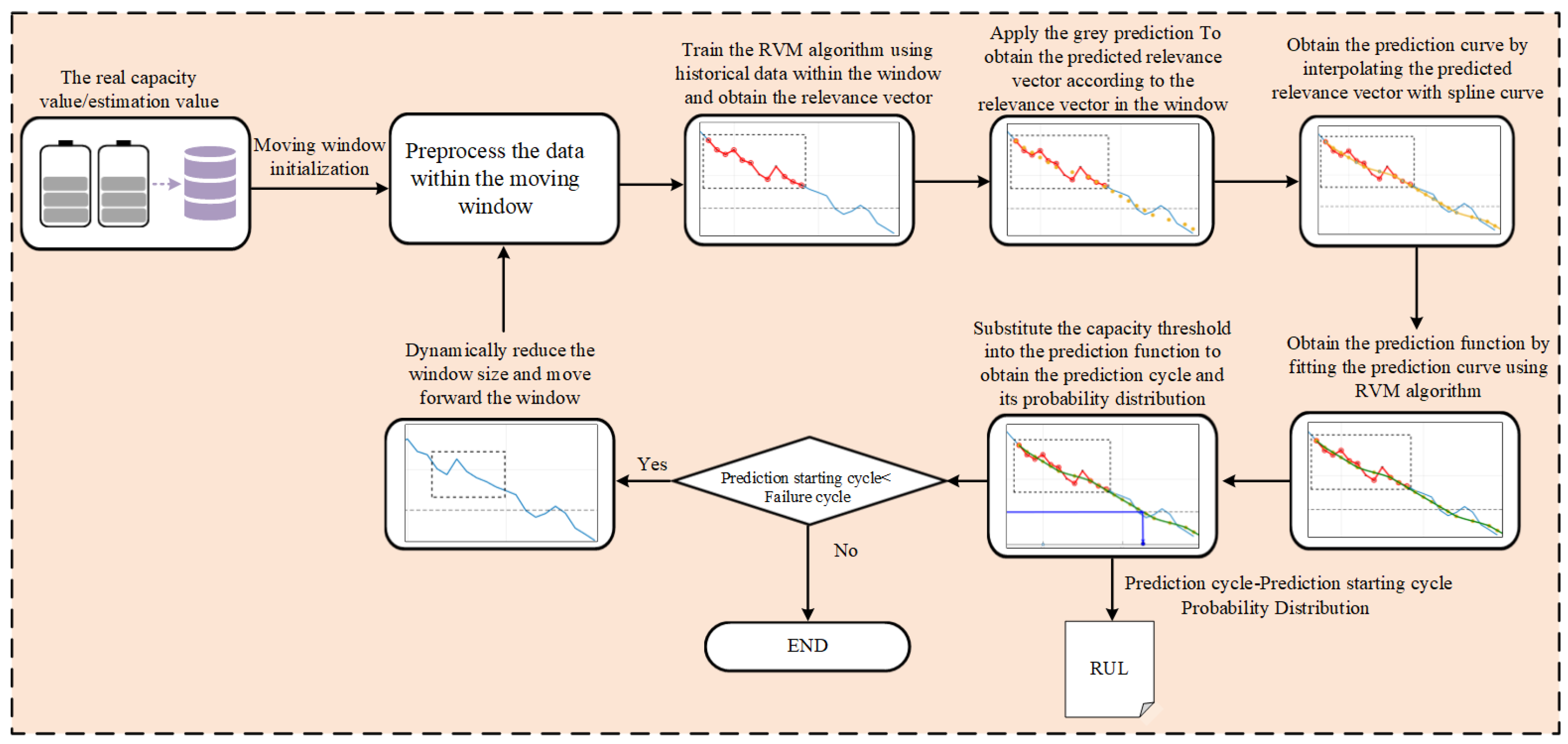
The estimated values or the actually measured capacities of lithium–ion batteries are taken as the capacity history data. The measured capacities obtained from the NASA lithium–ion battery aging experiment datasets are used to train the RVM algorithm.
(2)
Initialize the data window size and pre-process the data in the window. The window should be first initialized to select history capacity data. Then, the data in the window need to be preprocessed. If there is a large increment, the capacity sequence after this cycle shall be selected as the capacity historical data.
(3)
Train the RVM algorithm with data in the window and save the relevant vector. After preprocessing, the history capacity sequence can be input into the RVM algorithm as a training sample. The relevance vectors representing the history capacity sequence in the window can then be found.
(4)
Obtain the prediction trend of the capacity by grey prediction based on the relevance vector saved in (3). Because the capacity displays a decrement trend, the relevance vector reduction is adopted to generate grey data. The obtained predicted data point can be recognized as the relevance vector of the prediction trend curve.
(5)
Interpolate all the grey predicted points by spline curve to figure out the full prediction trend curve of the capacity. The relevance vectors in the window and the relevance vectors obtained by grey prediction form a series of characteristic discrete points representing the degradation curve. By means of spline curve interpolation, the existing discrete points are interpolated to obtain a continuous curve.
(6)
Refit the prediction trend curve to obtain the predicted function by the RVM algorithm. Combining the advantage that RVM can fit the equation and give the probability output, the curve is refitted to reach a capacity degradation trend curve equation.
(7)
Substitute the capacity failure threshold into the predicted function to obtain the predicted cycle and its probability distribution. For a certain lithium–ion battery, 80% of its nominal capacity can be regarded as the failure threshold. The threshold can be substituted into the capacity degradation trend curve equation. The predicted RUL can be expressed as N R U L = N E O L N E C L , where N R U L is the current RUL value, N E O L is the predicted cycle corresponding to the capacity degradation threshold and N E C L is the current predicted starting point.
(8)
Dynamically reduce the window size and move the window forward for circular prediction. Before the next cycle, the predicted starting point needs to be examined. If the point is smaller than the predicted failure cycle, then dynamically reduce the window size, move the window forward with a certain step length, and go back to (2) for the next prediction. Otherwise, it is considered that the point has exceeded the predicted failure cycle and the operation ends.

3. Results

In this section, the dataset of the No. 36 battery is firstly used to analyze the feasibility of the proposed RVM-GM framework. The capacity trend prediction is presented with a fixed window size. Secondly, the dynamic window sizes are introduced to make a comparison with fixed window sizes, and the datasets of No. 05, No. 32, No. 36 and No. 47 batteries are employed. Eventually, to demonstrate the effectiveness of the developed methodology, the particle filter (PF) and convolutional neural network (CNN) are chosen for comparison.

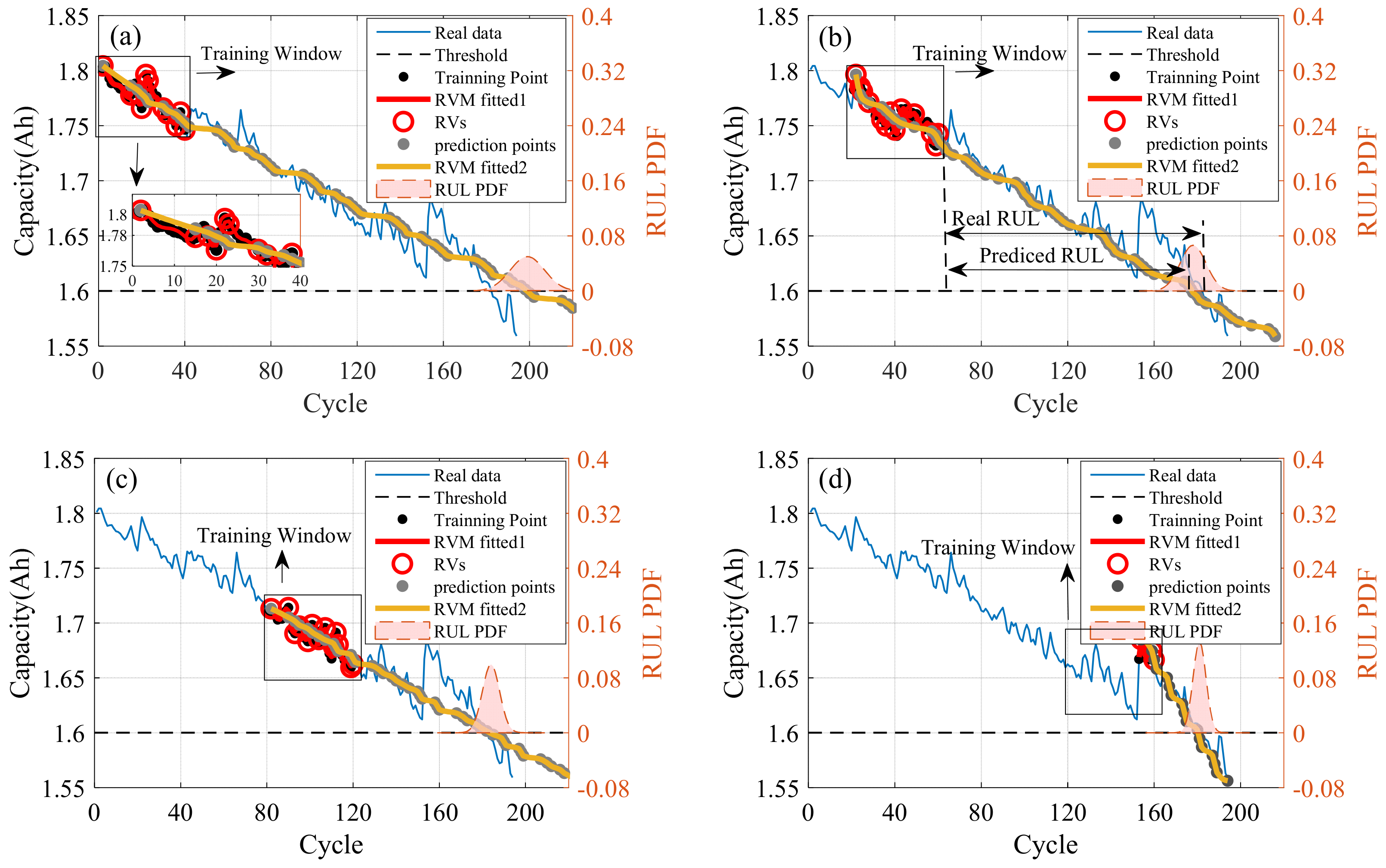
3.1. Experiment on No. 36 Battery with Window Size 40

In this case, the inspected cycles are chosen as 40, 72, 122, 162, separately. Using the proposed method with a fixed window size of 40, the RUL prediction results at each inspected cycle are plotted in Figure 2.
The red circles in the training window are the relevance vectors trained by RVM. These vectors are then used for grey prediction and function interpolation, and the prediction trend curve can be fitted as displayed by the yellow lines in Figure 2; therefore, the degradation threshold and probability distribution can be obtained by training again.
After the inspected cycle, the trend of the capacity degradation can be well tracked with the presented method. The forward movement of the window indicates the process of discarding the old capacity data timely and collecting the new capacity data simultaneously. As the window moves forward, the prediction result gets more and more accurate, and the probability density function (PDF) becomes narrower, demonstrating an increase in the confidence level of the prediction.

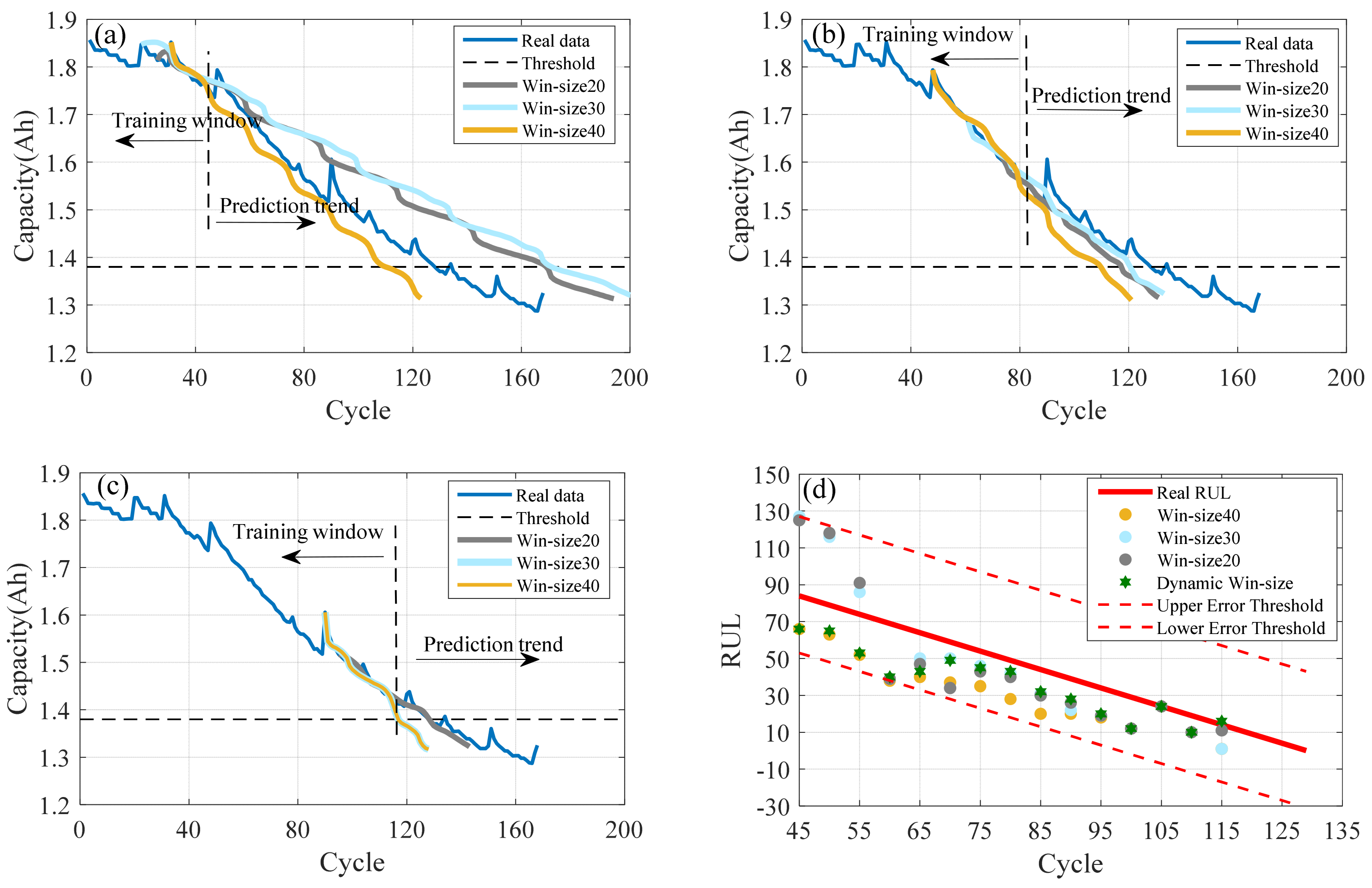
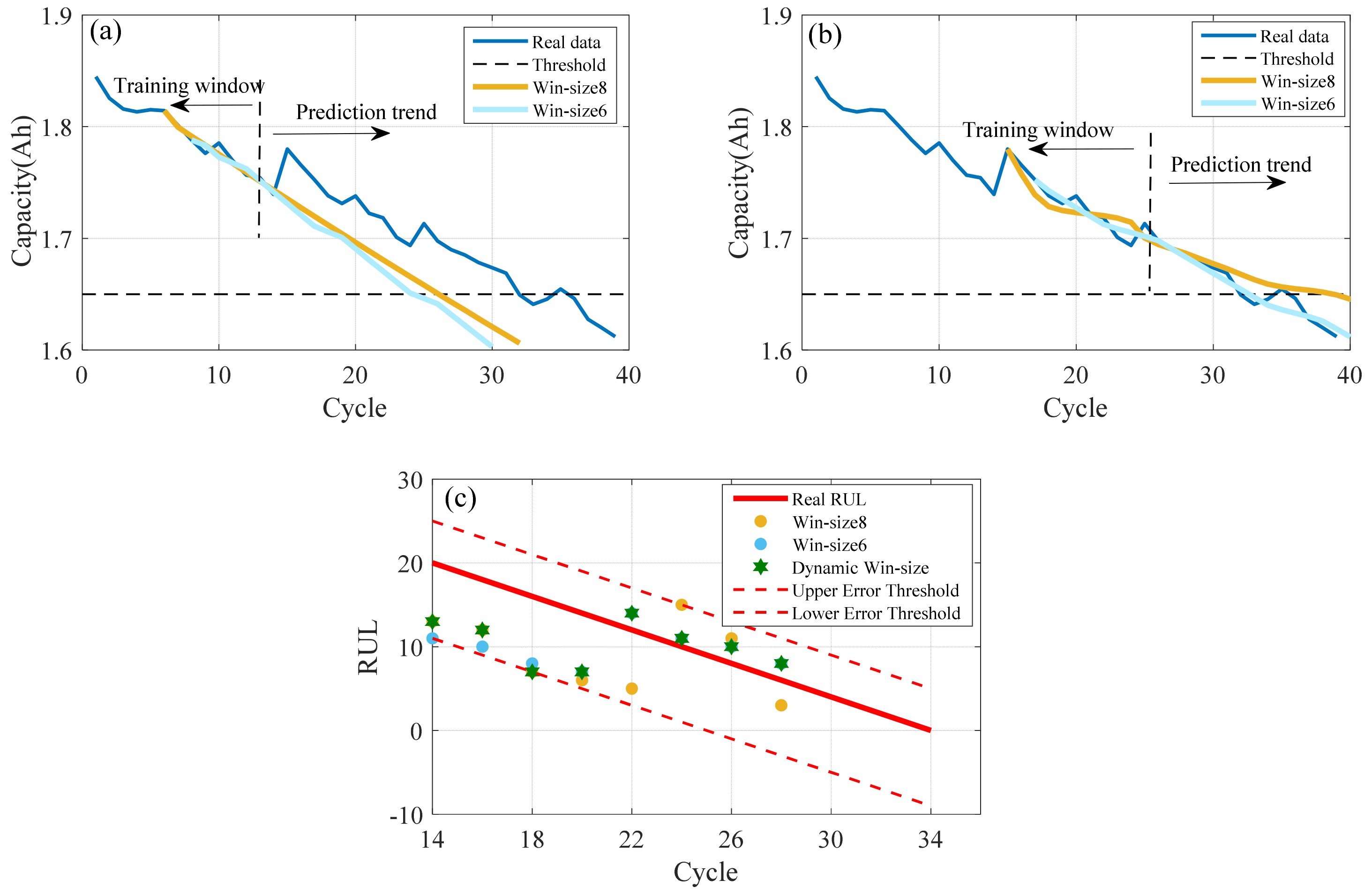
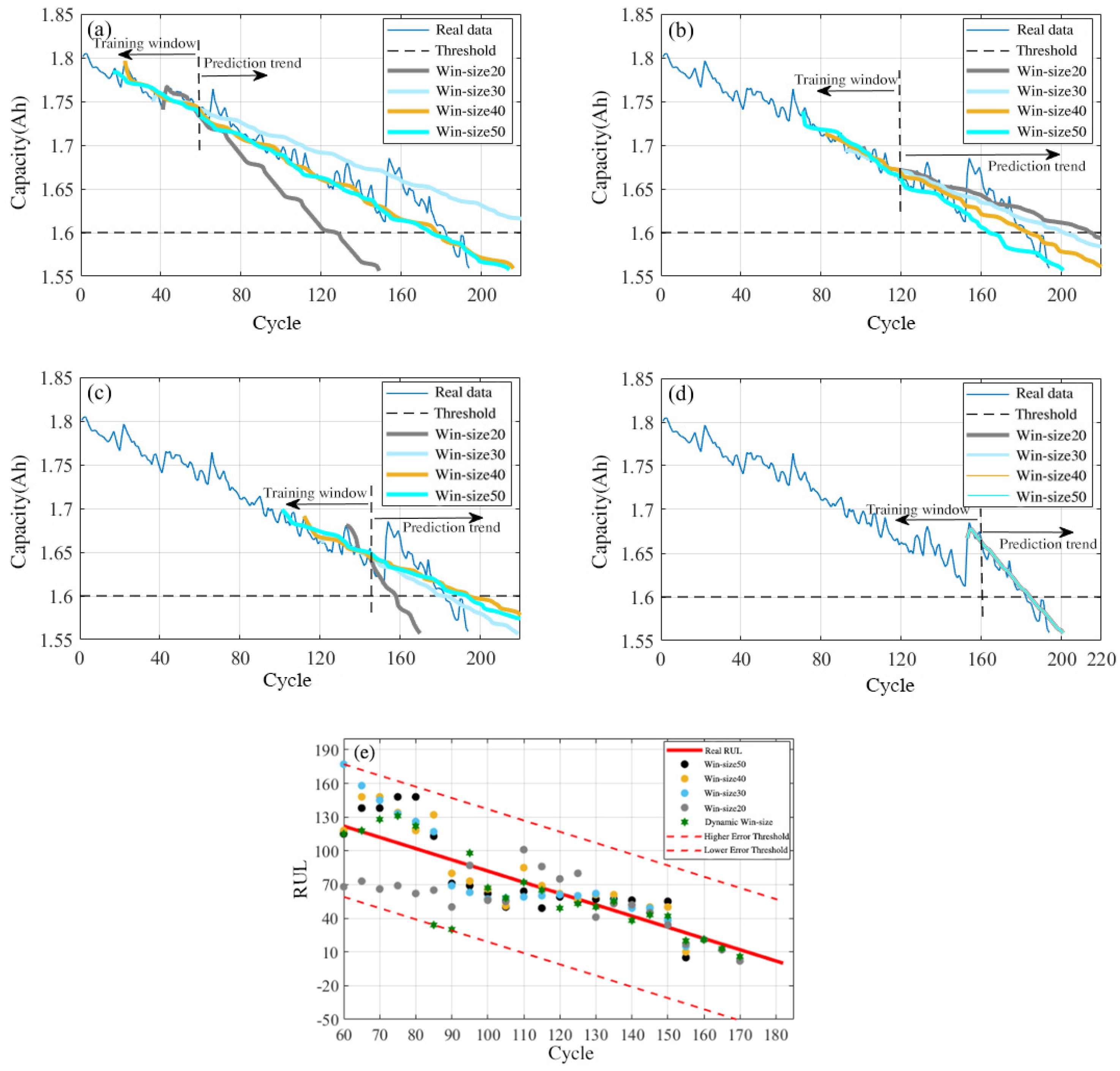
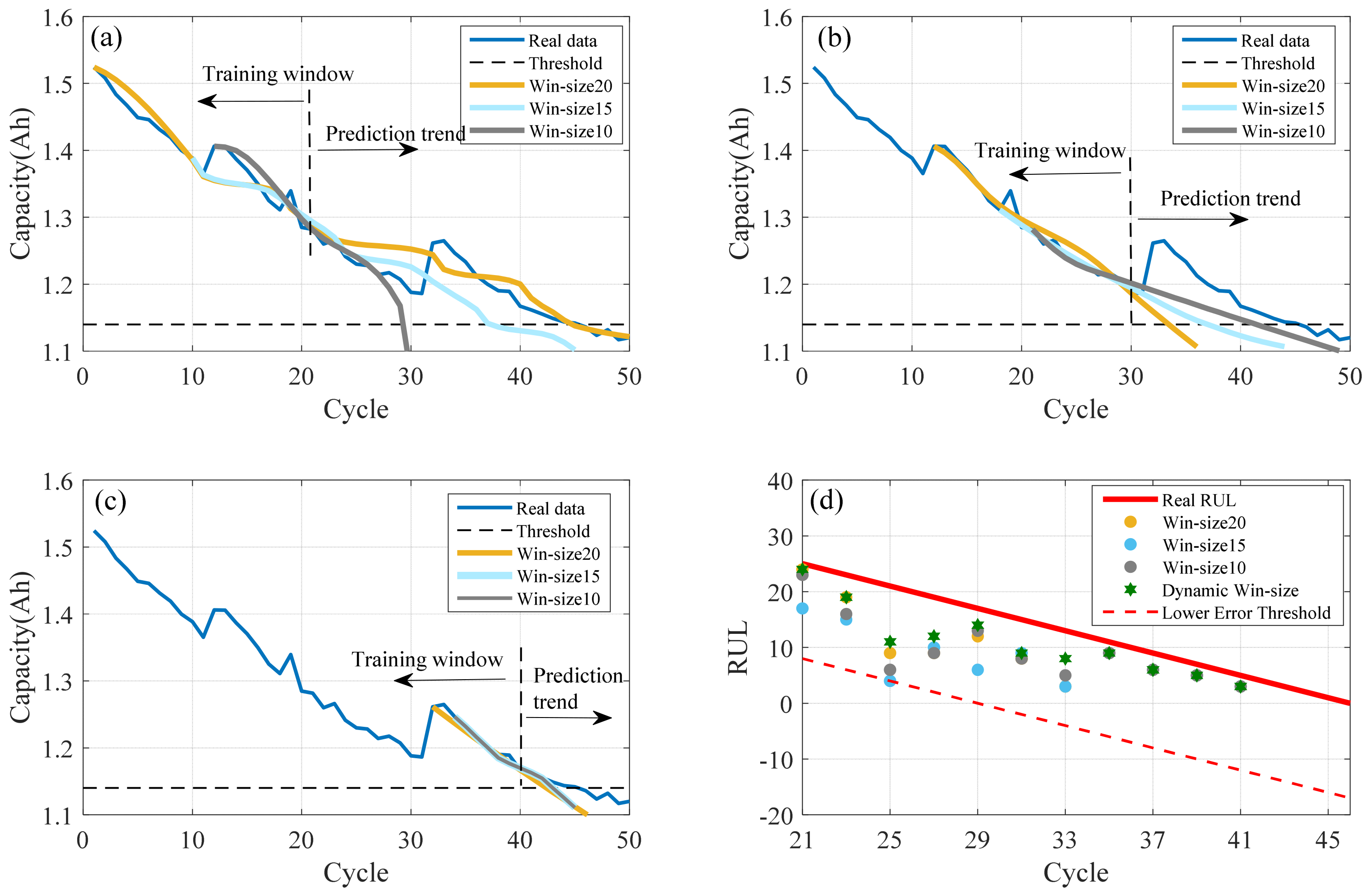
3.2. Experiment on No. 05/No. 32/No. 36/No. 47 with Dynamic Window Size

To investigate the performance of the proposed method with a dynamic size, in this case, the prediction results between different fixed window sizes and dynamic window sizes are presented. Four different operating environments of the battery datasets are considered.
Figure 3, Figure 4, Figure 5 and Figure 6 display the different prediction trends with varying sizes of moving windows, and the last sub-graphs show the error between the real RUL values and the prediction results. Further, the different statistical performance indices of RUL prediction results are compared in Table 2, including the mean absolute error (MAE), root mean squared error (RMSE), standard deviation (STD) and mean absolute percentage error (MAPE). At the same time, the detailed RUL prediction results of the selected battery datasets at several battery operation starting cycles are extended in Table A1, Table A2, Table A3 and Table A4. The prediction results, the detailed error and the 95% confidence bound of each window size and dynamic window size are listed for comparison to demonstrate the method’s accuracy. The prediction is calculated as the average result from starting cycle to the threshold. The error is computed as the difference between predicted and real RUL values. The 95% confidence bound can be expressed as the interval of the corresponding prediction.
According to the quantity of each dataset, the compared fixed window sizes are selected differently. For instance, Figure 3 illustrates the RUL prediction results of No. 05 battery with window sizes of 20, 30 and 40; however, Figure 4 depicts the results with window sizes of only 6 and 8. Figure 4c shows that even a small window can well track the trend of the lithium–ion battery capacity degradation and produce a satisfactory result.
From Figure 3, Figure 4, Figure 5 and Figure 6 and Table 2, it can be found that different fixed-size windows have different prediction results at each inspected cycle. Moreover, it can also be observed that a larger window size could generally obtain a better RUL prediction result. Interestingly, the RUL prediction using the No. 05 battery dataset with a window size of 40 is not as perfect as expected when the window moves forward, as shown in Figure 3b and Table A1. This phenomenon reveals that the larger window could not produce accurate results at particular stages; therefore, a dynamic window size is set to deal with different stages during the process of RUL prediction. As illustrated in the last sub-graphs of Figure 3, Figure 4, Figure 5 and Figure 6, the predicted values of the proposed method with a dynamic window size are generally closer to the real RUL values.
Table 2 shows that the proposed RVM-GM framework with a dynamic reducing window size outperforms the cases with fixed window sizes in terms of MAE, RMSE, STD and MAPE.

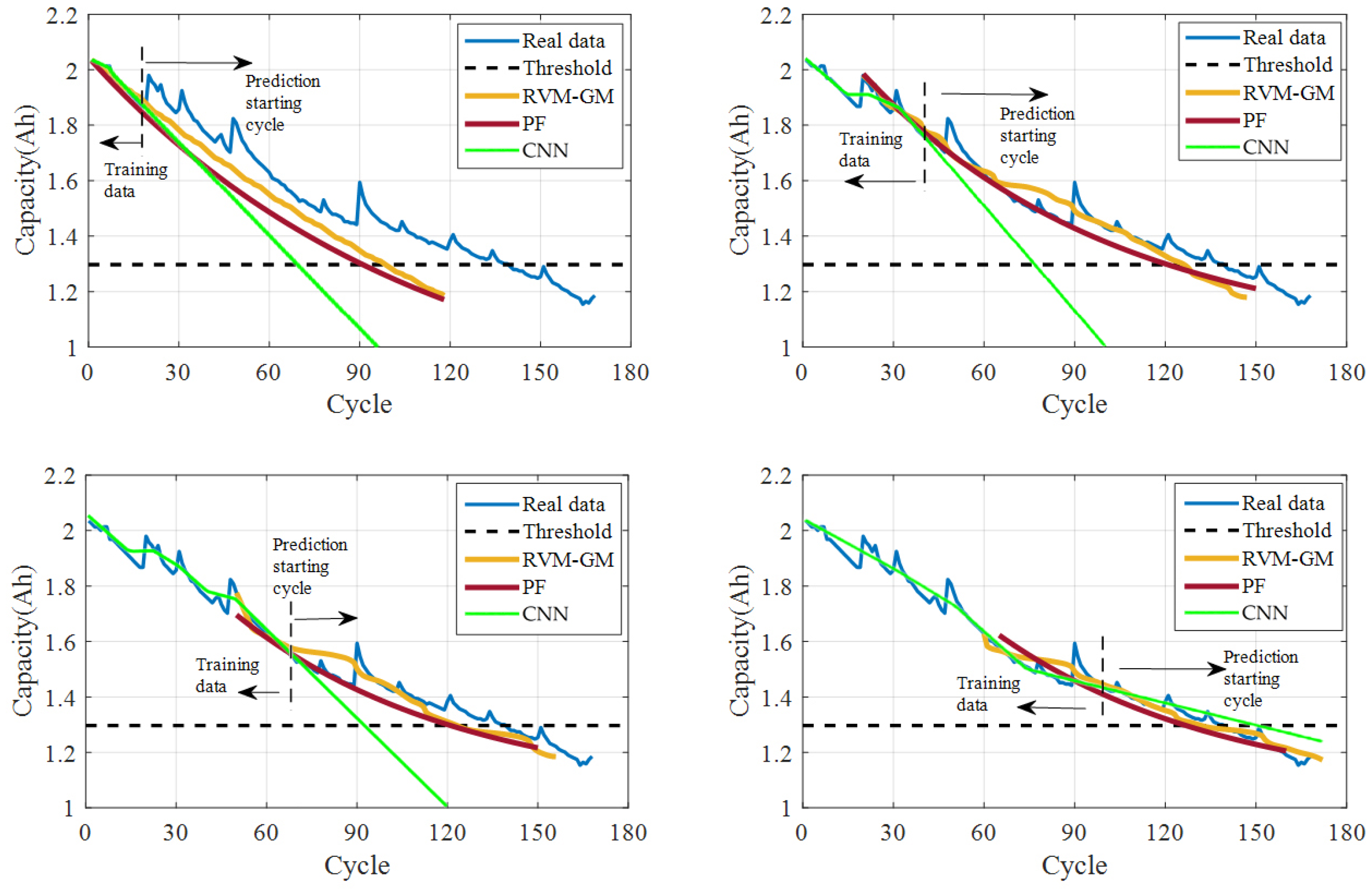
3.3. Algorithm Comparison

In this case, the particle filter (PF) and convolutional neural network (CNN) are employed for analysis. Figure 7 and Table 3 present the RUL prediction results of the proposed RVM-GM method, PF and CNN at the inspected cycles on battery No. 06. The RUL prediction error in Table 3 can be calculated as the difference between predicted and real RUL values. The 95% confidence bound is presented as the interval of RUL prediction from zero to the threshold.
It can be found in Figure 7 that the prediction curve trend of the proposed RVM-GM method with a dynamic size of moving window gets closer to the real capacity degradation trend than PF and CNN at each inspected cycle. Furthermore, the smaller RUL prediction error and the narrower PDF in Table 3 also indicate that the performed RVM-GM method with a dynamic window size can provide more accurate RUL prediction results.

4. Discussion

As described above, the experiment with a fixed window size shows that the proposed algorithm can well track the trend of the lithium–ion battery capacity degradation and results in a relatively accurate RUL prediction with only very limited data. The experiments demonstrate that different fixed-size windows have different RUL prediction results at each inspected cycle, in that the window size would affect the relevance vectors when employing the RVM, as well as affect the degradation prediction when applying GM (1,1). Further, the larger window size would generally obtain a better RUL prediction result. However, there are still some exceptions that the accuracy would not always keep in line with the changes of window size. Therefore, an appropriate window size should be set at different cycles. At the beginning of battery operating cycles, a larger window size could accept more capacity historical data, and the capacity degradation stage would be closer to the last stage. When the window moves forward, however, a smaller window size performs better at the end of the battery operating cycles, and the 95% confidence bound becomes narrower. The results indicate that the proposed RVM-GM framework with a dynamic reducing window size outperforms the cases with fixed window sizes.
Compared with the particle filter (PF) and convolutional neural network (CNN) used by most other studies, the proposed RVM-GM algorithm with dynamic window size can obtain smaller RUL prediction error and the narrower PDF, and demonstrates the effectiveness of the proposed method. Furthermore, compared with the work of [12], this paper conducts the research based on a relatively limited data and achieves satisfactory prediction results. The implementation of the dynamic window size considers the different battery capacity degradation trends at different stages in the aging process of battery compared with the work of [20].
It should be noted that this study has examined the proposed method with very limited data information. Even the RUL prediction results are satisfying; however, the accuracy of the method can be further improved by developing the proposed framework and implementing the dynamic window.

5. Conclusions

This paper presents an RVM-GM hybrid algorithm with a dynamic size of moving window to predict Li–ion battery RUL. The data-driven RVM algorithm is employed to capture the relevance vectors within the moving window, and the GM (1,1) algorithm is used to generate the prediction trends. The dynamic window size is applied to deal with the different capacity degradation trends in the battery aging process. Further, the NASA PCoE Li–ion battery data repository is utilized to assess the prediction accuracy of the proposed method. Compared with the method of fixed window sizes and mainstream RUL algorithms, the results show that the proposed method with a dynamic moving window size results in smaller RUL prediction errors and verifies the effectiveness of the proposed method. Future work will focus on more complicated battery operating conditions and try to implement the proposed method in a controller of the battery management system (BMS). Furthermore, the RVM-GM algorithm and the implementation of the dynamic window may be further optimized.

Author Contributions

Conceptualization, Z.T. and B.D.; methodology, Z.T. and B.D.; software, Z.T. and B.D.; validation, B.D., Z.T. and J.N.; formal analysis, B.D. and Z.T.; investigation, Z.T. and B.D.; resources, J.N.; data curation, Z.T. and B.D.; writing—original draft preparation, Z.T. and B.D.; writing—review and editing, B.D., W.C. and Z.T.; visualization, Z.T. and B.D.; supervision, J.N. and W.C.; funding acquisition, B.D., J.N. and W.C. All authors have read and agreed to the published version of the manuscript.

Funding

This research was funded by the National Key Research and Development Program of China, grant number 2020YFB1600203.

Data Availability Statement

Not applicable.

Conflicts of Interest

The authors declare no conflict of interest.

Appendix A

Table A1. Details of the RUL prediction results of No. 05 with different window sizes.
BatteryPredictionStarting CycleWin_Size_40Win_Size_30Win_Size_20Dynamic Win_Size
PredictionError95% Confidence BoundPredictionError95% Confidence BoundPredictionError95% Confidence BoundPredictionError95% Confidence Bound
#5456618[52, 80]12743[110, 154]12541[95, 155]6618[52, 80]
506316[47, 79]11637[95, 137]11839[99, 147]6514[50, 80]
555222[39, 65]8612[71, 101]9117[66, 116]5321[37, 69]
603831[23, 53]3930[20, 58]3930[14, 54]4029[25, 55]
654024[28, 52]5014[34, 66]4717[27, 67]4321[26, 60]
703722[23, 51]509[36, 64]3425[14, 54]4910[37, 61]
753519[24, 46]468[34, 58]4311[28, 58]459[32, 58]
802821[16, 40]427[32, 52]409[28, 52]436[33, 53]
852024[10, 30]3113[19, 43]3014[16, 44]3212[20, 44]
902019[2, 38]2217[12, 32]2613[14, 38]2811[18, 38]
951816[5, 31]1915[9, 29]1915[6, 32]2014[10, 30]
1001217[2, 32]1217[2, 22]1217[2, 22]1217[0, 24]
105240[16, 32]240[18, 30]240[19, 29]240[16, 32]
110109[4, 16]109[3, 17]109[3, 17]109[2, 18]
115113[0, 10]113[0, 12]113[6, 16]162[11, 21]
MAE 18.1 16.3 17.3 12.9
RMSE 19.3 19.8 20.8 14.8
STD 7.2 11.7 11.9 7.6
MAPE 17% 13% 14% 11%
Table A2. Details of the RUL prediction results on No. 32 with different window sizes.
BatteryPrediction Starting
Cycle
Win_Size_8Win_Size_6Dynamic Win_Size
PredictionError95% Confidence BoundPredictionError95% Confidence BoundPredictionError95% Confidence Bound
#3214137[3, 23]119[2, 20]137[3, 23]
16126[2, 22]108[2, 18]126[2, 22]
1879[1, 13]88[2, 14]79[1, 13]
2068[0, 12]77[2, 12]77[2, 12]
2257[1, 9]142[9, 19]142[9, 19]
24155[10, 25]111[7, 15]111[7, 15]
26113[8, 14]102[7, 13]102[7, 13]
2833[0, 6]82[6, 10]82[6, 10]
MAE 6.0 4.9 4.5
RMSE 6.3 5.8 5.3
STD 2.2 3.4 3.2
MAPE 21% 18% 16%
Table A3. Details of the RUL prediction results of No. 36 with different window sizes.
BatteryPrediction Starting CycleWin_Size_40Win_Size_30Win_Size_20Dynamic Win_Size
PredictionError95% Confidence BoundPredictionError95% Confidence BoundPredictionError95% Confidence BoundPredictionError95% Confidence Bound
#36601184[96, 140]17755[155, 199]6854[49, 87]1157[99, 131]
7014836[128, 168]14533[125, 165]6646[48, 84]12816[113, 143]
8011816[100, 136]12624[109, 143]6240[46, 78]12220[110, 134]
907121[58, 84]6230[49, 75]6131[46, 76]7220[62, 82]
100853[73, 97]5923[48, 70]10119[90, 112]7210[64, 80]
120611[51, 71]620[52, 72]4121[33, 49]5012[45, 55]
140508[44, 56]384[30, 46]348[29, 39]420[37, 47]
160220[0, 5]220[0, 3]220[0, 6]616[4, 7]
MAE 13.6 23.6 29.9 12.6
RMSE 17.6 28.6 33.3 14.2
STD 11.2 16.1 14.7 6.4
MAPE 7.3% 12% 21% 7.1%
Table A4. Details of RUL prediction result of No. 47 with different window sizes.
BatteryPrediction Starting
Cycle
Win_Size_20Win_Size_15Win_Size_10Dynamic Win_Size
PredictionError95% Confidence BoundPredictionError95% Confidence BoundPredictionError95% Confidence BoundPredictionError95% Confidence Bound
#4721241[20, 28]178[9, 25]232[19, 27]241[20, 28]
23194[13, 25]158[8, 22]167[8, 24]194[13, 24]
25912[4, 14]417[0, 12]615[0, 18]1110[4, 18]
27910[3, 16]109[3, 17]910[5, 13]127[6, 18]
29125[7, 17]611[0, 15]134[9, 17]143[8, 20]
3187[3, 13]96[4, 14]87[3, 13]96[4, 14]
33310[0, 11]310[0, 11]58[2, 8]85[3, 13]
3592[4, 14]92[4, 14]92[4, 14]92[4, 14]
3763[2, 10]63[2, 10]63[2, 10]63[2, 10]
3952[1, 9]52[1, 9]52[1, 9]52[1, 9]
4132[0, 6]32[0, 6]32[0, 6]32[0, 6]
MAE 5.3 7.1 5.6 4.1
RMSE 6.4 8.4 6.9 4.8
STD 3.9 4.8 4.2 2.7
MAPE 14% 20% 15% 10%

References

  1. Schmuch, R.; Wagner, R.; Hörpel, G.; Placke, T.; Winter, M. Performance and cost of materials for lithium-based rechargeable automotive batteries. Nat. Energy 2018, 3, 267–278. [Google Scholar] [CrossRef]
  2. Zhou, J.; Liu, D.; Peng, Y.; Peng, X. Dynamic battery remaining useful life estimation: An on-line data-driven approach. In Proceedings of the IEEE International Instrumentation and Measurement Technology Conference Proceedings, Graz, Austria, 13–16 May 2012; pp. 2196–2199. [Google Scholar]
  3. Zhang, Y.Z.; Xiong, R. Lithium-Ion Battery Remaining Useful Life Prediction with Box-Cox Transformation and Monte Carlo Simulation. IEEE Trans. Ind. Electron. 2019, 66, 1585–1597. [Google Scholar] [CrossRef]
  4. Chen, L.; Wang, H.; Chen, J. A novel remaining useful life prediction framework for lithium-ion battery using grey model and particle filtering. Int. J. Energy Res. 2020, 44, 7435–7449. [Google Scholar] [CrossRef]
  5. Su, X.; Wang, S.; Pecht, M. Interacting multiple model particle filter for prognostics of lithium-ion batteries. Microelectron. Reliab. 2017, 70, 59–69. [Google Scholar] [CrossRef]
  6. Jin, G.; Matthews, D.E.; Zhou, Z. A Bayesian framework for online degradation assessment and residual life prediction of secondary batteries in spacecraft. Reliab. Eng. Syst. Saf. 2013, 113, 7–20. [Google Scholar] [CrossRef]
  7. Zhang, W.G.; Shi, W.; Ma, Z.Y. Adaptive unscented Kalman filter-based state of energy and power capability estimation approach for lithium-ion battery. Power Sources 2015, 289, 50–62. [Google Scholar] [CrossRef]
  8. He, W.; Williard, N.; Chen, C.; Pecht, M. State of charge estimation for Li-ion batteries using neural network modeling and unscented Kalman filter-based error cancellation. Int. J. Electr. Power Energy Syst. 2014, 62, 783–791. [Google Scholar] [CrossRef]
  9. He, W.; Williard, N.; Osterman, M.; Pecht, M. Prognostics of lithium-ion batteries based on Dempster–Shafer theory and the Bayesian Monte Carlo method. J. Power Sources 2011, 196, 10314–10321. [Google Scholar] [CrossRef]
  10. Liu, J.; Wang, W.; Ma, F. A regularized auxiliary particle filtering approach for system state estimation and battery life prediction. Smart Mater. Struct. 2011, 20, 075021. [Google Scholar] [CrossRef]
  11. Saha, B.; Goebel, K. Modeling li-ion battery capacity depletion in a particle filtering framework. In Proceedings of the Annual Conference of the Prognostics and Health Management Society, San Diego, CA, USA, 27 September 2009; pp. 1–10. [Google Scholar]
  12. Hu, C.; Jain, G.; Tamirisa, P.; Gorka, T. Method for estimating capacity and predicting remaining useful life of lithium-ion battery. Appl. Energy 2014, 126, 182–189. [Google Scholar] [CrossRef]
  13. Sankararaman, S.; Daigle, M.; Goebel, K. Uncertainty quantification in remaining useful life prediction using first-order reliability methods. IEEE Trans. Reliab. 2014, 63, 603–619. [Google Scholar] [CrossRef]
  14. Shamshirband, S.; Fathi, M.; Dehzangi, A.; Chronopoulos, A.T.; Alinejad-Rokny, H. A review on deep learning approaches in healthcare systems: Taxonomies, challenges, and open issues. J. Biomed. Inform. 2020, 113, 103627. [Google Scholar] [CrossRef]
  15. Zhang, Y.; Xiong, R.; He, H. Long Short-Term Memory Recurrent Neural Network for Remaining Useful Life Prediction of Lithium-Ion Batteries. IEEE Trans. Veh. Technol. 2018, 67, 5695–5705. [Google Scholar] [CrossRef]
  16. Liu, J.; Saxena, A.; Goebel, K.; Saha, B.; Wang, W. An adaptive recurrent neural network for remaining useful life prediction of lithium-ion batteries. Proc. Annu. Conf. Progn. Health Manag. Soc. 2010, 2, 1–9. [Google Scholar]
  17. Liu, D.; Zhou, J.; Liao, H.; Peng, Y.; Peng, X. A health indicator extraction and optimization framework for lithium-ion battery degradation modelling and prognostics. IEEE Trans. Syst. Man. Cybern. Syst. 2015, 45, 915–928. [Google Scholar]
  18. Chinomona, B.; Chung, C.; Chang, L.K.; Su, W.C.; Tsai, M.C. Long Short-Term Memory Approach to Estimate Battery Remaining Useful Life Using Partial Data. IEEE Access 2020, 8, 165419–165431. [Google Scholar] [CrossRef]
  19. Ardeshiri, R.R.; Ma, C.B. Multivariate gated recurrent unit for battery remaining useful life prediction: A deep learning approach. Int. J. Energy Res. 2021, 45, 16633–16648. [Google Scholar] [CrossRef]
  20. Li, D.D.; Yang, L. Remaining useful life prediction of lithium battery using convolutional neural network with optimized parameters. In Proceedings of the IEEE 2020 5th Asia Conference on Power and Electrical Engineering (ACPEE), Chengdu, China, 4–7 June 2020; pp. 840–844. [Google Scholar]
  21. Li, Y.; Li, K.; Liu, X.; Wang, Y.; Zhang, L. Lithium-ion battery capacity estimation-A pruned convolutional neural network approach assisted with transfer learning. Appl. Energy 2021, 285, 116410. [Google Scholar] [CrossRef]
  22. Wilbik, A.; Kacprzyk, J. Towards a multi-criteria analysis of linguistic summaries of time series via the measure of informativeness. Int. J. Data Anal. Tech. Strateg. 2012, 4, 181–204. [Google Scholar] [CrossRef]
  23. Gupta, C.; Jain, A.; Tayal, D.K.; Castillo, O. ClusFuDE: Forecasting low dimensional numerical data using an improved method based on automatic clustering, fuzzy relationships and differential evolution. Eng. Appl. Artif. Intell. 2018, 71, 175–189. [Google Scholar] [CrossRef]
  24. Patil, M.A.; Tagade, P.; Hariharan, K.S.; Kolake, S.M.; Song, T.; Yeo, T.; Doo, S. A novel multistage support vector machine-based approach for Li ion battery remaining useful life estimation. Appl. Energy 2015, 159, 285–297. [Google Scholar] [CrossRef]
  25. Li, S. RUL prediction for lithium-ion batteries based on relevance vector machine. Comput. Eng. Des. 2018, 39, 2682–2686. (In Chinese) [Google Scholar]
  26. Liu, Y.F. A fusion prediction method of lithium-ion battery cycle-life. Chin. J. Sci. Instrum. 2015, 36, 1462–1469. (In Chinese) [Google Scholar]
  27. Zhou, J.B.; Wang, S.J.; Ma, L.P. Study on the reconfigurable remaining useful life estimation system for satellite lithium-ion battery. Chin. J. Sci. Instrum. 2013, 34, 2034–2044. (In Chinese) [Google Scholar]
  28. Wang, D.; Miao, Q.; Pecht, M. Prognostics of lithium-ion batteries based on relevance vectors and a conditional three parameter capacity degradation model. J. Power Sources 2013, 239, 253–264. [Google Scholar] [CrossRef]
  29. Gao, D.; Huang, M. Prediction of remaining useful life of lithium-ion battery based on multi-kernel support vector machine with particle swarm optimization. Power Electron. 2017, 17, 1288–1297. [Google Scholar]
  30. Liu, Y.F.; Zhao, G.Q.; Peng, X.Y. A Lithium-Ion Battery Remaining Using Life Prediction Method Based on Multi-kernel Relevance Vector Machine Optimized Model. Acta Electron. Sin. 2019, 47, 1285–1292. (In Chinese) [Google Scholar]
  31. Kheirkhah-Rad, E.; Moeini-Aghtaie, M. A novel data-driven SOH prediction model for lithium-ion batteries. In Proceedings of the 31st AUPEC, Perth, Australia, 26–30 September 2021; pp. 1–6. [Google Scholar]
  32. Tipping, M.E. Sparse Bayesian learning and the relevance vector machine. J. Mach. Learn. Res. 2001, 1, 211–244. [Google Scholar]
  33. Saha, B.; Goebel, K. Battery Data Set. In NASA Ames Prognostics Data Repository; NASA Ames Research Center: Mountain View, CA, USA, 2007. [Google Scholar]
  34. Shafiullah, M.; Abido, M.A.; Abdel-Fattah, T. Distribution Grids Fault Location employing ST based Optimized Machine Learning Approach. Energies 2018, 11, 2328. [Google Scholar] [CrossRef] [Green Version]
  35. Gilsing, R.; Turetken, O.; Ozkan, B.; Grefen, P.; Adali, O.E.; Wilbik, A.; Berkers, F. Evaluating the Design of Service-Dominant Business Models: A Qualitative Method. Pac. Asia J. Assoc. Inf. Syst. 2021, 13, 2. [Google Scholar]
  36. Zhang, H.D. EM Algorithm and Applications; Shandong University: Ji-nan, China, 2014. (In Chinese) [Google Scholar]
Figure 1. The RVM-GM algorithm for RUL prediction with dynamic size of moving window.
Wevj 13 00025 g001
Figure 2. RUL prediction result of No. 36 with a fixed window size 40: (a) inspected cycle of 40; (b) inspected cycle of 72; (c) inspected cycle of 122; (d) inspected cycle of 162.
Wevj 13 00025 g002
Figure 3. RUL prediction results of No. 05 with a dynamic window size: (a) prediction starting cycle of 42; (b) prediction starting cycle of 82; (c) prediction starting cycle of 118; (d) RUL prediction results.
Wevj 13 00025 g003
Figure 4. RUL prediction results of No. 32 with a dynamic window size: (a) prediction starting cycle of 13; (b) prediction starting cycle of 25; (c) RUL prediction results.
Wevj 13 00025 g004
Figure 5. RUL prediction results of No. 36 with a dynamic window size: (a) starting cycle of 60; (b) starting cycle of 120; (c) starting cycle of 150; (d) starting cycle of 160; (e) RUL prediction results.
Wevj 13 00025 g005
Figure 6. RUL prediction results of No. 47 with a dynamic window size: (a) prediction starting cycle of 21; (b) prediction starting cycle of 30; (c) prediction starting cycle of 40; (d) RUL prediction results.
Wevj 13 00025 g006
Figure 7. RUL prediction results between RVM-GM, PF and CNN algorithm.
Wevj 13 00025 g007
Table 1. This List of batteries with their operating parameters.
Battery NumberDischarge CurrentEnd Voltage(V)Charge CurrentEnd-of-Life
(Capacity Fade (%))
Operating Temperature (°C)Number of Cycles
No. 052A constant current2.71.5CC mode then change to 4.2V CV mode 30%24168
No. 062A constant current2.530%24168
No. 324A constant current2.720%4340
No. 362A constant current2.720%24197
No. 47Fixed loaded-1A2.530%472
Table 2. Prediction results of four types of batteries under different experimental conditions.
BatteryWindow SizeMAERMSESTDMAPE
No. 05Dynamic12.914.87.611.5%
2017.320.811.913.8%
3016.319.811.712.8%
4018.119.37.216.7%
No. 32Dynamic4.55.33.216.1%
64.95.83.417.9%
86.06.32.221.3%
No. 36Dynamic12.614.26.47.1%
2029.933.314.720.5%
3023.628.616.112.4%
4013.617.611.27.3%
No. 47Dynamic4.14.82.710.2%
105.66.94.215.3%
157.18.44.820.0%
205.36.43.913.9%
Table 3. RUL prediction results for comparison.
AlgorithmPrediction Starting CycleRUL Prediction Error95% Confidence Bound
RVM-GM1540[89, 111]
4017[116, 130]
7019[115, 127]
10015[121, 128]
PF1549[78, 103]
4023[105, 128]
7021[108, 129]
10019[115, 127]
CNN1571[68, 70]
4055[73, 96]
7045[86, 104]
10021[153, 168]
Publisher’s Note: MDPI stays neutral with regard to jurisdictional claims in published maps and institutional affiliations.

