Obstacle-Avoidance Path-Planning Algorithm for Autonomous Vehicles Based on B-Spline Algorithm

Abstract

To solve the problem of the real-time path-planning of autonomous vehicles for obstacle avoidance on structured roads, a path-planning approach based on the B-spline algorithm is proposed in this paper. Firstly, the mechanism of driver path planning is analyzed, and a dynamic risk-identification model based on the support vector machine is proposed. It combines the driver’s risk perception characteristics and a risk model. Then, the B-spline algorithm model is improved based on the risk-identification model. Furthermore, road features, road constraints and dynamic constraints are considered to further optimize the planning algorithm. To verify the path-planning approach proposed in this paper, a co-simulation experiment based on CarSim/Simulink is conducted. Results show that the improved algorithm is effective in static and dynamic obstacles avoidance. The algorithm can generate collision-free obstacle avoidance paths, and the paths meet the real-time requirements and dynamic constraints of obstacle avoidance scenarios. In addition, the proposed algorithm optimizes the path according to the driver’s operating characteristics, which can further improve the safety and comfort of autonomous vehicles.

1. Introduction

Autonomous vehicles can reduce traffic accidents, improve traffic efficiency, reduce the operating burden of drivers and effectively improve the overall security of the traffic system [1,2]. In recent years, the research on the technologies related to autonomous vehicles has received extensive attention and concern. Before realizing autonomous driving, we still need to solve the key problems, including real-time dynamic environment perception, complex decision making, dynamic path planning and so on [3,4,5]. Dynamic path planning needs to combine real-time environmental information to plan a real-time, reasonable and collision-free path. It is the key technology for the safe driving of autonomous vehicles. Many scholars have carried out a lot of research on dynamic path planning.

Path planning finds the available trajectory for an autonomous vehicle in an environment with obstacles, so that they can be avoided. Dynamic obstacle-avoidance path planning has the characteristics of time-varying and highly dynamic scenes, which makes it difficult to design an algorithm with real-time capabilities; it is easy for solutions to fall into local optima [6,7]. The current path-planning algorithms cannot meet all the working conditions needed and cannot ensure the optimal path selection. There is a certain tension between the real-time performance of the algorithm and the planning performance [8,9]. In the research of local path planning for autonomous vehicles, how to use an appropriate planning algorithm according to the information while taking into account the search efficiency, and how to establish a relatively perfect path-planning model for obstacle-avoidance path planning and path optimization for autonomous vehicles in a dynamic environment have become new research hot spots. Common methods for vehicle obstacle avoidance path planning include the intelligent water drop algorithm, the grid method, the artificial potential field method, the rapidly exploring random tree (RRT) algorithm and the probabilistic road maps (PRM) algorithm. Ji et al. used the trapezoidal acceleration method to design the virtual ideal trajectories in lane changes, solved the relationship between the change rate of lateral acceleration and the lane change time and solved the planning problem of finding a lane-change path in a setting with known road parameters [10]. In order to improve the safety of obstacle-avoidance path planning, Luo converted the planning problem into a constrained optimization problem by using the time and distance involved in a lane change and designed a trajectory-function planning method based on a quantization polynomial [11]. This method can update the reference trajectory during lane change to avoid potential collisions. Chen proposed a low-speed obstacle-avoidance path-planning method for autonomous vehicles based on the polar coordinate algorithm [12]. This algorithm has high adaptability in complex scenes, and the real-time performance and application performance of the algorithm still need to be improved. Wang fused the vehicles parameters and the driver’s intention to quickly evaluate the risk level faced by vehicles during driving, and generated a smooth, safe collision-avoidance trajectory based on the improved fast exploration random tree algorithm according to the risk level [13].

Considering the requirements of safety and real-time performance in dynamic traffic scenario, an obstacle-avoidance path-planning algorithm based on B-spline curves for autonomous vehicles is proposed in this paper. The main contributions of this paper are as follows: firstly, the mechanism of driver path planning is analyzed, and a dynamic risk-identification model based on the support vector machine is proposed. It combines the driver’s risk perception characteristics and a risk model. Then, the B-spline algorithm model is improved based on the risk-identification model. Furthermore, road features, road constraints and dynamic constraints are considered to further optimize the planning algorithm.

2. Risk-Identification Model Based on SVM

According to research by the national highway traffic safety administration (NHTSA), nearly 30% of traffic accidents occur during lane changes [14]. In a dynamic traffic scenario, vehicles can avoid obstacles by changing lanes. Therefore, the establishment of a quantitative model of lane-changing risk has great influence in the path-planning algorithm design. In order to reduce the property loss and personal injuries caused by traffic accidents, researchers have classified the possible accidents during lane change and established risk-identification models [15]. The results showed that the severity of a collision during a lane change is related to the speed, motion state and physical characteristics of the obstacle. Therefore, combining the characteristics of the obstacle with the psychological characteristics and operational characteristics of drivers, the researchers believe that performing the obstacle avoidance operation 0.3 to 1 s in advance would effectively improve the safety of the obstacle-avoidance process [16]. On this basis, a simplified obstacle-avoidance safety model was established by combining the above driving-risk model and driver-behavior characteristics. By analyzing the obstacle-avoidance-operation characteristics of human drivers, it can be seen that the parameters of the obstacle ahead, including the size, type, weight and other factors, have a great impact on the driver’s lane-change decision. When the mass and volume of the obstacles are large, the driver thinks that the risk index of the current lane is high and tends to avoid the obstacle in advance. In addition, when the width of obstacles is large or the obstacle shows a trend of lateral movement, besides changing lane in advance, drivers usually keep larger lateral distance from obstacles to ensure the safety of the ego vehicle.

In actual driving process, the obstacle avoidance strategies of static obstacles and dynamic obstacles are different. Due to the uncertainty of dynamic obstacles, the design of obstacle avoidance strategies and path-planning algorithms is more complex. Therefore, the generated paths of autonomous vehicle obstacle avoidance should not only be collision free; they should also optimize the generated paths with real-time scenario information, which can further improve the availability and safety of generated paths. Human drivers will plan and choose different obstacle avoidance paths through different types of obstacles. One of the key factors of the driver path-planning strategy is to evaluate the ego vehicle collision damage degrees with different obstacles [17]. The collision loss function describes the loss caused by collision between an ego-vehicle and obstacles when collision is unavoidable. The data show that the collision loss is related to the attributes of the collision object. The damage degree of ego-vehicle increases with the obstacle mass in collision. Therefore, the mass ratio of obstacle and ego-vehicle can be used to describe the impact of mass on collision loss. In addition, higher relative speed will also cause greater collision losses. Similarly, the speed ratio of the obstacle and the ego-vehicle can be used to describe the impact of speed on collision loss. Furthermore, the distance between the obstacle and ego-vehicle should also be considered, and the distance ratio is also used to describe collision losses. Based on the above analysis, the collision loss equation between ego-vehicle and obstacle can be expressed as [17]:

$$L_i{=f(m}_i{/m,T}_i,\mathsf{\Delta }{v}_i{,s}_i{)=T}_i\left(\frac{m_i}{m}+\frac{\mathsf{\Delta }{v}_i}{\mathsf{\Delta }{v}_0}+\frac{d_e{-s}_i}{d_e}\right),$$

(1)

where $\mathsf{\Delta }{v}_0$ is the speed difference between the vehicle and the object i. In the determination of type T_i value, the standard value can be set to one. For other types of objects, the T value is the ratio of the average loss of this type of object to the average loss of the standard type. When collisions are unavoidable, the types of obstacles that collide with autonomous vehicles can be generally divided into three types [17]. Additionally, according to the types, the risky level can be divided into three levels.

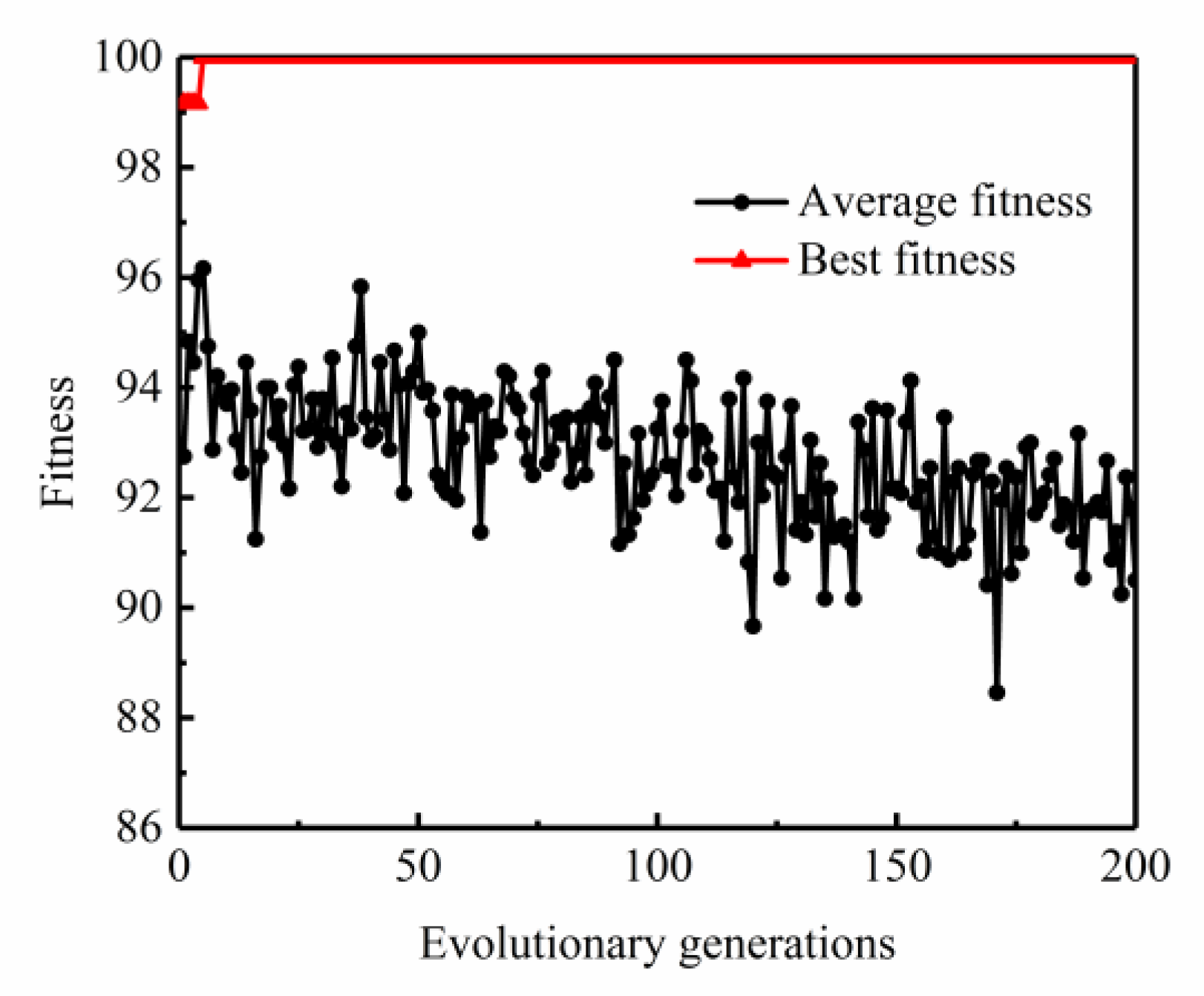
Based on the above collision loss model, the risk level of obstacles ahead is related to their shape, weight and relative speed. In order to complete the dynamic risk assessment of autonomous vehicles, according to the above risk assessment model, an obstacle risk identification model based on support vector machine (SVM) is proposed. The model is trained with the NGSIM dataset. Various traffic state databases such as vehicle category, size, position, speed, acceleration, space headway, time headway and relationship with surrounding vehicles in the dataset are set as the input of the model. In order to obtain the optimal results, particle swarm optimization (PSO) algorithm is used to optimize the SVM model. The penalty coefficient C and the Gaussian kernel parameter g with the highest classification accuracy are selected. The optimization process is shown in Figure 1.

To verify the performance of the constructed PSO-SVM model, the test datasets are imported for classification verification. The results are shown in Figure 2. Through comparison with the actual results in the test set, the PSO-SVM model can correctly identify the samples in the test set and complete the identification of the types and the risk identification of obstacles.

3. B-Spline Algorithm

The B-spline curve was proposed by Schoen-berg in the 1940s [18]. The algorithm generates a curve shape by combining control points with B-spline basis functions. A cubic quasi-uniform B-spline curve is used for path planning in this paper. As the repeatability of the panel point at both ends is k, the curve starts at the first control point and ends at the last control point. In the path-planning algorithm design process, the requirements of remaining collision free and vehicle dynamics constraints should be meet. Then, the control points are selected according to the above constraints. In order to obtain obstacle avoidance paths meeting the application conditions, the selected control points are fused with the B-spline basis function and safety model. The specific relationship among curves, control points and B-spline basis functions is as follows, where P_i (i = 0, 1, 2, …, n) is the control point, and n + 1 control points are fused with B-spline curve baseline. The k-order B-spline is:

$$P\left(t\right)=\left[P_0{P}_1{P}_2\dots P_n\right]\left[\begin{array}{c}{B}_{0,k}\left(t\right)\\ B_{1,k}\left(t\right)\\ B_{2,k}\left(t\right)\\ ⋮\\ B_{n,k}\left(t\right)\end{array}\right]={{\displaystyle \sum }}_{i=0}^n{P}_i{B}_{i,k}\left(t\right),$$

(2)

where $B_{i,k}\left(t\right)$ represents the B-spline basis function of the ith order k at point t, t is the position independent variable, k is the degree of the basis function and $t\in [0,1]$.

The recurrence formula of B-spline basis function is expressed as follows:

$$B_{i,k}\left(t\right)=\frac{1}{k\mathit{!}}{\left(-1\right)}^j{C}_{k+1}^j{\left(t+k-i-j\right)}^k,$$

(3)

where i = 0, 1, 2, …, k − 1; $C_{k+1}^j=\frac{\left(n+1\right)\mathit{!}}{j\mathit{!}\left(n+1-j\right)}$.

Based on the above two formulas, it can be seen that the spline curve is generated by weighting the control points according to the spline basis function. The shape of the curve can be adjusted by changing the position of the spline control point, and it can synthesize the optimization results and computational complexity. A cubic quasi-uniform B-spline curve is applied to complete path planning in this paper, then:

$$P\left(t\right)={{\displaystyle \sum }}_{i=0}^3{P}_i{B}_{i,3}\left(t\right),$$

(4)

According to the spline basis function, the cubic B-spline curve can be expressed as:

$$P\left(t\right)=\frac{1}{6}{\left[\begin{array}{c}{t}^0\\ t^1\\ t^2\\ t^3\end{array}\right]}^T\left[\begin{array}{cccc}1& 4& 1& 0\\ -3& 0& 3& 0\\ 3& -6& 3& 0\\ -1& 3& -3& 1\end{array}\right]\left[\begin{array}{c}{P}_0\\ P_1\\ P_2\\ P_3\end{array}\right],$$

(5)

where $P_i$ is the control point and $P_0$ is the starting point, take four points as control points to get the first cubic B-spline curve. Then, starting with $P_1$, draw the second curve with the following four control points. The second derivative between curves is continuous.

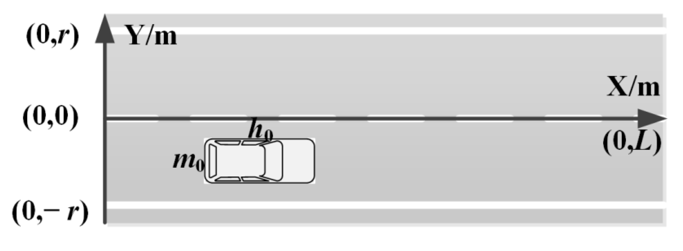
The local obstacle avoidance path-planning process of autonomous vehicles is composed of obstacle detection, information processing and obstacle avoidance path generation. The autonomous vehicle obtains environment information and vehicle state information through on-board sensors. Based on the environment information and vehicle state information, the obstacle avoidance system of autonomous vehicle analyzes the real-time potential risk, and then the optimal obstacle avoidance path is generated. Additionally, the autonomous vehicle returns to the original lane after obstacle avoidance. The road model is established as shown in Figure 3. The length and width of the vehicle are h₀ and m₀, respectively. The length of the road is L and the width is 2r. During normal driving, the vehicle body shall be in the lane, and it will not cross the road boundary except during lane changes. Then, the selection range of B-spline control point position (x, y) is:

$$\left\{\begin{array}{c}{h}_0<x<L\\ \frac{m_0}{2}-r<y<r-\frac{m_0}{2}\end{array}\right.,$$

(6)

Local obstacle avoidance path planning is implemented based on global path. When an obstacle appears on the global reference path, the local obstacle avoidance path is planned according to the vehicle information and the surrounding environment information to correct the vehicle driving reference path. When there are obstacles in the original path, autonomous vehicle needs to implement local path planning based on the global path and real-time environment information. The cubic quasi-uniform B-spline algorithm can ensure the smoothness of the generated path, while the parameters of control points have a great impact on path availability. Therefore, in order to further ensure the availability of the generated path, the selection of control points of B-spline algorithm is improved in combination with obstacle avoidance scenarios in this paper. In the process of obstacle avoidance, autonomous vehicles cross lane lines to the target lane. The collision probability during lane change is greater than the other stage. Therefore, it is necessary to analyze the obstacle avoidance process and establish an obstacle avoidance safety model.

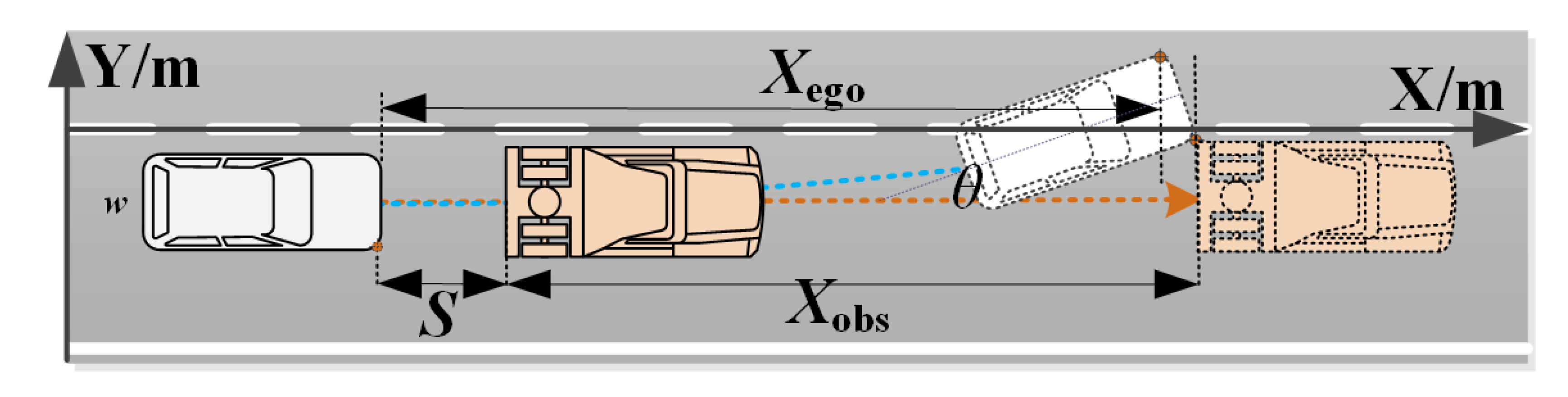
In the process of obstacle avoidance, the conditions under which the ego-vehicle does not collide with the moving obstacle in front can be expressed as:

$$X_{\mathit{ego}}{+\mathit{w}\sin \theta <X}_{\mathit{obs}}+S,$$

(7)

where $X_{\mathit{ego}}$ indicates the longitudinal displacement of the ego-vehicle during the obstacle avoidance process shown in Figure 4; $X_{\mathit{obs}}$ indicates the longitudinal displacement of the obstacle vehicle in the process of obstacle avoidance; $S$ indicates the initial distance between the own vehicle and the obstacle vehicle; $w$ indicates the width of the ego-vehicle; $\theta$ indicates the included angle between the X axis of the vehicle coordinate system and the lane; the value of $\theta$ is related to the lateral speed of the vehicle.

It can be seen in Figure 4 that the longitudinal displacement generated by the ego-vehicle during the obstacle avoidance process can be expressed by the following formula:

$$X_{\mathit{ego}}={{\displaystyle \int }}_0^{t_c}\dot{X_{\mathit{ego}}}\mathrm{dt},$$

(8)

Similarly, the longitudinal displacement of the obstacle vehicle during the obstacle avoidance process shown in Figure 4 can be expressed by the following formula:

$$X_{\mathit{obs}}={{\displaystyle \int }}_0^{t_c}\dot{X_{\mathit{obs}}}\mathrm{dt},$$

(9)

where $t_c$ is the time period in which the ego-vehicle starts decelerate and reach the critical point of collision. In order to ensure that there is no collision within the time period of obstacle avoidance shown in Figure 4, it can be inferred from formula (7) that the initial distance S should meet the following conditions:

$${S=X}_{\mathit{ego}}+w\sin \theta -X_{\mathit{obs}}>0,$$

(10)

Combining the above formula with the vehicle kinematics model in the obstacle avoidance process shown in Figure 4, the minimum longitudinal safety distance required for the ego-vehicle to complete the obstacle avoidance without collision can be expressed as:

$$\min S=\left(\dot{X_{\mathit{ego}}}\dot{-X_{\mathit{obs}}}\right)t_c+{{\displaystyle \int }}_0^{t_{\mathrm{c}}}{{\displaystyle \int }}_0^{\mathsf{\delta }}\left(\ddot{X_{\mathit{ego}}}\left(t\right)-\ddot{X_{\mathit{obs}}}\left(t\right)\right)d_{\mathsf{\delta }}d{t}_c+w\sin \theta ,$$

(11)

Autonomous vehicle obstacle avoidance and lane changes take a short time in real traffic scenarios. The following assumptions can be made: the ego-vehicle braking deceleration is constant and the speed of the obstacle is stable. The time taken for the ego-vehicle to decelerate to the same speed as the obstacle vehicle can be regarded as the critical time of collision.

In a real traffic scenario, the relative speed of the vehicle is usually low when it overtakes an obstacle vehicle, resulting in errors in the calculation results of formula (11). In order to ensure driving safety, this paper improves the minimum safe distance model in formula (11) by considering the headway and driver behavior characteristics, and the improved model can be expressed as:

$$\min D=\min S+c\left(\dot{X_{\mathrm{ego}}}\dot{-X_{\mathit{obs}}}\right){+d}_0+\sigma \left(\dot{X_{\mathit{ego}}}\dot{-X_{\mathit{obs}}}\right),$$

(12)

where c represents the headway, $d_0$ represents the safety breaking distance threshold, $\sigma$ is the hazard characterization coefficient of obstacles, which $\sigma \in [1,1.5]$.

By considering the drivers’ operation characteristics and combining the real-time obstacle information, the original minimum longitudinal safe distance is improved. The improved safety model can adjust the selection of safety margin in different scenarios according to the type and moving state of obstacles. This improvement can optimize the path-planning algorithm, further improve the safety of the generated paths and ensure the safety of autonomous vehicle obstacle avoidance.

The control points position of the B-spline algorithm should be determined according to the real-time position of obstacles on the road. The rear center point of the obstacle vehicle is selected as (x₀, −$\frac{r}{2}$), and the first control point is set as P₀ = (x₀ − minD, −$\frac{r}{2}$). Meanwhile, in order to satisfy that the yaw of autonomous vehicle at the initial time is zero without sudden change, set P₂ = (x₀ + h₀ − minD, −$\frac{r}{2}$). To further strengthen this constraint, set the control point P₁ = (x₀$+\frac{h_0}{2}$ − minD, −$\frac{r}{2}$). Assuming that the vehicle is driving at the original speed, when the distance from the obstacle vehicle to the collision-free critical position is minD. At this time, the displacement of the obstacle vehicle can be expressed as:

$$x_1=\dot{X_{\mathit{obs}}}\times \frac{\mathit{minD}}{\dot{X_{\mathit{ego}}}\dot{-X_{\mathit{obs}}}},$$

(13)

Therefore, when the obstacle vehicle reaches the critical position, its rear abscissa is x₀ + x₁. If the head abscissa of the autonomous vehicle is located at x₀ + x₁, the vehicle can cross the lane line to the target lane. This ensures that the ego-vehicle has enough safety space from the obstacle vehicle and the roadside. In addition, the lateral displacement of the ego-vehicle is small in this period, which ensures that the lateral acceleration takes place within a reasonable range. Therefore, the control point is P₃ = (x₀ + x₁, $\frac{r}{2}$).

After entering the target lane, the autonomous vehicle will drive along the center of the target lane. When the ego-vehicle finishes overtaking and reaches a safe distance from the obstacle vehicle, the ego-vehicle will return to the original lane. The time required for the autonomous vehicle to complete the above operations can be expressed as:

$$t=\frac{{\mathit{2}h}_0{+h}_1}{\dot{X_{\mathit{ego}}}\dot{-X_{\mathit{obs}}}},$$

(14)

where h₀ is the length of the ego-vehicle; h₁ is the length of the obstacle vehicle.

Therefore, the starting abscissa of autonomous driving back to the original lane can be expressed as:

$$x_2=x_0{+x}_1+\dot{X_{\mathit{obs}}}{t+h}_0,$$

(15)

Then, the control point $P$₄ = ($x$₀ +$x$₁$+\frac{X_{\mathrm{obs}}^{’}t}{2}{+h}_0$, $\frac{r}{2}$), $P$₅ = ($x$₂, $\frac{r}{2}$) is selected. The path back to the original lane is set to be symmetrical with the obstacle avoidance path. Additionally, the control point $P$₆ = (minD + $x$₂ − $h$₀, −$\frac{r}{2}$), $P$₇ = (min$D+x$₂ − $\frac{h_0}{2}$, −$\frac{r}{2}$), P₈ = (minD$+$x₂, −$\frac{r}{2}$) is selected, respectively.

4. Simulation Analysis

In order to verify the availability of the proposed planning algorithm in this paper, a series of simulation experiments are carried out. To fully verify the planning performance of the algorithm, static and dynamic obstacles are set for simulation testing in the dynamic traffic scenario.

The simulation results of autonomous vehicle avoiding static obstacles are shown in Figure 5 and Figure 6. The results show that the proposed algorithm can generate available paths for autonomous vehicle in dynamic traffic scenarios. The vehicle can track the path to bypass the static obstacles. Additionally, the risk-identification model proposed in this paper can complete the risk assessment of obstacles according to different obstacles. Additionally, the algorithm can generate different obstacle avoidance paths according to the real-time risk assessment results. For obstacles with higher risk level, the generated path has a higher safety margin. In addition, a large safety margin will be reserved when the relative speed between the ego-vehicle and the obstacle is large. The path planned by the algorithm proposed in this paper is more consistent with the operation habits of human drivers, which can further ensure vehicle safety and improve ride comfort.

The simulation results of vehicles avoiding dynamic obstacles are shown in Figure 7 and Figure 8. The results show that the proposed algorithm can generate available paths for autonomous vehicles in a dynamic traffic scenario with moving obstacles. When the speed of the obstacle vehicle is 10 km/h and the speed of the ego-vehicle is 35 km/h and 70 km/h, respectively, the algorithms in the above scenarios can generate reasonable real-time obstacle avoidance paths. The vehicle can track the path to bypass the moving obstacles. Furthermore, the risk-identification model proposed in this paper can complete the risk assessment of moving obstacles according to different moving states. Collision-free paths can be real-time generated for different types of vehicles in dynamic scenarios. A large safety margin will be reserved when the size of moving obstacle vehicles is large, which further ensures the safety performance of the generated paths. In addition, the generated paths also conform to the boundary constraints of the structured road, which can keep the ego-vehicle driving in the center of the structured road lane.

5. Path Tracking Method Based on LQR

The path-planning algorithm for autonomous vehicles should not only meet the requirements of a collision-free path, but also meets the requirements of path smoothness. The generated paths are smooth and can be tracked by autonomous vehicles. The generated path should conform to the dynamic constraints of the vehicle. Therefore, it is necessary to further verify the availability of the generation paths. The effectiveness of the path generated by the obstacle avoidance path algorithm can be fully verified through real vehicle experiments. However, due to the high cost of real vehicle experiments and the risk of real vehicle high-speed path tracking experiments, most path availability experiments are currently completed through Co-simulation experiments.

In order to verify the path availability, a path tracking model based on a Linear Quadratic Regulator (LQR) approach for autonomous vehicles is established in this paper. This method mainly obtains the optimal control effect by solving the state space equation and performance index function of the system [19]. The tracking control system in this paper consists of a prediction module, an error calculation module, a feedback coefficient calculation module, a feedforward control module and a front-wheel-angle control module. The tracking system calculates the next vehicle state according to the current vehicle position, speed, yaw angle, yaw rate and other parameters. Then, the calculated vehicle state is compared with the tracking path parameters to obtain the error. Finally, the error is combined with the feedback coefficient and feedforward value obtained from the vehicle steering index to control the front wheel angle of the vehicle.

Combined with the two-degree-of-freedom vehicle dynamics model, the state space of the vehicle error model can be expressed as:

$$\dot{e}=\mathit{Ae}+\mathit{Bu}+\mathit{C}\dot{\theta },$$

(16)

where:

$$A=\left(\begin{array}{cccc}0& 1& 0& 0\\ 0& \frac{C_{\partial f}{+C}_{\partial r}}{{\mathit{mv}}_x}& -\frac{C_{\partial f}{+C}_{\partial r}}{m}& \frac{{\mathit{aC}}_{\partial f}-{\mathit{bC}}_{\partial r}}{{\mathit{mv}}_x}\\ 0& 0& 0& 1\\ 0& \frac{{\mathit{aC}}_{\partial f}-{\mathit{bC}}_{\partial r}}{I_z{v}_x}& -\frac{{\mathit{aC}}_{\partial f}-{\mathit{bC}}_{\partial r}}{I_Z}& \frac{a^2{C}_{\partial f}{+b}^2{C}_{\partial f}}{I_z{v}_x}\end{array}\right),$$

(17)

$$B={\left(\begin{array}{cc}\begin{array}{cc}0& -\frac{C_{\partial f}}{m}\end{array}& \begin{array}{cc}0& -\frac{{\mathrm{aC}}_{\partial f}}{I_z}\end{array}\end{array}\right)}^{\mathrm{T}},$$

(18)

$$C={\left(\begin{array}{cc}\begin{array}{cc}0& \frac{{\mathrm{aC}}_{\partial f}-{\mathrm{bC}}_{\partial r}}{{\mathrm{mv}}_x}\end{array}-v_x& \begin{array}{cc}0& \frac{a^2{C}_{\partial f}{+b}^2{C}_{\partial r}}{I_z{v}_x}\end{array}\end{array}\right)}^T,$$

(19)

$$e=(\begin{array}{cc}\begin{array}{cc}{e}_d& {\dot{e}}_d\end{array}& \begin{array}{cc}{e}_{\mathsf{\phi }}& {\dot{e}}_{\mathsf{\phi }}\end{array}\end{array}{)}^T,$$

(20)

$$e_{\phi }=\phi -\theta ,$$

(21)

where $C_{\partial f}$ is the front wheel steering stiffness, $C_{\partial r}$ is the rear wheel steering stiffness, $u$ is the front wheel angle, $m$ is the vehicle mass, $\phi$ is the vehicle yaw angle and $\theta$ is the course angle of the vehicle speed at the projection point under the Frenet coordinate system. $\dot{\theta }$ is the course angle derivative of vehicle speed at the projection point in the Frenet coordinate system. $v_x$ is the longitudinal speed of the vehicle. $a$ is the distance from the front axle to the barycenter. $b$ is the distance from the rear axle to the barycenter. $e_d$ is the lateral error. ${\dot{e}}_d$ is the derivative of lateral error. $I_z$ is the moment of inertia of the vehicle about the z-axis perpendicular to the ground.

Due to the discrete LQR control mode in this paper, Equation (16) needs to be discretized. Ignoring $C\dot{\theta }$, the formula can be expressed as:

$$\dot{e}=\mathit{Ae}+\mathit{Bu},$$

(22)

Then, after discretization of the formula, the following formula is obtained:

$$e_{k+1}=\overline{\mathit{A}}{e}_k+\overline{\mathit{B}}{u}_k,$$

(23)

where:

$$\left\{\begin{array}{c}\overline{A}=(I+\frac{\mathit{Adt}}{\mathit{2}}\left)\right(I-\frac{\mathit{Adt}}{\mathit{2}}{)}^{-1}\\ \\ \overline{B}=\mathit{Bdt}(I-\frac{\mathit{Adt}}{\mathit{2}}{)}^{-1}\end{array}\right.,$$

(24)

where I is the identity matrix.

By establishing the following cost function:

$$J={{\displaystyle \sum }}_{k=0}^{\infty }\left(e_k^T{Q}_{e_k}+u_k^T{R}_{u_k}\right),$$

(25)

where Q and R are the diagonal matrix, the parameter represents the weight coefficient of each variable. By calculating its minimum value under the constraint of Equation (23), then:

$$u_k=-{ke}_k,$$

(26)

where $k={\left(R+{\overline{B}}^{T}P\overline{B}\right)}^{-1}\overline{B}P\overline{A}=\left(k_1{,k}_2{,k}_3{,k}_4\right)$, it is called the feedback coefficient. $P$ is obtained by the Riccati formula constructed in the solution process through multiple iterations. The Riccati formula is:

$$P_{k-1}{=Q+A¯}^T{P}_k{\left(I+\overline{B}{R}^{-1}{B¯}^T{P}_k\right)}^{-1}\overline{A},$$

(27)

when $u=-\mathit{ke}$, the formula of (16) can be converted into:

$$\dot{e}=(A-\mathit{Bk})e+C\dot{\theta },$$

(28)

In this formula, $\dot{e}$ and $e$ cannot be zero at the same time; that is, the error cannot be kept to zero during vehicle driving. Therefore, it needs the feedforward control part to optimize. The following formula is established:

$$u=-{\mathit{ke}+\delta }_f,$$

(29)

where ${\delta }_f$ is the feedforward control part.

So

$$\dot{e}=\mathit{Ae}+B(-{\mathit{ke}+\delta }_f)+C\dot{\theta },$$

(30)

To satisfy that $e$ is as zero as possible when $\dot{e}$ is zero, after approximating some values, then:

$${\delta }_f=K[a+b-{\mathit{bk}}_3-\frac{{\mathit{mv}}_x^2}{a+b}(\frac{b}{C_{\partial f}}+\frac{a}{C_{\partial r}}{k}_3-\frac{a}{C_{\partial r}}\left)\right],$$

(31)

where K is the curvature of the curve.

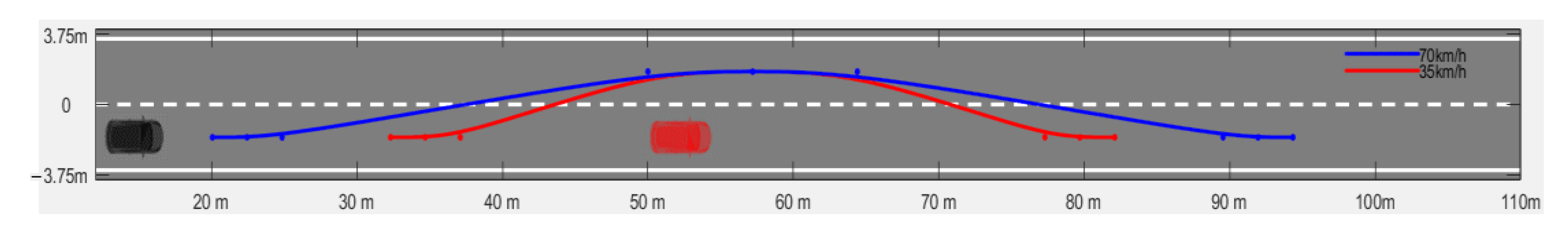
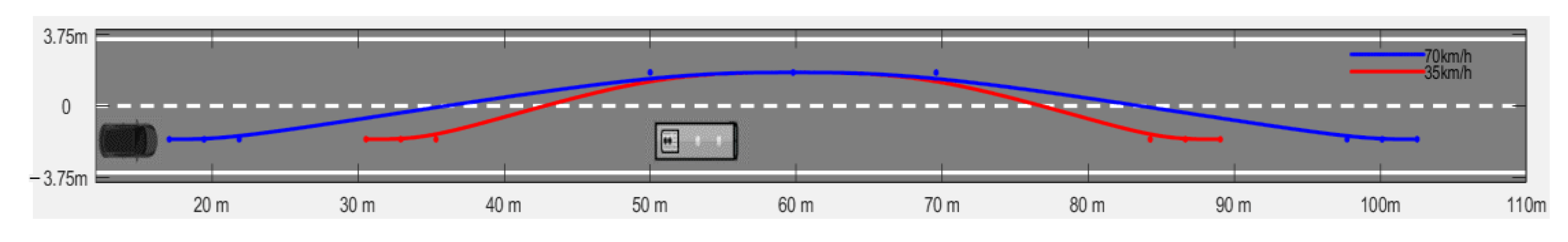
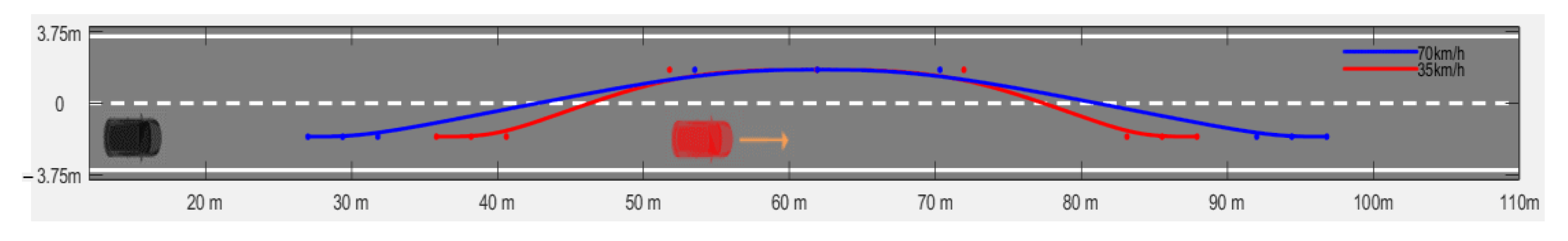
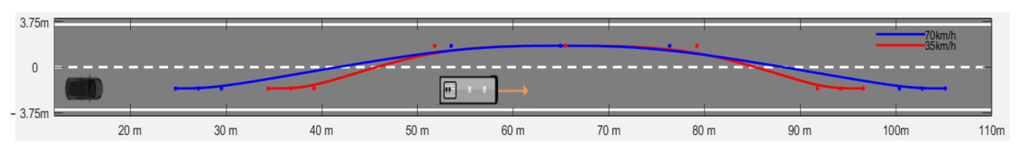
In order to verify the availability of the generated path, a steering control module for autonomous vehicles based on LQR is established in this paper. Then, based on the proposed LQR tracking control algorithm, the MATLAB/CarSim Co-simulation experiments are carried out. For the four obstacle avoidance scenarios in this paper, the scenario of ego-vehicle to avoid dynamic obstacles requires high smoothness of the path. Therefore, a series of co-simulation tests are conducted to verify the availability of the generated paths. In the test scenarios, the speed of the obstacle vehicle is 10 km/h, and the controlled vehicle runs along the planned path at 35 km/h and 70 km/h, respectively. The ego-vehicle detects the obstacle and completes obstacle avoidance, and returns to the original lane after overtaking the obstacle vehicle. The proposed path-planning module generates the obstacle avoidance path according to the obstacle vehicle and environmental information, and the controlled vehicle tracks the generated path based on the proposed LQR algorithm. The simulation parameters of controlled vehicle are shown in

Table 1. Vehicle model parameters.

Model Parameters	Numerical Value/(Unit)
Vehicle mass	1270/(kg)
Vehicle length	4.79/(m)
Vehicle width	2/(m)
Inertia	1536.7/(kg·m2)
Distance from barycenter to front axle	0.907/(m)
Distance from barycenter to rear axle	1.693/(m)
Friction coefficient road surfaces	0.85

.

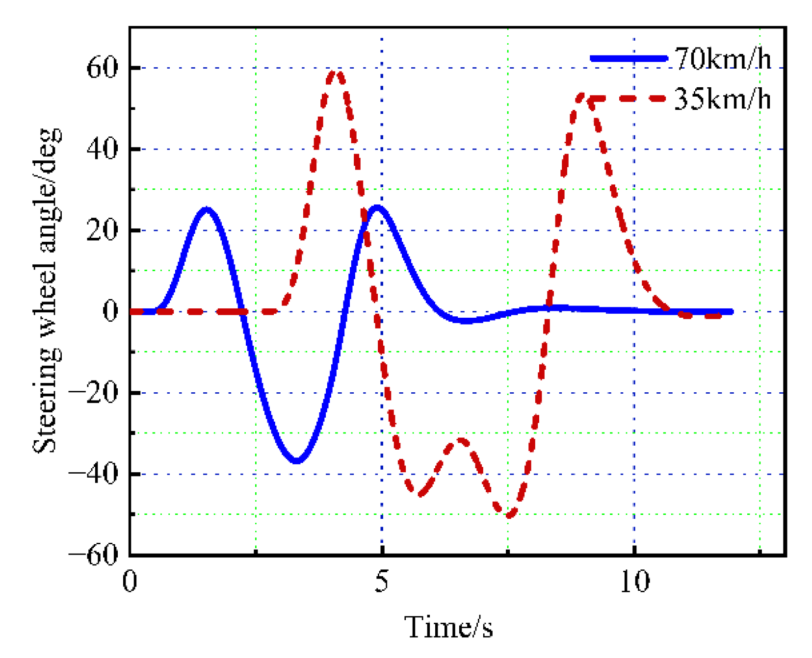
The steering wheel angle curve of the vehicle during the simulation is shown in Figure 9. The steering wheel angle curve is smooth and continuous without oscillation and sudden change. The simulation results show that the generated path is available and conforms to the operating characteristics of human drivers.

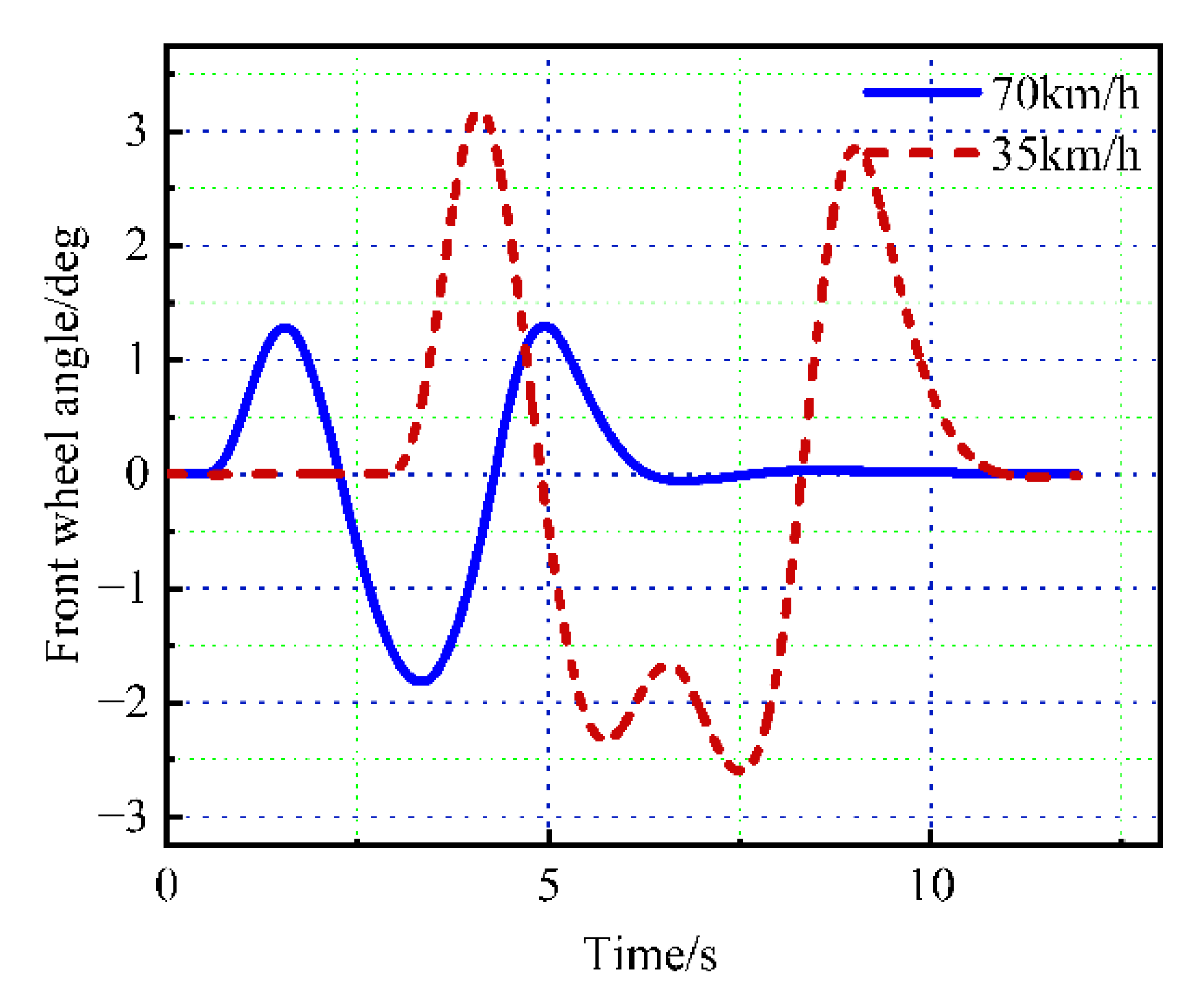
Figure 10 shows the curve of the front wheel angle of the controlled vehicle. As shown in the figure, the front wheel turning angle of the controlled vehicle is between ± 3 deg. The numerical fluctuation range meets the constraint conditions of the front wheel angle, and the front wheel angle curve is smooth, continuous, without oscillation and sudden change.

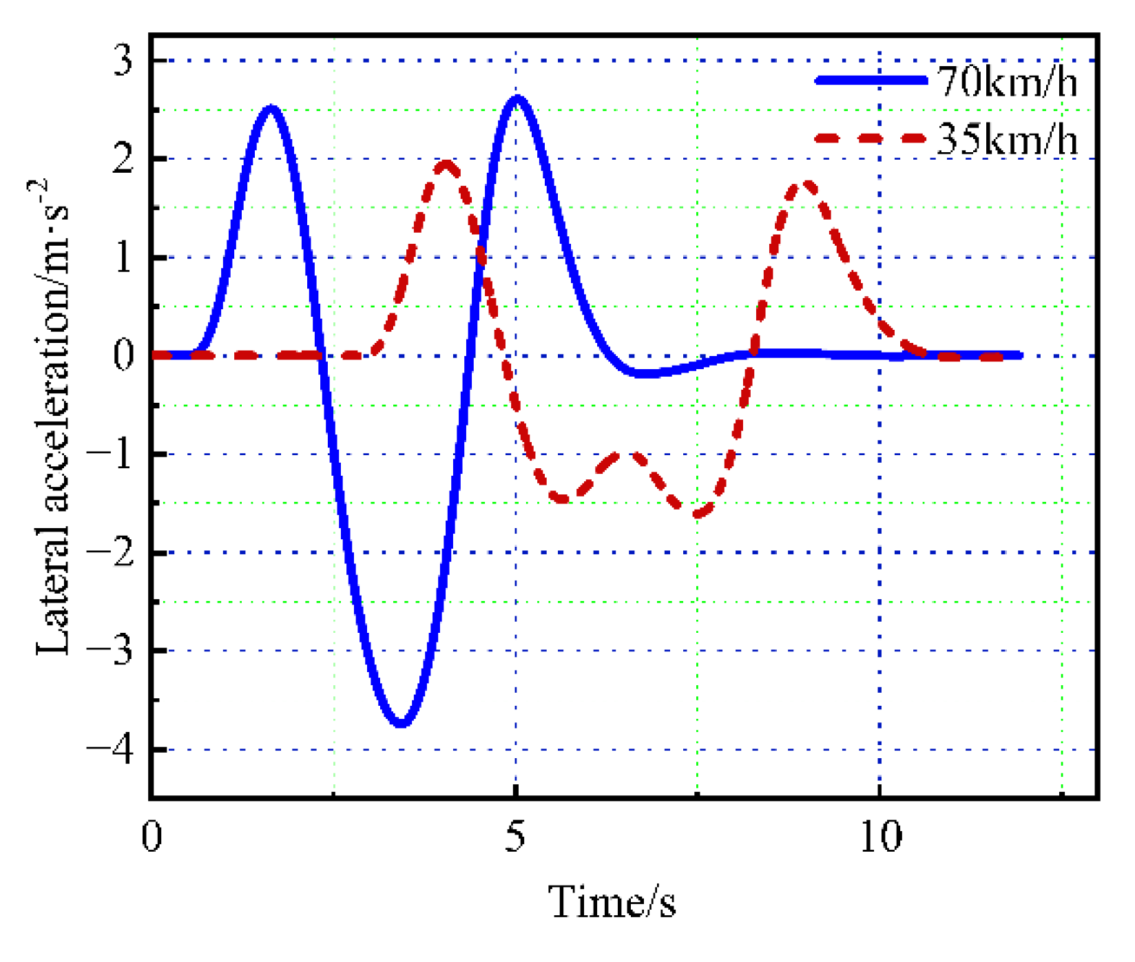
Figure 11 shows the lateral acceleration curve of the controlled vehicle. As shown in the figure, when the controlled vehicle avoids obstacles at a speed of 70 km/h, the lateral acceleration of the vehicle is large, and the maximum acceleration is 3.65 m/s². In this simulation scenario, the vehicle is running on a dry asphalt road. In order to ensure that the vehicle tires are in a linear working area, the maximum lateral acceleration should be less than 3.92 m/s² (0.4 times of the gravitational acceleration). The small lateral acceleration ensures the stability and comfort of the vehicle and proves the availability of the path.

Figure 12a,b, respectively, show the yaw angle and yaw rate curves of the controlled vehicle at different speeds. As shown in the figure, when the vehicle speed is 35 km/h and 70 km/h, respectively, the yaw rate of the vehicle is always maintained within the range of ±11.5 deg/s, and the yaw angle of the vehicle is also maintained within the range of ±11.5 deg. The above results show that the vehicle can track the generated path at different speeds to complete obstacle avoidance operation, and the vehicle is stable throughout the process, without sideslip and tail flick.

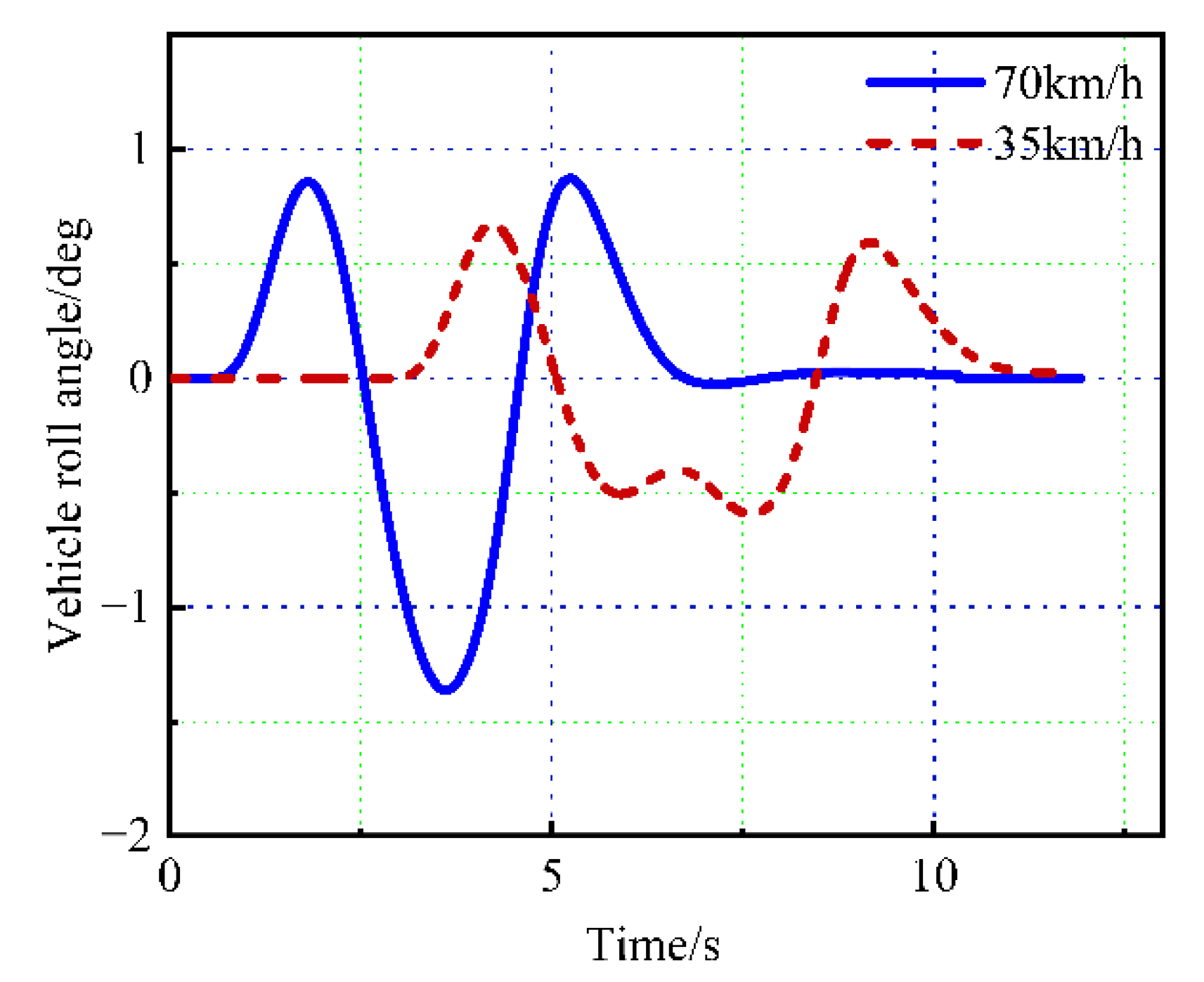
Figure 13 shows the roll angle of the ego-vehicle. The roll angle is an important parameter to indicate whether rollover accident will occur. As shown in the figure, when the controlled vehicle avoids the moving obstacle at 70 km/h, the roll angle value of the controlled vehicle is large. During the simulation, the roll angle range of the controlled vehicle is −1.37 deg to 0.88 deg at the speed 70 km/h. The result shows that the possibility of vehicle rollover accident is low when the controlled vehicle tracks the generated path at high speed.

The simulation results show that the paths generated by the path-planning module are collision free in both scenarios, and the controlled vehicle can accurately track the generated reference path at speeds of 35 km/h and 70 km/h. The key dynamic parameters of the vehicle in the simulation process are analyzed. The results show that the controlled vehicle can ensure the vehicle handling stability when tracking the generated obstacle avoidance paths. The relatively small lateral acceleration can also ensure the driving comfort of the controlled vehicle, and can meet the vehicle dynamics constraints and lane constraints. All results prove that the proposed path-planning algorithm is consistent with the expected lane change results, and it meets the requirements of autonomous vehicle obstacle avoidance path planning.

6. Conclusions

In order to realize the obstacle avoidance function in the dynamic traffic scenario, a path-planning approach based on the B-spline algorithm is proposed in this paper. Firstly, the mechanism of driver path planning is analyzed, and a dynamic risk-identification model based on the support vector machine is proposed. It combines the driver’s risk perception characteristics and a risk model. Then, the B-spline algorithm model is improved based on the risk-identification model. Furthermore, road features, road constraints and dynamic constraints are considered to further optimize the planning algorithm. To verify the path-planning approach proposed in this paper, a co-simulation experiment based on CarSim/Simulink was conducted. Results show that the improved algorithm is effective in static and dynamic obstacles avoidance. The algorithm can generate collision free obstacle avoidance paths, and the paths meet the real-time requirements and dynamic constraints of obstacle avoidance scenario. In addition, the proposed algorithm optimizes the path according to the driver’s operating characteristics, which can further improve the safety and comfort of autonomous vehicles.

Limited by experimental conditions, the proposed path-planning algorithm in this paper is verified through simulation under relatively ideal conditions. The verification scheme of obstacle planning is simplified by using relatively simplified traffic scenarios. In the future, obstacle avoidance path planning in a complex environment with multiple obstacles and variable speed will be studied.