Article

Integration of a Model Predictive Control with a Fast Energy Management Strategy for a Hybrid Powertrain of a Connected and Automated Vehicle

1
Netcom Engineering S.p.a., Via Nuova Poggioreale, 80143 Napoli, Italy
2
Dipartimento di Ingegneria, Università degli Studi della Campania Luigi Vanvitelli, Via Roma 29, 81031 Aversa, Italy
3
Dipartimento di Ingegneria Industriale, Università degli Studi di Napoli Federico II, Via Claudio 21, 80125 Napoli, Italy
*
Author to whom correspondence should be addressed.
World Electr. Veh. J. 2021, 12(3), 159; https://doi.org/10.3390/wevj12030159
Submission received: 15 July 2021 / Revised: 3 September 2021 / Accepted: 15 September 2021 / Published: 21 September 2021

Abstract

:
In the years to come, Connected and Automated Vehicles (CAVs) are expected to substantially improve the road safety and environmental impact of the road transport sector. The information from the sensors installed on the vehicle has to be properly integrated with data shared by the road infrastructure (smart road) to realize vehicle control, which preserves traffic safety and fuel/energy efficiency. In this context, the present work proposes a real-time implementation of a control strategy able to handle simultaneously motion and hybrid powertrain controls. This strategy features a cascade of two modules, which were implemented through the model-based design approach in MATLAB/Simulink. The first module is a Model Predictive Control (MPC) suitable for any Hybrid Electric Vehicle (HEV) architecture, acting as a high-level controller featuring an intermediate layer between the vehicle powertrain and the smart road. The MPC handles both the lateral and longitudinal vehicle dynamics, acting on the wheel torque and steering angle at the wheels. It is based on a simplified, but complete ego-vehicle model, embedding multiple functionalities such as an adaptive cruise control, lane keeping system, and emergency electronic brake. The second module is a low-level Energy Management Strategy (EMS) of the powertrain realized by a novel and computationally light approach, which is based on the alternative vehicle driving by either a thermal engine or electric unit, named the Efficient Thermal Electric Skipping Strategy (ETESS). The MPC provides the ETESS with a torque request handled by the EMS module, aiming at minimizing the fuel consumption. The MPC and ETESS ran on the same Microcontroller Unit (MCU), and the methodology was verified and validated by processor-in-the-loop tests on the ST Microelectronics board NUCLEO-H743ZI2, simulating on a PC-host the smart road environment and a car-following scenario. From these tests, the ETESS resulted in being 15-times faster than than the well-assessed Equivalent Consumption Minimization Strategy (ECMS). Furthermore, the execution time of both the ETESS and MPC was lower than the typical CAN cycle time for the torque request and steering angle (10 ms). Thus, the obtained result can pave the way to the implementation of additional real-time control strategies, including decision-making and motion-planning modules (such as path-planning algorithms and eco-driving strategies).

1. Introduction

Driver and passenger safety has led to a great development of Advanced Driver Assistance Systems (ADASs) in new vehicle projects. ADASs are defined as vehicle-based intelligent safety systems, which could improve road safety in terms of crash avoidance, crash severity mitigation and protection, and post-crash phases. This has become possible thanks to the improvement of sensor technologies installed on the vehicle [1], with the aim to obtain a more comprehensive description of the environment [2]. Moreover, while ADAS allow the vehicle to be automated, communication between vehicles and the road infrastructure is needed to improve driving awareness and prevent the unknown intentions of other road users [3]. Cooperative-Intelligent Transportation Systems (C-ITSs) aim at connecting vehicles to each other and to the road infrastructure, the so-called smart road, increasing traffic safety and efficiency [4]. Therefore, the combination of ADASs and C-ITS results in a Connected and Automated Vehicle (CAV), which opens the way to a new era in the design of cooperative control systems considering both in-vehicle and roadside aspects. In this perspective, the work in [3] described the state-of-the-art and future challenges and opportunities for CAVs, defining the main components of the future transportation systems and considering a holistic approach to deal with challenging tasks such as constrained optimal control problems and energy management strategies.
Concerning control aspects, a CAV requires the adoption of extended nonlinear time-varying models to simulate both the vehicle and the environment, so as to design an efficient control strategy. Moreover, the vehicle to be controlled needs to be subjected to multiple constraints, involving both actuator limits and constraints on maneuvers. Thus, because of its ability to exploit available models and satisfy constraints in control systems, the Model Predictive Control (MPC) is particularly suitable for CAVs. Concerning energy management, the Energy Management Strategy (EMS) of the powertrain deals with the issue of handling the energy flows in the Hybrid Electric Vehicles (HEVs) between the Internal Combustion Engine (ICE), Electric Motor (EM), and battery.
The contribution of this work is twofold and aims at developing an integration strategy that allows running both motion and powertrain control in real-time on a single MCU. First, the MPC strategy proposed in this work controls both the lateral and longitudinal dynamics of a vehicle, considering a simplified single-track model, and it was assumed that not only the motion references for the vehicle and constraints on the speed, but also some of the model parameters that depend on the road conditions, e.g., friction, slope and curvature, would be received from the smart road infrastructure through a C-ITS service. The controller had two outputs, the steering angle of the wheels and the torque request for the powertrain. The torque request was handled by the EMS through the ETESS proposed by the authors in previous works [5,6]. The ETESS aims at minimizing the HEV fuel consumption, and it requires a reduced computational effort with respect to existing strategies (i.e., ECMS) such that it can run on the same control unit of the MPC. This particular implementation was the second main contribution, since for the first time, a vehicle dynamics control algorithm and a powertrain management strategy were demonstrated to run in real time on the same embedded control unit.
The simplified vehicle model and the EMS proposed in this work allowed the embedded real-time implementation of a model-based design module (implemented in the MATLAB/Simulink environment, a typical approach of automotive applications) that connects in cascade the MPC and ETESS. A single Microcontroller Unit (MCU), considering the high-performance Arm-Cortex M7 MCU STM32H743ZI on the development board NUCLEO-H743ZI, was used. The aim of the real-time implementation was to demonstrate by Processor-In-the-Loop (PIL) testing that the computational burden of the cascade between the MPC and ETESS on the same MCU was lower than 10 ms, the typical cycle time of CAN messages for torque and steering, based on the methodology used by the authors in [7].
The execution of both the motion and powertrain control on a single MCU would enable further developments in which the MCU would act as an Internet of Things (IoT) gateway between the vehicle and the surrounding environment. In particular, this gateway would allow the following communications:
  • Vehicle to Vehicle (V2V);
  • Vehicle to Infrastructure (V2I);
  • Infrastructure to Vehicle (I2V).
Thus, the presented solution allows considering a new hardware architecture in which the powertrain and motion controls are directly coupled from a CAV perspective. Furthermore, since a low number of state variables for the vehicle dynamics were used and a simplified EMS was adopted, this study aimed at demonstrating that the approach can be extended with additional control algorithms (i.e., path planning, eco-driving), still using the same MCU and the same CAN cycle time.
The remainder of the paper is organized as follows. Section 2 is a revision of the state of the art about MPC for CAVs and about EMS. Section 3 describes the proposed method to: (i) design a simplified but complete nonlinear single-track ego-vehicle model and its linearization in order to allow the implementation of an adaptive MPC; (ii) define the powertrain model and the ETESS strategy. Section 4 describes: (i) the comparative assessment between ETESS and ECMS; (ii) the PIL test on the selected MCU. Section 5 and Section 6 discuss the results as well as the limitations of the current approach and future developments, respectively.

2. Related Work

This section presents the relevant scientific background about MPC for CAVs and EMS for hybrid powertrains.

2.1. MPC for CAVs

Recent technologies and control strategies have found several fields of application for tracking problems. For example, in [8], a novel control strategy has been proposed for enhanced operation and control of DC microgrid systems (based on photovoltaic modules, battery storage systems, and DC load), enabling a maximum power point tracking (MPPT). In [9], the authors propose an adaptive neuro-fuzzy inference system (ANFIS) for blade pitch control of the wind energy conversion systems (WECS) instead of the conventional controllers. Additionally, MPC has acquired more and more robustness and has been applied in various fields. For example, the work of [10] shows the robustness of MPC application for robotic manipulators, in order to track regular and irregular trajectories, comparing it with other techniques. The work in [11] shows the robustness of MPC for data-driven models. In the field of CAVs, MPC has been indicated as the most promising control technique, as reported in [3], due to: (i) its ability to handle Multi-Input-Multi-Outputs (MIMO) systems (without the need to design more PIDs and corresponding decouplers); (ii) proven and fast optimization methods; (iii) its ability to handle constraints on control variables (and their relative rate of charge) and outputs variables. Thus, in this paper, the choice of control strategy, given the application context, fell on MPC.
MPC is not new in autonomous driving applications, both for longitudinal vehicle dynamics and lateral control. In [12], an MPC acts as an upper controller for platooning to obtain the desired longitudinal acceleration and a PID acts as lower controller to determine either engine throttle or brake input. In [13], a step-by-step linearized MPC has been used for longitudinal dynamics starting from a low-order model. In [14], an adaptive MPC is proposed for lateral control in lane keeping problems, where longitudinal velocity is assumed constant and the goal is to minimize the distance from lane center line and the steady state heading angle error, while satisfying the respective safety constraints. In [15], the integration of a Linear-time-varying Model-predictive-control (LTV-MPC) is presented. The model is designed to stabilize a vehicle during sudden lane change or excessive entry speed in curve, with a slip controller that converts the desired longitudinal tire force variation to pressure variation in the brake system. The approach uses a 3DOF vehicle model taking into account both yaw rate and side slip angle of the vehicle, while the slip controller is a gain scheduled proportional controller with feed-forward action, validating the performances through simulation.
The MPC strategy proposed in this work acts as a high-level controller, operating as an interface between the Smart Road and a hybrid powertrain. Thus, on one side the MPC manages vehicle maneuvers acting on the steering angle and wheel torque, based on the information from the surrounding environment, considering:
  • Intelligent Speed Adaptation (ISA) from Smart Road Infrastructure (e.g., point-to-point speed);
  • ADAS Maps (e.g., TomTom) and systems to determine steering maneuvers;
  • Environmental and road data (e.g., wind speed and road friction) provided by Infrastructure to Vehicle (I2V) communication;
  • Parameters and measurements from vehicles located ahead (e.g., its acceleration, speed and mass) provided by Vehicle to Vehicle (V2V) communication;
  • ADAS functionalities to maintain a certain safety distance from the vehicle located ahead.
On the other hand, the torque request provided by MPC is handled by the EMS through the ETESS strategy proposed by the authors in previous works [5,6]. In this way, the MPC occupies two layers of the real-time control for CAVs presented in [3]: (i) motion control; (ii) powertrain control.
MPC implementation on automotive Electronic Control Units (ECUs) is difficult due to real-time constraints. In fact, in the automotive field, the trend predicts the usage of Field Programmable Gate Arrays (FPGAs) [16] and there are feasibility studies in the field of vehicle platoons [17], but not yet real applications on homologated CAVs.
For this reason, the MPC presented in this work has been tested on a real MCU, not based on FPGA but on a high-performance Arm-Cortex M7 MCU. This kind of MCUs will probably drive the future of the mobility [18,19], due to their low costs and good performance. In this work, the development board NUCLEO-H743ZI equipped with a STM32H743ZI MCU [20] has been used, due to the possibility provided by ST Microelectronics to enable PIL Testing [21] in the MATLAB/Simulink environment, which is the main software development tool for Model-Based-Design in the automotive field. PIL testing is a fast procedure that does not require high investments (i.e., buying a real-time Hardware In the Loop simulator) and setup times. Thus, it is particularly suitable for a real-time test at an early stage of a project [7].

2.2. EMS for Hybrid Powertrains

Additionally, EMS for hybrid powertrains has been widely investigated in the current literature. The task of EMS is to solve a minimization problem, subjected to system dynamics and constraints, defining a constrained optimization problem. As an example, refs. [22,23] report that the limited energy storage capability of the batteries, for an optimal control formulation, may be interpreted as a terminal state constraint. Hence, since the HEV battery cannot be recharged through the grid, its terminal charge is fixed as a constraint, usually equal to its initial/nominal value. If the driving future information is known, the problem can be simply solved by employing Global Optimization Strategies such as the Pontryagin Minimum Principle (PMP) [24] or Dynamic Programming (DP) [25]. However, knowing the entire driving cycle means it is impossible to implement it for use in a real vehicle due to the lack of future information. These strategies are usually defined as offline since they are used as “theoretical targets” to find the optimal results obtained by the hybrid vehicle. On the other hand, the Local Optimization Strategies (LOSs) are based on present or past information, and are the so-called online strategies. In this case, the problem is subdivided into a sequence of local problems. Hence, there is no need for information about the entire driving mission, making possible its application to a real vehicle. It is worth underlining that the LOS does not provide the optimal solution to the control problem, but only a suboptimal one. The most known is the Equivalent Consumption Minimization Strategy (ECMS) [26], which can be considered as an online variant of the PMP. Recent works introduced in the optimization problem the possibility to adapt the EMS according to forecasts of vehicle velocity or power request at the wheels, such as in [27,28].
In this work, the EMS uses the ETESS strategy, proposed by the authors in [5,6]. ETESS aims at minimizing HEV fuel consumption, and it requires a reduced computational effort with respect to existing strategies (i.e., ECMS), such that it is more suitable to the be run on the same control unit of the MPC.

2.3. Integration of MPC with EMS

The integration of MPC with EMS is examined in [29] as an evolution of energy management and a future trend, also discussing the need of validation processes based on Model In the Loop (MIL), Software In the Loop (SIL) and Hardware In the Loop (HIL). In [30], a survey about the state of the art in EMS for connected HEVs and PHEVs (Plug-in HEVs) has been presented, considering, in particular, MPC for eco-driving on connected vehicles using V2I communication. In [31], an MPC for HEVs in car-following scenarios has been implemented to investigate the interplay between fuel economy, vehicle exhaust emissions, and inter-vehicle safety. Specifically, an MPC-based controller is developed to optimize the vehicle speed and engine torque for better fuel economy and fewer exhaust emissions while ensuring inter-vehicle safety. In [32], an MPC-based energy management strategy is proposed, in which the predicted velocity and SoC (State of Charge) trajectory is regarded as reference signal, demonstrating that the fuel economy of HEV is improved by considering velocity prediction and SoC trajectory planning.
In this work, an embedded real-time implementation of a model-based design module that connects in cascade MPC and ETESS is proposed, and a low-cost test strategy, named PIL, has been used in order to verify, at this first step of the project, the real-time execution of the coupled motion and powertrain controls.

3. Methodology

This section first shows a complete nonlinear ego-vehicle model, which is then linearized to allow the design and implementation of an adaptive MPC control strategy. This strategy implements functionalities for autonomous driving, considering as control variables the steering angle at the wheels and wheels’ torque. The last control variable provides the power demand for the implemented EMS.The second part of this section reports the powertrain and driveline model and, finally, the ETESS implementation.

3.1. Vehicle Model

In order to design the MPC, a simplified but complete ego-vehicle nonlinear single-track model for combined longitudinal and lateral vehicle dynamics is used. Then, two errors (for lateral offset and yaw angle) are modeled to enable the development of Lane Keeping Systems (LKS). Eventually, a simple car-following model is derived to consider the relative distance and velocity from an ahead vehicle. All quantities are expressed in SI units unless otherwise explicitly stated.
This model will allow designing Adaptive Cruise Control (ACC), Lane Keeping System (LKS), and Emergency Electronic Brake (EEB) for ADAS, but it can be used for cooperative driving control strategies as well, considering the V2X (Vehicle to everything) and I2V (Infrastructure to Vehicle) communications between vehicle and Smart Road, for example, by using the C-ITS services ISA (Intelligent Speed Adaptation) or in-Vehicle SPeeD limits (VSPD) [4].

3.1.1. Single-Track Model

The single-track model is derived from the four-wheeled model presented in [33], according to the following three assumptions
1.
Only the front wheels are considered to be driving, so the overall wheels torque τ w is the sum of the torque at front wheels during accelerations. Furthermore, τ w is assumed as the sum of the torque at all the wheels during braking;
2.
The steering angles of the front wheels are equal to δ and the small angle approximation is used [34], considering that the control range on the steering angle at the wheels is [−5, 5]°; thus, sin δ δ and cos δ 1 ;
3.
The longitudinal slip ratio σ i j (the subscripts i j indicate the positioning of the wheel on the vehicle, i.e., front right f r , front left f l , rear left r l and rear right r r ) is considered negligible and defined as follows
σ i j = R e f f ω i j v x v x , during acceleration R e f f ω i j v x R e f f ω i j , during braking
where R e f f is the effective wheel radius, ω i j is the specific wheel speed and v x is the longitudinal vehicle speed [34].
From assumption 3, it follows that
R e f f ω i j = v x ,
From the wheel dynamics, defined in (3), the longitudinal tire forces F x i j can be derived, depending on the longitudinal acceleration, considering (2), and on wheel torque for each wheel τ w i j
I ω ω ˙ i j + R e f f F x i j = τ w i j ,
where I w is the moment of inertia of the wheel [33]. With the assumptions above and considering the lateral speed v y and the yaw angle rate ω ψ , a simplified nonlinear single-track model is obtained, characterized by three state variables x d y n = [ v x v y ω ψ ] T in three equations
m + 4 I w R e f f 2 v ˙ x = τ w R e f f + m ω ψ v y L 3 ω ψ 2 F a e r o F r e s t o t m g s i n θ + 2 δ C α δ v y + L f ω ψ v x ,
m v ˙ y = m ω ψ v x + L 3 ω ˙ ψ + δ τ w R e f f 2 I w v ˙ x R e f f 2 + 2 C α δ v y + L f ω ψ v x + 2 C α v y L r ω ψ v x ,
I 3 ω ˙ ψ = L 3 v ˙ y + L 3 ω ψ v x + 2 L f δ τ w 2 R e f f I w v ˙ x R e f f 2 + 2 L f C α δ v y + L f ω ψ v x + + 2 L r C α v y L r ω ψ v x ,
where m is the vehicle mass, the term F a e r o is the aerodynamic drag force, defined as F a e r o = 0.5 ρ A C d ( v x + v w ) 2 , with ρ being the air density (possibly provided by the Smart Road via I2V based on the altitude; in this case, it is assumed at sea level), A is the maximum vehicle cross area, C d is the drag coefficient depending on vehicle body shape and v w is the wind speed (provided by the Smart Road via I2V). The term F r e s t o t refers to the sum of the front and rear wheels’ rolling resistance forces, defined as F r e s t o t = C r ( F z f + F z r ) = C r m g cos θ , where C r = 0.01 ( 1 + v x / 100 ) is the rolling resistance, F z f and F z r are the normal tire forces, at the front and at the rear of the vehicle, calculated as in [34] and their sum is m g c o s θ , where θ is the road slope angle (supposed to be known by Inertial Measurement Unit in vehicle and/or ADAS Maps and/or I2V). The term m g s i n θ is the gravity force component along the vehicle longitudinal axis, while C α is the cornering stiffness of the tire, L f , and L r are the distances of the front and rear tire centers from the vehicle Center of Gravity (CoG), respectively. The terms L 3 and I 3 are defined in [33] depending on the wheel masses, the vertical moment of inertia, and the front-axle track of the vehicle.

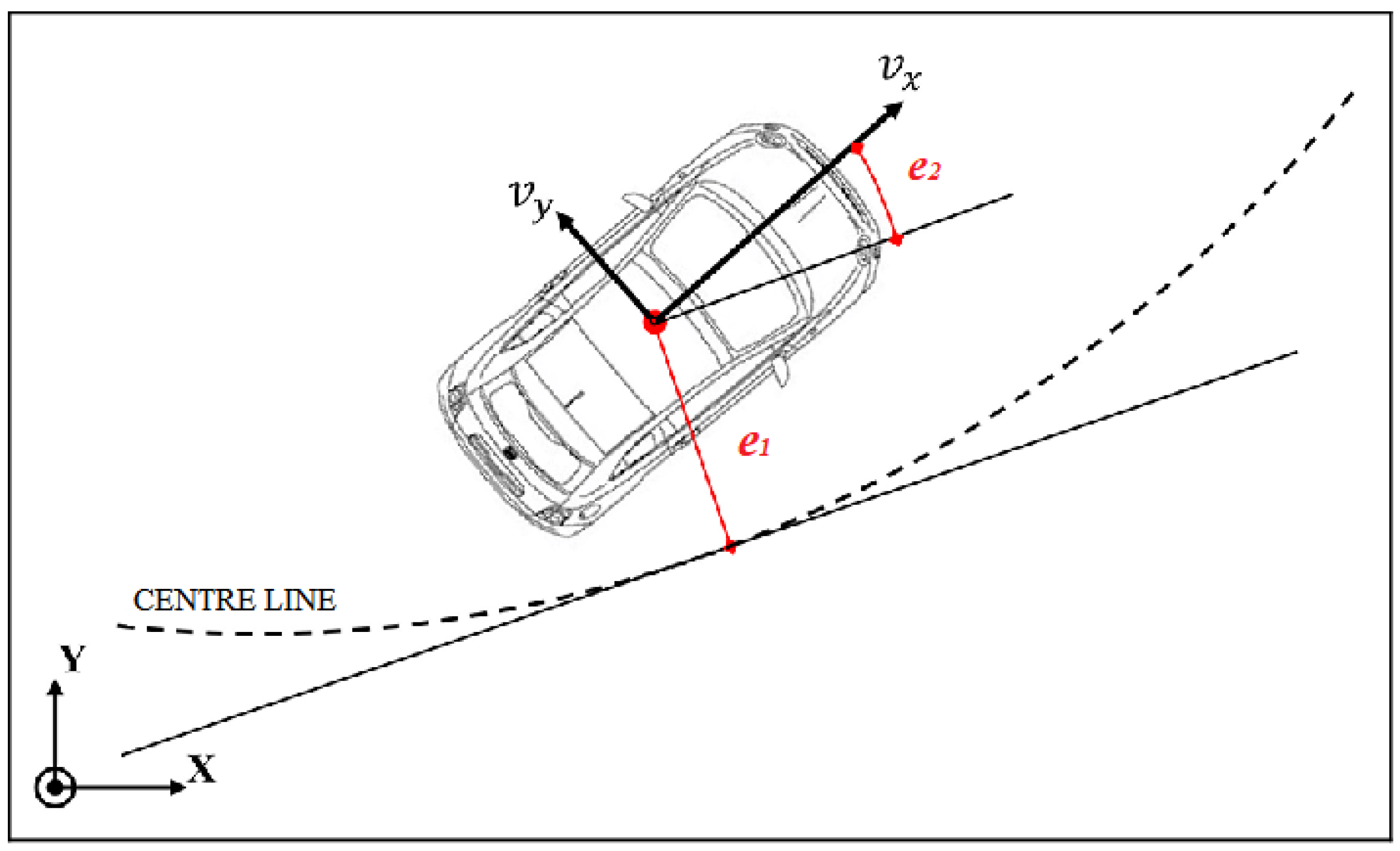
3.1.2. Equations of Errors with Respect to the Road

In order to implement an LKS, a dynamic model is considered. It is based on two additional state variables, expressed in terms of position and orientation errors with respect to the road reference system [34]. Thus, as shown in Figure 1, defining e 1 as the lateral displacement (the distance of the CoG of the vehicle from the center line of the lane) and e 2 as the relative yaw angle error concerning the road centerline (angle between the longitudinal velocity direction and the tangent to the center line), considering the road radius R r is large so that the small angle assumptions can be made and supposing that the road curvature R c = 1 / R r is known from in-vehicle ADAS map and/or I2V communication, the desired yaw rate of the vehicle is defined as in [34] as
Ψ ˙ r e f = R c v x .
The dynamics of lateral displacement, according to [34] is
e ˙ 1 = v y + v x e ψ ,
being e ψ = Ψ Ψ r e f , where Ψ is the yaw angle of the vehicle ( Ψ ˙ = ω ψ ), this implies that
e ˙ 2 = ω ψ R c v x .
Defining x e = [ e 1 e 2 ] T , two additional states are added to the ego-vehicle model, which are assumed as measurable by ADAS sensors and maps.

3.1.3. Car-Following Model

If the ego-vehicle is preceded by another car, the relative distance and velocity from the ahead vehicle have to be considered. These measures are available considering radar and/or LiDAR and/or camera sensors commonly used in ADAS.
This study considers both the presence of an ahead vehicle and V2V (Vehicle to Vehicle) communication; thus, two additional states are necessary, e.g., the velocity of the vehicle located ahead v a h and the relative distance d r of the ego-vehicle from the latter, as shown in Figure 2. Assuming the availability of a Smart Road, this model takes into account the road slope θ , the wind speed v w , and the road friction σ r provided by C-ITS (e.g., I2V) services. In addition, since the MPC acts on the ego-vehicle only, the traction/braking force of the ahead vehicle u a h is assumed to be known thanks to the V2V communication, considering the longitudinal slip ratio to be negligible. Thus, the additional states to consider for the complete ego-vehicle model are defined below
m a h v ˙ a h = u a h σ r v a h K a h ( v a h + v w ) 2 m a h g sin θ ,
d r ˙ = v a h v x ,
where K a h = 0.5 ρ A a h C d a h ( A a h is the maximum cross-area of the ahead vehicle and C d a h its drag coefficient) and m a h is the ahead vehicle mass [34]. All these parameters are assumed to be known and transmitted through V2V to the ego-vehicle. Then, the states x e x t = [ v a h d r ] T are added to the other state variables to define the complete ego-vehicle model, as detailed in the next section.

3.1.4. Complete Nonlinear Ego-Vehicle Model

The complete model of ego-vehicle is featured by the following states, control inputs and outputs
x v = [ x d y n x e x e x t ] T , u v = [ τ w δ ] T , y v = [ v x e y e ψ d r ] T
and the corresponding state space equations are (4a)–(4c), (6), (7), (8a), (8b).

3.1.5. Linearization of the Complete Ego-Vehicle Model

Aiming to allow MPC to work around a reference trajectory, the nonlinear model (9) is linearized if the reference speed and/or road curvature change, even at each iteration if needed, in order to obtain a linear time-varying system [35]. The reference speed v r e f is assumed to be known via C-ITS and sensor fusion of radar and/or LiDAR and/or the camera provided by ADAS. For the same reason, road curvature and therefore Ψ r e f are known as well. The wheel steering reference δ r e f is given by the following relation [34]
δ r e f = 1 R c ( L v + m v r e f 2 C α r L r C α f L f 2 C α f C α r L v ) ,
where L v = L r + L f , C α r = C α f = C α , considering single-track model assumptions. The torque set point τ a during acceleration is given by (4a) at the equilibrium, while during braking, the brake model [36] is adopted to get the set-point trajectory, e.g.,
P ˙ = 150 K c u b τ b s P τ b s ,
where P is the amount of pressure produced behind the brake disk, while applying the brake pedal and K b P is the brake torque, with K b being the gain of the braking system. The parameter τ b s is the lumped lag obtained by combining two lags relating to the dynamics of the servo valve and the hydraulic system, K c is the pressure gain and u b is the percentage of pressure on the brake pedal. Moreover, u b is provided by a simple driver model featured by a PI control acting on the derivative of the speed reference, to model a driver’s behavior during braking, which is useful to obtain a reference.
The set-point trajectory for lateral velocity v l a t is given by the solution v y of (4b) at the equilibrium, while the set points for e 1 and e 2 are both equal to zero. Eventually, the set point of v a h is assumed to be known via ADAS and V2V and the desired relative distance is defined as
d d e s = d s a f e = L + T h v x ,
where d s a f e is the theoretical safety distance depending on the ego-vehicle length L and a response time T h [ 1.5 , 2 ] s of the ego car during braking [7].
The state, input and output variables of the linearized system are defined as
δ x v = [ x d y n x ¯ d y n x e x ¯ e x e x t x ¯ e x t ] T ,
δ u v = [ τ w τ ¯ s δ δ ¯ s ] T ,
δ y v = [ v x v r e f e 1 e ¯ 1 e 2 e ¯ 2 d r d s a f e ] T ,
where x ¯ d y n = [ v r e f v l a t Ψ ˙ r e f ] T , x ¯ e = [ e ¯ 1 e ¯ 2 ] T = [ 0 0 ] T and x ¯ e x t = [ v r e f d s a f e ] T are the set points for the states of the complete model; τ ¯ s = K b P during braking, while τ ¯ s = τ a otherwise is the set point for the wheel torque; δ ¯ s = δ r e f is the one for the wheel steering angle; v r e f is the reference speed.
Thus, the linearized time-varying system, obtained from Jacobian computation, in the continuous time is
δ x ˙ v ( t ) = A c ( t ) δ x v ( t ) + B c ( t ) δ u v ( t ) ,
δ y v ( t ) = C c δ x v ( t ) ,
where A c ( t ) and B c ( t ) are the dynamic matrix and the input matrix (time varying from linearization process), respectively, and C c is the output matrix (constant, because it selects only the four states featuring the outputs) [37]. For MPC purposes, this model is discretized as
δ x v ( k + 1 ) = A m ( k ) δ x v ( k ) + B m ( k ) δ u v ( k ) ,
δ y v ( k ) = C m δ x v ( k ) ,
where A m ( k ) = A c ( k ) + I n 1 Δ t , B m = B c ( k ) Δ t and C m = C c are the dynamic, input and output matrices of the discretized model [37], Δ t is the sampling time and I n 1 is the identity matrix of dimension n 1 (number of states of the complete ego-vehicle model).
The sampling time is chosen equal to 10 ms (the typical cycle time of the CAN message for the torque request). The list of parameters and their values used in the ego-vehicle model is shown in Table 1. Those values refer to a commercial small utility vehicle.

3.2. Model Predictive Control

MPC aims to optimize a quadratic cost function by realizing two goals: minimizing the error between the outputs of the plant model (provided by linearization of the complete ego-vehicle model) and the references and enforcing the constraints. This control strategy is able to obtain prior knowledge of the linearized model by predicting its future behavior.
The preliminary steps considered in the design of the controller via the MPC method are:
1.
Modeling the system to control, described by Equations (4a)–(4c), (6), (7), (8a), (8b), whose states, inputs and outputs are defined in Equation (9).
2.
Linearizing and discretizing the model, as described in Equations (13a)–(13c) and (14a)–(15b).
3.
Augmenting the model, by concatenating states and outputs of the linearized and discretized model [38].
4.
Defining a cost function.
5.
Setting the constraints on input and/or output variables.
Then, an optimization algorithm finds the optimal solutions for the unconstrained case and for the constrained case valid for the considered model. In this way, an adaptive MPC on the time-varying linearized and discretized system is obtained.
The control system predicts the q outputs ( q = 4 in this work) over an established time window. In particular, it predicts N p values ( N p = 10 in this work) of the outputs, where N p is called “prediction horizon”. Thus, MPC computes, at each iteration, a control trajectory (for each control variable) of N c samples, where N c ( N c = 5 in this work) is called “control horizon”. However, according to the Receding Horizon Control (RHC) approach, only the current p inputs ( p = 2 in this work) are provided to the plant under control, i.e., the wheel torque and steering angle of the vehicle.
In order to obtain a sub-optimal solution, the procedure described in [38] is used, based on Hildreth’s method, particularly useful for fast MPC implementation, as showed in [39,40,41], both for automotive and other kind of applications (i.e., UAV and underwater vehicles).
In this work, the linearized and discretized model is augmented considering it as increment of the control signal Δ u = δ u v . Then, a quadratic cost function is considered, defined as:
J = ( Y r e f Y ) T ( Y r e f Y ) + Δ U T Q Δ U
where Y r e f R N p q is the vector of the current q references replicated N p times, Y R N p q is the vector of the evaluated N p output predictions, obtained through algebraic passages and Δ U R N c p is the vector of control inputs over the control horizon [38]. Furthermore, Q R ( N c p ) × ( N c p ) is a diagonal matrix with suitable weights for each value of the control trajectory Δ U . In detail, Q = blockdiag ( Q p , , Q p ) , with Q p = diag ( q t b , q δ ) , where q t b ( q t b = 50 in this work) refers to traction and braking wheel torque and q δ ( q δ = 7 e 4 in this work) refers to steering at the wheels. The weights are here chosen based on the simulation results obtained by Model In the Loop (MIL) tests in MATLAB/Simulink (version R2020b) for the test cases discussed in the last section.
Within the MPC control framework, in addition to minimizing the index in (16), inequality constraints for current inputs, future inputs and future outputs can be set according to [38]. To reduce the computational load and given the RHC control logic, inequality constraints are set only for the current inputs and on the relative distance from the ahead vehicle, as:
τ m i n τ ¯ s δ m i n δ ¯ s δ u v ( k ) τ m a x τ ¯ s δ m a x δ ¯ s ,
d ¯ s v d r ( k ) d s a f e ( k ) 100 .
In particular, in (18), a soft constraint on d r is imposed, to accept at most a term equal to d ¯ s v ( 1 m in the case studies) below the theoretical safety distance d s a f e . Furthermore, the upper bound of 100 m is selected to keep the distance between the two vehicles limited.
The constrained problem can be solved only locally and, in order to obtain a fast computational burden with the objective to run adaptive MPC in a CAN cycle time ( 10 ms), as will be shown in the results section, in this work Hildreth’s Quadratic Programming procedure is used. Then, defining Δ U R H C as the first two elements of the obtained sub-optimal control, by adding to Δ U R H C the set points of control variables, the corresponding vector of control inputs u v is obtained.
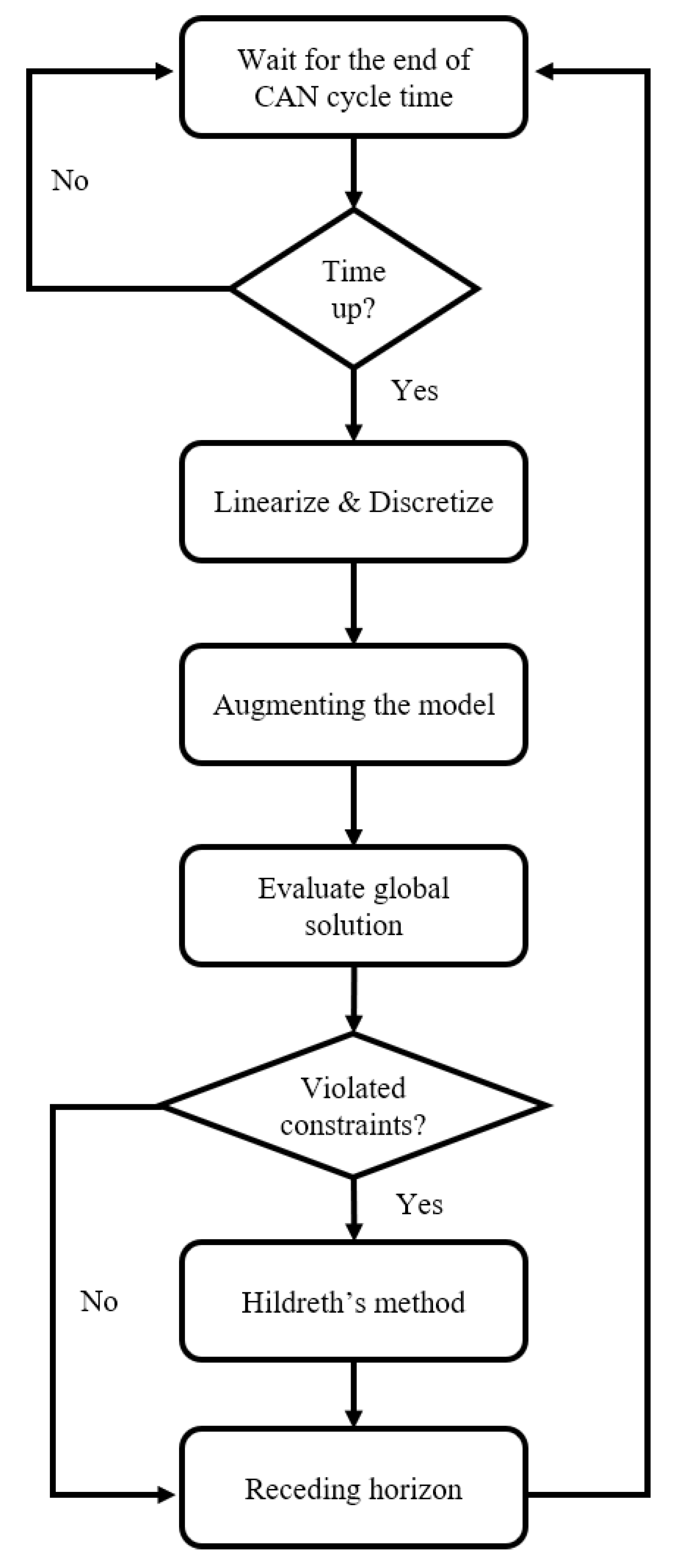
The overall flow chart for MPC implementation through model-based design approach and for MPC execution on a real MCU is shown in Figure 3. Thus, at each time step the control algorithm waits for a new CAN message containing updated vehicle and environmental data (i.e., reference speed from C-ITS and/or ADAS sensors, road curvature, vehicle speed, lateral displacement, yaw angle error and relative distance). Then, when new data are available, the algorithm at first executes linearization and discretization, then the linearized model is augmented and MPC evaluates the global solution. If constraints are not violated, then the receding horizon allows to update the wheels torque and the steering angle at the wheels at the current time step, and then the execution returns to wait for a new CAN message. If there is a violation on constraints, then Hildreth’s method is executed in order to find a sub-optimal solution. Thus, the receding horizon is applied. Eventually, the execution restart waiting for a new CAN message.

3.3. Powertrain and Driveline Model

The vehicle investigated in this work presents a combined series-parallel powertrain composed of an ICE, two electric motor/generator units ( E M and E G ), a battery pack ( B a ), a power converter ( P C ), three clutches ( C l 1 , C l 2 , and C l 3 ), a differential ( D i f f . ) and three gear-boxes ( G B 1 , G B 2 , and G B 3 ). The powertrain schematic is depicted in Figure 4. Either series or parallel driving can be activated, depending on the clutches position. Battery charging can be realized though E G engaging C l 3 . Possible driving modes and the corresponding engagement/disengagement of the clutches are summarized in Table 2. The presence of three clutches, on one side, complicates powertrain control, but, on the other side, avoids loadless operation when a unit is not used, reducing friction losses.
A static model of the powertrain and the driveline was implemented in the Simulink environment. It includes all components depicted in Figure 4, where I C E , E M , and E G are described by their efficiency maps, while P C and B a are characterized by fixed parameters, listed in Table 3.

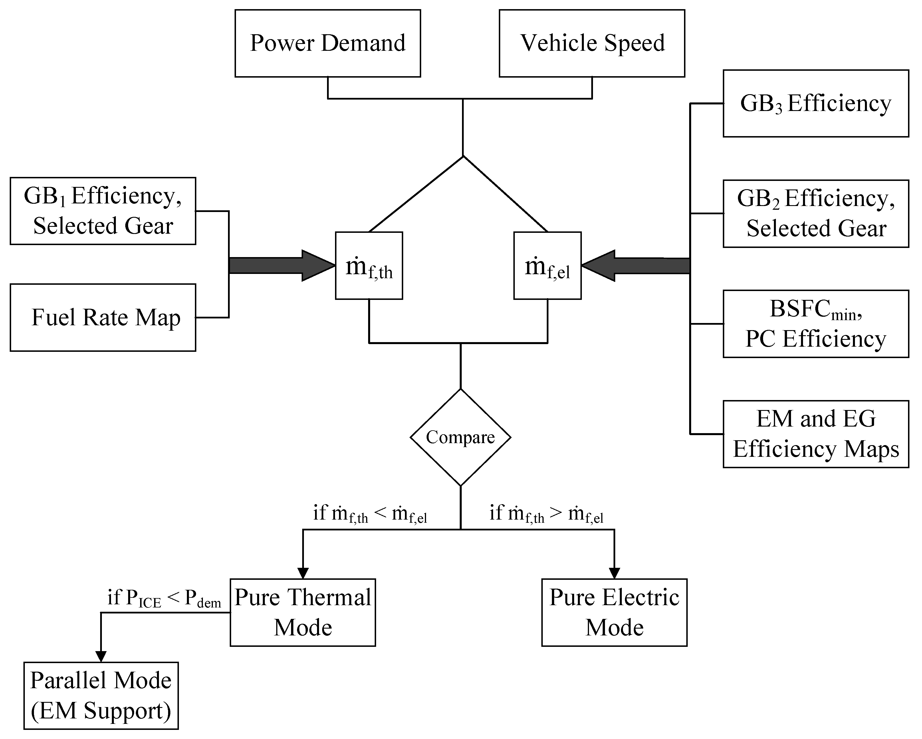
3.4. Efficient Thermal Electric Skipping Strategy

The ETESS is a simplified logic that replaces the conventional power split approaches with an alternative utilization of the thermal and electric units for the fulfillment of the power demand at the vehicle wheels ( P d e m ). The power demand is evaluated starting from the wheels torque provided by MPC as follows:
P d e m = v x τ w R e f f
The choice between these two motors depends, at each time, on the comparison between the actual fuel rate of the I C E (when it operates to fully satisfy the power demand, if possible) and an equivalent fuel rate associated with the pure electric driving of the vehicle (Figure 5).
The identification of the equivalent fuel rate ( m ˙ f , e l ) is based on the concept that, in a series configuration, the power delivered by the E M to fulfill the power demand at the wheels was produced by the thermal engine in an undefined time, while working in its operating point of minimum brake specific fuel consumption ( B S F C m i n ). Since such power flux from the thermal engine to the wheels involves some losses in the G B 3 , in the E G , in the P C , in the E M , in the G B 2 , and in the differential, the equivalent fuel rate in the pure electric mode is defined as follows:
m ˙ f , e l = c 0 · P d e m · B S F C m i n η G B 3 · η E G · η P C 2 · η E M · η G B 2 · η D i f f ,
where c 0 is a tuning constant introduced to realize the energy balance for the battery between the beginning and the end of the driving cycle, η E G is the efficiency of the E G , η E M is the efficiency of the E M , η P C is the efficiency of the power converter, η G B 3 is the G B 3 efficiency, η G B 2 is the G B 2 efficiency and η D i f f is the efficiency of the differential. The Joule losses occurring into the battery pack are not explicitly considered in this formulation to preserve its mathematical simplicity.
The fuel rate in the pure thermal mode ( m ˙ f , t h ) only depends on the power demand, on the GB1 efficiency ( η G B 1 ) and on the losses in the differential:
m ˙ f , t h = P d e m · B S F C η G B 1 · η D i f f .
The B S F C is the actual brake specific fuel consumption of the ICE operating with the load and the speed related to the power demand at the wheels and the vehicle velocity, respectively.
The only degree of freedom for the evaluations of both m ˙ f , t h and m ˙ f , e l is the gear selection of the related gear-boxes. The latter is straightforwardly carried out by choosing the one that leads to the lowest fuel rate, complying with the constraints on minimum/maximum rotational speed and on maximum deliverable torque. Given the above definitions, the strategy for the selection between the pure electric mode and the thermal engine driving can be summarized by the following two inequalities
m ˙ f , t h m ˙ f , e l , pure thermal mode m ˙ f , t h > m ˙ f , e l , pure electric mode .
In summary, the ETESS method can be considered as a specialization of the ECMS, in which the only allowed power split values are either 0 or 1.
The introduction of such simplification is expected to involve a certain penalization of the fuel economy compared to the P M P or the ECMS, but, on the other hand, a much reduced computational effort. In the ETESS approach, in fact, the choice between the pure thermal mode and the pure electric driving does not need any discrete map exploration: the I C E operating point to be inquired for the evaluation of m ˙ f , t h is univocally determined by the tractive power demand, the vehicle speed, and the losses along the driveline from the wheels to the engine (such evaluation has to be repeated only for the available gears of the gearbox linked to the ICE). Similarly, m ˙ f , e l is univocally determined by the traction power demand, the vehicle speed, the losses along the driveline, and the dissipation in the electric units.
To avoid the onset of chattering, the actual switch between pure thermal driving to pure electric one (and the contrary) is realized only when the fuel rate advantage deriving from the driving mode switch exceeds the one in the current mode of a tunable quantity (about 0.22 kg/h in the present work).
The ETESS logic activates the parallel mode only when the I C E is not able to fully supply the vehicle power demand by itself. In this case, the I C E works at the maximum rated power, while the E M furnishes the remaining power to fulfill the power demand. The regenerative braking (which is activated when the wheel power demand becomes negative) is realized by the E M .
Since the aforementioned definition of the equivalent fuel rate needs an a priori knowledge of the vehicle speed to correctly select the c 0 tuning constant, the ETESS, in the above-presented formulation, can be considered an offline strategy. For this reason, to realize a real-time implementation, Equation (20) can be replaced by the following one:
m ˙ f , e l = c ¯ 0 s c o r r P d e m B S F C m i n η G B 3 η E G η P C 2 η E M η G B 2 η D i f f ,
where c ¯ 0 is a vehicle-dependent constant (which is obtained by preliminary simulations performed in offline mode, where c ¯ 0 is adjusted to realize a battery charge sustaining driving mode) and s c o r r is an adaptive correction depending on the current SoC of the battery [42], whose dynamics equation is:
S o C ˙ = I ( t ) Q m a x ,
where I ( t ) is the instantaneous battery current. This latter is estimated by a simple zeroth order model:
I ( t ) = V b a t V b a t 2 4 P b a t R b a t 2 R b a t ,
where R b a t and V b a t are assumed to be only function of the current SoC and P b a t is the power exchanged by the battery (positive if drained from the battery). s c o r r evaluation is based on the mathematical function proposed in [5,6]. It is worth underlining that, differently from other methods (such as the “Rule-Based” strategies), the ETESS is versatile and also suitable to any HEV architecture. The reliability and effectiveness of ETESS have been verified in previous works along different driving cycles [6,43,44].

4. Results

In this section, two main results will be shown. The first one is related to the comparison between ETESS and ECMS strategies, in order to validate ETESS efficacy, running both of them on a PC-Host.
Then, the performances and related computational burden has been verified through PIL testing on a real MCU, which characterizes the second main result obtained by this work. The PIL testing is based on scenarios related to two autonomous driving test cases for CAVs.

4.1. Comparative Assessment between ETESS and ECMS

The potential of ETESS is here verified against a well-assessed EMS, namely the ECMS [26]. This last is based on the minimization, each time step, of the equivalent fuel rate, defined as:
m ˙ f , e q u t , t = m ˙ f u t , g e a r ( t ) , t + c ¯ 0 s c o r r ( S o C ) P b a t t [ u ( t ) , t ] H i ,
where m ˙ f is the actual fuel consumption of the I C E , while the second term represents a fuel consumption related to the electric power consumption of the battery, P b a t t . H i is the low heating value of the fuel, while c ¯ 0 and s c o r r have the same meanings of analogous terms in Equation (23). The equivalent fuel rate is evaluated at each time step for eleven values of the power split, u. This ECMS implementation includes the possibility of battery charging through a power surplus delivered by the I C E and then converted into electricity by the E G unit.
Both ETESS and ECMS are implemented in Simulink and directly coupled to the powertrain and driveline model introduced before. In this way, a comparison as fair as possible between the energy management strategies is realized through the Model In the Loop (MIL) approach, namely, considering the execution in a Simulink environment on a PC-host equipped with Intel Core i5 with CPU at 2.50 GHz and 8 GB RAM.
The results obtained by ECMS and ETESS along three type-approval driving cycles, namely WLTC, NEDC, and FTP-75, are summarized in Table 4 and Table 5 in terms of fuel consumption per 100 km and computational time, respectively.
Table 4 and Table 5 highlight that the ETESS returns results similar to the ECMS, but in a shorter computational time, with a reduction of about 92% in all cases. With the aim to better assess the above control strategies, as an example, in Figure 6a (Target speed profile in Figure 6a), the instantaneous trends of SoC (Figure 6b) and power split (Figure 6c) along the WLTC are depicted. Moreover, the comparisons of I C E , E M , and E G powers are reported in Figure 7a–c. The instantaneous results from ECMS and ETESS present very similar trends. In most of the cycle, an alternate driving between I C E and E M occurs for both strategies, which means power split equal to 0 or to 1. Main differences emerge in the last portion of the cycle, after 1700 s, and at the beginning of the medium-speed section of the cycle, between 600 and 700 s, where, in the case of ECMS, I C E furnishes more power than the one needed at the wheels, leading to battery charging. On the contrary, during the high-speed portion of the cycle, between 1550 and 1700 s, the E M supports the ICE to fulfill the power demand at the wheels, with power splits between 0 and 1. This is also evidenced by the differences between ECMS and ETESS in the S o C trends. Despite these instantaneous differences, the overall results of fuel consumed along the WLTC are almost the same, as shown in Table 4.
On the basis of the ETESS performance validated in MIL, this strategy seems to be the better one for the integration with the MPC and the development of code generation on the MCU. Thus, further results will be analyzed through PIL testing in the next section, also considering simulated ADAS functionalities and C-ITS services.

4.2. PIL Test for CAVs Equipped with EMS

In this section, the results of PIL tests are presented. To this aim, Simulink Coder for STMicroelectronics NUCLEO boards is used, while the executions of MPC, ETESS, and ECMS are tested on the NUCLEO-H743 [20]. The latter is a new high-performance board for optimized control, equipped with an ARM Cortex-M7 running up to 480 MHz, 424 Core-Mark/1027 DMIPS executing from Flash memory [20]. The board includes also a FD-CAN interface useful for future Hardware In the Loop (HIL) testing. The objective of the PIL test is to verify that the C-Code generated for running on the NUCLEO-H743 both MPC and ETESS/ECMS has a cycle execution time lower than 10 ms (the typical cycle time for torque requests and steering). The PIL testing procedure is based on asynchronous serial communication (USART) between the NUCLEO board and PC-Host. In Figure 8, the block scheme of the PIL testing architecture is shown. In particular, ego-vehicle and hybrid powertrain models, road parameters and references generation for vehicle speed and road curvature run in MATLAB/Simulink environment on a PC-Host (the same one used in the previous section for the comparison between ETESS and ECMS). Furthermore, the CAN communication (featured by updated references, vehicle and road data, wheel torque and steering angle at the wheels provided through MPC, and I C E / E M Torque and selection) is simulated via USART. Through this protocol, MPC control strategy and EMS executed on NUCLEO exchange data with the modules executed on the PC-Host (i.e., vehicle dynamics, powertrain, simulated road environment).
In the following test cases, the reference vehicle speed v r e f is supposed to be the minimum between v a h and the value provided by the Smart Road (i.e., new speed limits and/or point-to-point speed by ISA) simulated on the PC-Host:
1.
ISA, EEB, and ACC in the longitudinal direction: The simulated Smart Road provides the ego and ahead vehicles with a speed reference equal to 50 km/h (initial condition). After 20 s, the vehicle located ahead breaks hard for five seconds (the speed quickly drops from 50 to 5 km/h) and the ego-vehicle executes an EEB. The new limit is kept at 5 km/h for 5 seconds by the Smart Road (ISA). Then, being no collision, the Smart Road provides a new speed profile to allow the ahead vehicle to reach a new speed limit of 30 km/h (ISA) in 30 s, while ACC acts on the ego vehicle. Later, after further 30 s, the Smart Road resets the speed limit at 50 km/h (ISA) and the ahead vehicle reaches the limit in 30 s, while the ACC continues acting on the ego vehicle. The results are shown in Figure 9:
  • The tracking of v r e f from vehicle speed v x (Figure 9a) has a small overshoot around 140 s in order to allow the achievement of the desired relative distance d s a f e (Figure 9b) at steady state. The relative distance never falls below the safe distance;
  • At first, E M is working; after around 100 s, the I C E driving starts, when the battery S o C falls below 57% (Figure 9c,d).
2.
LKS, ACC in both longitudinal and lateral directions: ADAS Maps and C-ITS are supposed to provide the road curvature ( R c ) profile in Figure 10d. ACC and LKS act simultaneously on the ego vehicle. The speed limit is 50 km/h and the ahead vehicle applies slow braking from 50 to 40 km/h in 30 s (until the end of the road curvature). The ahead vehicle remains at that speed for 20 s and then it reaches the speed limit of 50 km/h in 30 s. The results are shown in Figure 10 and Figure 11:
  • Lateral displacement and yaw angle errors are shown in Figure 10a,b and go to zero when curvature ends (Figure 10d); e 1 has peaks in absolute value below 1 cm, e 2 has a minimum at about −0.05°. The steering angle at the wheels (Figure 10c) follows the trend of road curvature with a maximum at 0.37°;
  • The tracking of v r e f from vehicle speed v x (Figure 11a) has a similar behavior of test case 1, with a small overshoot around 140 s in order to allow the achievement of the desired relative distance d s a f e (Figure 11b) in the steady state. The relative distance never falls below the safe distance;
  • At first, E M is working; then a pure I C E driving activates when the S o C falls below 57% (Figure 11c,d).
When the simulation in PIL mode ends, Simulink generates the code execution profiling report. The results of the considered test cases are resumed in Table 6. The report shows a maximum execution time for MPC of 3.186 ms, with a corresponding CPU usage of 31.90%; in test case 2, this is the most demanding in terms of computational burden. The average execution time for both test cases is about 3 ms (average CPU utilization at 30%) when the linearization and the consequent update of the model matrices are computed, while it decreases at 0.26 ms (average CPU at 2.643%) when no linearization is computed, e.g., when the longitudinal reference speed and the curvature are constant. Regarding EMS, Table 6 shows that ETESS is about 15 times faster than ECMS. Furthermore, as its CPU utilization is much lower than that required from MPC, it can be used on the same MCU, since the sum of MPC and ETESS average execution times (about 3.22 ms in the worst case) is much lower than the typical cycle time of a CAN message for an updated engine torque request (10 ms). This result confirms the possibility to develop this control strategy for both CAV and hybrid powertrain in the considered MCU, encouraging the continuation the experimentation.

4.3. Robustness Test of MPC against Model Parameter Uncertainties

In order to check the effectiveness of the proposed MPC against the ego-vehicle model parameter uncertainties, a robustness test has been executed. In particular, three parametric variations have been considered: a variation of ±30% for drag coefficient and cornering stiffness, and a variation load on vehicle mass. Regarding the latter one, the minimum load is equivalent to the 0.95% of the nominal mass. At the maximum load, the mass is the 30% greater than the nominal one. The parametric variations are shown in Table 7.
Considering test case 2 of the previous section, two simulations has been performed by varying the above-mentioned parameters: in one case, all the parameters are increased to the related maximum values with respect to the nominal case; in the other case, the opposite variations are applied. The results are shown in Figure 12 and Figure 13. In particular, the most obvious result regards the lateral displacement e 1 (Figure 12a), which is affected by lower but acceptable variations (well below 1 cm) in the steady state: about 1 mm considering m m a x , C d m a x and C α m a x , and 5 mm for m m i n , C d m i n and C α m i n . Regarding the yaw angle error e 2 , there are no substantial variations with respect to the nominal case, while the steering angle at the wheels δ shows a variation of the maximum peak of about 0.01° in the case of minimum parametric variations. Both the speed v x (Figure 13a) and the safety distance d r (Figure 13b) reach the steady state condition more slowly in the case of maximum parametric variations, while remaining close to the reference. The wheel power (Figure 13c) in the steady state is approximately 1 kW higher when parameters are at maximum values, while it is approximately 0.5 kW lower with minimum values. As shown in Figure 13e,f, considering the maximum parameters variations, the ICE activation occurs 14 s earlier than the nominal case, while for the minimum parameters variations this occurs about 9 s later. Congruently, the SoC (Figure 13d) decreases faster when the vehicle load is greater and the EM satisfies alone the power request at the wheels (initial phase of the maneuver).

4.4. Sensitivity Tests of MPC against Model Parameters Uncertainties

For the sake of brevity, the results of the sensitivity tests are shown under the form of global performance indices. More specifically, Table 8, Table 9, Table 10, Table 11, Table 12 and Table 13 collect the deviations of instantaneous trends, in terms of Maximum Absolute Error (MAE) and Root Mean Square Error (RMSE), with respect to their values obtained with nominal parameters for outputs and inputs of the ego-vehicle model (vehicle speed, relative distance, lateral displacement, yaw angle error, wheels power and steering angle at the wheels). The first column describes the test case (single parametric variation) and the other two MAE and RMSE, respectively. The analysis of the tables highlights that e 1 is more sensitive to the reduction in tire cornering stiffness, deviating from the nominal value by about 1.9 cm. Additionally, an increase in the vehicle mass affects the lateral displacement by about 1.6 cm. Vehicle speed and relative distance are primarily affected by the load variation, which implies that MAEs and RMSEs are higher at the maximum load ( m = m m a x ). In particular, the MAE of d r in this condition is equal to 2.98 m. Despite this deviation, this does not imply a problem of safety, as Figure 14b) clearly shows. The wheel power is more sensitive to the vehicle mass and tire cornering stiffness, while parametric variations do not significantly affect the steering angle at the wheels.

5. Discussion

The paper presented a novel integrated control architecture featuring, at the same time, both motion and powertrain controls. The motion control is entrusted to an MPC strategy devoted to implementation of different ADAS functionalities (i.e., ACC, EEB, LKS). On the one hand, the choice of the MPC is motivated by the study on the survey in [3], which indicates why this control strategy is the most suitable for CAVs. Another reason is that MPC allows one to solve a constrained optimization problem for MIMO systems, considering constraints on both outputs and control inputs. This feature is very useful from both autonomous and cooperative driving perspectives, due to the interaction between the vehicles and the surrounding environment (i.e., constraints on steering and safety distance, updated speed limits). It is also well known that using standard control techniques based on independent control algorithms and/or conventional controllers (i.e., PIDs) to solve multivariable tracking problems subject to specific constraints requires the usage of saturators, anti-wind up strategies, and decoupling regulators.
The present MPC is based on a simplified ego-vehicle model that allows the interface with a Smart Road, which provides, through C-ITS services, updated speed profiles (i.e., ISA), environmental and road conditions (i.e., wind speed, road friction, road slope and curvature), including model parameters needed by the control algorithm (i.e., air density, ahead vehicle mass and cross-area). As a novel contribution, the present MPC is coupled with ETESS, which is a hybrid powertrain energy management strategy devoted to delivering the required wheel torque while optimizing the fuel consumption. The design of ETESS proved to be a light energy management strategy that can be executed on the same MCU used for MPC.
Both MPC and ETESS have been designed through a model-based-design approach in Simulink. As known, this approach was extensively tested and supported by various standards (i.e., ISO 26262, AUTOSAR), for software development in automotive industry [45,46,47]. The execution time of the whole strategy (MPC + EMS, comparing ETESS with ECMS) has been verified through PIL tests, using the ST Microelectronics NUCLEO-H743ZI2 equipped with MCU ARM STM32H743ZI2. The choice of this MCU was due to the failure of some tests conducted, in a previous stage, on another development board, the STM32F429I-DISC1, equipped with the MCU STM32F429ZI. On this board, it was not possible to execute MPC over a CAN cycle time (10 ms); in fact, in that case, the PIL test showed an average execution time of about 17 ms. The main difference between the two MCUs was the clock frequency: 180 MHz (STM32F429ZI) vs. 480 MHz (STM32H743ZI2). The price of the selected development board is lower than the previous one (on Mouser Europe [48]): EUR 29.19 (STM32F429I-DISC1) vs. EUR 23.79 (NUCLEO-H743ZI2). Thus, with the selected MCU, the execution time of the whole strategy presented in this paper decreased of about 80%.
The results showed that ETESS is about 15 times faster than ECMS (see Table 6); thus, considering that in general the MCUs are brought to the performance limit, this result is important as it allows the use of advanced control strategies (such as MPC) as an intermediate layer between the vehicle powertrain and the Smart Road. The achieved results encourage to continue the work, since PIL test demonstrated that motion and powertrain controls featured by the presented MPC coupled with ETESS, altogether, are executed in about 3.22 ms (see Table 6). Thus, considering that the whole CAN cycle time for torque request and steering angle at the wheels is typically 10 ms, about 6.8 ms remain to implement, in the same MCU, other control algorithms, which will regard, in particular, path planning problems and eco-driving strategies. In this regard, path planning algorithms will allow the real-time estimation of the road curvature, which in this study is assumed to be known via simulation. Similarly, using real communication channels (e.g., cellular network or ad hoc Dedicated Short-Range Communication—DSRC) with the surrounding environment (in this work the Smart Road and V2V/V2I/I2V provide known information through simulation) and by knowing, for example, the origin–destination route with the associated road topology, the various alternative available routes and the state of road traffic, the implementation of eco-driving strategies could be possible on the same MCU. In this way, the same hardware architecture could be used, not only for motion and powertrain controls, but also for decision making and motion planning, covering the whole layer that in [3] is named “Real-Time Control and Planning”.
In this work, a Smart Road has been simulated in order to provide the ahead vehicle with point-to-point speeds (i.e., ISA), wind velocity, road friction, road slope and air density. V2V communication has also been simulated for car-following data exchange (e.g., ahead vehicle information such as speed, mass, acceleration). This allowed us to test, very efficiently (PIL on inexpensive development boards), both motion and powertrain controls, considering two test scenarios based on a simple car-following (see Figure 9, Figure 10 and Figure 11): one in the longitudinal direction only, involving the C-ITS service ISA and the ADAS functionalities EEB and ACC; another one in both longitudinal and lateral directions, involving road curvature, LKS and ACC. The results showed good tracking properties of the MPC in terms of reference speed, safety distance and lane keeping.
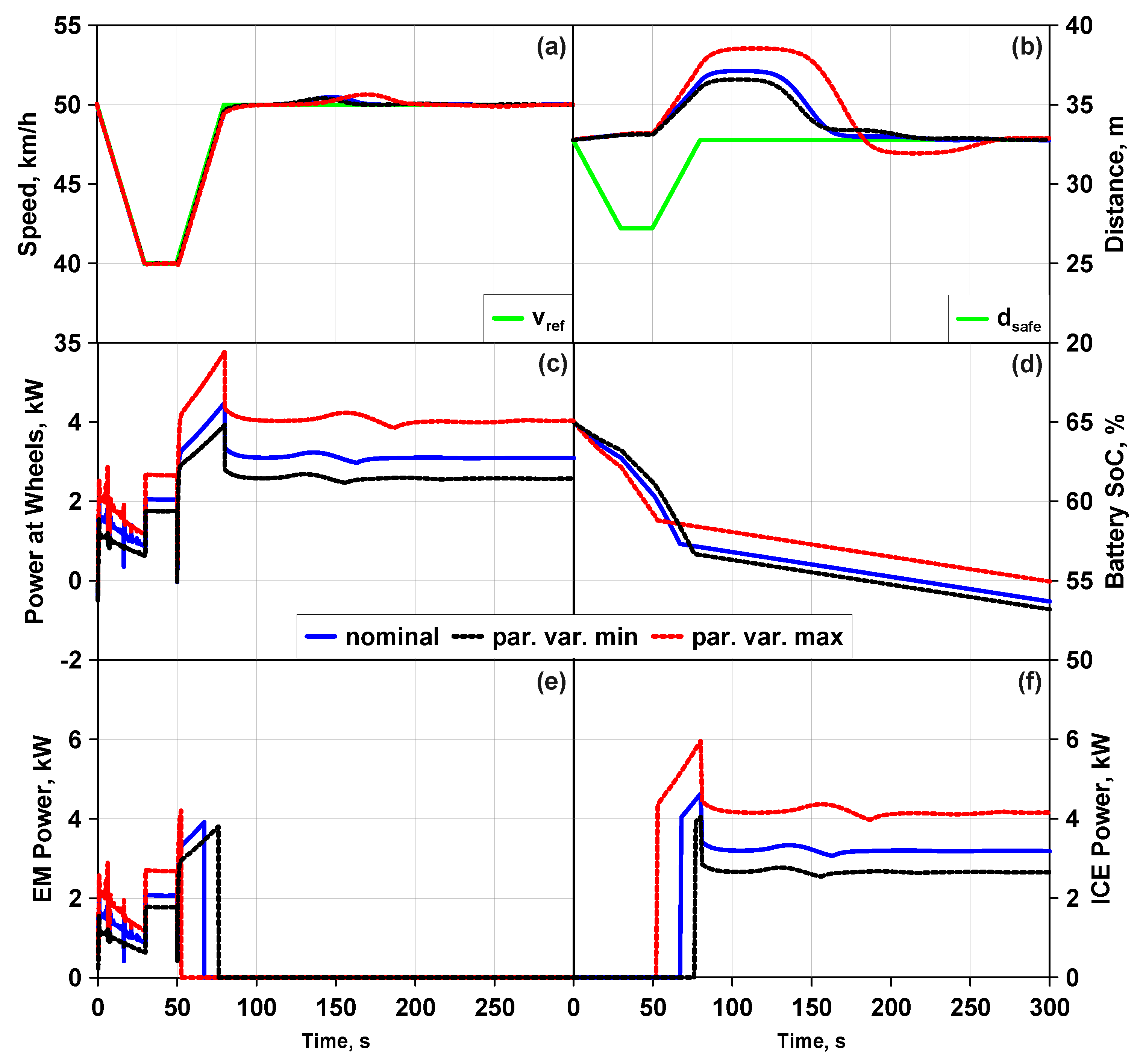
In order to check the effectiveness of the proposed controller against ego-vehicle model parameter uncertainties, robustness and sensitivity tests have been performed. Three parameters were subjected to variations: (i) drag coefficient C d ; (ii) cornering stiffness C α ; (iii) vehicle mass m. The robustness test (Figure 12 and Figure 13) shows good tracking performance for the vehicle speed and the achievement of the safety distance in the steady state. A slight deviation of about −5 mm from the nominal case in the steady state was induced by maximum parameters variations on the lateral displacement. This implies that in future developments, appropriate calibration processes should be carried out on the weights of the MPC, in order to try to improve this condition.
An additional test was performed in order to check the sensitivity of the MPC with respect to single parametric variations. The results shown in Table 8, Table 9, Table 10, Table 11, Table 12 and Table 13 show that, among the tested parameter configurations, the highest deviations from the reference are reached with the the maximum load ( m = m m a x ).
All in all, considering the RMSE index, the above variations are quite contained, except for the wheel power, which is obviously higher if the vehicle load is greater. For future developments, a calibration process on the parameters of the MPC (i.e., weights, prediction and control horizons) should be performed in order to reduce RMSE for e 1 , v x and d r for the full load condition. The cornering stiffness specifically influences some variables, that are lateral displacement e 1 and wheel power. The variation of C α determines RMSE to be quite contained, slightly affecting the steady state error. Eventually, the variations of the drag coefficient C d affect the wheel power more significantly.
At the current state, the present work is part of the research project named “Borgo 4.0”. This project has the ambitious objective, by the end of 2023, to test cooperative driving and energy management strategies in the real environment of Lioni, a small town in the province of Avellino (south Italy). In particular, the tasks of the authors on the aforementioned research project, in collaboration with NetCom Engineering S.p.A. [49], will regard the development of advanced control strategies for motion planning and energy management (on HEVs and EVs) to be tested in real-scenarios, such as:
  • Awareness driving;
  • Intersection management;
  • Rear-end collisions;
  • Long distance travels for HEVs and EVs by using benefit of Smart Road and C-ITS services.
Furthermore, NetCom Engineering has to develop an IoT gateway enabling the real communication with the Smart Road infrastructure, providing V2V, V2I and I2V communications. Thus, the selected MCU can be a hardware module of the aforementioned gateway.
Of course, a subsequent development will involve the validation of the selected MCU, using more advanced testing techniques, such as HIL with real-time simulators, and real communication channels (e.g., cellular, DSRC). In this context, the possibility to adopt a more powerful MCU will be considered. However, the advantage of this strategy has been also its development by model-based-design approach. In this way, even if future developments will require a different MCU, the control algorithm and the correspondent Simulink modules will not require substantial modifications, since only a different code generation will be requested (i.e., a different embedded coder or the same one used in this work, but applied to a more powerful STMicroelectronics MCU).
For this reason, the presented approach is general and can be extended for future developments, also considering any kind of vehicle and powertrain.

6. Conclusions

The proposed MPC featured as an intermediate layer between vehicle powertrain and Smart Road. The MPC was integrated with an energy management strategy named ETESS in order to allow, simultaneously, both motion and powertrain controls.
The Smart Road and V2V/V2I/I2V information (i.e., ISA, wind velocity, road friction, air density and car-following data exchange, such as ahead vehicle speed, mass, acceleration) were assumed to be known via simulation. Thus, the objective was to demonstrate the real-time execution on a real MCU of coupled MPC and ETESS through PIL testing, in order to allow the extension of the work for further developments.
Below, the main outcomes are summarized:
  • The average execution time of MPC + ETESS on the same MCU (STM32H743ZI2) was about 3.22 ms and therefore well below the typical CAN cycle time for torque request and steering angle, which is 10 ms.
  • ETESS was 15 times faster than ECMS; thus, this encourages the implementation of further control strategies on the same MCU, in order to reach additional real-time features, such as path planning and eco-driving.
  • Along representative maneuvers, MPC showed good tracking properties of reference speed (with an error below the 0.1% in the steady state) and lane keeping (error below 1 cm for the lateral displacement and 0.025° for the yaw angle). MPC allowed us to keep a relative distance greater than the minimum safety distance during braking phases and follows the theoretical safety distance in the steady state (with an error below 0.1%).
  • The robustness of MPC against ego-vehicle model parameters uncertainties (drag coefficient, cornering stiffness and vehicle mass) showed good tracking performance of the vehicle speed v x and a slight deviation (−5 mm; the maximum allowed is equal to 35 cm) of the lateral displacement e 1 at the maximum parameters variations ( m = m m a x , C d = C d m a x , C α = C α m a x ). The ICE activation occurred, respectively, 14 s earlier (maximum parameters variations) and 9 s later (minimum parameter variations), depending on the battery discharge rate during the early stage of the maneuver.
  • The sensitivity tests of MPC against the individual variation of single parameter of the ego-vehicle model showed a relevant influence of the maximum vehicle load ( m = m m a x ) towards all variables: lateral displacement e 1 ( M A E = 1.57 , R M S E = 0.55 cm), vehicle speed v x ( M A E = 0.52 R M S E = 0.15 km/h), relative distance d r ( M A E = 2.98 , R M S E = 1.0 m) and wheels power ( M A E = 0.98 , R M S E = 0.51 kW). With the minimum cornering stiffness C d m i n , the highest impact occurred for the lateral displacement ( M A E = 1.89 , R M S E = 0.6 cm), while with the maximum one C d m a x , the highest influence was on the wheels power ( M A E = 0.73 , R M S E = 0.03 kW). The wheels power was also significantly influenced by the drag coefficient, showing a M A E = 0.53 kW and a R M S E = 0.4 kW. Considering the RMSE indices, the variations were quite contained, except for the wheels power, which, as expected, was higher if the vehicle load and drag coefficient were greater.
The implementation of MPC and ETESS through model-based-design approach allows to easily adapt the corresponding Simulink modules for other MCUs. Nevertheless, in the case of further developments, MCUs exhibiting better performances could be required and an appropriate calibration process on the MPC parameters (weights, control and prediction horizons) could be conducted to improve its robustness and sensitivity. In particular, the MPC calibration appears appropriate to reduce the 1.89 cm gap with respect to the nominal case, which has been obtained for the lateral displacement with lower tire cornering stiffness.
The next developments of this work will include the connection between the proposed integrated motion and powertrain control strategies with path planning and C-ITS services, available through V2X communication. Moreover, the HIL testing through a co-simulation environment will be performed to consider the interaction between the ego-vehicle, other vehicles and the Smart Road using real communication channels (e.g., cellular network, DSRC). The HIL testing will also be necessary to overcome the limitations of the current testing approach (PIL), which is based on asynchronous communication between a PC-Host and the selected development board (NUCLEO-H743ZI2), while allowing the verification robust execution in real-time. Through HIL test it will be possible to understand, by implementing other additional control strategies for path planning and eco-driving, whether the selected MCU can be confirmed. If it will be necessary to change MCU, by using the model-based-design approach, the implemented control modules will not change. In addition, further developments will regard the design of other strategies for motion and powertrain controls, considering, for example, the use of other MPC types, in order to compare them with the present adaptive MPC. Possible alternatives could be: robust MPC, NLMPC and Data-Driven MPC, on which there are promising studies in the literature, as in [50,51,52].
Eventually, the presented strategy is part of the research project Borgo 4.0, in partnership with NetCom Engineering. This project foresees real road test by the end of 2023, in order to verify motion, energy management, decision making and path planning strategies in different scenarios (such as intersection management, rear-end collisions and eco-driving) by using the IoT gateway that will be designed by NetCom Engineering. Thus, the selected MCU could be an hardware module of the aforementioned IoT gateway.

Author Contributions

Conceptualization, E.L., C.N. and V.D.B.; methodology, E.L., C.N., E.M. and V.D.B.; modeling and testing hybrid powertrain with ETESS and ECMS in MIL, N.M. and F.J.M.; MPC development, E.L. and C.N.; PIL validation, E.L.; writing, all authors. All authors have read and agreed to the published version of the manuscript.

Funding

This work was partially supported by Netcom Engineering S.p.A. through the research projects “C-Mobility” and “E-Mobility” (Borgo 4.0), POR Campania FESR 2014-2020.

Data Availability Statement

Data shown in Table 1 and Table 3 are available at the following link: https://drive.google.com/file/d/1N7juTYGn9KHT_YgaMwwb4V-CXrIsfIuZ/view?usp=sharing (accessed on 17 August 2021).

Conflicts of Interest

The authors declare no conflict of interest.

References

  1. Fleming, B. Automotive Safety and Convenience Electronics [Automotive Electronics]. IEEE Veh. Technol. Mag. 2008, 3, 10–40. [Google Scholar] [CrossRef]
  2. Mecocci, A.; Shahar, M.; Ericsson, P.; Piccand, S.; Ravyse, I.; Llewellyn, T.; Di Censo, D. Sensors fusion paradigm for smart interactions between driver and vehicle. In Proceedings of the 2016 IEEE SENSORS, Orlando, FL, USA, 30 October–2 November 2016; pp. 1–3. [Google Scholar]
  3. Guanetti, J.; Kim, Y.; Borrelli, F. Control of connected and automated vehicles: State of the art and future challenges. Annu. Rev. Control 2018, 45, 18–40. [Google Scholar] [CrossRef] [Green Version]
  4. Marilisa, B.; Luigi, P.; Nicola, B.G. C-ITS communication: An insight on the current research activities in the European Union. Int. J. Transp. Syst. 2018, 3, 52–63. [Google Scholar]
  5. De Bellis, V.; Malfi, E.; Tufano, D.; Bozza, F. Efficient Thermal Electric Skipping Strategy Applied to the Control of Series/Parallel Hybrid Powertrain; Technical Report; SAE International: Warrendale, PA, USA, 2020. [Google Scholar]
  6. De Bellis, V.; Malfi, E.; Zaccardi, J.M. Development of an Efficient Thermal Electric Skipping Strategy for the Management of a Series/Parallel Hybrid Powertrain. Energies 2021, 14, 889. [Google Scholar] [CrossRef]
  7. Landolfi, E.; Salvi, A.; Troiano, A.; Natale, C. Model-Based Design and Processor-in-the-Loop Validation of a Model Predictive Control for Coupled Longitudinal-Lateral Vehicle Dynamics of Connected and Automated Vehicles. In Proceedings of the 29th IEEE Mediterranean Conference on Control and Automation (MED), Puglia, Italy, 22–25 June 2021; pp. 699–705. [Google Scholar]
  8. Emara, D.; Ezzat, M.; Abdelaziz, A.Y.; Mahmoud, K.; Lehtonen, M.; Darwish, M.M. Novel Control Strategy for Enhancing Microgrid Operation Connected to Photovoltaic Generation and Energy Storage Systems. Electronics 2021, 10, 1261. [Google Scholar] [CrossRef]
  9. Elsisi, M.; Tran, M.Q.; Mahmoud, K.; Lehtonen, M.; Darwish, M.M. Robust design of ANFIS-based blade pitch controller for wind energy conversion systems against wind speed fluctuations. IEEE Access 2021, 9, 37894–37904. [Google Scholar] [CrossRef]
  10. Elsisi, M.; Mahmoud, K.; Lehtonen, M.; Darwish, M.M. Effective Nonlinear Model Predictive Control Scheme Tuned by Improved NN for Robotic Manipulators. IEEE Access 2021, 9, 64278–64290. [Google Scholar] [CrossRef]
  11. Berberich, J.; Köhler, J.; Müller, M.A.; Allgöwer, F. Robust constraint satisfaction in data-driven MPC. In Proceedings of the 2020 59th IEEE Conference on Decision and Control (CDC), Jeju Island, Korea, 14–18 December 2020; pp. 1260–1267. [Google Scholar]
  12. Qiu, W.; Ting, Q.; Shuyou, Y.; Hongyan, G.; Hong, C. Autonomous vehicle longitudinal following control based on model predictive control. In Proceedings of the 2015 34th IEEE Chinese Control Conference (CCC), Hangzhou, China, 28–30 July 2015; pp. 8126–8131. [Google Scholar]
  13. Fan, H.; Zhang, Y.; Wang, X. Longitudinal dynamics modeling and MPC strategy for high-speed supercavitating vehicles. In Proceedings of the 2011 IEEE International Conference on Electric Information and Control Engineering, Yichang, China, 16–18 September 2011; pp. 5947–5950. [Google Scholar]
  14. Bujarbaruah, M.; Zhang, X.; Tseng, H.E.; Borrelli, F. Adaptive MPC for autonomous lane keeping. arXiv 2018, arXiv:1806.04335. [Google Scholar]
  15. Palmieri, G.; Barbarisi, O.; Scala, S.; Glielmo, L. An integrated LTV-MPC lateral vehicle dynamics control: Simulation results. In Automotive Model Predictive Control; Springer: Berlin/Heidelberg, Germany, 2010; pp. 231–255. [Google Scholar]
  16. Vyas, M. Trends of FPGA use in Automotive Engineering. In Proceedings of the 2018 3rd IEEE International Conference on Recent Trends in Electronics, Information & Communication Technology (RTEICT), Bangalore, India, 18–19 May 2018; pp. 580–591. [Google Scholar]
  17. Martín Soroa, I.; Ibrahim, A.; Goswami, D.; Li, H. Feasibility study and benchmarking of embedded MPC for vehicle platoons. In Workshop on Autonomous Systems Design (ASD 2019); Schloss Dagstuhl-Leibniz-Zentrum fuer Informatik: Wadern, Germany, 2019. [Google Scholar]
  18. Baunach, M.; Gomes, R.M.; Malenko, M.; Mauroner, F.; Ribeiro, L.B.; Scheipel, T. Smart mobility of the future—A challenge for embedded automotive systems. e & i Elektrotechnik Informationstechnik 2018, 135, 304–308. [Google Scholar]
  19. ARM-Automotive. A Starter’s Guide to Arm Processing Power in Automotive. Available online: https://armkeil.blob.core.windows.net/developer/Files/pdf/guide/starters-guide-to-arm-processing-power-in-automotive.pdf (accessed on 1 April 2021).
  20. ST Microelectronics. STM32H7 Nucleo-144 Boards (MB1364); ST Microelectronics: Santa Clara, CA, USA, 2020. [Google Scholar]
  21. ST Microelectronics. STM32 Embedded Target for MATLAB and Simulink with PIL and External Mode Processing (RN0087). Available online: https://www.st.com/en/development-tools/stm32-mat-target.html (accessed on 1 April 2021).
  22. Delprat, S.; Lauber, J.; Guerra, T.M.; Rimaux, J. Control of a parallel hybrid powertrain: Optimal control. IEEE Trans. Veh. Technol. 2004, 53, 872–881. [Google Scholar] [CrossRef]
  23. Barsali, S.; Miulli, C.; Possenti, A. A control strategy to minimize fuel consumption of series hybrid electric vehicles. IEEE Trans. Energy Convers. 2004, 19, 187–195. [Google Scholar] [CrossRef]
  24. Kim, N.; Cha, S.; Peng, H. Optimal control of hybrid electric vehicles based on Pontryagin’s minimum principle. IEEE Trans. Control Syst. Technol. 2010, 19, 1279–1287. [Google Scholar]
  25. Patil, R.M.; Filipi, Z.; Fathy, H.K. Comparison of supervisory control strategies for series plug-in hybrid electric vehicle powertrains through dynamic programming. IEEE Trans. Control Syst. Technol. 2013, 22, 502–509. [Google Scholar] [CrossRef]
  26. Paganelli, G.; Delprat, S.; Guerra, T.M.; Rimaux, J.; Santin, J.J. Equivalent consumption minimization strategy for parallel hybrid powertrains. In Proceedings of the Vehicular Technology Conference, IEEE 55th Vehicular Technology Conference, VTC Spring 2002 (Cat. No. 02CH37367), Birmingham, AL, USA, 6–9 May 2002; Volume 4, pp. 2076–2081. [Google Scholar]
  27. Sun, C.; Sun, F.; He, H. Investigating adaptive-ECMS with velocity forecast ability for hybrid electric vehicles. Appl. Energy 2017, 185, 1644–1653. [Google Scholar] [CrossRef]
  28. Shi, D.; Liu, S.; Cai, Y.; Wang, S.; Li, H.; Chen, L. Pontryagin’s minimum principle based fuzzy adaptive energy management for hybrid electric vehicle using real-time traffic information. Appl. Energy 2021, 286, 116467. [Google Scholar] [CrossRef]
  29. Biswas, A.; Emadi, A. Energy management systems for electrified powertrains: State-of-the-art review and future trends. IEEE Trans. Veh. Technol. 2019, 68, 6453–6467. [Google Scholar] [CrossRef]
  30. Zhang, F.; Hu, X.; Langari, R.; Cao, D. Energy management strategies of connected HEVs and PHEVs: Recent progress and outlook. Prog. Energy Combust. Sci. 2019, 73, 235–256. [Google Scholar] [CrossRef]
  31. Hu, X.; Zhang, X.; Tang, X.; Lin, X. Model predictive control of hybrid electric vehicles for fuel economy, emission reductions, and inter-vehicle safety in car-following scenarios. Energy 2020, 196, 117101. [Google Scholar] [CrossRef]
  32. Liu, H.; Li, X.; Wang, W.; Wang, Y.; Han, L.; Wei, W. Energy management strategy based on gis information and mpc for a heavy-duty dual-mode power-split HEV. In Proceedings of the 2018 3rd IEEE International Conference on Advanced Robotics and Mechatronics (ICARM), Sigapore, 18–20 July 2018; pp. 380–385. [Google Scholar]
  33. Chebly, A. Trajectory Planning and Tracking for Autonomous Vehicles Navigation. Ph.D. Thesis, Université de Technologie de Compiègne, Compiègne, France, 2017. [Google Scholar]
  34. Rajamani, R. Vehicle Dynamics and Control; Springer Science & Business Media: Berlin/Heidelberg, Germany, 2011. [Google Scholar]
  35. Falcone, P.; Borrelli, F.; Asgari, J.; Tseng, H.E.; Hrovat, D. Predictive active steering control for autonomous vehicle systems. IEEE Trans. Control Syst. Technol. 2007, 15, 566–580. [Google Scholar] [CrossRef]
  36. Shakouri, P.; Ordys, A.; Askari, M.; Laila, D.S. Longitudinal vehicle dynamics using Simulink/Matlab. In UKACC International Conference on Control 2010; IET: London, UK, 2010; pp. 1–6. [Google Scholar]
  37. Bolzern, P.G.E.; Scattolini, R.; Schiavoni, N.L. Fondamenti di Controlli Automatici; McGraw-Hill: New York, NY, USA, 2008. [Google Scholar]
  38. Wang, L. Model Predictive Control System Design and Implementation Using MATLAB®; Springer Science & Business Media: Berlin/Heidelberg, Germany, 2009. [Google Scholar]
  39. Satzger, C.; De Castro, R. Combined wheel-slip control and torque blending using MPC. In Proceedings of the 2014 IEEE International Conference on Connected Vehicles and Expo (ICCVE), Vienna, Austria, 3–7 November 2014; pp. 618–624. [Google Scholar]
  40. Lam, V.T.T.; Sattar, A.; Wang, L.; Lazar, M. Fast Hildreth-based Model Predictive Control of Roll Angle for a Fixed-Wing UAV. IFAC-PapersOnLine 2020, 53, 5757–5763. [Google Scholar] [CrossRef]
  41. Jin, X.; Liu, K.; Feng, Y.; Huang, Y.; Zhao, Y.; Cui, S.; Yuan, G. Motion control of thruster-driven underwater vehicle based on Model Predictive Control. In Proceedings of the 2016 IEEE International Conference on Cyber Technology in Automation, Control, and Intelligent Systems (CYBER), Chengdu, China, 10–14 October 2016; pp. 512–517. [Google Scholar]
  42. Al-Gabalawy, M.; Mahmoud, K.; Darwish, M.M.; Dawson, J.A.; Lehtonen, M.; Hosny, N.S. Reliable and Robust Observer for Simultaneously Estimating State-of-Charge and State-of-Health of LiFePO4 Batteries. Appl. Sci. 2021, 11, 3609. [Google Scholar] [CrossRef]
  43. Minervini, N. ECMS Implementation for a Hybrid Powertrain Integrated into an Autonomous and Connected Vehicle. Master’s Thesis, University of Naples Federico II, Portici, Italy, 2021. [Google Scholar]
  44. Minervini, F. ETESS for the Energy Management of the Hybrid Powertrain in an Autonomous and Connected Vehicle. Master’s Thesis, University of Naples Federico II, Portici, Italy, 2021. [Google Scholar]
  45. Sandmann, G.; Thompson, R. Development of AUTOSAR software components within model-based design. Development 2008, 1, 0383. [Google Scholar]
  46. Ficek, C.; Feiertag, N.; Richter, K. Applying the AUTOSAR timing protection to build safe and efficient ISO 26262 mixed-criticality systems. In Proceedings of the Embedded Real Time Software and Systems (ERTS2012), Toulouse, France, 29 January–1 February 2012. hal-02192404. [Google Scholar]
  47. Layal, V. Analysis and Specification of an AUTOSAR Based ECU in Compliance with ISO 26262 Functional Safety Standard. Master’s Thesis, Technische Universität Chemnitz, Chemnitz, Germany, 2016. [Google Scholar]
  48. MOUSER Electronics. Available online: https://eu.mouser.com/ (accessed on 17 August 2021).
  49. NetCom Engineering S.p.A. Available online: https://www.netcomgroup.eu/ (accessed on 17 August 2021).
  50. Zhang, W. A robust lateral tracking control strategy for autonomous driving vehicles. Mech. Syst. Signal Process. 2021, 150, 107238. [Google Scholar] [CrossRef]
  51. Rosolia, U.; Braghin, F.; Sabbioni, E.; Alleyne, A.; De Bruyne, S. A Cooperative Driving NLMPC for Real Time Collision Avoidance. In International Design Engineering Technical Conferences and Computers and Information in Engineering Conference; American Society of Mechanical Engineers: New York, NY, USA, 2015; Volume 57106, p. V003T01A015. [Google Scholar]
  52. Rosolia, U.; Zhang, X.; Borrelli, F. Data-driven predictive control for autonomous systems. Annu. Rev. Control Robot. Auton. Syst. 2018, 1, 259–286. [Google Scholar] [CrossRef]
Figure 1. Errors with respect to the road.
Wevj 12 00159 g001
Figure 2. Car following.
Wevj 12 00159 g002
Figure 3. Adaptive MPC flow chart for model-based design approach.
Wevj 12 00159 g003
Figure 4. Hybrid powertrain configuration.
Wevj 12 00159 g004
Figure 5. Flowchart schematizing the logic of ETESS.
Wevj 12 00159 g005
Figure 6. (a) Target speed (km/h). (b) Battery SoC (%) between ETESS and ECMS. (c) Power split between ETESS and ECMS.
Wevj 12 00159 g006
Figure 7. Power (kW) comparison between ETESS and ECMS: (a) ICE; (b) EM; (c) EG.
Wevj 12 00159 g007
Figure 8. Block scheme for PIL testing.
Wevj 12 00159 g008
Figure 9. Test case 1: (a) speed (km/h); (b) relative distance (m); (c) ICE/EM/Wheels power (kW); (d) battery SoC (%).
Wevj 12 00159 g009
Figure 10. Test case 2: (a) lateral displacement (m); (b) yaw angle error (deg); (c) steering angle at the wheels (deg); (d) road curvature (m−1).
Wevj 12 00159 g010
Figure 11. Test case 2: (a) speed (km/h); (b) relative distance (m); (c) ICE/EM/Wheels power (kW); (d) battery SoC (%).
Wevj 12 00159 g011
Figure 12. Robustness test (blue: nominal values, dashed red: maximum values, dashed black: minimum values)—(a) lateral displacement (m); (b) yaw angle error (deg); (c) steering angle at the wheels (deg); (d) road curvature (m−1).
Wevj 12 00159 g012
Figure 13. Robustness test (blue: nominal values, dashed red: maximum values, dashed black: minimum values)—(a) speed (km/h); (b) relative distance (m); (c) wheel power (kW); (d) battery SoC (%); (e) EM power (kW); (f) ICE power (kW).
Wevj 12 00159 g013
Figure 14. Sensitivity test (blue: nominal case (m), dashed red: maximum case ( m m a x ), dashed black: minimum case ( m m i n )) with parametric variations on vehicle mass—(a) speed (km/h); (b) relative distance (m); (c) wheels power (kW); (d) battery SoC (%); (e) EM power (kW); (f) ICE power (kW).
Wevj 12 00159 g014
Table 1. Parameters of the ego-vehicle model.
ParameterDescriptionDescription
mVehicle mass1055 kg
R e f f Effective wheel radius0.29 m
0.5 ρ A C d Aerodynamic force coefficient0.503 kg/m
LVehicle length3.571 m
T h Reaction time for safety distance evaluation2 s
I w Moment of inertia of the wheels1.85 kgm2
I z Yaw moment of inertia1338.2 kgm2
L f Dist. vehicle’s CoG to front wheel axis1 m
L r Dist. vehicle’s CoG to rear wheel axis1.3 m
C α Longitudinal tire stiffness67,689 N/rad
τ m a x Maximum wheel torque664 Nm
τ m i n Maximum braking torque at the wheel−850 Nm
δ m a x Maximum steering angle at the wheel
δ m i n Minimum steering angle at the wheel−3°
τ b s Braking phase time constant0.2 s
K b Gain for braking system14
K c Gain for pressure of brake1
v w Wind velocity0.55 m/s
θ Slope angle0 rad
t s Simulation time1 ms
Δ t Sampling time10 ms
Table 2. Driving modes and clutch positions.
Driving ModeClutch 1Clutch 2Clutch 3
Brakingxx
Pure electric drivingxx
Pure thermal engine drivingxx
Hybrid parallel drivingx
Battery charging in series modex
Battery charging in parallel mode
Table 3. Powertrain and driveline main data.
ParameterDescriptionValue
V (cm 3 )Engine displacement999
ρ o Geometric compression ratio10.5:1
B (mm)Cylinder bore70
s (mm)Cylinder stroke80.5
nNumber of cylinders3
vNumber of valves6
P m a x _ I C E (kW)Maximum engine power51
T m a x _ I C E (Nm)Maximum engine torque92
N G B 1 Number of gear ratios of G B 1 6
η G B 1 ICE gear efficiency0.97
η D i f f Final-drive ratio efficiency1
P m a x _ E M (kW)Maximum electric motor power67.35
T m a x _ E M (Nm)Maximum electric motor torque165
N G B 2 Number of gear ratios of G B 2 2
η G B 2 EM gear efficiency0.99
P m a x _ E G (kW)Maximum electric generator power59.01
T m a x _ E G (Nm)Maximum electric generator torque240
N G B 3 Number of gear ratios of G B 3 1
η G B 3 EG gear efficiency1
R b a t ( Ω ) Battery internal resistance0.375
V b a t (V)Battery voltage400
Q m a x (Ah)Battery capacity1.78
S o C r a n g e (%)Battery SoC limits 20 ÷ 90
η P C Efficiency of the power converter0.92
Table 4. Comparison between the fuel consumption by ETESS and ECMS along three type-approval driving cycles.
Fuel Consumption (l/100 km)WLTCNEDCFTP-75
ECMS4.183.693.24
ETESS4.183.713.24
Difference (%)+0.0+0.5+0.0
Table 5. Comparison between the computational time (in MIL testing) of ETESS and ECMS along three type-approval driving cycles.
Computational Time ( s ) WLTCNEDCFTP-75
ECMS678.09440.22710.18
ETESS52.4635.0552.87
Difference (%)−92.26−92.04−92.55
Table 6. PIL testing results in the worst test case.
TaskMPCETESSECMS
Maximum CPU Utilization (%)31.900.407.93
Average CPU Utilization (%)30.300.365.36
Maximum Execution Time (ms)3.1860.040.79
Average Execution Time (ms)3.0310.0350.530
Table 7. Parametric variations of the ego-vehicle model.
ParameterMin. ValueNominal ValueMax. Value
Drag coefficient0.224 ( C d m i n )0.320 ( C d )0.416 ( C d m a x )
Vehicle mass (kg)1023 ( m m i n )1050 (m)1371 ( m m a x )
Cornering Stiffness (N/rad)34,878.9 C α m i n 49,827.0 ( C α )64,775.1 ( C α m a x )
Table 8. MAE and RMSE for e 1 .
Test CaseMAE (cm)RMSE (cm)
m = m m a x 1.57300.5498
m = m m i n 0.26810.0771
C d = C d m a x 0.10000.0977
C d = C d m i n 0.10050.0981
C α = C α m a x 1.10730.2007
C α = C α m i n 1.88630.6208
Table 9. MAE and RMSE for e 2 .
Test CaseMAE (deg)RMSE (deg)
m = m m a x 0.01480.0010
m = m m i n 0.00270.0002
C d = C d m a x 0.00070.0001
C d = C d m i n 0.00070.0001
C α = C α m a x 0.01160.0008
C α = C α m i n 0.01690.0011
Table 10. MAE and RMSE for v x .
Test CaseMAE (km/h)RMSE (km/h)
m = m m a x 0.52030.1476
m = m m i n 0.11520.0261
C d = C d m a x 0.15340.0407
C d = C d m i n 0.14300.0364
C α = C α m a x 0.03430.0040
C α = C α m i n 0.03740.0060
Table 11. MAE and RMSE for d r .
Test CaseMAE (m)RMSE (m)
m = m m a x 2.981.03
m = m m i n 0.460.15
C d = C d m a x 0.470.28
C d = C d m i n 0.470.26
C α = C α m a x 0.060.04
C α = C α m i n 0.110.07
Table 12. MAE and RMSE for wheel power.
Test CaseMAE (kW)RMSE (kW)
m = m m a x 0.980.51
m = m m i n 0.580.09
C d = C d m a x 0.530.40
C d = C d m i n 0.530.41
C α = C α m a x 0.730.03
C α = C α m i n 0.550.02
Table 13. MAE and RMSE for δ .
Test CaseMAE (deg)RMSE (deg)
m = m m a x 0.01050.0019
m = m m i n 0.00180.003
C d = C d m a x 0.00020.0000
C d = C d m i n 0.00020.0000
C α = C α m a x 0.00750.0014
C α = C α m i n 0.01390.0025
Publisher’s Note: MDPI stays neutral with regard to jurisdictional claims in published maps and institutional affiliations.

