Article

Temperature Prediction of PMSMs Using Pseudo-Siamese Nested LSTM

1
School of Information and Electronic Engineering, Zhejiang University of Science and Technology, Hangzhou 310023, China
2
College of Computer Science and Technology, Zhejiang University of Technology, Hangzhou 310014, China
3
School of Economics, Zhejiang University of Technology, Hangzhou 310014, China
*
Author to whom correspondence should be addressed.
World Electr. Veh. J. 2021, 12(2), 57; https://doi.org/10.3390/wevj12020057
Submission received: 17 February 2021 / Revised: 9 March 2021 / Accepted: 30 March 2021 / Published: 2 April 2021

Abstract

:
Permanent Magnet Synchronous Motors (PMSMs) are widely used in electric vehicles due to their simple structure, small size, and high power-density. The research on the temperature monitoring of the PMSMs, which is one of the critical technologies to ensure the operation of PMSMs, has been the focus. A Pseudo-Siamese Nested LSTM (PSNLSTM) model is proposed to predict the temperature of the PMSMs. It takes the features closely related to the temperature of PMSMs as input and realizes the temperature prediction of stator yoke, stator tooth, and stator winding. An optimization algorithm of learning rate combined with gradual warmup and decay is proposed to accelerate the convergence during the training and improve the training performance of the model. Experimental results reveal the proposed method and Nested LSTM (NLSTM) achieves high accuracy by comparing with other intelligent prediction methods. Moreover, the proposed method is slightly better than NLSTM in temperature prediction of PMSMS.

1. Introduction

Permanent magnet synchronous motors (PMSMs) are the core components of electric vehicles due to their excellent power density, efficiency, and prime torque [1]. However, the high power density will cause a serious temperature increase, which may affect the working efficiency and even damage the core components of motors [2]. Therefore, an enormous amount of research effort goes into the temperature prediction of the PMSMs to ensure the safe running of the motors [3,4].
There were three main categories of methods proposed by previous researchers to predict the temperature of PMSMs as follows: temperature formula, parameter identification, and thermal networks. Methods of the first category mainly included finite element analysis (FEA) and computational fluid dynamics (CFD) [5,6]. The advantages of these methods are convenient to obtain the temperature of arbitrarily shaped devices. However, the modeling process of these methods requires high computing complexity [7]. Methods of parameter identification were mainly realized by flux observation and signal injection [8,9], which required high precision of the measuring instruments [10]. Lumped parameter thermal networks (LPTNs) were widely used when methods of thermal networks were considered [11,12,13]. Based on the idea of the thermal circuit method, the LTPN method makes a more detailed partition of motor structure. Depending on the degree of dispersion of the topology, the thermal network can be composed of several or even hundreds of nodes. The more discrete the LTPNs are, the more accurate the result will be. However, it will also bring additional calculations.
With the rapid development of artificial intelligence technology, deep learning models have been widely applied to temperature prediction in industrial fields. Several models based on deep learning were applied to predict the environmental changes such as the greenhouse and the temperature of sea surface [14]. A long short-term memory (LSTM) network [15] was first introduced to predict the temperature of PMSMs, and it performed well in the prediction accuracy [16]. The work presented in [17] showed the feasibility of the deep residual convolutional loop network in the application of temperature prediction of PMSMs. It confirmed the feasibility and accuracy of temperature prediction of PMSMs.
The NLSTM network was another deep learning model based on the LSTM network, which owned a more efficient time hierarchy and flexible processing of internal memory [18]. It was applied to realize seizure detection combined with convolution neural networks. The advanced architecture effectively explored the inherent time dependence hidden in electroencephalogram (EEG) signals and revealed the performance as superior [19]. The ability of NLSTM to dynamically capture hierarchical time dependencies in traffic data was verified by using this characteristic. NLSTM could also efficiently access internal memory when constructing the time layer structure [20].
In this paper, a novel model based on the NLSTM called the PSNLSTM is proposed to predict the future temperature of PMSMs. Two NLSTM networks with different time steps are used to capture the time dependence and abstract features of temperature changes. Abstract features refer to higher-level features, which can better describe the temperature change characteristics of PMSMs. They are not obtained through simple linear transformations, and can be more easily learned and calculated by neural networks. Adjustment of learning rate plays a vital role in the training of the deep learning networks. Thus, an optimization algorithm of the learning rate is proposed to accelerate the convergence and improve training performance.
The remainder of this paper is organized as follows: the model of the Pseudo-Siamese NLSTM network is introduced in Section 2. The temperature benchmark of the PMSMs and evaluation indicators are introduced in Section 3. Furthermore, the optimization algorithm of the learning rate is demonstrated in Section 4. The experimental results and assessment are demonstrated in Section 5. The paper is concluded in Section 6.

2. Pseudo-Siamese Nested LSTM Network

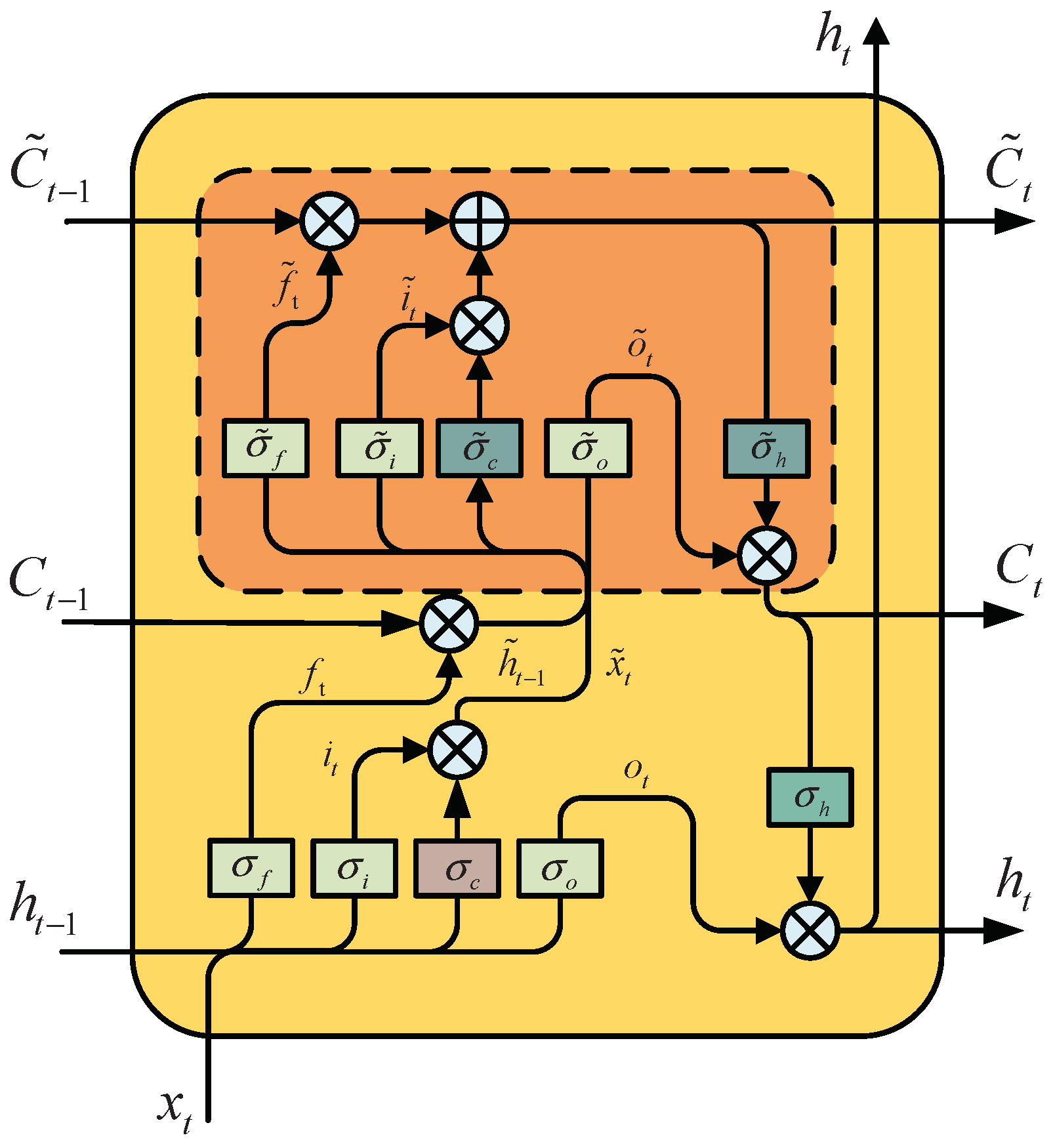
2.1. Nested LSTM Network

The NLSTM network is a novel RNN architecture with multiple levels of memories, which add depth to LSTM via nesting as opposed to stacking [18]. The architecture of the NLSTM memory block is shown in Figure 1.
The input and output of the NLSTM network are the same as the LSTM network. Another temporary cell state is added in NLSTM, which is used to transfer the memory state of the internal memory block. An NLSTM memory block is equivalent to two LSTM memory blocks in the form of a nested structure. The inner LSTM block, which is surrounded by dotted lines in Figure 1, becomes the memory function of the external LSTM block. The memory function is dedicated to managing the long-term information between the memory blocks.
The external LSTM calculates h ˜ t 1 and x ˜ t through the input x t of the current time and the output h t 1 of the previous time:
f t = σ f W f h t 1 , x t + b f
i t = σ i W i h t 1 , x t + b i
o t = σ o W o h t 1 , x t + b o
h ˜ t 1 = f t C t 1
x ˜ t = i t σ c W c x t , h t 1 + b c
where f t , i t and o t are the three states of the gates, σ i , σ ρ , σ f are the sigmoid activation functions, which realize selective memory and forgetting. They achieve long-term memory without causing a gradient explosion. σ c is the linear activation function. In addition, h ˜ t 1 and x ˜ t obtained from external LSTM are input and the hidden state of NLSTM internal memory function, respectively.
For the internal memory function, the internal operation mode is controlled by the following equation:
i ˜ t = σ ˜ i W ˜ i h ˜ t 1 , x ˜ t + b ˜ i
f ˜ t = σ ˜ f W ˜ f h ˜ t 1 , x ˜ t + b ˜ f
C ˜ t = f ˜ t C ˜ t 1 + i ˜ t σ ˜ c W ˜ c h ˜ t 1 , x ˜ + b ˜ c
o ˜ t = σ ˜ 0 W ˜ o h ˜ t 1 , x ˜ t + b ˜ o
h ˜ t = o ˜ t σ ˜ h C ˜ t
where σ ˜ i , σ ˜ o , σ ˜ f all are the sigmoid activation function, which are consistent with external LSTM. σ ˜ c , σ ˜ h are the tanh activation function. After a series of operations of the internal LSTM, the state update of the external LSTM unit is obtained:
C t = h ˜ t
Finally, the following equation is used to obtain the last output of NLSTM memory block:
h t = o t σ h C t
where σ h is the tanh activation function.

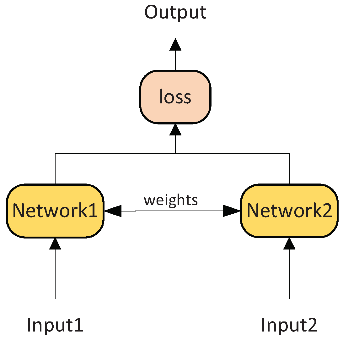
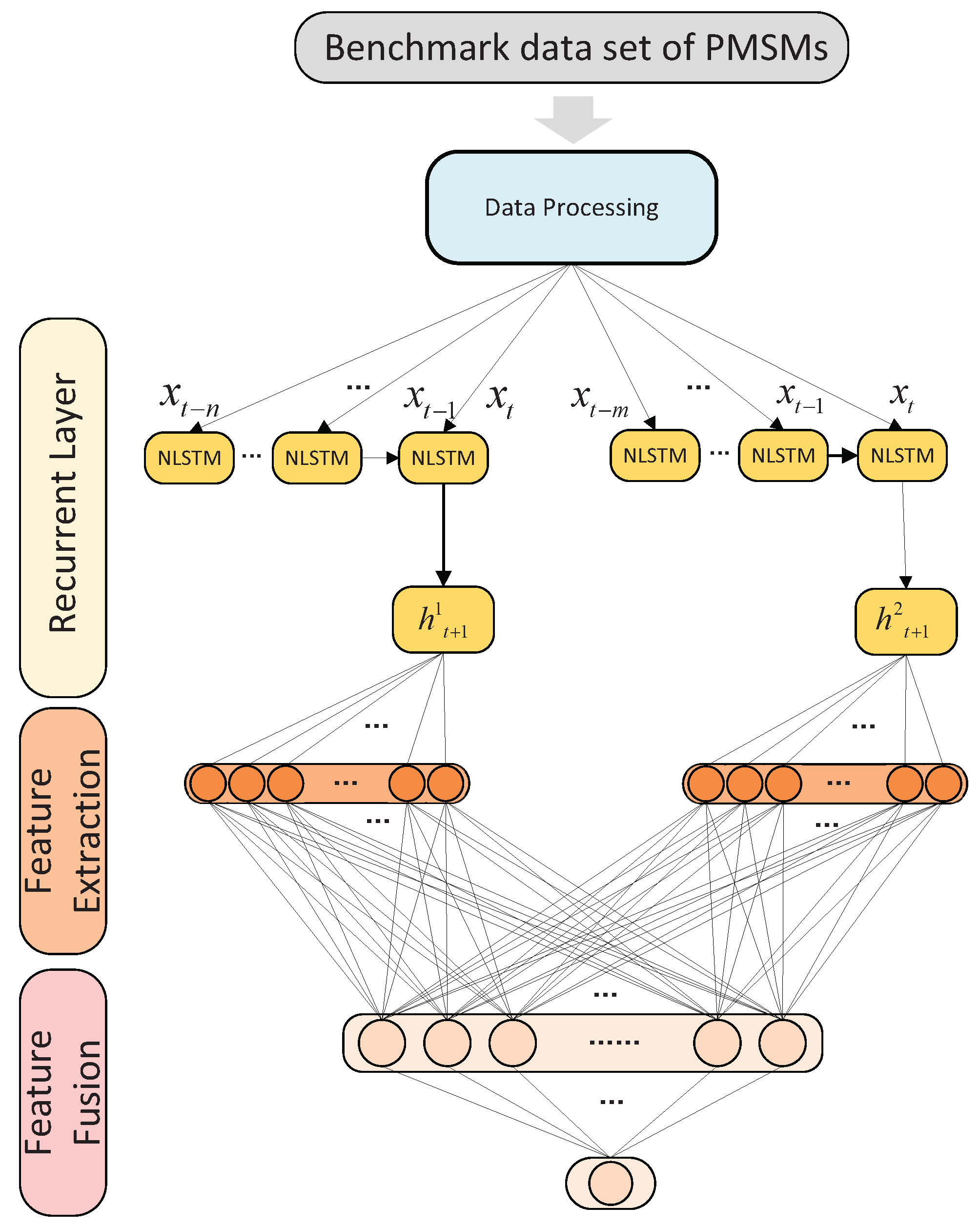
2.2. Model Architecture Proposed

The Siamese Network is a conjoined neural network architecture shown in Figure 2. It realizes “Siamese” through weight sharing [21]. If the weights of the neural networks on the left and right are not shared or the neural networks are different, the architecture is defined as the Pseudo-Siamese networks. This architecture is widely used in the fields of information similarity matching and comparison [22,23].
A novel architecture based on NLSTM and Pseudo-Siamese network calling PSNLSTM is proposed in this paper. Two NLSTM networks with different time steps are adopted as the neural networks in the Pseudo-Siamese network. The architecture of the model is shown in Figure 3. After the temperature benchmark data set of PMSMs is preprocessed, it is sent to the recurrent layer. In the recurrent layer, one NLSTM network with long time steps is used to obtain the trend of temperature series changes of PMSMs. The other with short time steps is used to obtain the detail of the temperature series changes. Through the above two NLSTM networks, the higher level temperature features of the next moment are obtained. Then, a full connection layer is added to extract the temperature features for each NLSTM network. Finally, another full connection layer is used to fuse the temperature features of different neural networks to get the predicted temperature.

3. Temperature Benchmark Data Set and Valuation Indicators

3.1. Temperature Benchmark Data Set

The data set used in this experiment is from the Kaggle Data Science online competition platform. In addition, it is based on a test bench having a three-phase PMSM mounted (for detailed information of PMSM, see [24]). The data measurement and collection are provided by the Department of Power Electronics and Electrical Drive of Paderborn University in Germany. Table 1 shows the column labels for the benchmark dataset. It includes more than 990,000 pieces of data.
All recordings are sampled at 2 Hz. Each measurement session in the data set can represent the entire electrothermal characteristics of the PMSM well. In addition, this data set is mildly anonymized, and each set of parameters has been standardized.
In the experiment, 51 measurement sessions in the entire data were set as the training set, and the one remaining session ( i d = 32 ) was set as the test set. The data set was down-sampled at an appropriate frequency and cleaned. Since each measurement session is independent of each other, the down-sampling operation is performed separately, retaining only the same frequency. In addition, from time to time in the training model, data from different measurement session is not continuous data as input to the model. Finally, the number of data in the training sets is 32,263, and the number of data in the test sets is 412.
The temperatures of ϑ S Y , ϑ S T and ϑ S W are chosen as the prediction object of the PMSMs. Since the temperature characteristics of these core components are different, we have separately trained PSNLSTM and the comparative models. In addition, the input of the model does not include the predicted target temperature feature.

3.2. Evaluation Indicators

There are several common evaluation indicators adopted to evaluate the prediction accuracy as follows: mean square error (MSE), root mean square error (RMSE), and mean absolute error (MAE). The definition formulas are as follows:
M A E = 1 n t = 0 n 1 a t p t
M S E = 1 n t = 0 n 1 a t p t 2
R M S E = 1 n t = 0 n 1 a t p t 2
Among them, a t and p t respectively represent the true value and predicted value at the time t.
To assess the volatility of the predicted results, the standard deviation of the prediction error (STDPE) is introduced, which is defined using the following formula:
d t = p t a t
S T D P E = t = 0 n 1 d t d ¯ 2 n 1
where d t is the prediction error at time t, and the definitions of the other parameters are the same as those mentioned above.
Another evaluation indicator, coefficient of determination is represented as R 2 . It can reflect the proportion of the variation of dependent variables that can be explained by independent variables, and its definition formula is as follows:
R 2 = 1 t = 0 n 1 a t p t 2 t = 0 n 1 a t a ¯ 2
It can be used to observe the prediction error compared with the mean reference error. The value region of R 2 is between 0 and 1 .

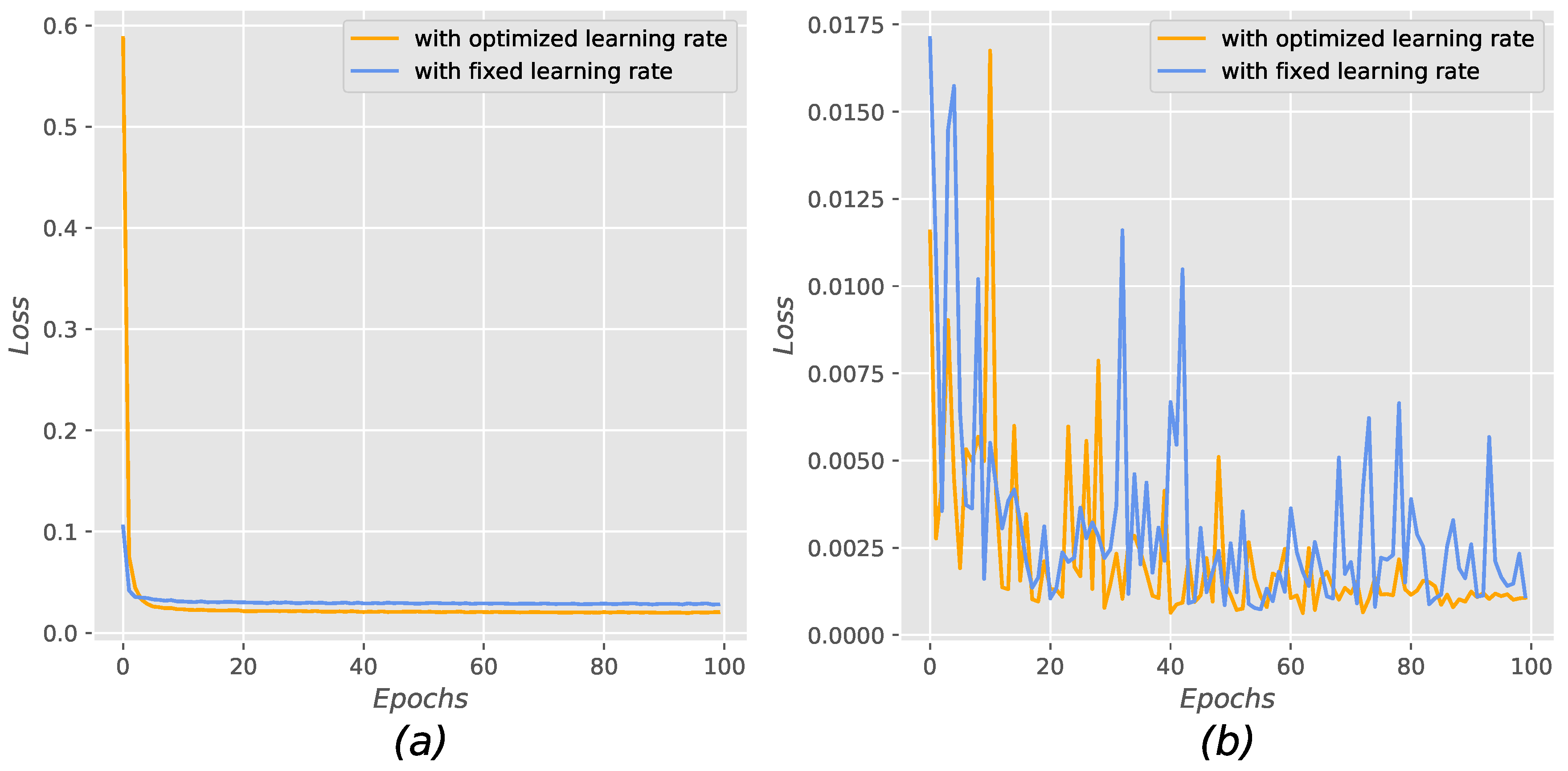
4. Learning Rate Optimization

During the training process of the deep learning models, the optimization of hyper-parameters plays an important role. As one of the essential hyper-parameters in deep learning models, the learning rate determines whether and when the objective function converges to the local optimum. A proper learning rate can help the objective function converge to an optimum in a proper period. If the value of the learning rate is too small, the loss of models will decline very slowly. Otherwise, a large learning rate will cause a considerable variation of parameters when the parameters update, which will lead to the missing of the optimal point or lead to the rise of the model loss. It is worth noting that the model requires a different learning rate in each stage of training. When the parameters fall into the local optimum, a larger learning rate is needed to escape from this point. Correspondingly, a smaller learning rate is required to approximate the global optimum.
Therefore, it is necessary to adjust the learning rate dynamically during the training of the model. Thus, gradual warmup is introduced to accelerate the convergence of deep learning models, which was first mentioned in the literature [25]. After that, the attenuation of the learning rate should be considered to get the optimal result after several epochs, instead of keeping the learning rate constant until the end. In this experiment, a novel optimization algorithm of learning rate is proposed, which combines a gradual warmup algorithm, cosine annealing algorithm, and Nadam optimizer to realize the update of the learning rate effectively. This algorithm is designed to accelerate the convergence of the NLSTM on the PMSMs temperature data set and improve its training performance.
In this optimization algorithm, the learning rate changes can be divided into the following three stages: gradual warmup, keeping constant, and annealing. First, within a certain number of training steps, the learning rate gradually increases from a small value to a preset value. Thus, the overfitting of the network can be avoided. Using a smaller learning rate can make the model gradually stabilize. After a gradual warmup, the model has achieved a relatively stable state. Then, using a larger learning rate of training, be able to make the model more quickly converge to achieve a better training effect. Second, after the gradual warmup is completed, the model will continue training at the set learning rate. It also ensures that the model can jump out of the local optimum. After that, the model result is close to the global optimum. The learning rate should be attenuated to avoid the miss of the global optimum. The cosine function is widely adopted to anneal the learning rate.
In practical applications, the combination of cosine annealing and stochastic gradient descent (SGD) can speed up model fitting to a certain extent and achieve better fitting results. Moreover, it is suggested in [26] that learning rate annealing can also be added when Adam is used. In addition, Adam [27] is different from SGD, which is an optimizer with first-order and second-order momentum. In Adam, the main parameter update formula is as follows:
θ t = θ t 1 η V ^ t + ε m ^ t = θ t 1 η V ^ t + ε β 1 m t 1 1 β 1 t + 1 β 1 g t 1 β 1 t
Among them, t is the time step of updating model parameters, θ is the parameter to be updated, β 1 is the exponential decay rate of the first-order moment, η is the learning rate, ε is the constant term, m is the first-order moment estimation of the gradient, m ^ is the correction of m, and V ^ is the correction of the second-order moment estimation of the gradient.
In this learning rate optimization algorithm, we try to use Nadam as an optimizer, which can be regarded as the combination of Nesterov and Adam [28,29]. In Nadam, the main parameter update formula is shown below:
θ t = θ t 1 η V ^ t + ε β 1 m t 1 β 1 t + 1 + 1 β 1 g t 1 β 1 t
where the definition of each parameter is the same as that of Adam. The momentum m t 1 at time t 1 is replaced by the momentum at time t , thus taking into account the “future factor” and achieving the effect of Nesterov.
To verify the proposed optimization algorithm of the learning rate, changes in the learning rate are observed in Figure 4. The fixed learning rate is set as 0.001, and the total epochs is set as 100. We define the first 10 epochs as the gradual warmup stage, the next 10 epochs as the keeping constant stage, and the rest as the cosine annealing stage.
The comparative losses of the model during the training process and validation are shown in Figure 5. We can observe that, in the first two epochs, the convergence rate of the proposed optimization algorithm is slower, which is shown in Figure 5a. Because the first 10 epochs of the optimization algorithm fall into the stage of gradual warmup and the learning rate is relatively low at the beginning, in the training set, the loss convergence performance with the optimization algorithm of learning rate is better than that without the learning rate optimization algorithm.
Figure 5b shows the validation loss curve of the proposed algorithm, which fluctuates significantly at the beginning of the epochs. In the first 10 epochs, it is in a gradual warmup stage and the learning rate increases slowly. Therefore, it fluctuates more significantly than the loss curve of the fixed learning rate. In the latter part of the epochs, it performs more stably than the loss curve with fixed leaning rate. This is due to the involvement of the cosine annealing algorithm in the later stage. After the keeping constant stage, the learning rate enters the cosine annealing stage, and its annealing according to the cosine function [0,1] interval. In the early annealing stage, the learning rate decreases slowly still remains at a large value, which helps the Nadam optimizer accumulate momentum out of the local optimal point and look for a better convergence point. Then, the learning rate gradually decreases, the model can converge quickly to the best point. Finally, the learning rate changes slowly with a small value and slowly approaches the optimal point to avoid missing it. After the above learning rate annealing, the model finally converges to a better state. Therefore, the proposed algorithm of the learning rate is helpful to accelerate the convergence and improve the accuracy of the model.

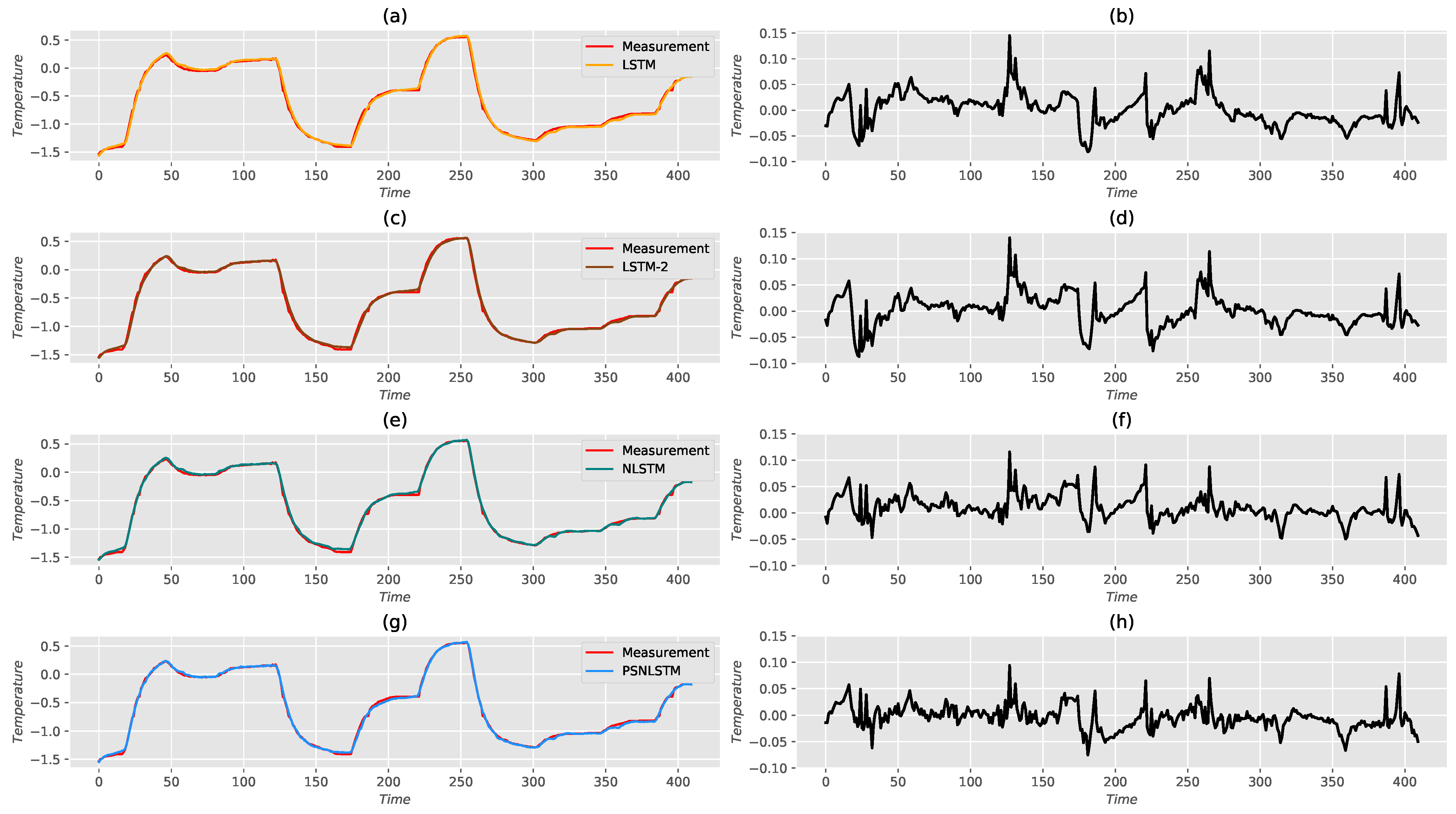
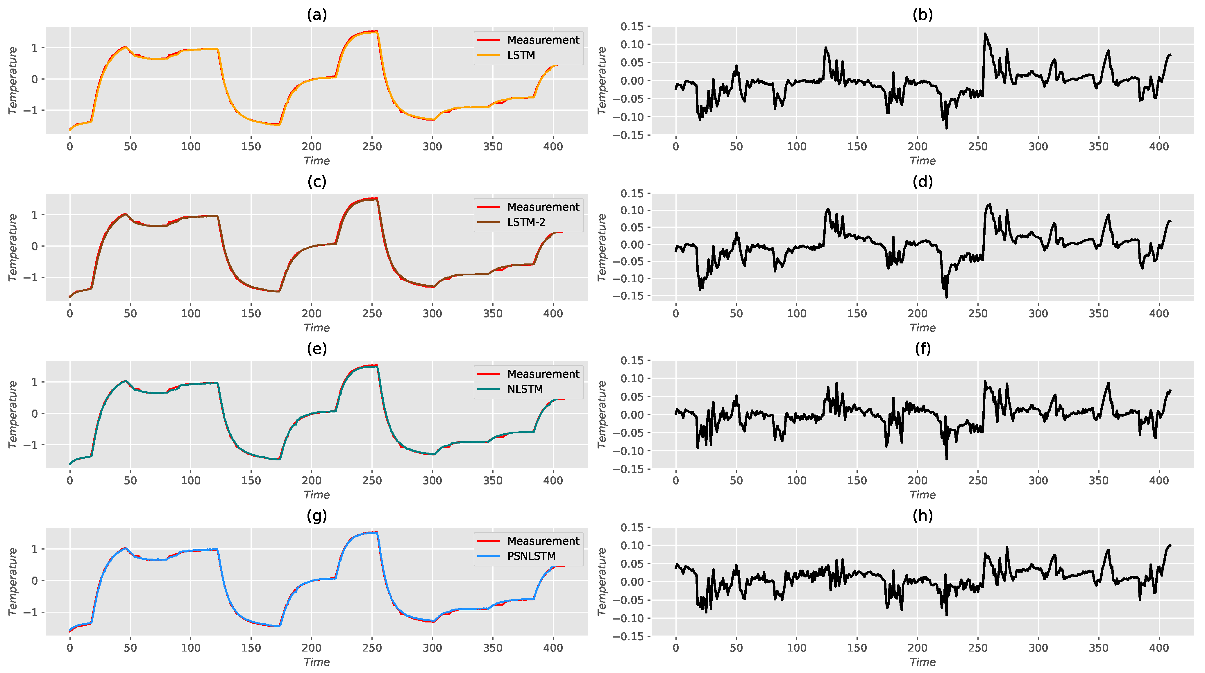
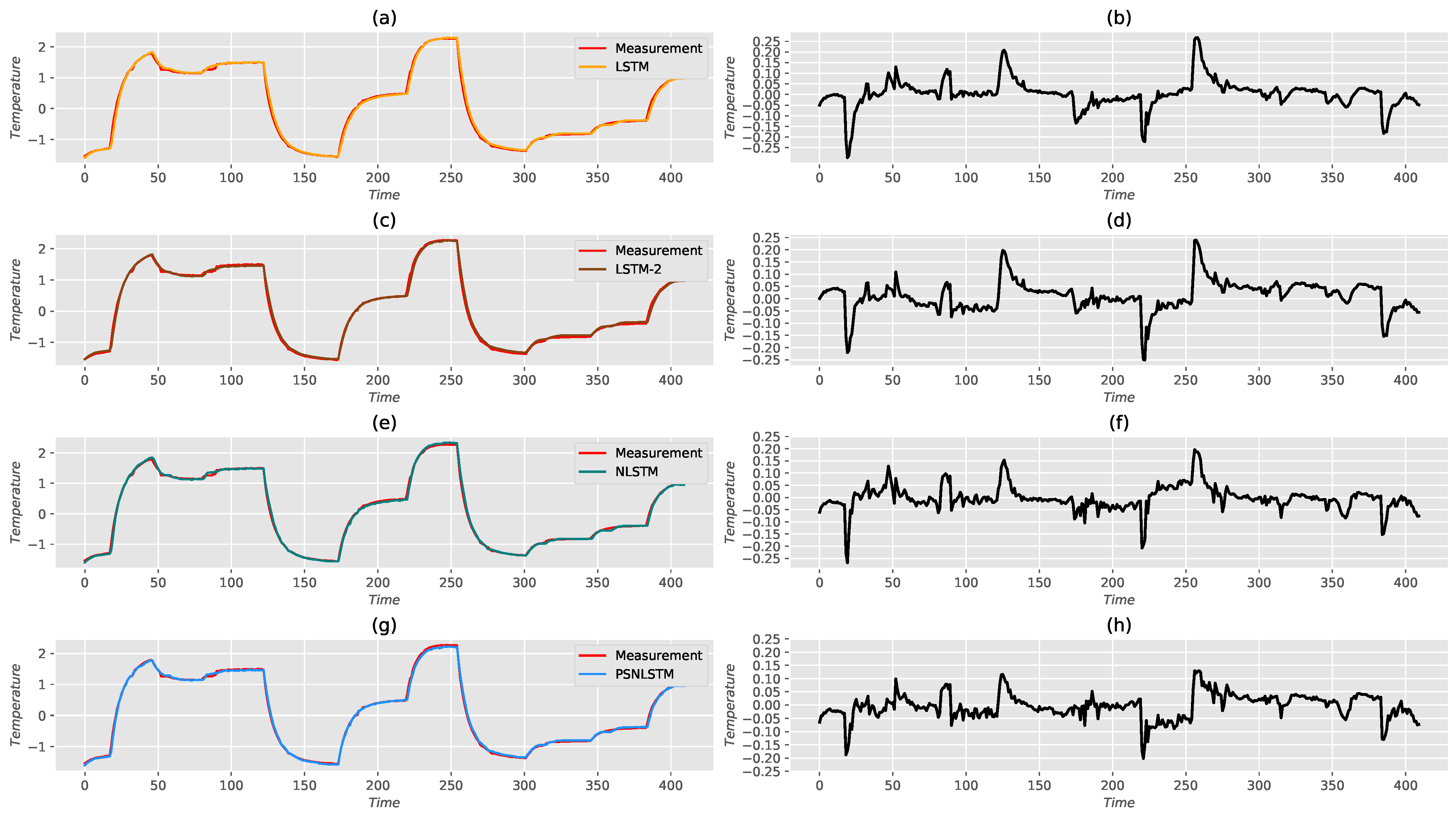
5. Performance Assessment

There are two different NLSTMs in PSNLSTM. The grid search method is used to match the lengths of time steps, then two sizes of time steps for PSNLSTM are set as 7 and 4 to obtain the different temperature features of the PMSMs. Accordingly, we set NLSTM as one of the comparative models. NLSTM is an advanced variant of LSTM, and LSTM is widely used in the prediction of temperature series. Therefore, it is necessary to compare the temperature prediction results of LSTM and PSNLSTM of PMSMs. As mentioned in Section 2.1, NLSTM is equivalent to two LSTMs which are composed of nested structures. To prove the superiority of NLSTM structure in temperature prediction of PMSM, stacked LSTM is also set as a comparative model. The stacked LSTM in this paper has two layers of LSTM network in the loop layer, called LSTM-2. In this study, LSTM, LSTM-2, NLSTM, and PSNLSTM, respectively, predict the temperature of the core components ϑ S Y , ϑ S T and ϑ S W , and all these models utilizing the temperature features at the moment t to predict the temperature at the next moment t + 1 . The time steps for the comparative models are set as 7 . The other hyper-parameters are listed in Table 2. In addition, the experiment platform is as follows: Win10 (64 bits), i7-6700HQ Intel(R)Core(TM), 16 GB, GTX960M-2G, and the versions of the deep learning framework were Keras 2.2.4 and Tensorflow 1.12.0, version of PyCharm 2020.3.2 (JetBrains, Prague, Czech Republic).
To evaluate the performance of PSNLSTM and learning rate optimization algorithm, we compare it with LSTM, LSTM-2, and NLSTM for temperature prediction of ϑ S Y , ϑ S T and ϑ S W . Table 3, Table 4 and Table 5 show the performance of each model from the four technical indicators of MSE, MAE, RMSE, R 2 , and STDPE.
The values of R 2 in Table 3, Table 4 and Table 5 for all of the models are close to 1, which means that all of these models achieve an excellent fitting effect. NLSTM performs better than LSTM in the view of R 2 because the NLSTM captures more abstract features contained in the temperature data than LSTM. The design of PSNLSTM with different time steps even creates the possibility to get more comprehensive information from the data. The NLSTM with a longer time step contains the temperature information from a longer time ago, which is conducive to learning the temperature change trend, and theoretically can reduce the prediction error of the temperature change point to a certain extent. The other NLSTM is better at learning temperature changes in a short period of time, can grasp the details of temperature changes, and theoretically can improve the accuracy of non-abrupt temperature changes to a certain extent. The values of MSE, MAE, and RMSE should be close to 0 , which reveals the good accuracy of the models. The values of MSE, MAE, and RMSE for the NLSTM are smaller compared with the LSTM and LSTM-2 in Table 3, Table 4 and Table 5. Meanwhile, the performance of PSNLSTM is better compared with the NLSTM in the temperature prediction of ϑ S W and ϑ S Y . In particular, the MSE of PSNLSTM in Table 5 is 49.82 % lower than LSTM and 43.67 % lower than LSTM-2.The performance of PSNLSTM and NLSTM are generally close for the prediction of ϑ S T . The first four evaluation indicators of PSNLSTM are slightly worse than NLSTM, but its STDPE is 8.43 % lower than that of NLSTM, that is, the prediction of PSNLSTM is more stable and its error volatility is lower. In addition, in the temperature prediction of ϑ S Y , ϑ S T and ϑ S W , the error volatility of the PSNLSTM prediction result is the lowest. In order to compare the performance difference between PSNLSTM and competitive models, the difference of the values between two networks for MSE, for MAE, for RMSE and for STDPE, respectively, and then the average of the three values is calculated. In this study, the temperatures of ϑ S Y , ϑ S T and ϑ S W were predicted, so there are three previously mentioned averages between each competitive model and PSNLSTM. Finally, the three averages are averaged, and the averages of evaluation indicators are obtained, which can describe the overall difference between each competitive model and PSNLSTM in PMSM temperature prediction. The overall error of PSNLSTM is 25.34 % lower than LSTM, 28.23 % lower than LSTM-2, and 3.68 % lower than NLSTM. The results indicate a very slight superiority of PSNLSTM over NLSTM.
The measured and predicted temperatures of the ϑ S Y and ϑ S T implemented, respectively, by LSTM, LSTM-2, NLSTM and PSNLSTM are shown in Figure 6 and Figure 7. Moreover, the prediction error curves of the models are also provided, which is calculated by Equation (16). The black error curves on the right correspond to the predictions of each model on the left.
It can be observed that the prediction temperature curves and measurement curves fit well for these four deep learning models. The fluctuation of the error curves of PSNLSTM and NLSTM, as attested visually, is less than the fluctuation of the respective curves for LSTM and LSTM-2. A less abrupt nature of the error curves is more obvious at the temperature transition time instants for both PSNLSTM and NLSTM and even a slight advantage can be attested at those time instants for PSNLSTM over NLSTM.
The measured and predicted temperatures of the ϑ S W implemented, respectively, by LSTM, LSTM-2, NLSTM, and PSNLSTM are shown in Figure 8. It can be observed that the range of error curves in Figure 8 implemented by the four models, respectively, are more extensive than in Figure 6 and Figure 7, so the temperature prediction of ϑ S W reveals difficulty. The error ranges of LSTM and LSTM-2 in Figure 8 are about 0.5 , while the error range of PSNLSTM is 0.33 . Compared with them, the advantage of PSNLSTM is obvious. Moreover, PSNLSTM has a slight advantage over NLSTM, which is mainly reflected in the sudden change points of temperature.
The performances shown in Figure 6, Figure 7 and Figure 8 are consistent with the results revealed in Table 3, Table 4 and Table 5. The weak advantage of PSNLSTM over NLSTM is mainly reflected in the mutation points of temperature, which is relatively obvious in the most difficult ϑ S W temperature prediction. To a certain extent, it supports the structural feature of PSNLSTM, which consists of two NLSTMs with different time steps. However, this structure also improves the accuracy of temperature prediction while increasing a certain amount of parameters. In this study, the temperature prediction effect for the ϑ P M component of the permanent magnet synchronous motor is not shown because the four deep learning models mentioned in the article are not ideal for the component. Both PSNLSTM and NLSTM have certain advantages over LSTM and LSTM-2 in temperature prediction. Compared with NLSTM, although PSNLSTM is slightly worse than NLSTM in ϑ S T temperature prediction, there are many slight indications that PSNLSTM was slightly better than NLSTM overall.

6. Conclusions

This paper systematically expounds on the current research on the temperature prediction of permanent magnet synchronous motors. The NLSTM, a novel deep learning model, is chosen to predict the temperature of the PMSMs. Then, the PSNLSTM, which combines the NLSTM and Pseudo-Siamese networks, is proposed. The learning rate optimization algorithm of gradual warmup and cosine annealing with the adaptive optimizer Nadam is also proposed to accelerate the convergence of the model and to improve the prediction performance. Both the proposed model and optimization algorithm of learning rate are verified by the experiments. A slight improvement is detected concerning the comparison of PSNLSTM with NLSTM, while a clear advantage of both is indicated concerning LSTM and LSTM-2. More details will be confirmed in future studies, which will include more extended datasets.

Author Contributions

Conceptualization, Y.C. (Yuefeng Cen) and G.C.; methodology, Y.C. (Yongping Cai) and Y.C. (Yuefeng Cen); formal analysis, Y.C. (Yongping Cai) and C.Z.; writing—original draft preparation, Y.C. (Yuefeng Cen) and Y.C. (Yongping Cai); writing—review and editing, X.Y., C.Z., and Y.Z.; visualization, G.C. and X.Y. All authors have read and agreed to the published version of the manuscript.

Funding

This research was funded by the National Natural Foundation of China (Grant Nos. Nsfc61902349 and Nsfc61803337).

Acknowledgments

We are grateful to the Kaggle data science competition platform and the University of Paderborn in Germany for their dataset: https://www.kaggle.com/wkirgsn/electric-motor-temperature (accessed on 1 April 2021).

Conflicts of Interest

The authors declare that there is no conflict of interest. The funders had no role in the design of the study; in the collection, analyses, or interpretation of data; in the writing of the manuscript; or in the decision to publish the results.

References

  1. Fan, T.; Li, Q.; Wen, X. Development of a High Power Density Motor Made of Amorphous Alloy Cores. IEEE Trans. Ind. Electron. 2013, 61, 4510–4518. [Google Scholar] [CrossRef]
  2. Wu, P.S.; Hsieh, M.F.; Cai, W.L.; Liu, J.H.; Huang, Y.T.; Caceres, J.F.; Chang, S.W. Heat Transfer and Thermal Management of Interior Permanent Magnet Synchronous Electric Motor. Inventions 2019, 4, 69. [Google Scholar] [CrossRef] [Green Version]
  3. Guo, H.; Ding, Q.; Song, Y.; Tang, H.; Wang, L. Predicting Temperature of Permanent Magnet Synchronous Motor Based on Deep Neural Network. Energies 2020, 13, 4782. [Google Scholar] [CrossRef]
  4. Zhu, Y.; Xiao, M.; Lu, K.; Wu, Z.; Tao, B. A simplified thermal model and online temperature estimation method of permanent magnet synchronous motors. Appl. Sci. 2019, 9, 3158. [Google Scholar] [CrossRef] [Green Version]
  5. Habibinia, D.; Rostami, N.; Feyzi, M.R.; Soltanipour, H.; Pyrhönen, J. New finite element based method for thermal analysis of axial flux interior rotor permanent magnet synchronous machine. IET Electr. Power. Appl. 2019, 14, 464–470. [Google Scholar] [CrossRef]
  6. Feng, G.; Lai, C.; Iyer, K.L.V.; Kar, N.C. Improved high-frequency voltage injection based permanent magnet temperature estimation for PMSM condition monitoring for EV applications. IEEE Trans. Appl. Supercon. 2020, 30, 1–5. [Google Scholar] [CrossRef]
  7. Boglietti, A.; Cavagnino, A.; Staton, D.; Shanel, M.; Mueller, M.; Mejuto, C. Evolution and modern approaches for thermal analysis of electrical machines. IEEE Trans. Ind. Electron. 2009, 56, 871–882. [Google Scholar] [CrossRef] [Green Version]
  8. Kral, C.; Haumer, A.; Lee, S.B. A Practical Thermal Model for the Estimation of Permanent Magnet and Stator Winding Temperatures. IEEE Trans. Veh. Technol. 2017, 67, 216–225. [Google Scholar] [CrossRef]
  9. Qiao, G.; Wang, M.; Liu, F.; Liu, Y.; Zheng, P.; Sui, Y. Analysis of Magnetic Properties of AlNiCo and Magnetization State Estimation in Variable-Flux PMSMs. IEEE Trans. Magn. 2019, 55, 1–6. [Google Scholar] [CrossRef]
  10. Wallscheid, O.; Huber, T.; Peters, W.; Böcker, J. A critical review of techniques to determine the magnet temperature of permanent magnet synchronous motors under real-time conditions. EPE J. 2016, 26, 11–20. [Google Scholar] [CrossRef]
  11. Balamurali, A.; Kundu, A.; Clandfield, W.; Kar, N.C. Non–invasive parameter and loss determination in PMSM considering the effects of saturation, cross–saturation, time harmonics and temperature variations. IEEE Trans. Magn. 2020, 57, 8202206. [Google Scholar]
  12. Giangrande, P.; Madonna, V.; Nuzzo, S.; Spagnolo, C.; Gerada, C.; Galea, M. Reduced Order Lumped Parameter Thermal Network for Dual Three-Phase Permanent Magnet Machines. In Proceedings of the 2019 IEEE Workshop on Electrical Machines Design, Control and Diagnosis (WEMDCD), Athens, Greece, 22–23 April 2019; pp. 71–76. [Google Scholar]
  13. Rostami, N.; Feyzi, M.R.; Pyrhonen, J.; Parviainen, A.; Niemela, M. Lumped-parameter thermal model for axial flux permanent magnet machines. IEEE. Trans. Electr. Power. Appl. 2017, 49, 1178–1184. [Google Scholar] [CrossRef]
  14. Yu, X.; Shi, S.; Xu, L.; Liu, Y.; Miao, Q.; Sun, M. A Novel Method for Sea Surface Temperature Prediction Based on Deep Learning. Math. Probl. Eng. 2020, 2020, 1–9. [Google Scholar] [CrossRef]
  15. Hochreiter, S. The vanishing gradient problem during learning recurrent neural nets and problem solutions. Int. J. Uncertain. Fuzz. 1998, 6, 107–116. [Google Scholar] [CrossRef] [Green Version]
  16. Wallscheid, O.; Kirchgässner, W.; Böcker, J. Investigation of long short-term memory networks to temperature prediction for permanent magnet synchronous motors. In Proceedings of the 2017 International Joint Conference On Neural Networks (IJCNN), Anchorage, AK, USA, 14–19 May 2017; pp. 1940–1947. [Google Scholar]
  17. Kirchgässner, W.; Wallscheid, O.; Böcker, J. Deep residual convolutional and recurrent neural networks for temperature estimation in permanent magnet synchronous motors. In Proceedings of the 2019 IEEE International Electric Machines and Drives Conference (IEMDC), San Diego, CA, USA, 11–15 May 2019; pp. 1439–1446. [Google Scholar]
  18. Moniz, J.R.A.; Krueger, D. Nested lstms. In Proceedings of the Ninth Asian Conference on Machine Learning (ACML2017), Seoul, Korea, 15–17 November 2017; pp. 15–17. [Google Scholar]
  19. Li, Y.; Yu, Z.; Chen, Y.; Yang, C.; Li, Y.; Allen, L.X.; Li, B. Automatic Seizure Detection using Fully Convolutional Nested LSTM. Int. J. Neural Syst. 2020, 30, 2050019. [Google Scholar] [CrossRef]
  20. Ma, X.; Zhong, H.; Li, Y.; Ma, J.; Cui, Z.; Wang, Y. Forecasting transportation network speed using deep capsule networks with nested lstm models. IEEE Trans. Intell. Transp. 2020, 99, 1–12. [Google Scholar] [CrossRef] [Green Version]
  21. Roy, S.K.; Harandi, M.; Nock, R.; Hartley, R. Siamese networks: The tale of two manifolds. In Proceedings of the IEEE/CVF International Conference on Computer Vision (ICCV2019), Seoul, Korea, 27 October–2 November 2019; pp. 3046–3055. [Google Scholar]
  22. Hughes, L.H.; Schmitt, M.; Mou, L.; Wang, Y.; Zhu, X.X. Identifying corresponding patches in SAR and optical images with a pseudo-siamese CNN. IEEE Geosci. Remote Sens. Lett. 2018, 15, 784–788. [Google Scholar] [CrossRef] [Green Version]
  23. Pontes, E.L.; Huet, S.; Linhares, A.C.; Torres-Moreno, J.M. Predicting the semantic textual similarity with siamese CNN and LSTM. arXiv 2018, arXiv:1810.10641. [Google Scholar]
  24. Wallscheid, O.; Böcker, J. Global identification of a low-order lumped-parameter thermal network for permanent magnet synchronous motors. IEEE Trans. Energy Convers. 2015, 31, 354–365. [Google Scholar] [CrossRef]
  25. Goyal, P.; Dollár, P.; Girshick, R.; Noordhuis, P.; Wesolowski, L.; Kyrola, A.; Tulloch, A.; Jia, Y.; He, K.J. Accurate, large minibatch sgd: Training imagenet in 1 h. arXiv 2017, arXiv:1706.02677. [Google Scholar]
  26. Loshchilov, I.; Hutter, F. Decoupled weight decay regularization. arXiv 2017, arXiv:1711.05101. [Google Scholar]
  27. Kingma, D.P.; Adam, B.J. A method for stochastic optimization. arXiv 2014, arXiv:1412.6980. [Google Scholar]
  28. Reddi, S.J.; Kale, S.; Kumar, S. On the convergence of adam and beyond. arXiv 2019, arXiv:1904.09237. [Google Scholar]
  29. Dozat, T. Incorporating nesterov momentum into adam. In Proceedings of the Workshop track at International Conference on Learning Representations (ICLR2016), San Juan, Puerto Rico, 2–4 May 2016. [Google Scholar]
Figure 1. Structure of the NLSTM memory block.
Wevj 12 00057 g001
Figure 2. The architecture of the Siamese network.
Wevj 12 00057 g002
Figure 3. The architecture of PSNLSTM. Where x t m , x t n , x n are one-dimensional tensors as inputs, n < m . h t + 1 1 is the higher level temperature characteristics obtained by NLSTM network with short time steps, h t + 1 2 is the higher level temperature characteristics obtained by NLSTM network with long time steps, and these are also one-dimensional tensors.
Wevj 12 00057 g003
Figure 4. Changes of learning rate using optimization algorithm.
Wevj 12 00057 g004
Figure 5. The comparative losses of the model. (a) the convergence of the loss function on the training set; (b) the convergence of the loss function on the validation set.
Wevj 12 00057 g005
Figure 6. Temperature prediction of ϑ S Y for each model. (a,c,e,g) the temperature fitting curves of ϑ S Y for each model; (b,d,f,h) the temperature prediction error curves of the ϑ S Y for each model, which are obtained by subtracting the measured values from the predicted values.In addition, the error curves correspond to the left fitting curves respectively.
Wevj 12 00057 g006
Figure 7. Temperature prediction of ϑ S T for each model. (a,c,e,g) the temperature fitting curves of ϑ S T for each model; (b,d,f,h) the temperature prediction error curves of the ϑ S T for each model, which are obtained by subtracting the measured values from the predicted values. In addition, the error curves correspond to the left fitting curves, respectively.
Wevj 12 00057 g007
Figure 8. Temperature prediction of ϑ S W for each model. (a,c,e,g) the temperature fitting curves of ϑ S W for each model; (b,d,f,h) the temperature prediction error curves of the ϑ S W for each model, which are obtained by subtracting the measured values from the predicted values. In addition, the error curves correspond to the left fitting curves, respectively.
Wevj 12 00057 g008
Table 1. The column labels of the benchmark dataset.
Parameter NameSymbol
Ambient temperature ϑ a
Coolant temperature ϑ c
Voltage d-component u d
Voltage q-component u q
Motor speed n mech
Actual torque T m
Current d-component i d
Current q-component i q
Permanent Magnet temperature ϑ P M
Stator yoke temperature ϑ S Y
Stator tooth temperature ϑ S T
Stator winding temperature ϑ S W
unique ID i d
Table 2. The hyper-parameters of each network in the experiment.
Hyper-ParameterLSTMLSTM-2NLSTMPSNLSTM
Hidden layer3444
Units64 ( 64 , 64 ) 6464
Time steps777 7 & 4
Weightnormalnormalnormalnormal
OptimizerNadamNadamNadamNadam
Learning rate0.0010.0010.0010.001
Warm-up epochs10101010
Epochs100100100100
Gaussian noise 1 × 10 4 1 × 10 4 1 × 10 4 1 × 10 4
Drop out0.20.20.20.2
Table 3. The temperature prediction performance of ϑ S Y .
ModelMSE (%)MAE (%)RMSE (%) R 2 ( % ) STDPE
LSTM0.09272.36253.044899.73740.0304
LSTM-20.08972.20042.994799.74600.3000
NLSTM0.06271.78792.504499.82230.0230
PSNLSTM0.05081.68602.253799.85610.0222
Table 4. The temperature prediction performance of ϑ S T .
ModelMSE (%)MAE (%)RMSE (%) R 2 ( % ) STDPE
LSTM0.13212.49613.633999.84350.0661
LSTM-20.16832.91134.101899.80060.0615
NLSTM0.09342.16753.056799.88920.0510
PSNLSTM0.09982.4558453.159899.88160.0467
Table 5. The temperature prediction performance of ϑ S W .
ModelMSE (%)MAE (%)RMSE (%) R 2 ( % ) STDPE
LSTM0.43804.03026.618399.68730.0357
LSTM-20.39024.48556.246399.72150.0409
NLSTM0.26093.30565.107499.81380.0306
PSNLSTM0.21983.45574.688899.84300.0301
Publisher’s Note: MDPI stays neutral with regard to jurisdictional claims in published maps and institutional affiliations.

