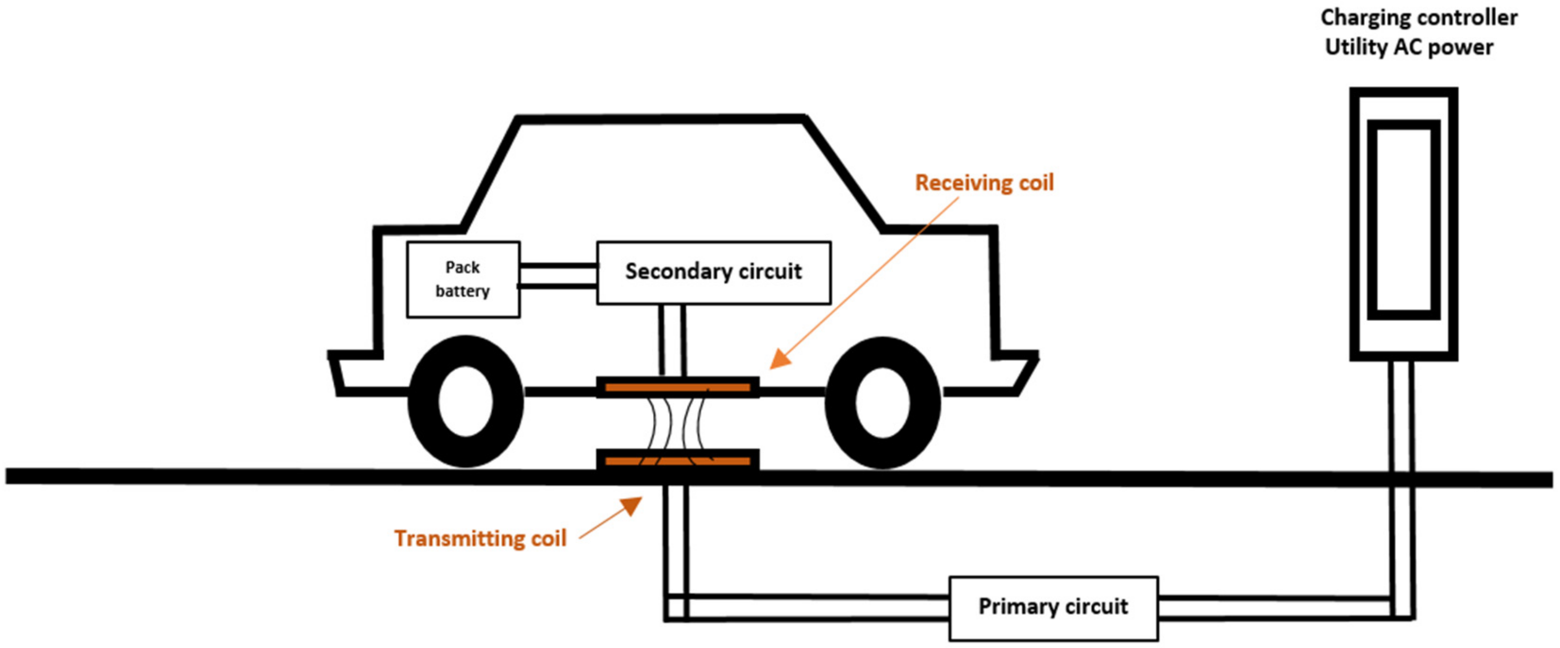
Figure 1.
The concept of WPT charging for the electric vehicle.
Figure 1.
The concept of WPT charging for the electric vehicle.
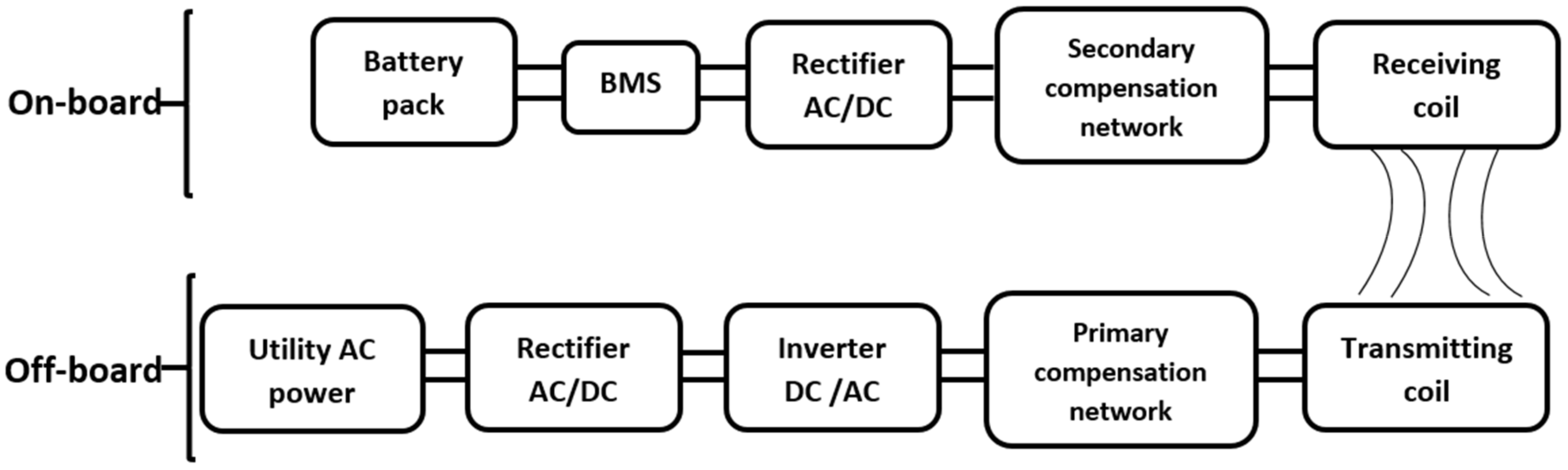
Figure 2.
Unidirectional magnetic resonance wireless power transfer for electric vehicle charging.
Figure 2.
Unidirectional magnetic resonance wireless power transfer for electric vehicle charging.
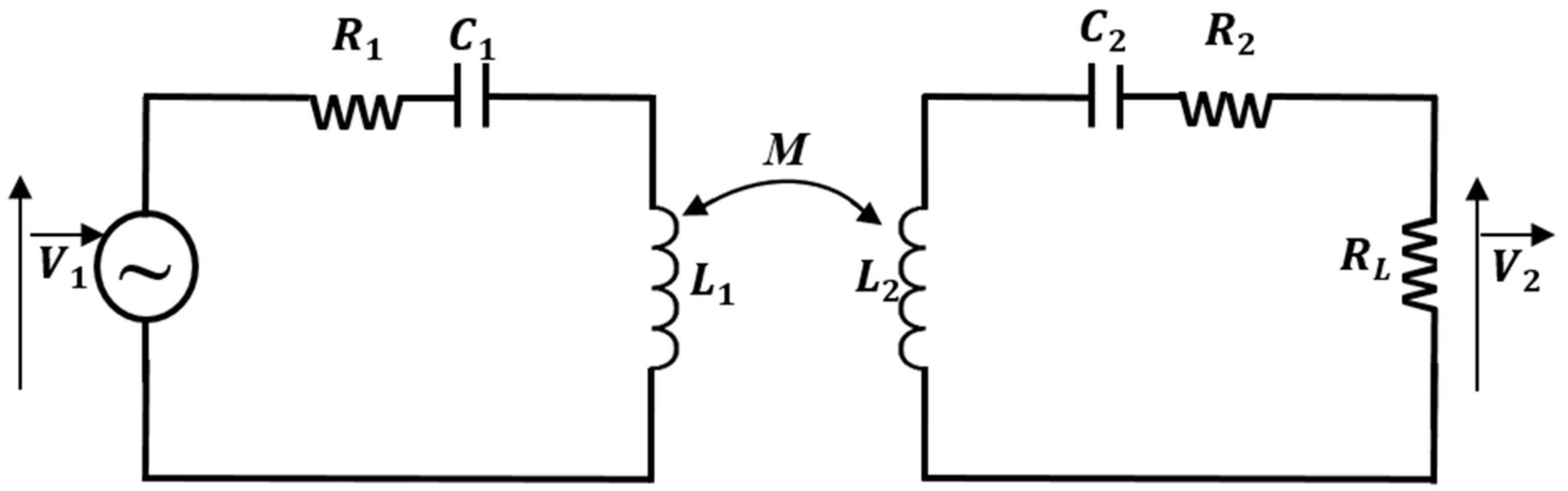
Figure 3.
Equivalent circuit of magnetic resonant WPT system.
Figure 3.
Equivalent circuit of magnetic resonant WPT system.
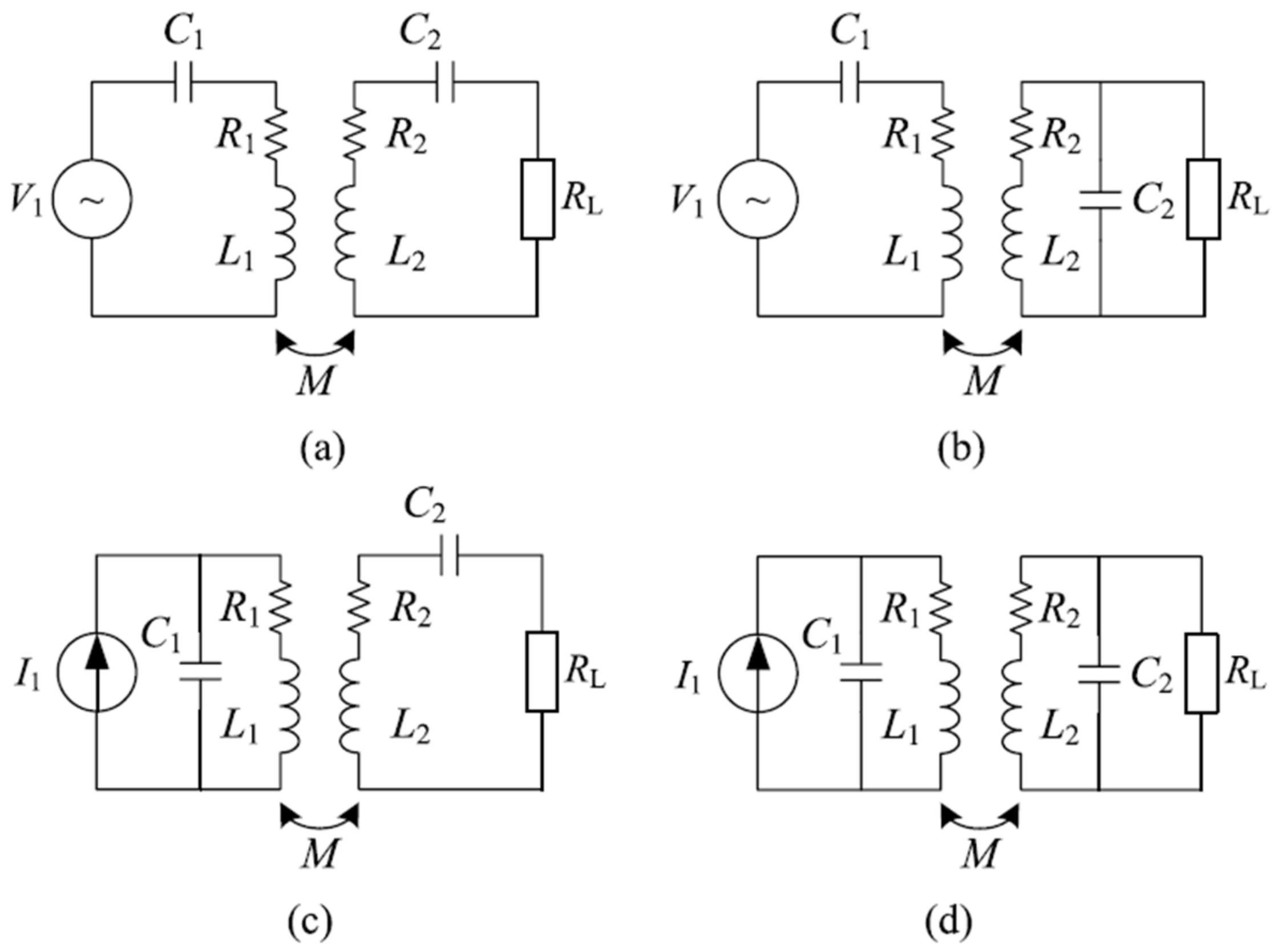
Figure 4.
Four basic compensation topologies. (
a) SS. (
b) SP. (
c) PS. (
d) PP [
22].
Figure 4.
Four basic compensation topologies. (
a) SS. (
b) SP. (
c) PS. (
d) PP [
22].
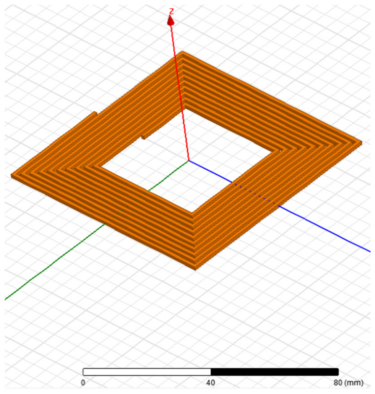
Figure 5.
Reference rectangular coil model.
Figure 5.
Reference rectangular coil model.
Figure 6.
Rectangular coil model for gap = 100 mm: (a) coreless model, (b) model with ferrite, (c) model with ferrite and aluminum.
Figure 6.
Rectangular coil model for gap = 100 mm: (a) coreless model, (b) model with ferrite, (c) model with ferrite and aluminum.
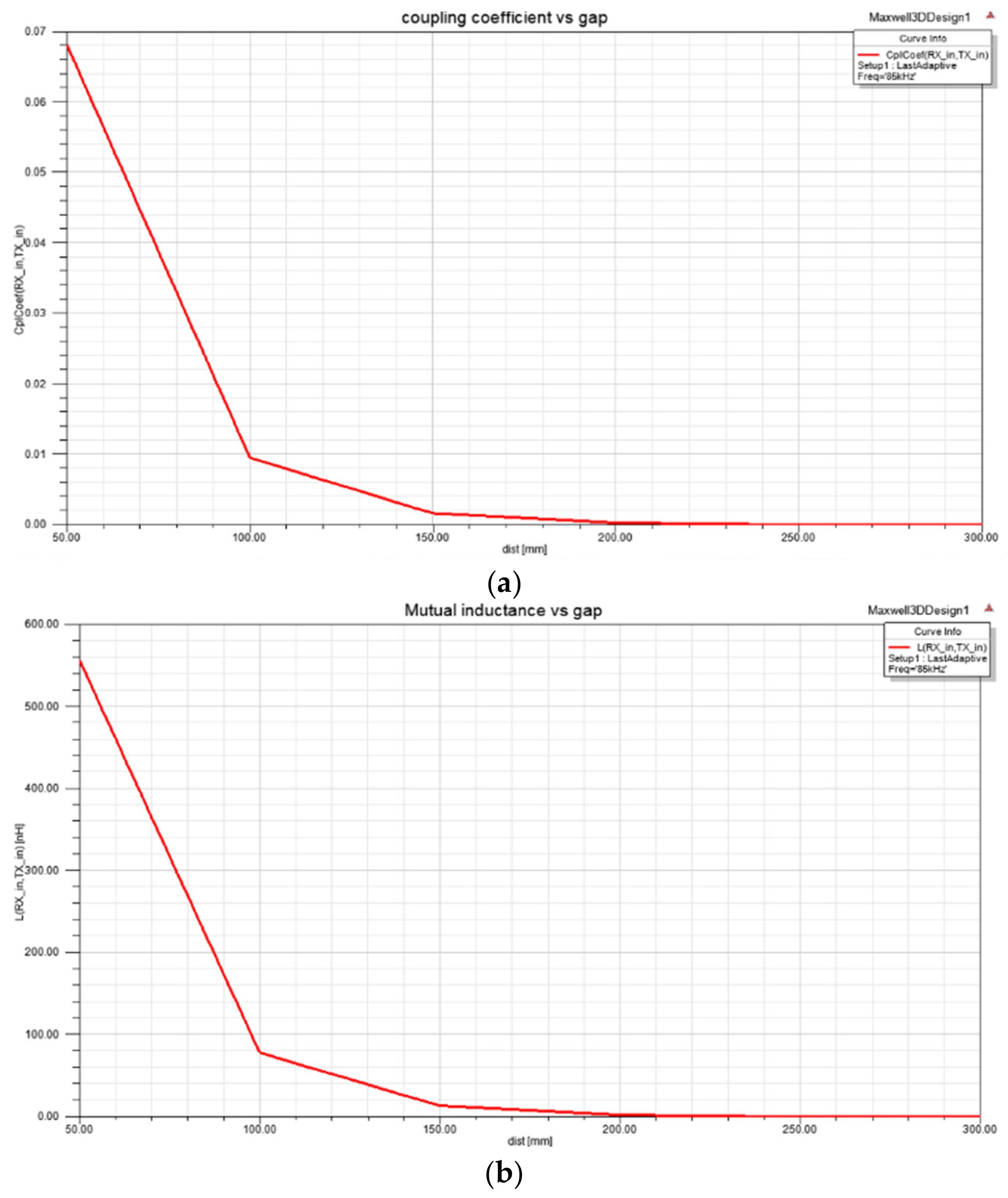
Figure 7.
Rectangular coreless model: (a) coupling coefficient versus the gap variation, (b) mutual inductance versus the gap variation.
Figure 7.
Rectangular coreless model: (a) coupling coefficient versus the gap variation, (b) mutual inductance versus the gap variation.
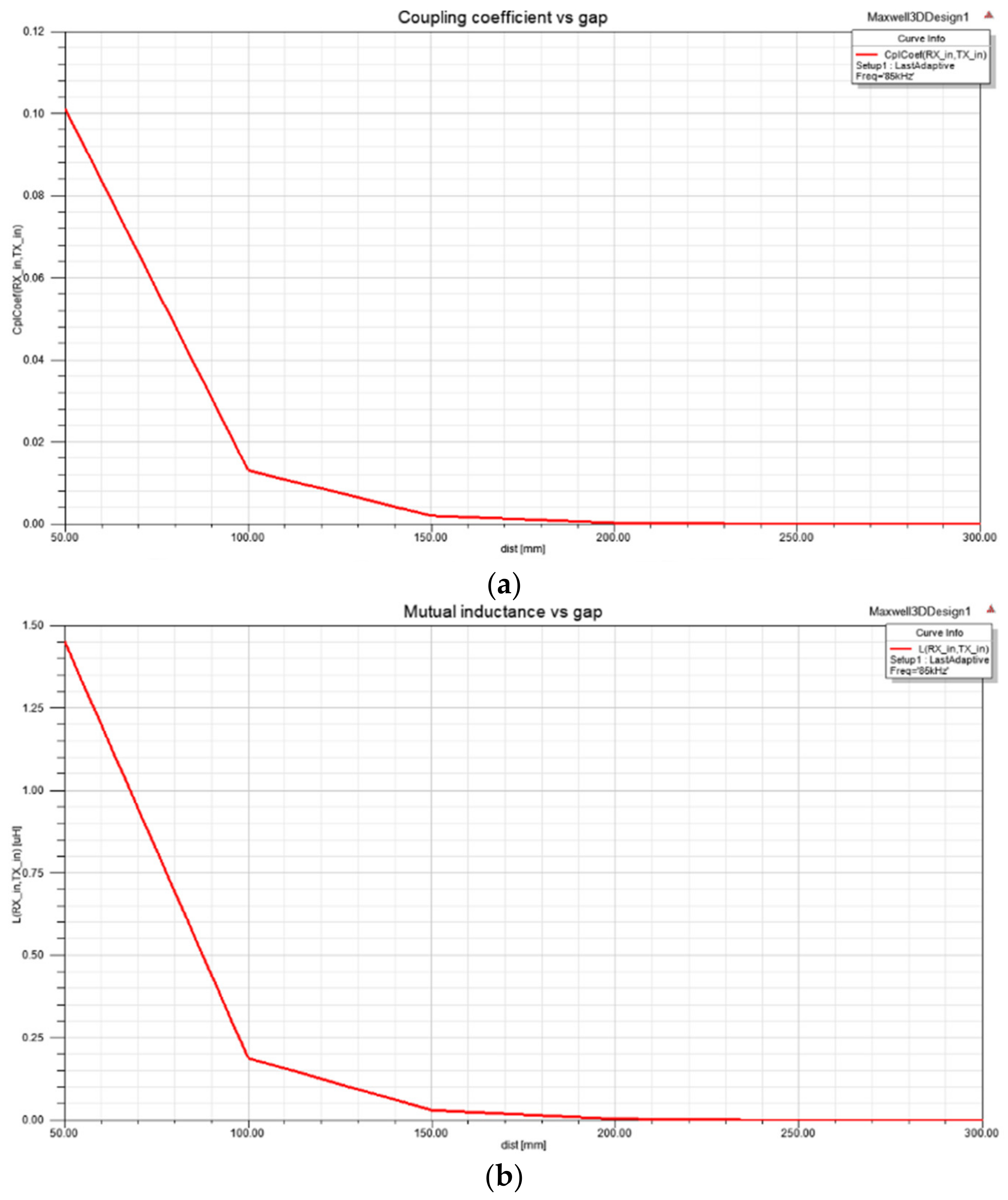
Figure 8.
Rectangular coil model with ferrite: (a) coupling coefficient versus the gap variation, (b) mutual inductance versus the gap variation.
Figure 8.
Rectangular coil model with ferrite: (a) coupling coefficient versus the gap variation, (b) mutual inductance versus the gap variation.
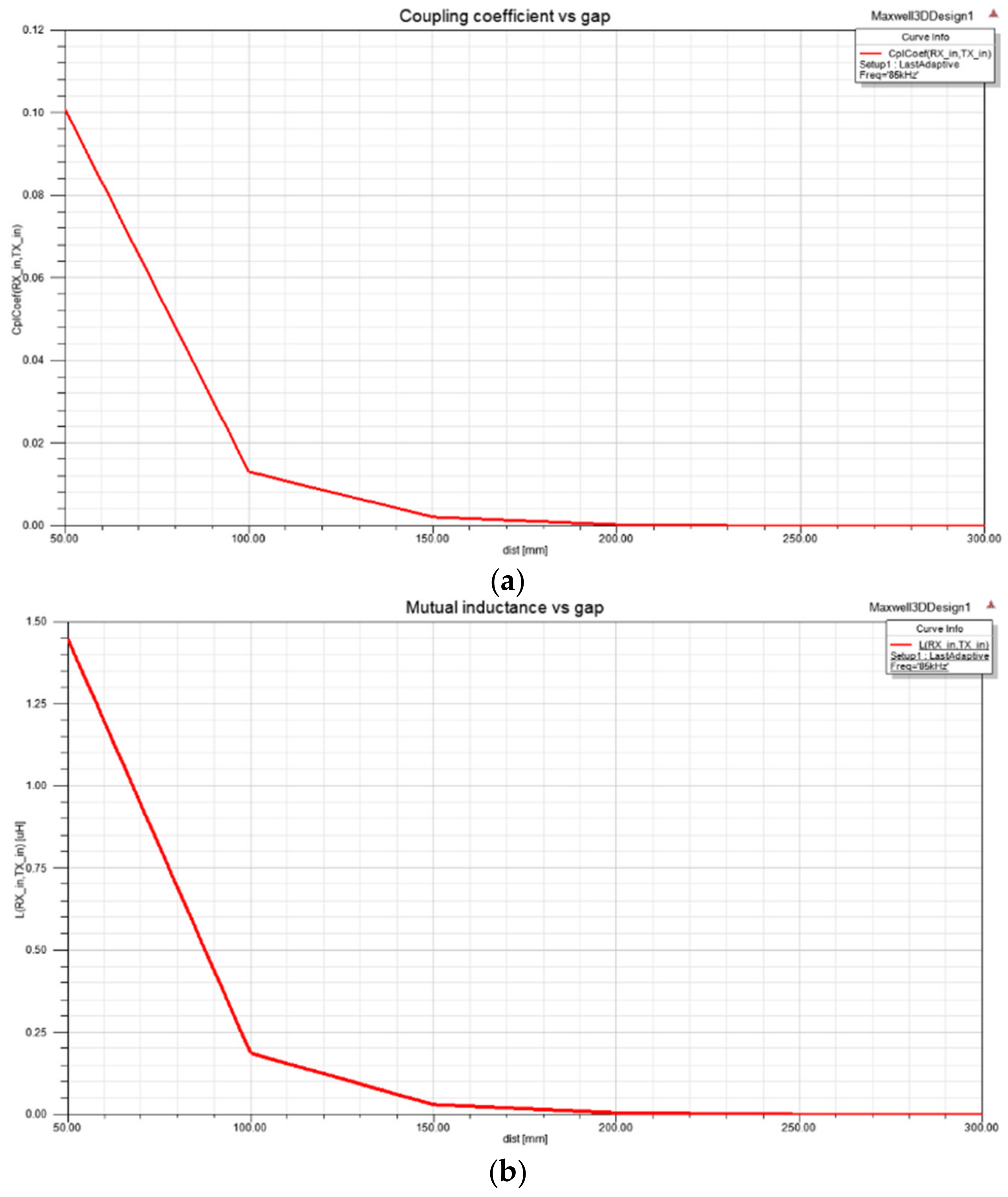
Figure 9.
Rectangular coil model with ferrite and aluminum: (a) coupling coefficient versus the gap variation, (b) mutual inductance versus the gap variation.
Figure 9.
Rectangular coil model with ferrite and aluminum: (a) coupling coefficient versus the gap variation, (b) mutual inductance versus the gap variation.
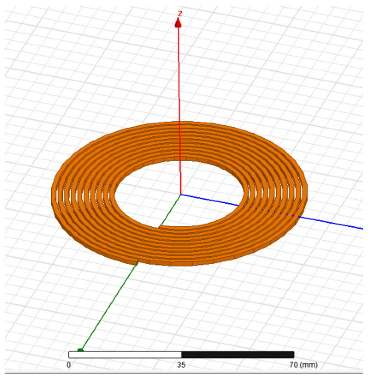
Figure 10.
Reference circular coil model.
Figure 10.
Reference circular coil model.
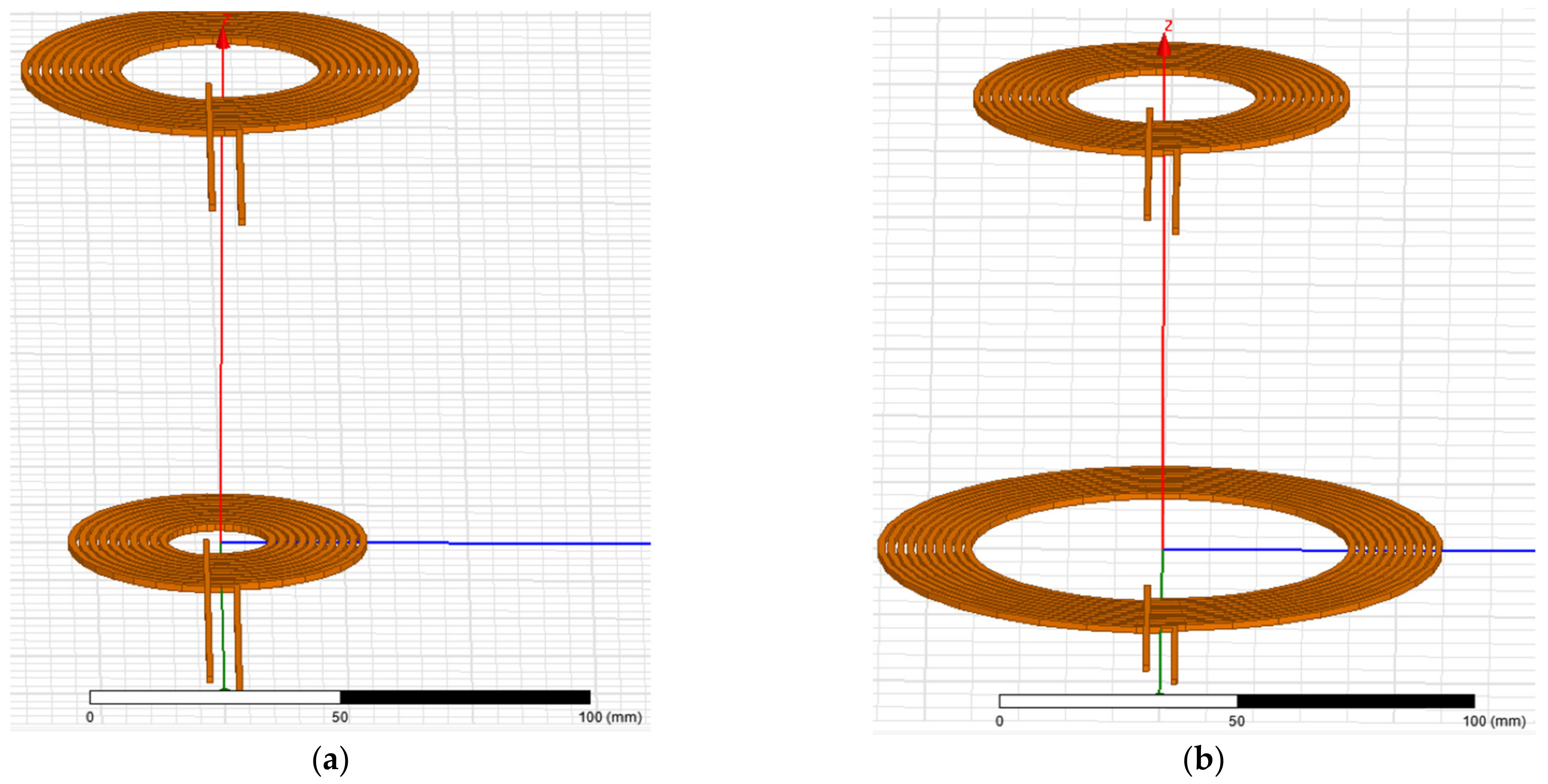
Figure 11.
Coreless coil models with constant : (a) mm, (b) mm for gap = 100 mm.
Figure 11.
Coreless coil models with constant : (a) mm, (b) mm for gap = 100 mm.
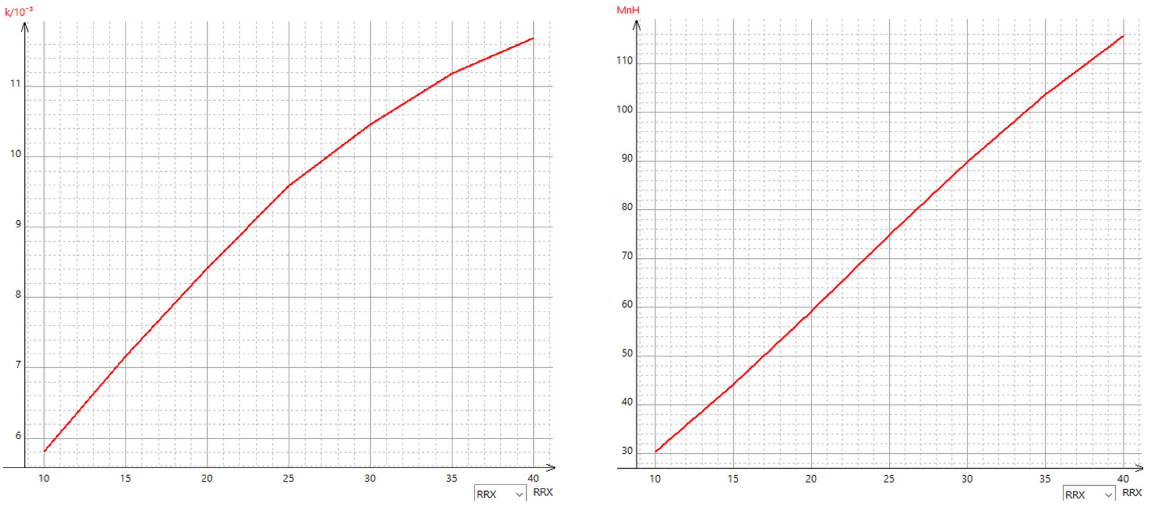
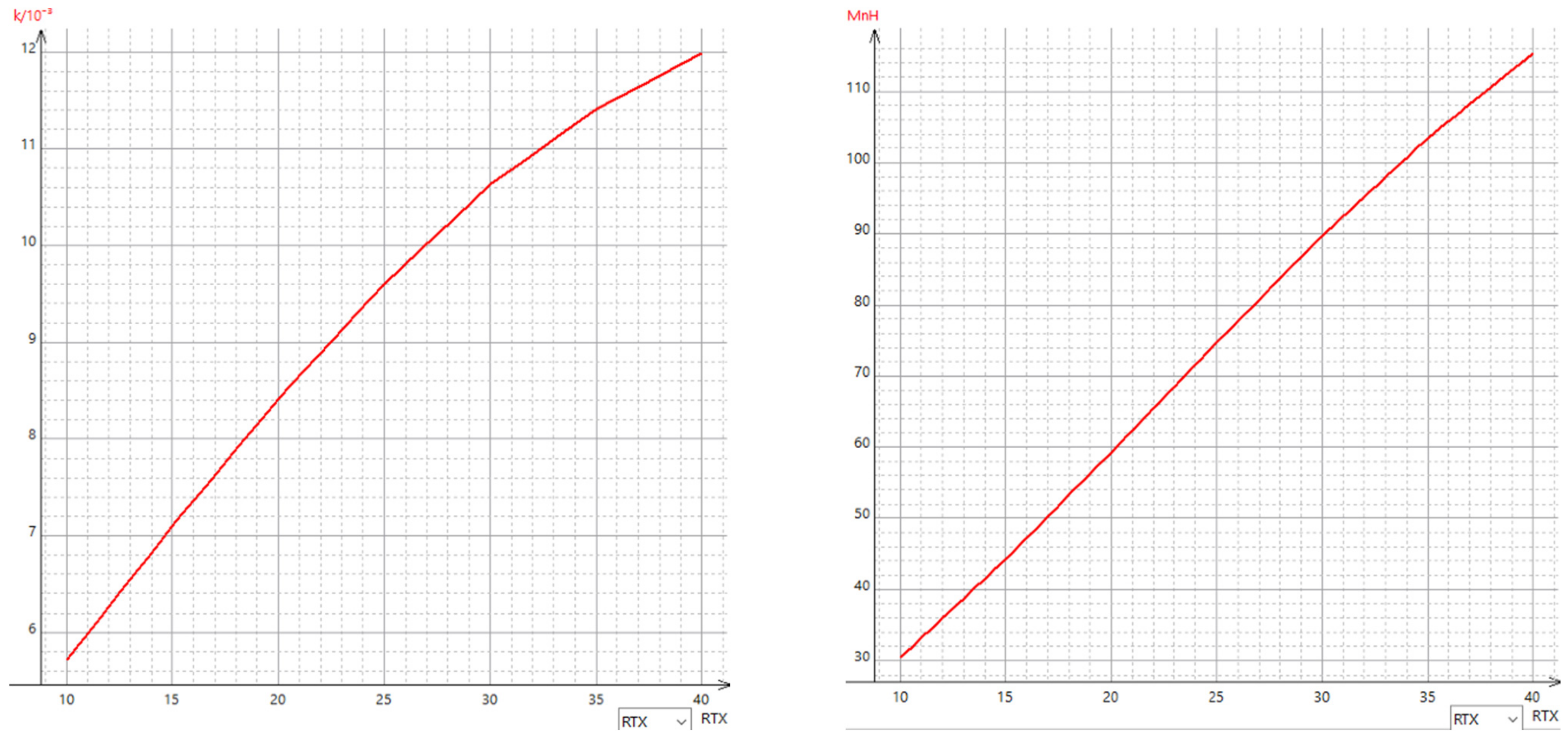
Figure 12.
variation simulation results of circular coil model: k in the function of and M in the function of .
Figure 12.
variation simulation results of circular coil model: k in the function of and M in the function of .
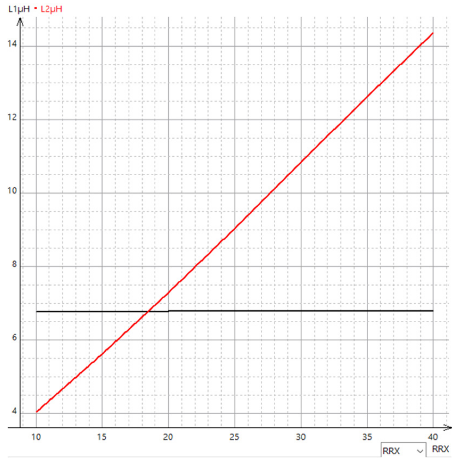
Figure 13.
variation simulation results of circular coil model: L1 in the function of , L2 in the function of .
Figure 13.
variation simulation results of circular coil model: L1 in the function of , L2 in the function of .
Figure 14.
Coreless coil models with constant : (a) mm, (b) mm for gap = 100 mm.
Figure 14.
Coreless coil models with constant : (a) mm, (b) mm for gap = 100 mm.
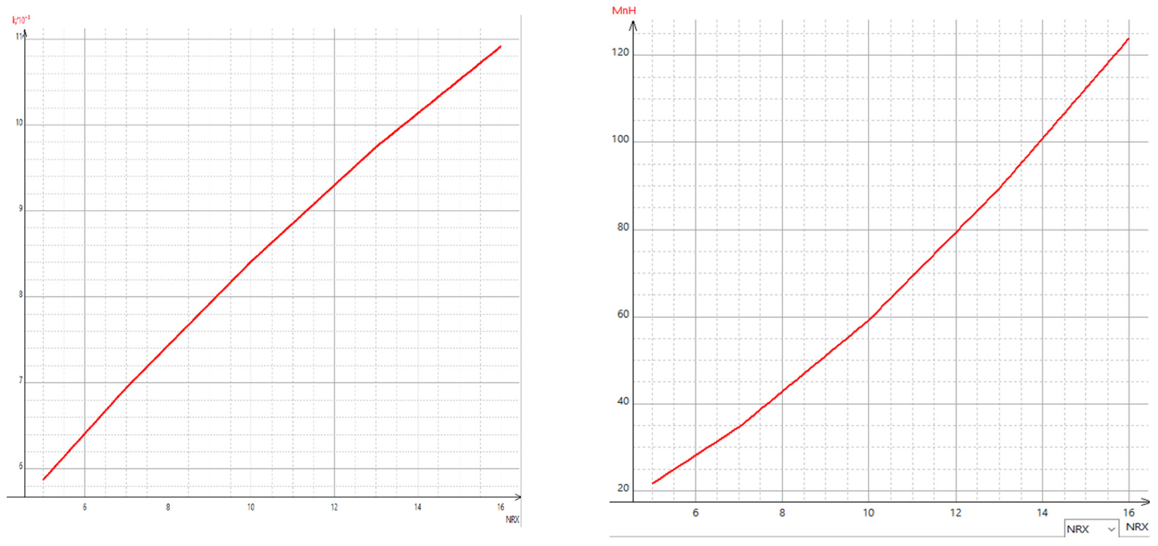
Figure 15.
variation simulation results of circular coil model: k in the function of , M in the function of .
Figure 15.
variation simulation results of circular coil model: k in the function of , M in the function of .
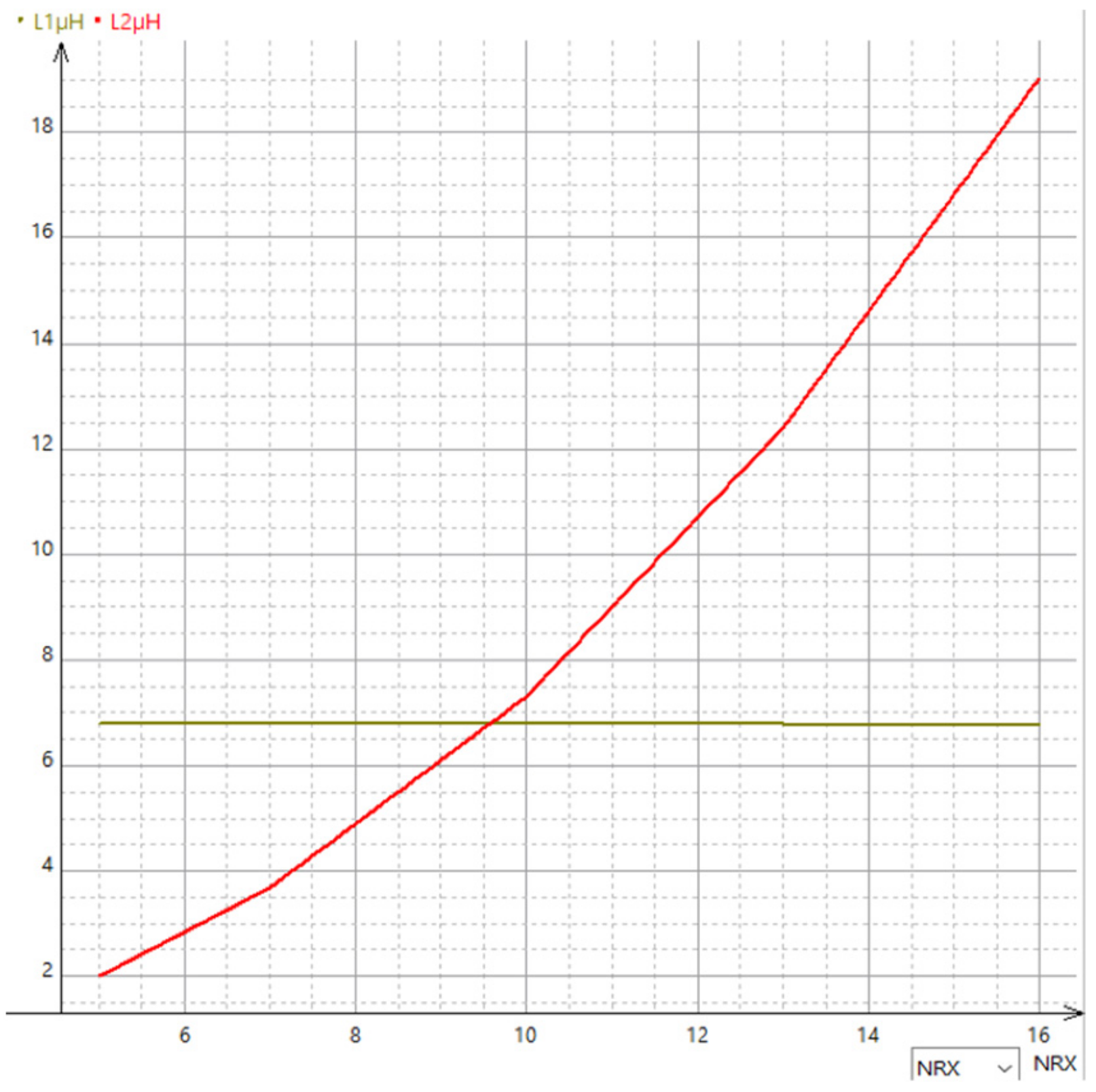
Figure 16.
variation simulation results of circular coil model: L1 in the function of , L2 in the function of .
Figure 16.
variation simulation results of circular coil model: L1 in the function of , L2 in the function of .
Figure 17.
A cross-sectional view of the flat circular coil.
Figure 17.
A cross-sectional view of the flat circular coil.
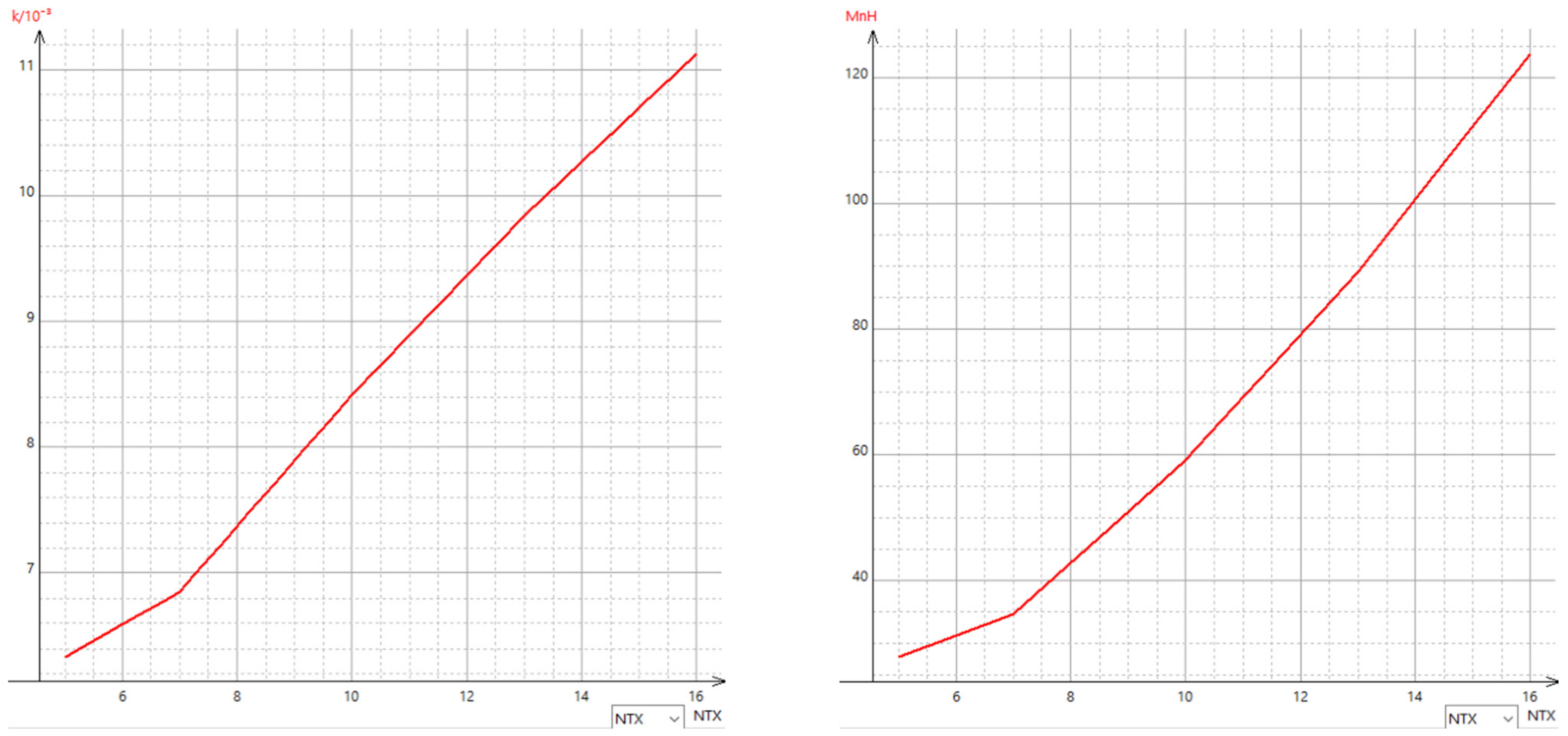
Figure 18.
Number of turns simulation results of circular coil model: k in the function of , M in the function of .
Figure 18.
Number of turns simulation results of circular coil model: k in the function of , M in the function of .
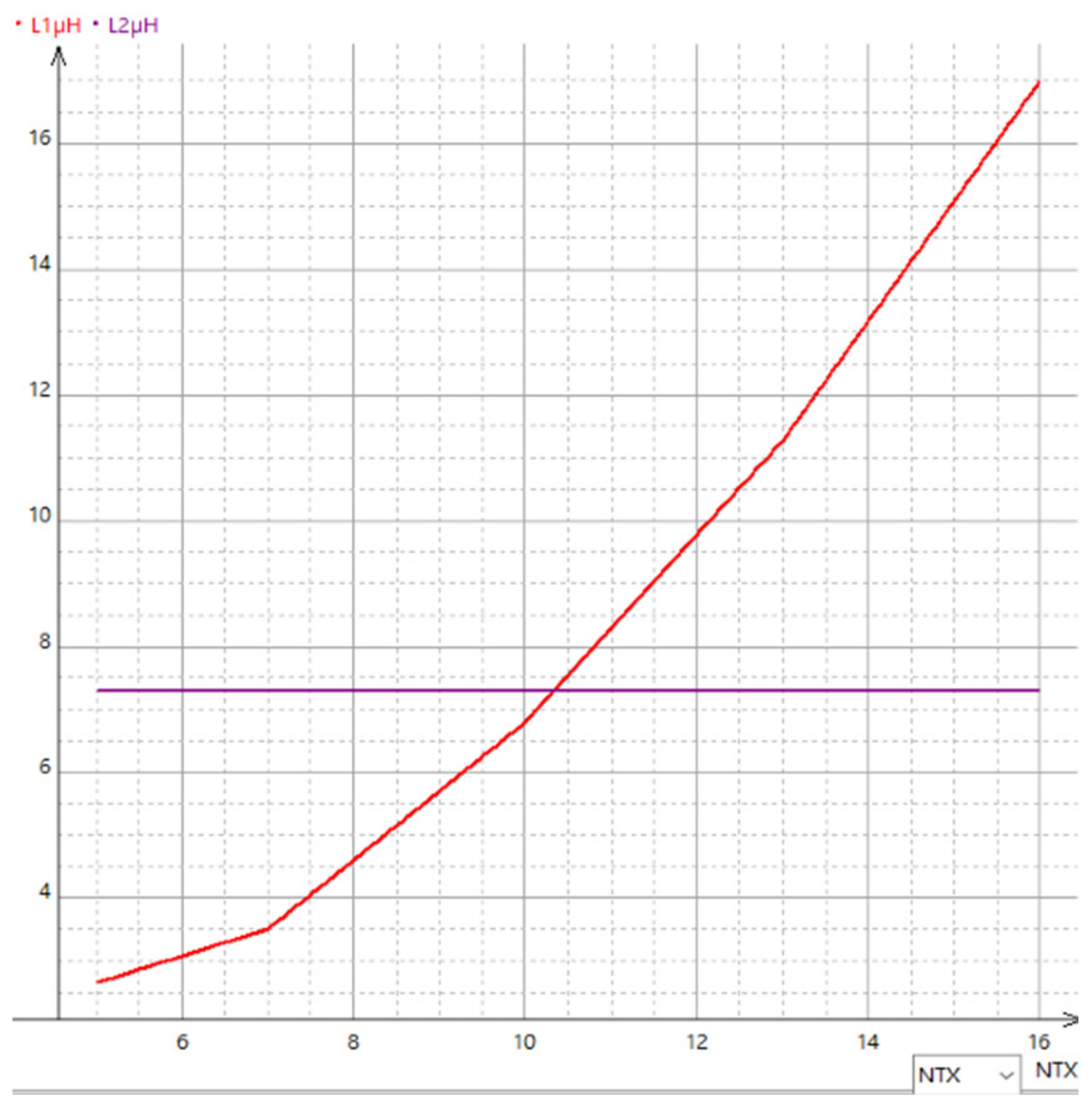
Figure 19.
Number of turns simulation results of circular coil model: L1 in the function of , L2 in the function of .
Figure 19.
Number of turns simulation results of circular coil model: L1 in the function of , L2 in the function of .
Figure 20.
Number of turns simulation results of circular coil model: k in the function of , M in the function of .
Figure 20.
Number of turns simulation results of circular coil model: k in the function of , M in the function of .
Figure 21.
Number of turns simulation results of circular coil model: L1 in the function of , L2 in the function of .
Figure 21.
Number of turns simulation results of circular coil model: L1 in the function of , L2 in the function of .
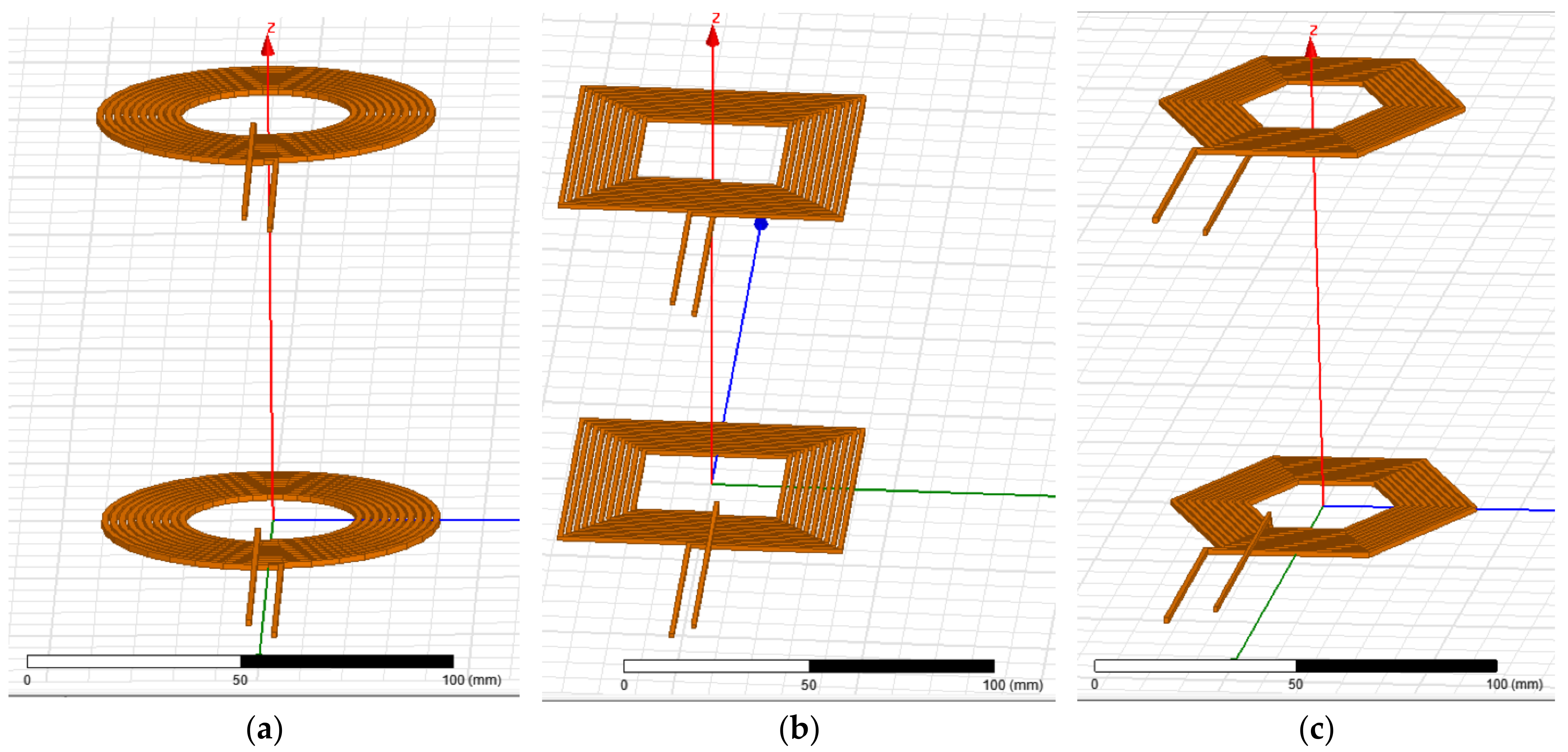
Figure 22.
The three cases: (a) circular coreless model, (b) rectangular coreless model, (c) hexagonal coreless model.
Figure 22.
The three cases: (a) circular coreless model, (b) rectangular coreless model, (c) hexagonal coreless model.
Table 1.
Default parameters for the model.
Table 1.
Default parameters for the model.
| Coil Material | Polygon Segment | Polygon Radius | Start Helix Radius | Radius Change | Winding Number of Turns | Segment per Turn | Pitch |
|---|
| copper | 4 | 1 mm | 20 mm | 2.05 mm | 10 | 36 | 0 |
Table 2.
Simulation results of rectangular coreless coil model.
Table 2.
Simulation results of rectangular coreless coil model.
| Gap (mm) | Coupling Coefficient | Mutual Inductance (nH) |
|---|
| 50 | 0.068109 | 556.24340 |
| 100 | 0.009552 | 78.193680 |
| 150 | 0.001664 | 13.567360 |
| 200 | 0.000319 | 2.609366 |
| 250 | 0.000054 | 0.427079 |
| 300 | 0.000000 | 0.000000 |
Table 3.
Simulation results of rectangular coil model with ferrite.
Table 3.
Simulation results of rectangular coil model with ferrite.
| Gap (mm) | Coupling Coefficient | Mutual Inductance (µH) |
|---|
| 50 | 0.101212 | 1.452432 |
| 100 | 0.013244 | 0.189907 |
| 150 | 0.002227 | 0.031972 |
| 200 | 0.000425 | 0.006089 |
| 250 | 0.000081 | 0.001156 |
| 300 | 0.000012 | 0.000169 |
Table 4.
Simulation results of rectangular coil model with ferrite and aluminum.
Table 4.
Simulation results of rectangular coil model with ferrite and aluminum.
| Gap (mm) | Coupling Coefficient | Mutual Inductance (µH) |
|---|
| 50 | 0.100854 | 1.448542 |
| 100 | 0.013164 | 0.188223 |
| 150 | 0.002217 | 0.031680 |
| 200 | 0.000423 | 0.006059 |
| 250 | 0.000081 | 0.001157 |
| 300 | 0.000013 | 0.000179 |
Table 5.
Circular coil model characteristics.
Table 5.
Circular coil model characteristics.
| Coil Material | Winding Number of Turns | Winding Diameter | Pitch |
|---|
| Copper | 10 | Outer 80 mm
Inner 40 mm | 0 |
Table 6.
Simulation results of circular coil model— variation.
Table 6.
Simulation results of circular coil model— variation.
| 10 | 15 | 20 | 25 | 30 | 35 | 40 |
|---|
| Coupling coefficient | 0.005816 | 0.007161 | 0.008412 | 0.009585 | 0.010463 | 0.011186 | 0.011684 |
| Mutual inductance (nH) | 30.424290 | 44.193950 | 59.199180 | 74.752330 | 89.813510 | 103.64980 | 115.51350 |
| L1 (µH) | 6.780342 | 6.779160 | 6.785520 | 6.791254 | 6.794025 | 6.793827 | 6.798295 |
| L2 (µH) | 4.036471 | 5.617566 | 7.298441 | 9.050857 | 10.844590 | 12.637880 | 14.37701 |
Table 7.
Simulation results of circular coil model— variation.
Table 7.
Simulation results of circular coil model— variation.
| 10 | 15 | 20 | 25 | 30 | 35 | 40 |
|---|
| Coupling coefficient | 0.005711 | 0.007095 | 0.008412 | 0.009605 | 0.010627 | 0.011418 | 0.011990 |
| Mutual inductance (nH) | 30.39108 | 44.18762 | 59.19918 | 74.67751 | 89.77743 | 103.5061 | 115.4117 |
| L1 (µH) | 3.874879 | 5.307868 | 6.785520 | 8.276253 | 9.770129 | 11.25197 | 12.68043 |
| L2 (µH) | 7.308522 | 7.308452 | 7.298441 | 7.303525 | 7.305497 | 7.302940 | 7.307154 |
Table 8.
Simulation results of circular coil model—number of turns variation.
Table 8.
Simulation results of circular coil model—number of turns variation.
| Number of Turns | 5 | 7 | 10 | 13 | 16 |
|---|
| Coupling coefficient | 0.005873 | 0.006941 | 0.008412 | 0.009744 | 0.010916 |
| Mutual inductance (nH) | 21.589390 | 34.704880 | 59.199180 | 89.343810 | 123.96730 |
| L1 (µH) | 6.784625 | 6.792092 | 6.785520 | 6.787126 | 6.774364 |
| L2 (µH) | 1.991499 | 3.680638 | 7.298441 | 12.386530 | 19.039200 |
Table 9.
Simulation results of circular coil model—number of turns variation.
Table 9.
Simulation results of circular coil model—number of turns variation.
| Number of Turns | 5 | 7 | 10 | 13 | 16 |
|---|
| Coupling coefficient | 0.006331 | 0.006856 | 0.008412 | 0.009836 | 0.011129 |
| Mutual inductance (nH) | 27.788710 | 34.660960 | 59.199180 | 89.228940 | 123.91930 |
| L1 (µH) | 2.639758 | 3.498766 | 6.785520 | 11.276280 | 16.990020 |
| L2 (µH) | 7.299475 | 7.304379 | 7.298441 | 7.298372 | 7.296844 |
Table 10.
The three coil main parameters.
Table 10.
The three coil main parameters.
| Inner Diameter | Outer Diameter | Number of Turns | Pitch | The Spacing between Adjacent Wires | Frequency | Initial Current |
|---|
| 40 mm | 80 mm | 10 | 0 | 0.7 mm | 85 kHz | 25 A |
Table 11.
The simulation results (k, M) of the three geometries: case 1, case 2, and case 3.
Table 11.
The simulation results (k, M) of the three geometries: case 1, case 2, and case 3.
| Gap (mm) | | | | | | |
|---|
| Case 1 |
| 50 | 0.063451 | 445.95400 | 0.068109 | 556.24340 | 0.057182 | 397.82520 |
| 100 | 0.008412 | 59.199180 | 0.009552 | 78.193680 | 0.007409 | 51.661350 |
| 150 | 0.001441 | 10.143700 | 0.001664 | 13.567360 | 0.001265 | 8.812501 |
| 200 | 0.000280 | 1.969708 | 0.000319 | 2.609366 | 0.000246 | 1.712719 |
| 250 | 0.000049 | 0.331442 | 0.000054 | 0.427079 | 0.000043 | 0.290551 |
| 300 | 0.000004 | 0.017259 | 0.000000 | 0.000000 | 0.000003 | 0.001513 |
| Case 2 |
| 50 | 0.087542 | 1.052032 | 0.101212 | 1.452432 | 0.086132 | 1.084909 |
| 100 | 0.010632 | 0.127913 | 0.013244 | 0.189907 | 0.010165 | 0.127640 |
| 150 | 0.001755 | 0.021099 | 0.002227 | 0.031972 | 0.001658 | 0.020777 |
| 200 | 0.000339 | 0.004080 | 0.000425 | 0.006089 | 0.000312 | 0.003920 |
| 250 | 0.000068 | 0.000811 | 0.000081 | 0.001156 | 0.000059 | 0.000740 |
| 300 | 0.000011 | 0.000125 | 0.000012 | 0.000169 | 0.000009 | 0.000103 |
| Case 3 |
| 50 | 0.064083 | 690.79670 | 0.100854 | 1.448542 | 0.085573 | 1.072621 |
| 100 | 0.006945 | 75.680240 | 0.013164 | 0.188223 | 0.010104 | 0.126605 |
| 150 | 0.001097 | 11.840260 | 0.002217 | 0.031680 | 0.001645 | 0.020617 |
| 200 | 0.000211 | 2.298739 | 0.000423 | 0.006059 | 0.000310 | 0.003883 |
| 250 | 0.000045 | 0.480430 | 0.000081 | 0.001157 | 0.000059 | 0.000734 |
| 300 | 0.000010 | 0.105318 | 0.000013 | 0.000179 | 0.000009 | 0.000110 |
Table 12.
The simulation results (, ) of the three geometries: case 1, case 2, and case 3.
Table 12.
The simulation results (, ) of the three geometries: case 1, case 2, and case 3.
| Gap (mm) | | | | | | |
|---|
| Case 1 |
| 50 | 0.064083 | 690.79670 | 0.100854 | 1.448542 | 0.085573 | 1.072621 |
| 100 | 0.006945 | 75.680240 | 0.013164 | 0.188223 | 0.010104 | 0.126605 |
| 150 | 0.001097 | 11.840260 | 0.002217 | 0.031680 | 0.001645 | 0.020617 |
| 200 | 0.000211 | 2.298739 | 0.000423 | 0.006059 | 0.000310 | 0.003883 |
| 250 | 0.000045 | 0.480430 | 0.000081 | 0.001157 | 0.000059 | 0.000734 |
| 300 | 0.000010 | 0.105318 | 0.000013 | 0.000179 | 0.000009 | 0.000110 |
| Case 2 |
| 50 | 11.947130 | 12.088330 | 14.298380 | 14.402650 | 12.562350 | 12.629550 |
| 100 | 11.950400 | 12.110930 | 14.266830 | 14.412460 | 12.513560 | 12.600940 |
| 150 | 11.957580 | 12.091200 | 14.256900 | 14.457540 | 12.474230 | 12.589890 |
| 200 | 11.926060 | 12.117880 | 14.263890 | 14.402940 | 12.515170 | 12.633200 |
| 250 | 11.941690 | 11.923480 | 14.226600 | 14.216720 | 12.504320 | 12.497870 |
| 300 | 11.808270 | 10.570560 | 14.300310 | 12.999270 | 12.510930 | 11.797060 |
| Case 3 |
| 50 | 10.781420 | 10.777930 | 14.281620 | 14.444460 | 12.492290 | 12.577110 |
| 100 | 10.869160 | 10.925570 | 14.209700 | 14.387980 | 12.471550 | 12.590100 |
| 150 | 10.792140 | 10.799971 | 14.204850 | 14.378430 | 12.469870 | 12.593910 |
| 200 | 10.903430 | 10.917850 | 14.243580 | 14.429750 | 12.455440 | 12.570840 |
| 250 | 10.785930 | 10.783920 | 14.226220 | 14.227060 | 12.458240 | 12.445430 |
| 300 | 10.864260 | 10.687310 | 14.189000 | 13.187760 | 12.458490 | 11.860980 |
Table 13.
Coefficients for current sheet expression.
Table 13.
Coefficients for current sheet expression.
| Layout | | | | |
|---|
| Square | 1.27 | 2.07 | 0.18 | 0.13 |
| Hexagonal | 1.09 | 2.23 | 0.00 | 0.17 |
| Octagonal | 1.07 | 2.29 | 0.00 | 0.19 |
| Circle | 1.00 | 2.46 | 0.00 | 0.20 |
Table 14.
The simulation results of coupling coefficient and mutual inductance for the nine models.
Table 14.
The simulation results of coupling coefficient and mutual inductance for the nine models.
| Gap (mm) | | | | | | |
| 50 | 0.063451 | 445.95400 | 0.065329 | 495.42490 | 0.060109 | 419.31340 |
| 100 | 0.008412 | 59.199180 | 0.008936 | 68.025210 | 0.007896 | 55.203930 |
| 150 | 0.001441 | 10.143700 | 0.001542 | 11.754990 | 0.001348 | 9.431740 |
| 200 | 0.000280 | 1.969708 | 0.000301 | 2.284551 | 0.000261 | 1.825223 |
| 250 | 0.000049 | 0.331442 | 0.000052 | 0.383236 | 0.000046 | 0.307663 |
| 300 | 0.000004 | 0.017259 | 0.000000 | 0.000000 | 0.000002 | 0.001061 |
| Gap (mm) | | | | | | |
| 50 | 0.065505 | 495.41300 | 0.068109 | 556.24340 | 0.061977 | 466.09330 |
| 100 | 0.008969 | 67.930470 | 0.009552 | 78.193680 | 0.008407 | 63.302460 |
| 150 | 0.001549 | 11.742200 | 0.001664 | 13.567360 | 0.001436 | 10.815340 |
| 200 | 0.000300 | 2.273186 | 0.000319 | 2.609366 | 0.000274 | 2.056993 |
| 250 | 0.000052 | 0.383192 | 0.000054 | 0.427079 | 0.000046 | 0.336436 |
| 300 | 0.000000 | 0.000683 | 0.000000 | 0.000000 | 0.000007 | 0.004216 |
| Gap (mm) | | | | | | |
| 50 | 0.059890 | 419.45510 | 0.061691 | 466.33140 | 0.057182 | 397.82520 |
| 100 | 0.007873 | 55.215220 | 0.008418 | 63.560160 | 0.007409 | 51.661350 |
| 150 | 0.001344 | 9.433949 | 0.001449 | 10.999020 | 0.001265 | 8.812501 |
| 200 | 0.000261 | 1.829159 | 0.000283 | 2.135191 | 0.000246 | 1.712719 |
| 250 | 0.000045 | 0.306498 | 0.000050 | 0.361493 | 0.000043 | 0.290551 |
| 300 | 0.000001 | 0.000207 | 0.000002 | 0.001336 | 0.000003 | 0.001513 |
Table 15.
The simulation results of transmitting and receiving coil inductance for the nine models.
Table 15.
The simulation results of transmitting and receiving coil inductance for the nine models.
| Gap (mm) | | | | | | |
| 50 | 6.781647 | 7.284003 | 6.784100 | 8.477065 | 6.785677 | 7.171434 |
| 100 | 6.785520 | 7.298441 | 6.808041 | 8.512145 | 6.801473 | 7.186742 |
| 150 | 6.785848 | 7.303122 | 6.812742 | 8.525414 | 6.804330 | 7.192457 |
| 200 | 6.785000 | 7.293397 | 6.801984 | 8.493260 | 6.789216 | 7.182279 |
| 250 | 6.781005 | 6.781653 | 6.794038 | 7.847548 | 6.786111 | 6.732637 |
| 300 | 6.773379 | 2.663993 | 6.768822 | 0.000010 | 6.769274 | 0.054358 |
| Gap (mm) | | | | | | |
| 50 | 7.840692 | 7.295153 | 7.859934 | 8.485935 | 7.861151 | 7.194426 |
| 100 | 7.844392 | 7.312895 | 7.852931 | 8.533822 | 7.871329 | 7.203291 |
| 150 | 7.857680 | 7.312504 | 7.833186 | 8.488914 | 7.867516 | 7.205843 |
| 200 | 7.859005 | 7.295325 | 7.866308 | 8.498958 | 7.859830 | 7.179874 |
| 250 | 7.853460 | 6.789841 | 7.866581 | 7.867194 | 7.859914 | 6.735969 |
| 300 | 7.833505 | 0.015037 | 7.844216 | 0.000008 | 7.843801 | 0.052946 |
| Gap (mm) | | | | | | |
| 50 | 6.720312 | 7.299205 | 6.733408 | 8.486042 | 6.739215 | 7.182131 |
| 100 | 6.727379 | 7.311488 | 6.714745 | 8.489664 | 6.753153 | 7.200412 |
| 150 | 6.728282 | 7.317937 | 6.751840 | 8.532690 | 6.738836 | 7.202593 |
| 200 | 6.730501 | 7.319607 | 6.717073 | 8.472698 | 6.734780 | 7.186359 |
| 250 | 6.718816 | 6.790786 | 6.761878 | 7.865598 | 6.749549 | 6.735351 |
| 300 | 6.709978 | 0.015512 | 6.707614 | 0.050624 | 6.705435 | 0.052990 |


