Influence of User Preferences on the Revealed Utility Factor of Plug-In Hybrid Electric Vehicles ^†

Abstract

Plug-in hybrid electric vehicles (PHEVs) are an effective intermediate vehicle technology option in the long-term transition pathway towards light-duty vehicle electrification. Their net environmental impact is evaluated using the performance metric Utility Factor (UF), which quantifies the fraction of vehicle miles traveled (VMT) on electricity. There are concerns about the gap between Environmental Protection Agency (EPA) sticker label and real-world UF due to the inability of test cycles to represent actual driving conditions and assumptions about their driving and charging differing from their actual usage patterns. Using multi-year longitudinal data from 153 PHEVs (11–53 miles all-electric range) in California, this paper systematically evaluates how observed driving and charging, energy consumption, and UF differs from sticker label expectations. Principal Components Analysis and regression model results indicated that UF of short-range PHEVs (less than 20-mile range) was lower than label expectations mainly due to higher annual VMT and high-speed driving. Long-distance travel and high-speed driving were the major reasons for the lower UF of longer-range PHEVs (at least 35-mile range) compared to label values. Enhancing charging infrastructure access at both home and away locations, and increasing the frequency of home charging, improves the UF of short-range and longer-range PHEVs respectively.

1. Introduction

Climate change, air quality, and public health concerns have necessitated that governments across the world implement policies to promote battery electric (BEVs) and plug-in hybrid electric vehicles (PHEVs), collectively addressed as plug-in electric vehicles (PEVs). In the U.S., the transportation sector is responsible for 30% of total national greenhouse gas (GHG) emissions, and the light duty vehicle (LDV) segment alone contributed close to 60% of total transport GHGs in 2017 [1]. In the state of California, 40% of total GHGs comes from the transportation sector, and the contribution from the LDV segment was close to 70% of transport GHGs [2]. California and many other governments have implemented a suite of technology forcing mandates, performance standards for transportation fuels, GHG emissions, and incentive-based policies to increase the market penetration of PEVs [3,4,5].

Plug-in hybrid electric vehicles are often considered to be a transitional technology with the potential to expedite the shift towards BEVs [6,7]. Plug-in hybrid electric vehicles are equipped with a larger battery pack compared to conventional hybrid vehicles (HEVs) that can be charged using grid electricity, and have an internal combustion engine (ICE). PHEVs are not limited by the range anxiety and higher upfront purchase cost concerns associated with BEVs, and they combine the pure electric driving capabilities of a BEV with the fuel and energy efficiency enhancements due to engine downsizing, low or no engine idling, and regenerative braking capabilities of an HEV. This design and operational flexibility allow them to be driven in Charge Depleting (CD) or Charge Sustaining (CS) mode depending on the source of motive power. Charge depleting (CD) mode can further be categorized into CD-EV and CD-blended (CDB) modes. In the CD-EV mode of operation, the entire motive power is provided by the electric motor by discharging the energy stored in the battery and the engine is never turned on. This type of operation is often called all-electric mode or zero emission (ZE) mode because only electricity is consumed and there are no tail-pipe emissions. Depending on the powertrain configuration, road network topology, speed and acceleration characteristics, and driver behavior, the engine may turn on to partially assist the motor in meeting the total propulsion energy demand in the CD mode. This is called CDB mode of operation because both electricity and gasoline are consumed, and the motive power is provided by the electric motor and the ICE. The CD mode of operation continues until the battery is depleted, after which the PHEV is operated in the CS mode as a regular HEV with the ICE providing the entire propulsion energy demand and only gasoline is consumed. Driving in the CD mode could be entirely electric VMT (eVMT) or a combination of electricity and gasoline (gVMT) VMT, whereas CS mode comprises of only gVMT.

A critical aspect while assessing the real-world environmental performance of PHEVs depends on the eVMT in the CD mode, which has direct implications on the fuel economy and exhaust emissions. In this regard, the concept of Utility Factor (UF) of PHEVs has been developed, which represents the proportion of VMT travelled on electricity. The formal procedures and test conditions under which the UF and the Environmental Protection Agency (EPA) “sticker label fuel economy” are estimated, are outlined in Society of Automotive Engineers (SAE) J1711 [8] and SAE J2841 [9] respectively. Standardized dynamometer certification cycles [10,11] are recommended in SAE J1711 to estimate the all-electric range (AER) and per-mile energy consumption in the CD-EV (kWh/mile) mode and miles per gallon (MPG) in the CS mode. Strictly speaking, AER or the charge depleting range, is the total miles traveled by a fully charged PHEV in the CD-EV mode prior to the first engine start event. To ensure parity and representativeness across geographies and socio-demographics with varying travel needs, the per mile energy consumption is weighted against national driving statistics such as the National Household Travel Survey (NHTS) [12] in order to determine at an aggregate level how much of a vehicle’s driving can be accomplished on CD mode in SAE J2841. The SAE J2841 explicitly assumes that:

• the PHEV starts its travel day on a fully charged battery;
• PHEV is fully charged once per day on days driven at the end of travel day trip at home;
• effect of additional intra-day charging and vehicle not being charged at the end of last trip nullify each other;
• travel patterns and VMT by PHEVs are identical to the self-reported single-day trip diary information of mainstream ICE users in the 2001 NHTS.

Due to its simplistic and selective set of assumptions, the J2841 may not adequately reflect how PHEVs are driven and charged in real-world conditions. Using year-long longitudinal data collected via on-board data loggers from 153 PHEVs (11–53 miles AER) in California, this paper systematically examines the disparities between observed PHEV driving, charging behavior and generalized expectations about their usage patterns, and its implications on UF estimates encapsulated in existing PEV policies.

Prior studies that relied on cross-sectional travel survey data like the NHTS broadly focused on understanding the sensitivity of UF to different assumptions about travel patterns and charging behavior. In [13] alternatives to the J2841 UF is proposed using the 2009 NHTS instead of the 2001 NHTS and a mid-day opportunistic charging, typically at the workplace, is also considered. Their study reported that the proposed UF is higher than the J2841 UF, but only for PHEVs with AER less than 65 miles. While the J2841 UF is strictly a distance based metric, Ref. [14] proposes an energy based UF. Sensitivity of UF to different vehicle attributes such as age, class, annual VMT, and charging behavior depending on dwelling unit type is examined, and their analyses indicates that UF is largely insensitive to vehicle class and dwelling unit type, but highly sensitive to annual VMT, age, and charging behavior [14]. With the availability of real-world driving data collected using loggers albeit from ICEs, efforts have been undertaken to develop a more realistic PHEV driving cycle compared to dynamometer cycles [10] in order to better estimate their real-world energy consumption and emissions [15]. The scope of such efforts expanded by incorporating additional charging opportunities based on dwelling times and location. High resolution GPS enabled travel data collected over a span of 18 months from 400 ICEs in the Seattle metropolitan area is utilized in [16] to investigate how UF would change if only home based tours are considered. Their study reports that gasoline and electricity prices have no statistically significant impact on the UF, and that workplace or away from home charging increases the UF only if the AER of PHEV is less than 40 miles. Studies also applied UF by utilizing longitudinal data from ICEs for evaluating the life-cycle costs, emissions, and value proposition of PHEVs [17,18], and optimal battery size design and its impact on market acceptance [19,20].

Around early 2011, a nationwide PEV demonstration and charging infrastructure deployment was undertaken as part of the EV project [21,22] to understand Chevrolet Volt and Nissan Leaf usage patterns across 20 different U.S. metropolitan regions. This was the first project at such a scale that offered insights into the performance PHEVs by directly observing their actual usage via telematics loggers. In [21] it is reported that the observed UF of approximately 800 Chevy Volts with 35 miles AER (2011–2012 model years) and 600 Chevy Volts (2013 model year) with 38 miles AER was higher than their respective SAE J2841 UF counterparts by at least 6%. Fewer share of long-distance travel days compared to the 2001 NHTS and charging more than once per day were attributed to be the reasons for deviating from J2841 UF estimates. A study of close to 60,000 Chevy Volts (2011–2014 model years) reported that the observed Volts were able to travel 74% of their total miles in CD-EV mode alone [23]. Charging more than once per day by taking advantage of day time opportunities was identified to be the major reason for exceeding the J2841 UF and EPA sticker label fuel economy estimates similar to the findings of [21,22]. In [24] a real-world fuel economy and UF of five PHEV models with 11–38 miles of AER is analyzed and their analysis indicates that deviation from certification cycle fuel economy were reported to be anywhere between 2% to 100% depending on the AER.

Most of the literature on PHEV usage focused on energy, emissions, and value proposition mainly from the perspective of driving. Reliable access to charging infrastructure is also important factor, because apart from user preferences, it is the availability of charging infrastructure that determines charger utilization and the charging demand. Understanding when, where, how long PHEVs are charged, and what the anticipated charging demand is are important factors for charging infrastructure developers from cost recovery, charger accessibility, user’s willingness to pay for charging, and charger utilization perspectives [25]. Utility companies are particularly concerned about the additional demand imposed on the grid from charging, as it has the potential to create localized hot spots if not managed properly, necessitating network upgrade or expansion. This highlights the importance of deploying coordinated or smart charging strategies that incorporate not only the economics of charging but also user preferences for charging location, time of day, duration of charging, and charging power levels [26]. Of particular concern are the competing objectives between the charging infrastructure developer and the user. The charging infrastructure developer seeks to minimize the cost of charging, which includes the fixed installation costs as well as the varying operating cost of providing electricity at the outlet. The PHEV driver, on the other hand, would like to maximize the convenience of charging without having to wait for a long duration, while simultaneously accomplishing this task at the lowest possible cost [27].

In summary, apart from the J2841 assumptions, the nature of travel data (longitudinal or cross-sectional), duration of data-collection, mode of data acquisition (self-reported trip diaries, data loggers with or without GPS), type of vehicle(s) used for data collection, and the targeted population (mainstream ICE users, actual PHEV owners or potential PHEV buyers) will also have consequential impacts on the techno-economic, electrification, and environmental benefits of PHEVs. The significance of UF cannot be understated since it is the vital environmental performance metric on which many federal and state level policies such as Corporate Average Fuel Economy (CAFE) and Pavley GHG emission standards [3,28,29], zero emission vehicle(ZEV) credit allocation under the ZEV mandate [30,31], vehicle emissions and label fuel economy estimates [32,33], and California’s Low Carbon Fuel Standards (LCFS) [34] rely on.

The main contributions of this study are the following:

• Comparative assessment of observed PHEV driving and charging and EPA sticker label expectations and the SAE J2841 assumptions.
• Eight dominant factors (four each for driving and charging) that explains the variations in observed PHEV usage patterns are extracted using Principal Components Analysis (PCA).
• Ordinary Least Squares (OLS) regression models are formulated to test the explanatory power of the factors by including them as dependent variables and the independent variable is the difference between observed and expected UF.
• Relative importance of the extracted factors in terms of their contributions to the disparities between observed and expected UF is then quantified.
• Though dimensionality reduction using PCA and regression modeling are commonly used, their specific application in the context of real-world observational study of PHEVs and UF is a new approach that is carried out in this study.

This paper advances to the body of literature that focuses on improving our understanding of the real-world UF of PHEVs by discerning influential driving and charging traits that contributes to the deviations from sticker label UF. To the best of our knowledge, compared to existing studies which limit their scope of analysis to either aggregate or daily levels [16,21,22,24,35], this paper focuses on explaining why real-world performance deviates from label expectations by methodically examining disparities at varying time-scales (trip/charging sessions, daily, and annual); incorporates locational aspects of charging infrastructure access and utilization and how it impacts the UF; and explores if the key driving and charging factors that introduces deviations in real-world UF from their label values are the same irrespective of the AER. The outcomes of this study will offer a realistic assessment of the real-world electrification potential of PHEVs, challenges, and/or validates conventional wisdom on PHEV usage, and subsequently their energy consumption and emissions. Understanding the causes, magnitude, and direction of differences between assumptions about PHEV usage and their observed usage will help the broader scientific community in parametric updates, calibration, and validation efforts to strengthen the representativeness or correct for the lack thereof in vehicle choice modeling [36], powertrain simulation tools [37], integrated assessment studies [38], charging infrastructure planning [39], and emissions inventory [40]. We expect the paper help in formulating policies aimed to incentivize PHEVs based on road performance and also to inform automakers when exploring future vehicle design.

The assemblage of data analyzed in this paper consists of driving and charging data collected between June 2015–June 2018 from 153 PHEVs in California. Five PHEV models are examined in this study: Toyota Prius (11-mile AER), Ford CMax and Fusion Energi (20-mile AER), Chevrolet Volts (35/38 miles and 53 miles AER). The rest of the paper is organized as follows. Section 2 summarizes the aggregate driving and charging data and describes the quantitative methods used. Our analysis and results are detailed in Section 3. Comparative assessment of observed driving and charging behavior with sticker label expectations, followed by the PCA and OLS model results are presented in Section 3. We discuss our findings in Section 4 and conclude this paper in Section 5.

2. Data and Methods

The source of the data used in this paper is from the Advanced PEV Driving and Charging Behavior project, a multi-year study to monitor PEV usage in California [41,42]. Online survey was first administered to PEV owners randomly sampled from the California Clean Vehicle Rebate Project [43] and vehicle registration records. Sub-sample of respondents were selected and GPS enabled data loggers were installed in the on-board diagnostics (OBD) port and monitored for at least a year. The data loggers report more than two dozen variables related to driving, charging, performance, and comfort. The important vehicle usage parameters relevant to our analysis are: trip and charging session start and ending time stamps and locations; trip and charging session start and end state of charge (SOC); charger level, charging duration, and charged energy; trip distances, duration, and consumption (electricity and gasoline). Since the scope of this paper is on real-world performance, our analysis strictly focuses on the data from the loggers, and the respondent’s home location is the only relevant survey information that is included in our analysis. Five PHEV models with sticker label AER varying from 11–53 miles [44] are in the dataset: Toyota Prius (11 miles AER, N = 22), Ford CMax Energi (20 miles AER, N = 28), Ford Fusion Energi (20 miles AER, N = 24), Chevrolet Volts (35/38 miles AER, N = 43; 53 miles AER, N = 36). The 35- and 38-mile AER Chevy Volts were grouped together as Volt-35/38 since there was little difference between their AER capabilities. The PHEV models analyzed in this study accounted for close to 85% of rebates issued to PHEVs under the California Clean Vehicle Rebate Project [43].

2.1. Driving and Charging Data

Table 1. Aggregate driving and charging data.

				Distance in Miles		Charging (L1 and L2)		L1/L2 Share (%)
PHEV Model	N	Driving Days	Trips	VMT	eVMT	Sessions	Charged kWh	Sessions
Prius-11	22	6921	33,421	315,166	46,573	7677	17,618	92/8
Cmax-20	28	7516	33,434	322,526	122,732	9796	36,100	57/43
Fusion-20	24	6972	34,028	346,720	108,136	9615	34,528	48/52
Volt-35/38	43	12,574	53,274	557,498	355,048	15,292	96,046	47/53
Volt-53	36	10,663	47,475	414,803	281,372	9857	73,956	33/67
Total	153	44,646	201,632	1,956,713	913,862	52,237	258,248

presents the driving and charging data which consists of approximately 2 million VMT, 200,000 trips, 52,000 charging sessions, and 260 MWh of charging energy collected over the course of 45,000 driving days (driving and charging or driving only) between June 2015–June 2018 in California. On average, every vehicle in the dataset was driven 292 days, and among the PHEV types it varied between 268 and 315 days during the data collection period. Of the 52,237 charging sessions, 53% were at Level 1(L1), 1.4 kW rated and the rest were at Level 2 (L2), 3.3 kW rated [45]. Throughout the rest of the paper, unless otherwise specified, J2841 UF [9], AER and mode specific energy consumption, kWh/mile in CD-EV mode or Miles Per Gallon(MPG) in CS mode, found in EPA fuel economy labelling data [46] are collectively addressed as Expectations. The label UF refers to the EPA sticker label city/highway combined UF. Corresponding values estimated from the data analyzed in this study as Observed.

Table 2. Average annualized and daily driving and charging metrics.

	Annualized			Average daily
PHEV Model	eVMT	gVMT	VMT	Charging Sessions	Charged kWh	VMT
Prius-11	2456	14,165	16,621	1.12	2.6	45.5
Cmax-20	5960	9703	15,663	1.32	4.9	42.9
Fusion-20	5661	12,489	18,151	1.39	5.0	49.7
Volt-35/38	10,306	5877	16,183	1.23	7.8	44.3
Volt-53	9632	4567	14,199	0.95	7.1	38.9

presents the average annualized and daily estimates of key PHEV driving and charging metrics.

2.2. Quantitative Methods

Principal Component Analysis (PCA) is a statistical procedure to reduce the dimensionality of the dataset and it falls under the larger umbrella of Exploratory Factor Analysis (EFA). In this paper, we use PCA to reduce the dimensionality of the observed driving and charging data which is highly susceptible to the problem of multicollinearity. Since Utility Factor is the ratio of eVMT to VMT and eVMT is a function of charging behavior, multicollinearity would persist and as such could severely undermine interpreting the statistical significance of driving and/or charging related independent variables (IV) on the dependent variable (DV). Combining both driving and charging related usage metrics and then performing the PCA may not eradicate the problem of multicollinearity. A correlation that existed in the higher dimensional space of the original data merely gets transformed and projected onto a new and lower- dimension space. This could complicate factor definition, number of factors to retain, determining the minimum loading criteria, and the rotation method to choose. To address these issues, we performed PCA of driving and charging related variables separately.

2.2.1. Validity and Suitability of the Data for PCA

The EFA involves four major steps. The first step is to check the appropriateness of the dataset for factor analysis. For this, we used the Kaiser-Meyer-Olkin (KMO) Measure of Sampling Adequacy (MSA) [47,48] and Bartlett’s Test for Sphericity [49]. The KMO MSA is an index between 0–1 which quantifies the ratio of observed correlations to partial correlations, the higher the better indication of the suitability of PCA [50,51]. Literature recommends a empirical rule of thumb of at least 0.6 as a minimum for the KMO MSA [52,53]. Bartlett’s Test for Sphericity tests the hypotheses that the correlation matrix is an identify matrix, thereby implying that variables are unrelated and not suitable for PCA. Bartlett’s test with a p-value of less than 0.05 is required for PCA. The KMO and Bartlett’s tests together determine whether the underlying structure of the dataset is suitable before proceeding to perform the PCA. The second step is to decide how many factors to retain. The number of factors to extract and retain is typically determined based on the share of variance explained by each of the factors and a suitable threshold for the cumulative total variance captured by the PCA. Scree plot for Eigen Value of greater than one is a widely used method to select the number of factors to retain, which this paper employed. The resultant component matrix shows the factor loadings or correlation between variables used for PCA (row-wise) and the factors (column-wise). Factor loadings outside the interval of ±0.3 are typically omitted [53,54]. The third step is to rotate the component matrix to simplify their structure and facilitate their interpretation. There are two major categories of factor rotation, Orthogonal and Oblique [55]. In orthogonal rotation, the factors are rotated by 90° to make them un-correlated, whereas in Oblique rotation, correlation between extracted factors are permissible. Varimax and Quartimax are the commonly used orthogonal rotation methods. The Quartimax method minimizes the number of factors needed to explain each variable used in the PCA and the Varimax method of rotation causes each variable to load heavily on one factor [56,57,58]. We used the Varimax method because of the simplicity of interpretation. Since the factors themselves are not correlated, Varimax rotated factors can be used in assessing the explanatory power of the factors in a regression model. The fourth and final step is to suitably name the rotated factors based on the factor loadings.

The aggregate driving and charging data of 153 PHEVs was first annualized based on the number of days every PHEV was driven. Using PCA, we identified four dominant driving and charging factors, eight in total. In this paper, the KMO MSA was close to 0.8 for both the driving and charging related PCA, which is considered “meritorious” [47,50,51]. The p-value of Bartlett’s test was extremely low and lower than the significance level of 0.05 for both the driving and charging related PCA, the data is suitable for PCA. The extracted factors captured 87% of the total variance in the dataset. Variables used for PCA, extracted factors, and their definitions are detailed in Section 3.2.

2.2.2. OLS Model Development

To test the explanatory power of the extracted factors, we built Ordinary Least Squares (OLS) multi-variate linear regression models with the extracted factors as the independent variables (IVs), and the deviation of observed UF from label UF as the dependent variable (DVs). The dataset was divided into two based on the AER: short-range PHEVs (Prius, Ford CMax/Fusion Energi) and long-range PHEVs (Volts). OLS regressions models for short-range PHEVs and long-range PHEVs were developed separately. We carried out a-priori and post-hoc hypothesis tests and validated that the sample size and power are adequate for the given significance level (5%) and sample size for both models. To supplement the insights gathered from the regression models and gauge the practical utility rather than just their statistical significance of the IV, we performed a relative importance analysis of each of these extracted factors by quantifying their main and total effects. The main effect is the contribution by an IV to the total variance by itself, and the total effect is the contribution by an IV to the total variance in combination with other IVs [59,60,61]. We also examined the effect of including interaction terms in the regression models. The regression model estimates and outcomes of the relative importance analysis are detailed in Section 3.3. The PCA was done using IBM SPSS and the OLS regression modeling, and relative importance analysis were carried out using JMP Pro 15.3.

3. Analysis and Results

In this section, we compare real-world performance of observed PHEVs with sticker label expectations from the perspectives of UF, daily driving distances and style, mode specific energy consumption, and charging behavior. Wherever applicable, we also contrast driving and charging behavior observed among the five PHEV models studied in this paper.

3.1. Descriptive Comparisons

3.1.1. Observed UF and Expected UF

Figure 1 depicts the UF distribution of every PHEV observed in this study. The EPA label expected city/highway combined UF is shown inset in Figure 1 as well. Except for the Volt-35/38, all the other PHEV models performed below EPA expectations, and the deviations were most notable in the case of short-range PHEVs (AER 20 miles or less) compared to the longer-range PHEVs (35 miles or more AER). On average, the observed UF was anywhere between 60–103% of label UF. Figure 2 shows the ratio of observed UF to label UF and its distribution by PHEV type. The observed UF of 82% (N = 18) of the Prius, 75% (N = 18) of Fusion, 66% (N = 24) of Volt-53, 54% (N = 15) of CMax, and 44% of Volt-35/38 (N = 19) were lower than the label UF estimates. Two interesting observations can be gleaned from Figure 1 and Figure 2. First, the range of UF deviations is higher for shorter-range PHEVs (Prius, CMax, and Fusion) compared to longer-range PHEVs (Volts); secondly, there are few short-range PHEVs that rarely or never plug in and are operated as a regular HEV. Referring to Table 2, the annual VMT of PHEVs observed in this study is higher than estimates reported in other real-world PHEV usage studies [3,22,23,62]. From we can except for the Volt-35/38, the UF of PHEVs observed in this study (Figure 1 and Figure 2) was lower than the values reported in [3,22,23,62].

3.1.2. Observed Driving Styles and EPA Dynamometer Test Cycles

Figure 3a shows the percentage share of total driving time based on driving speed in mph of the observed PHEVs and Figure 3b depicts the share of total driving time by driving speed of certification cycles commonly used in fuel economy and exhaust emissions measurements. The Urban Dynamometer Driving Cycle (UDDS) and Highway Fuel Economy Testing (HWFET) represent urban/city driving cycle and highway driving conditions (under 60 mph) respectively [10,29,63]. The Federal Test Procedure (FTP) is an extension of the UDDS which consists of the UDDS, followed by the first 505 seconds of the UDDS. The US06 is a high speed and acceleration aggressive highway driving cycle used by the California Air Resources Board (CARB) to determine additional credit allocation under its ZEV mandate [64]. Driving style within the context of this study refers to attributes such as stop frequency per mile, percentage share of driving time, and distance driven at different speeds.

Figure 3 indicates some clear trends and divergences among the observed PHEVs, as well as between the observed PHEVs and test cycles. Volts (Volt-35/38 and Volt-53 combined) have a higher fraction of idling time and lower fraction of time in highway driving conditions (60 mph or more) compared to shorter-range PHEVs. We can observe a certain level of conservativeness in driving style by the Volt-53 if we compare their share of time at different speeds, which gradually decreases with an increase in speed. It can be noticed from Figure 3 that shows that the test cycles do not adequately capture how the driving style varies among PHEVs with different AER capabilities. Moreover, the test cycles either underestimate or completely exclude the share of driving at highway speeds (60 mph or more).

Figure 4 shows the distribution of stops per mile at a trip level. Figure 4a shows the cumulative distribution and Figure 4b shows the probability density function. For reference, stops per mile of HWFET, UDDS, and FTP is also indicated in Figure 4. It is interesting to note that the share of trips made with stop frequency lower than UDDS stop frequency per mile increases with AER, and varied from 60% for the Volt-53, to 75% for the Prius.

Figure 5a shows the percentage share of total distance driven at different speed intervals among the observed PHEVs and Figure 5b shows the percentage share of total distance driven at different speed intervals under EPA test cycles. Approximately 40% of total distance was driven at highway speeds (60 or more mph), and the shorter-range PHEVs had a slightly higher share of travel at 60 mph or more compared to the Volts. As found in Figure 3b, majority of the city/urban or highway test cycles overestimate the share of travel at 45 mph or less, especially UDDS in the case of travel at 15–30 mph. Figure 3, Figure 4 and Figure 5 clearly illustrate that the test cycles are more conservative when compared to the real-world driving style of PHEVs. The gap between observed driving and test cycles, especially highway speed driving, manifests in the form of deviations in the real-world fuel economy and UF.

Since high-speed driving consumes more energy (gasoline and/or electricity) compared to city or stop-and-go driving, the effective AER, fuel economy, and UF realized on-road by a fully charged PHEV could be lower than their respective sticker label estimates. This is highlighted in

Table 3. Comparison of label expected and observed ZE and CS mode energy consumption.

	CD-EV or ZE Mode Trips kWh/mile			CS Mode Trips MPG
	Label	Observed	$\left(\frac{\mathbf{O}\mathbf{b}\mathbf{s}\mathbf{e}\mathbf{r}\mathbf{v}\mathbf{e}\mathbf{d}}{\mathbf{L}\mathbf{a}\mathbf{b}\mathbf{e}\mathbf{l}}\right)$	Label	Observed	$\left(\frac{\mathbf{O}\mathbf{b}\mathbf{s}\mathbf{e}\mathbf{r}\mathbf{v}\mathbf{e}\mathbf{d}}{\mathbf{L}\mathbf{a}\mathbf{b}\mathbf{e}\mathbf{l}}\right)$
Prius-11	0.29	0.33	87.9%	50	48	96.0%
Cmax-20	0.37	0.39	94.9%	38	40	105.3%
Fusion-20	0.37	0.40	92.5%	38	40	105.3%
Volt-35/38	0.35	0.36	97.2%	37	34	91.9%
Volt-53	0.31	0.38	81.6%	42	38	90.5%

and Figure 6. Table 3 compares the label and observed CS mode fuel economy in miles per gallon (MPG) and CD-EV or ZE mode per mile electricity consumption (kWh/mile) and Figure 6 shows their respective distributions of the CS mode MPG and CD-EV mode kWh/mile observed. On average, the observed CS mode fuel economy and ZE mode electricity consumption per mile was lower than the sticker label values for the Prius and Volts (Volt35/38 and Volt-53). In the case of CMax and Fusion, their CS mode fuel economy was slightly higher than sticker label values but their CD-EV mode kWh/mile was lower than the label values. From Table 3, we can infer that the disparities between label and observed ZE mode kWh/mile translates into the effective AER realized on-road being 3–18% lower than of label AER. In the proceeding sub-sections, we specifically focus on driving and charging varied among the five PHEV models analyzed in this paper.

3.1.3. Daily VMT Comparisons among the Observed PHEV Models

Figure 7 shows the percentage share of total VMT categorized by distance and type of day (weekday or weekend). Using the criteria of daily VMT of 50 miles or more to define long-distance travel (LDT) [65], the share of LDT (50 miles or more) was highest for the Fusion (37%) and lowest for the Volt-53 (21%). Overall, daily travel of 50–100 miles contributed the most (24–27%) to the share of total VMT (weekday and weekend combined) for the Prius, Fusion, and Volt35/38. In the case of CMax and Volt53, daily travel of 5–20 miles contributed the most to the share of total VMT (28%). Referring to Figure 7, it is interesting to note that on weekends, all the five PHEV models had similar or comparable share of travel across all distance bins. If we examine the weekday travel by distance bins, daily travel of 50–100 miles still contributed the most (19–23%) to the share of weekday VMT for the Prius, Fusion, and Volt35/38. A relatively shorter driving distance of 5–20 miles dominated the share (20%) of weekday travel for the CMax and in the case of Volt-53, 20–35 miles of daily travel contributed the most (21%) to weekday VMT.

The cumulative effect of travel distance preferences depending on type of day is reflected in

Table 4. Daily VMT Summaries by type of day.

	Weekdays		Weekends		Overall
	Average ± Std. Dev	Median	Average ± Std. Dev	Median	Average ± Std. Dev	Median
Prius-11	46.7 ± 42.8	37.8	42.1 ± 51.8	27.0	45.5 ± 45.2	35.1
Cmax-20	42.9 ± 37.3	35.2	43.0 ± 58.5	24.2	42.9 ± 43.2	33.7
Fusion-20	50.3 ± 44.6	39.0	48.0 ± 61.0	28.6	49.7 ± 49.1	36.5
Volt-35/38	45.9 ± 39.6	36.6	39.7 ± 47.0	25.1	44.3 ± 41.7	33.6
Volt-53	39.0 ± 39.4	30.8	38.4 ± 47.1	24.1	38.9 ± 41.4	29.2

, which summarizes the daily VMT distribution by type of day. The average weekday VMT was higher than the average weekend VMT for all PHEV models expect for the CMax and Volt-53, which were driven roughly the same 43 miles and 39 miles, respectively, on weekdays and weekends. Fusions had the highest average daily VMT and the Volt-53 had the lowest average daily VMT, irrespective of the type of day. From Table 4, it can be seen that the AER had little or no impact on the average, median, or standard deviations of VMT of Volt-35/38 and Volt-53.

3.1.4. Charging Frequency and Travel Day Starting SOC

Figure 8 depicts the percentage share of driving days by number of charging sessions on weekdays and weekends. If we compare Figure 7 with the J2841 assumptions of one charging session per day, it is very clear that the differences in charging behavior are salient. The J2841 method for UF estimation ignores two situations depicted in Figure 8: (i) days when the PHEV was not charged at all; and (ii) days when the PHEV charged more than once. Only on approximately 42–47% of the driving days (weekdays and weekends combined) the PHEV charged at least once, on all other days, the observed daily charging frequency did not align with the J2841 assumptions of one charging per day. While conventional wisdom would suggest that shorter-range PHEVs (Prius, Cmax, and Fusion) will have a higher proportion of days when they charged more than once due to AER limitations, our analysis shows the counterfactual. On 44% of driving days, the Volt-35/38 charged more than once per day, whereas the CMax and Fusion charged more than once on 39% of the driving days, and the Prius charged only on 30% of the driving days. Depending upon the AER, on 13%–26% of driving days (weekdays and weekends combined), PHEV did not charge at all.

The J2841 also assumes that the travel day starts with the fully charged battery. The effect of the travel day starting state of charge (SOC) of the battery on the daily VMT and eVMT is illustrated in Figure 9. Empty battery refers to SOC of 5% or low, while full battery refers to SOC of 95% or more. We can observe from Figure 9 that there are three additional situations that the J2841 does not address or adequately capture: (i) PHEV driven as conventional HEV when the travel day starts with an empty battery; (ii) possibility that the PHEV might charge away from home; and (iii) possibility for intra-day charging outside of overnight parked at home time windows, typically mid-day at a workplace or any other non-home location. Figure 9 reveals that on average, PHEVs drive longer when travel day starts with an empty battery compared to travel days starting with a fully-charged battery. Except the Volt-53, all other PHEVs drive on average more than 50 miles when starting their travel day on an empty battery. We can also see that the average eVMT of Volt-35/38 and Volt-53 are almost similar on days when travel starts with a fully-charged battery.

3.1.5. Charging Location Distance from Home

Figure 10 portrays the percentage share of charging sessions by charger level and distance from the home location. Out of 52,237 charging sessions, 46,137 had valid GPS data. The percentage share by distance from home indicate Figure 10 is based on these 46,137 sessions. Overall, roughly 74% of all charging sessions (L1 and L2 for all PHEVs combined) occurred at locations that are less than a mile (great-circle distance) from home. Close to 80% of charging sessions (L1 and L2 combined) happen within 1 mile of the home location for Prius, CMax and Fusion. In the case of Volt-35/38 and Volt-53, the share of charging sessions less than a mile from home was 70% and 63%, respectively. In terms of charger utilization by charger level, level 1 charging was the most frequently used by Prius and Cmax, as it accounts for 90% and 60% of their total number charging sessions, respectively. Even though the Fusion also has the same 20-mile AER as CMax, it had an equal share of charging at L1 and L2, like the Volt-35/38. Close to 60% of Volt-53 charging sessions were at L2 and 25%, of which occurred at locations more than a mile away from the home location. Approximately 90% of CMax and Volts (Volt-35/38 and Volt-53), 88% of Fusion, and 83% of Prius charging happened at locations that are less than their respective AER. Home or close-to-home seems to be the most preferred location for irrespective of AER.

3.2. Principle Components Analysis(PCA) of Driving and Charging Behavior

The goal of PCA is to deduce the most important driving and charging traits that significantly impact the UF and thereby its deviation from label UF. Since UF is the ratio of eVMT to VMT and eVMT is intricately linked to charging behavior, we perform PCA on driving and charging separately. In order to adequately represent important VMT indicators such as annual mileage, driving style (highway or stop and go city dominant), and long-distance travel needs, the following variables were used:

• Annual VMT (miles)
• Share of annual VMT at 55 mph or faster (%)
• Long-distance travel (LDT) 100 miles or more share of annual VMT (%)
• Daily VMT 50 miles or less share of annual VMT (%)
• Average number of stops per mile

Table 5. PCA of Driving Behavior: Unrotated and Rotated PC Loadings, Eigen Values, and Percentage of Variance (σ²) Captured.

PC	Initial Eigenvalues			Extraction Sums of Squared Loadings			Rotated Sums of Squared Loadings
	Total	% of σ2	Cum. % σ2	Total	% of σ2	Cum. % σ2	Total	% of σ2	Cum. % σ2
1	3.27	65.3	65.3	3.27	65.3	65.3	1.20	24.0	24.0
2	0.70	14.0	79.4	0.70	14.0	79.3	1.09	21.8	45.9
3	0.49	9.8	89.2	0.49	9.8	89.1	1.07	21.3	67.2
4	0.39	7.8	97.0	0.39	7.8	97	1.03	20.6	87.8

Extraction Method: Principal Component Analysis. Rotation Method: Varimax with Kaiser normalization. Rotation converged in 5 iterations. Kaiser-Meyer-Olkin (KMO) Measure of Sampling Adequacy (MSA) = 0.799; Bartlett’s Test of sphericity: χ² = 406.410, df = 10, p < 0.000.

summarizes the PC loadings, Eigen values, and the cumulative percentage of variance captured. The criteria to evaluate the suitability of data structure for PCA are indicated in Table 5. KMO MSA index of 0.8 is considered as “meritorious” [47,50,51], and KMO MSA of 0.711 yields reliable factors [66]. The KMO MSA was 0.799 and the p-value of Bartlett’s test was extremely low, and lower than the significance level of 0.05, so the data is suitable for PCA.

Using the Scree test for Eigen values greater than 1 [67], four factors were retained which capture 88% of total variance, and each factor roughly captures a similar proportion of variance.

Table 6. PCA of Driving Behavior: Varimax Rotated Factor Loadings and Influential Driving Traits Extracted.

Variables *	KMO MSA **	PC1.Drv	PC2.Drv	PC3.Drv	PC4.Drv
Annual VMT (miles)	0.752	0.872	0.237	−0.266	0.232
Share (%) of Annual VMT at 55 mph+	0.856	0.231	0.222	−0.269	0.892
Long-distance travel(LDT) 100 miles or more share (%) of annual VMT	0.89	0.21	0.939	−0.105	0.195
Daily VMT 50 miles or less share (%) of annual VMT	0.74	−0.54	−0.305	0.227	−0.291
Average Stops Per Mile	0.848	−0.228	−0.107	0.928	−0.241
		High Usage intensity	Long-distance travel	Conservative driving	High energy intensity

* All variables are annualized unless otherwise specified. ** KMO MSA of individual variable. Significant loadings (absolute loadings greater than 0.3) shown in bold and underlined.

summarizes the Varimax rotated factor loadings. The KMO MSA of the individual driving related variables was at least 0.74. For notational convenience, the four factors extracted are named with the suffix. Drv in Table 6.

Based on the relative magnitude and direction of loading, the underlying factors can be described as follows. Loading of annual VMT is highest on PC1.Drv, and it represents the high usage intensity. The loading of long-distance travel 100 miles or more share of annual VMT on PC2.Drv is highest, whereas the loading of daily VMT 50 miles or less share of annual VMT is significant, but negative on PC2.Drv. PC2.Drv thus represents driving behavior characterized by strong preferences for long-distance travel. The variable with the highest loading on PC3.Drv is the average stops per mile. Annual VMT and share of VMT at high speeds loads negatively on PC3.Drv, but is not significant, and conservative driving style is captured by PC3.Drv. Since the share of VMT at 55 mph or more loads heavily on PC4.Drv, it is concerned with the energy intensity of driving and inclination for high-speed driving. Charger accessibility and utilization are key indicators of charging behavior and subsequently eVMT. In order to uncover these, the following variables were selected for the PCA of charging behavior:

• Away: charged energy (kWh)
• Away: Number of charging sessions
• Away: Charging duration (minutes)
• Share of charging at away locations (%)
• Home: charged energy (kWh)
• Home: Number of charging sessions
• Home: Charging duration (minutes)
• Number of days vehicle charged both at home and away locations

Where home-based refers to locations that are less than a mile from home and away refers to all non-home locations. Charged energy, number of sessions, and duration include both L1 and L2 charging.

Table 7. PCA of Charging Behavior: Unrotated and Rotated PC Loadings, Eigen Values, and Percentage of Variance (σ²) Captured.

PC	Initial Eigenvalues			Extraction Sums of Squared Loadings			Rotated Sums of Squared Loadings
	Total	% of σ2	Cum. % σ2	Total	% of σ2	Cum. % σ2	Total	% of σ2	Cum. % σ2
1	4.3	53.5	53.5	4.3	53.5	53.5	2.9	35.7	35.7
2	2.0	24.6	78.1	2.0	24.6	78.1	1.8	22.2	57.9
3	0.8	9.5	87.6	0.8	9.5	87.6	1.2	15.5	73.3
4	0.4	5.0	92.6	0.4	5.0	92.6	1.1	13.8	87.2

Extraction Method: Principal Component Analysis. Rotation Method: Varimax with Kaiser normalization. Rotation converged in 6 iterations. Kaiser-Meyer-Olkin (KMO) Measure of Sampling Adequacy (MSA) = 0.797. Bartlett’s Test of sphericity: χ² = 1015.83, df = 28, p < 0.000.

summarizes the PC loadings, Eigen values, and the cumulative percentage of variance captured by the PCA of charging behavior. Similar to the PCA of driving behavior, the suitability of data for PCA of charging behavior was validated. The Scree test for Eigen value criterion one was used, and four factors were retained which capture 87% of total variance.

Table 8. PCA of Charging Behavior: Varimax Rotated Factor Loadings and Influential Charging Traits Extracted.

Variables *	KMO MSA	PC1.Chg	PC2.Chg	PC3.Chg	PC4.Chg
Away: charged energy (kWh)	0.821	0.909	−0.121	−0.173	0.108
Away: Number of charging sessions	0.803	0.853	−0.188	−0.047	0.307
Away: Charging duration (minutes)	0.811	0.954	−0.116	−0.162	−0.013
Share of charging at away locations (%)	0.876	0.492	−0.338	−0.407	0.008
Home based: charged energy (kWh)	0.761	−0.158	0.752	0.537	0.081
Home based: Number of charging sessions	0.788	−0.242	0.336	0.822	0.284
Home based: Charging duration (minutes)	0.781	−0.164	0.952	0.128	0.071
Number of days vehicle charged both at home and away locations	0.565	0.197	0.104	0.184	0.953
Charger Accessibility		Away	Home	Home	Home and away
Charger Utilization: Charging Frequency		Frequent	Less frequent	Frequent	Balanced
Charger Utilization: Charge Cycle		Deep	Deep	Shallow

* All variables are annualized unless otherwise specified. Charging sessions, duration, and charged energy include both Level 1 and Level 2. Significant loadings (absolute loadings greater than 0.3) shown in bold and underlined.

summarizes the Varimax rotated factor loadings and the influential charging traits extracted by the PCA. From Table 8, we can see that all away charging related variables load positively on PC1.Chg and are significant. Likewise, loading of all home charging related variables are positive and significant on PC2.Chg. Though the loading of home charging related variables on PC3.Chg is comparable to its loading on PC2.Chg, there is an important distinction between them. The loading of home charging duration is positive, significant, and numerically greater on PC2.Chg compared to PC3.Chg. In contrast, the loading of the number of home charging sessions is positive, significant, and numerically greater on PC3.Chg compared to PC2.Chg. The higher the loading of charging duration, the longer is the charging duration, and thereby implies deep charge cycles. Likewise, a higher loading of number of charging sessions indicates higher frequency of charging. The number of days PHEV charged at both home and away locations is strongly correlated with PC4.Chg, and the loading is significant. This is indicative of enhanced charger accessibility both at home and away. The number of away charging sessions, and to an extent the number of home charging sessions, is also positively associated with PC4.Chg, though the absolute loading is only slightly below the threshold of 0.3. Based on these observations, we describe the factors based on charger accessibility, charger utilization measured in the form of charging frequency, and charger utilization measured in the form of charged duration. PC1.Chg describes frequent and deep charge cycles at away locations. PC2.Chg describes less frequent, deep charge cycles at home, PC3.Chg describes frequent, shallow charge cycles at home, and PC4.Chg is indicative of balanced utilization of charger at home and away locations.

3.3. OLS Regression Model Results

The eight retained PCs are the IVs and the DV is the difference between observed UF and EPA label city/highway combined UF (ΔUF = Observed UF—label UF). The purpose of developing regression models is to understand how well the extracted PCs can explain the difference between observed and label UF, and also identify which PCs contribute the most to the ΔUF and how it varied between short-range and longer-range PHEVs. Using the aggregate annualized dataset, we created OLS regression models for short-range (Prius, CMax, and Fusion) and longer-range PHEVs (Volt35/38 and Volt-53) separately. Statistical tests using G * Power 3 [68] was performed to verify and validate the following:

• A priori: for given significance level, effect size, and power, computing the number of samples required
• Post hoc: compute power achieved for the given sample size, significance level and effect size

For both regression models, all the a priori and post hoc test results confirmed that our sample size was adequate to detect a large effect size based on Cohen’s d, and the achieved statistical power was more than 95% [69,70,71]. These test results are summarized in

Table A1. A-priori Test: Compute sample size for a given α, power, and effect size.

	Effect Size	α Err prob	Power (1-β)	Non-Centrality Parameter	Critical F	Sample Size	Actual Power
Short-range PHEVs	0.35	0.05	0.95	25.9	2.08	74	0.95
Long-range PHEVs	0.72	0.05	0.95	29.04	2.25	40	0.95

in Appendix A. To ensure consistency and parity across all the hypothesis and statistical significance tests, significance level of 5% was chosen.

Table 9. OLS Regression Model Results: Short-range PHEVs (SRPHEVs).

	DV = ΔUF ΔUF = Observed UF—Label UF	Short-Range(SR) PHEVs N = 74
PCs		Estimate	Std. Error	Prob > |t|	t-Ratio	Std. Estimates
	Intercept	−0.0662	0.0288	0.005	13.11
PC1.Chg	Away-frequent and deep cycle	0.0911	0.0430	0.0104 *	1.8	0.1815
PC2.Chg	Home-less frequent and deep cycle	0.047	0.0329	0.0799	3.76	0.2842
PC3.Chg	Home-frequent and shallow cycle	0.0531	0.0157	<0.0001 *	3.17	0.2310
PC4.Chg	Home and away-balanced utilization	0.0593	0.0197	0.0004 *	3.58	0.3595
PC1.Drv	High usage intensity	−0.0703	0.0158	<0.0001 *	−5.1	−0.4024
PC2.Drv	Long-distance travel	−0.0152	0.0185	0.31	−0.11	−0.0084
PC3.Drv	Conservative driving	−0.0208	0.0273	0.346	0.95	0.0655
PC4.Drv	High energy intensity	−0.0718	0.0159	<0.0001 *	−3.79	−0.2795
		SRPHEV Model Fit
R2		0.772
Adjusted R2		0.744
Root mean square error		0.103
Akaike Information Criterion (AIC)		−112.3
Bayesian Information Criterion (BIC)		−92.846

* Factors that are statistically significant at 5%. Std. error is standard error; Std. estimates is the standardized estimates.

and

Table 10. OLS Regression Model Results: Long-range PHEVs (LRPHEVs).

	DV = ΔUF ΔUF = Observed UF—Label UF	Longer-Range(LR) PHEVs N = 79
PCs		Estimate	Std. Error	Prob > |t|	t-Ratio	Std. Estimates
	Intercept	−0.0423	0.0170	0.015	38.56
PC1.Chg	Away-frequent and deep cycle	0.0462	0.0136	0.0011 *	3.11	0.2777
PC2.Chg	Home-less frequent and deep cycle	0.0397	0.0139	0.0055 *	2.47	0.2183
PC3.Chg	Home-frequent and shallow cycle	0.0955	0.0144	<.0001 *	5.91	0.4354
PC4.Chg	Home and away-balanced utilization	0.042	0.0203	0.0385 *	1.32	0.1026
PC1.Drv	High usage intensity	−0.0894	0.0197	<0.0001 *	−4.46	−0.4077
PC2.Drv	Long-distance travel	−0.1118	0.0135	<0.0001 *	−8.44	−0.6515
PC3.Drv	Conservative driving	0.0102	0.0118	0.386	1.46	0.1141
PC4.Drv	High energy intensity	−0.0635	0.0148	<0.0001 *	−4.06	−0.3102
		LRPHEV Model Fit
R2		0.673
Adjusted R2		0.636
Root mean square error		0.115
Akaike Information Criterion (AIC)		−102.48
Bayesian Information Criterion (BIC)		−82.02

* Factors that are statistically significant at 5%. Std. error is standard error; Std. estimates is the standardized estimates.

summarizes the regression model coefficients (β) and summary of fit for the short-range and long-range PHEVs, respectively. Referring to Table 9 for the short-range PHEVs, except long-distance travel and the conservative driving style, all other factors were statistically significant. At 5% significance level, except the PC that describes less frequent and deep cycle home charging, all other charging related PCs have a statistically significance and positive impact on the UF of short-range PHEVs. All the four charging related PCs have statistically significant and positive impacts on the UF of longer-range PHEVs. Except for the PC that describes conservative driving, all other driving related PCs had a statistically significant and negative impact on the UF of longer-range PHEVs. In the case of longer-range PHEVs, except conservative driving, all other factors were statistically significant at 5%. Long-distance travel had a statistically significant impact on ΔUF of LRPHEVs, but not on short-range PHEVs. When we compare the model fit, the R² of LRPHEV regression model is lower than that of the SRPHEV regression model even though the LRPHEV model (Table 1) had a slightly higher number of observations and higher number of statistically significant factors compared to the SRPHEV regression model (Table 9). This could potentially be due to larger variations in LRPHEV usage patterns compared to SRPHEVs.

3.3.1. Assessing the Relative Importance of Influential Driving and Charging Traits

We ascertain the practical utility of the insights gathered from the regression models by carrying out relative importance analysis. Relative importance analysis quantifies the contribution of an IV to the total predictable variance by itself (main effect) and in combination with other IVs (total effect), without making any assumptions about its statistical significance [61]. This would enable comparing the relative contribution of the eight PCs and how it varied between short-range and longer-range PHEVs. For each of the IV, Monte Carlo samples using Latin Hyper Cube sampling are obtained from its initial set of observed values and the process is iterated until the standard error of the main and total effects are below a certain threshold [72].

Table 11. Relative contribution of IVs to total predictable variance.

	DV = ΔUF ΔUF = Observed UF—Label UF	Short-Range PHEVs		Longer-Range PHEVs
PCs		Main Effect	Total Effect	Main Effect	Total Effect
PC1.Chg	Away-frequent and deep cycle	0.0873	0.1022	0.06	0.0857
PC2.Chg	Home-less frequent and deep cycle	0.0138	0.0228	0.034	0.0554
PC3.Chg	Home-frequent and shallow cycle	0.1184	0.1333	0.1973 2	0.2235
PC4.Chg	Home and away-balanced utilization	0.1881 3	0.203	0.0123	0.0257
PC1.Drv	High usage intensity	0.2531 1	0.2681	0.1293 3	0.1556
PC2.Drv	Long-distance travel	0.0036	0.0073	0.3463 1	0.3725
PC3.Drv	Conservative driving	0.0028	0.0062	0.0012	0.004
PC4.Drv	High energy intensity	0.2376 2	0.2526	0.0675	0.0933

Inputs are independently resampled inputs using Monte Carlo. ¹ Most important predictor; ² Second most important predictor; ³ Third most important predictor.

summarizes the main and total effect of the IVs in the across the three models. The top three predictors based on the magnitude of their main effect are also highlighted in Table 11

The magnitude of the main and total effects from Table 11, when examined in conjunction with the direction (positive or negative) of coefficient estimates in Table 9 and Table 10, provides a better picture of how dominant driving and charging traits impact the UF of short-range and longer-range PHEVs. In the case of short-range PHEVs, high usage intensity, high energy intensity, and home and away balanced utilization capture close to 65% of total predictable variance, Table 11. For the longer-range PHEVs, the main effect of long-distance travel accounts for 35% of total predictable variance, followed by the main effects of home-frequent and shallow cycle charging, and high usage intensity, respectively. While the UF of short-range PHEVs increases with the increase in charger access at home and away locations, for the longer-range PHEVs, encouraging more home-based charging had a positive effect of UF. For the longer-range PHEVs, increasing the frequency of charging at home has a much bigger and positive effect on UF compared to deep charging cycles or longer charging duration. This is attributable to their AER capabilities coupled with lower annual mileage and daily driving distances (Table 2). It can be inferred from Table 11 that the relatively aggressive and higher energy intensity of driving has a much bigger effect on the UF of short-range PHEVs compared to the longer-range PHEVs.

3.3.2. Examining the Interaction Effects

We investigated whether inclusion of interaction terms to the regression models improves their explanatory power. To avoid confounding and conflating, which would hinder the interpretation of independent variables, we specifically focused on the statistically insignificant driving and charging in Table 9 and Table 10. This would clearly indicate the statistical significance of the interaction term and its effect on the overall model fit, which could not have been captured in the main effects only model (Table 9 and Table 10). The variables we considered for interaction effects are Long-distance travel (PC2.Drv), Conservative driving (PC3.Drv), and Home-less frequent and deep cycle charging (PC2.Chg). Since the driving and charging PCs themselves are orthogonal due the nature of component extraction using Varimax method, and to avoid overfitting, only one interaction term (between a driving related PC and charging related PC) were considered at a time and individual regression models were developed for each of the interaction terms. In addition, we also interacted the top two predictors that contributed most to predictable variance from Table 11.

We developed the four additional regression models with main and interaction effects. For short-range PHEVs, the following interaction terms were considered: (i) PC2.Chg * PC3.Drv; (ii) PC2.Chg * PC2.Drv; and (iii) PC4.Chg * PC1.Drv. For the longer-range PHEVs, since only one term was statistically insignificant (PC3.Drv, Table 1), we included the top two predictors from Table 11, PC3.Chg * PC2.Drv as the interaction term. The parameter estimates and model fits of the four regression models are summarized in Appendix A,

Table A3. OLS Regression Model Results with Interaction Effects.

	DV = ΔUF = Observed UF—Label UF	SR PHEVs N = 74		SR PHEVs N = 74		SR PHEVs N = 74		LR PHEVs N = 79
PCs		Estimate	Prob > |t|	Estimate	Prob > |t|	Estimate	Prob > |t|	Estimate	Prob > |t|
	Intercept	−0.067	0.006	−0.055	0.023	−0.069	0.009	−0.044	0.010
PC1.Chg	Away-frequent and deep cycle	0.09	0.012 *	0.101	0.005 *	0.089	0.015 *	0.046	0.001 *
PC2.Chg	Home-less frequent and deep cycle	0.046	0.088	0.057	0.036 *	0.045	0.118	0.042	0.003 *
PC3.Chg	Home-frequent and shallow cycle	0.054	<0.0001 *	0.053	<0.0001 *	0.053	<0.0001 *	0.100	<0.0001 *
PC4.Chg	Home and away-balanced utilization	0.058	0.001 *	0.056	0.001 *	0.059	0.000 *	0.049	0.018 *
PC1.Drv	High usage intensity	−0.07	<0.0001 *	−0.077	<0.0001 *	−0.070	<0.0001 *	−0.099	<0.0001 *
PC2.Drv	Long-distance travel	−0.016	0.297	−0.018	0.234	−0.015	0.306	−0.121	<0.0001 *
PC3.Drv	Conservative driving	−0.022	0.324	−0.022	0.302	−0.021	0.346	0.011	0.340
PC4.Drv	High energy intensity	−0.071	<0.0001 *	−0.072	<0.0001 *	−0.072	<0.0001 *	−0.066	<0.0001 *
PC2.Chg * PC3.Drv	Home-less frequent and deep cycle * Conservative driving	−0.023	0.679	-		-		-
PC2.Chg* PC2.Drv	Home-less frequent and deep cycle * Long-distance travel	-		−0.008	0.802	-
PC4.Chg * PC1.Drv	Home and away-balanced utilization * High usage intensity	-		-		−0.021	0.071	-
PC3.Chg * PC2.Drv	Home-frequent and shallow cycle * Long-distance travel	-		-		-		0.028	0.096
		SRPHEVModel Fit		SRPHEVModel Fit		SRPHEVModel Fit		LRPHEVModel Fit
	R2	0.773		0.772		0.783		0.687
	Adj. R2	0.741		0.740		0.753		0.646
	AIC	−109.83		−109.70		−113.42		−102.98
	BIC	−88.74		−88.61		−92.33		−80.862

* Factors that are statistically significant at 5%; AIC and BIC-Akaike and Bayesian Information Criterion.

. None of the interaction terms were statistically significant at 5%, and there were no noticeable improvements in the model fit. Due to these two reasons, the relative importance of the interaction terms were not analyzed further.

4. Discussion

This paper analyzed year-long driving and charging behavior of 153 PHEVs in California and compared it against EPA test cycles and SAE J2841 assumptions. We expanded upon these observations by examining usage pattern differences among the five PHEV models included in this paper. Our findings are summarized below.

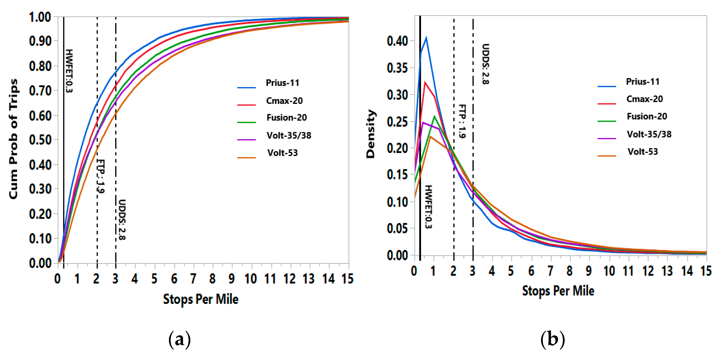
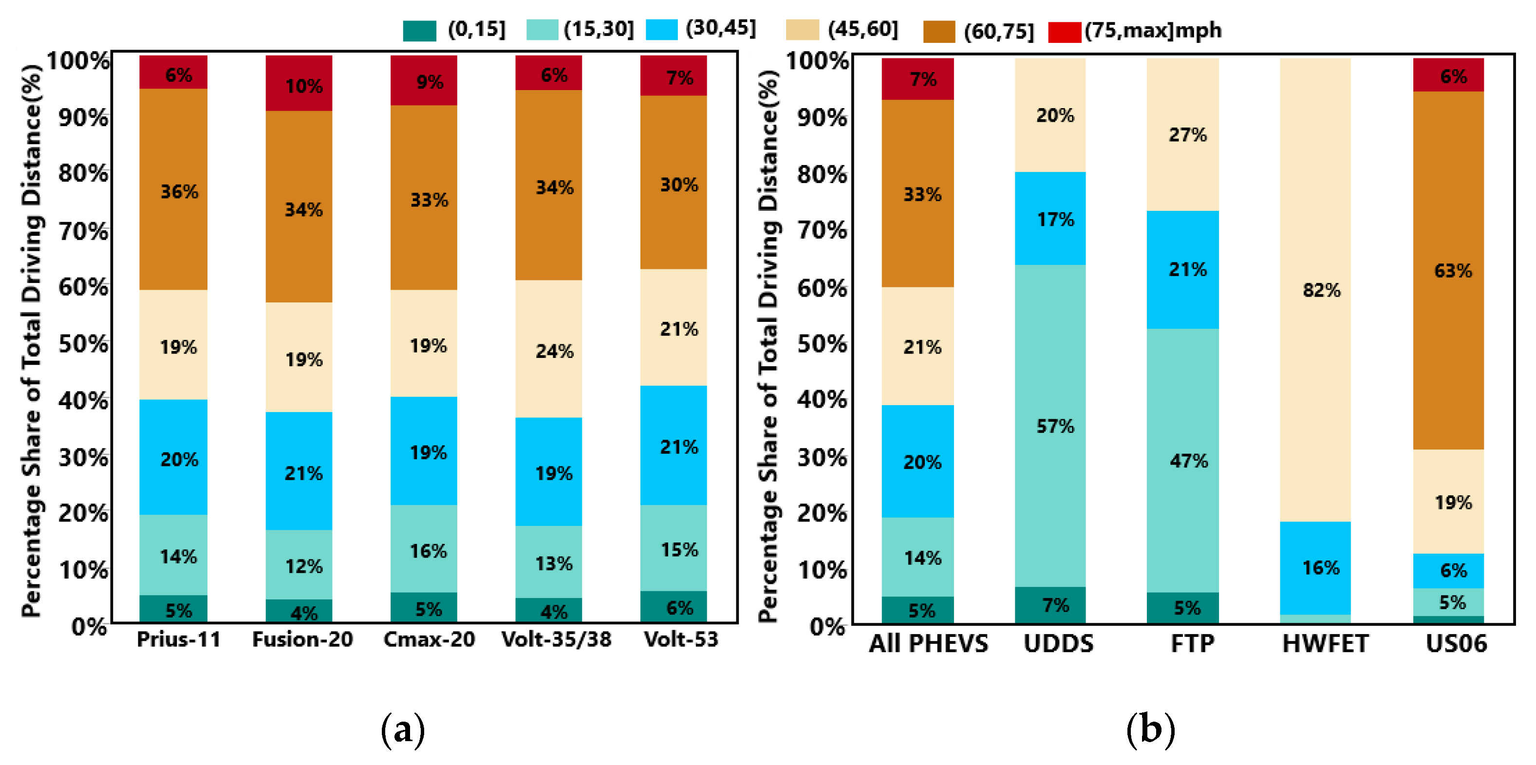
Observed PHEVs are driven more aggressively and accomplish a higher share of travel in non-urban driving conditions (45 mph or faster or less than 3 stops per mile) compared to standardized dynamometer test cycles. The percentage share of time and distance traveled at highway speeds (60 mph or faster) is noticeably under-represented or excluded in test cycles. Approximately 80% of VMT in the UDDS cycle is at 45 mph or slower, whereas the overall average in our dataset was only 40%. Short-range PHEVs (Prius, CMax and Fusion) are driven 4% to 7% more at 60 mph or faster compared to longer-range PHEVs (Volts). The above disparities clearly manifested in the form of increased energy consumption in the CD-EV mode, which reduces the effective AER realized on-road. Using PCA, we characterized driving behavior based on 4 factors: vehicle usage intensity, aggressive driving style at highway speeds which increases the energy intensity, preference for long-distance travel, and conservative driving style.

Analysis of charging behavior revealed marked differences between the single, overnight, fully charged assumption of J2841. On average, observed PHEVs (except the Volt-53) charged more than once per day, and the driving distance on days when the PHEV was not charged was more compared to the days on which they charged at least once. Results indicated that short-range PHEVs have a higher share of driving days when they are not charged at all. The possibility of PHEVs to charge away from home, more than once per day, and PHEV being used like a regular HEV are the other notable distinctions between this study and the generalized J2841 assumptions. The differences in charging behavior outlined above are due to charger accessibility by location (home, away, or both), and charger utilization which could be defined based on frequency of charging or duration of charging. These were characterized using four influential factors extracted by the PCA. Regression models and relative importance analysis indicated that for short-range PHEVs (Prius, CMax, and Fusion), higher annual VMT and share of travel at highway speeds contributed the most to the observed UF being lower than label rated estimates, whereas enhanced charging infrastructure at home and while away increases the UF. In the case of the Volts, long-distance travel days (50 miles or more) and share of travel at highway speeds were the primary reason for lowering the observed UF below its label rated estimated, and increasing the frequency of charging at home increases the UF.

Driving related differences could due to a combination of road infrastructure, early adopter preferences, and vehicle technology attributes like age, AER, maximum electric speed, and drivetrain design. California has the third highest rural interstate and the highest urban interstate highway system length [73], which was partly reflected in the relatively bigger share of highway speed driving observed in this study, compared to test cycles that are used in performance evaluation. California also scores low in proximity to major roadways [74] and ranks among the top three states by average VMT in urban and suburban census tract groups [75]. The cumulative effect of these California specific features were clearly revealed annual VMT and share of long-distance travel (50 miles or more) of the PHEVs observed in this study. The sub-sample of drivers in this dataset are PEV early adopters who purchased or leased a new PHEV and are generally more educated, wealthier, and own a home, compared to mainstream ICE user’s driving patterns in the NHTS on which the J2841 relies on [76,77]. Rebound effect in the classical sense by which improvements in fuel economy of newer vehicles increase the travel demand [78], could also have played a part in higher vehicle usage intensity of all the PHEV models compared to sticker label annual mileage of 15,000 miles, except the Volt-53, which seemed to have faced a slight backfire effect [79].

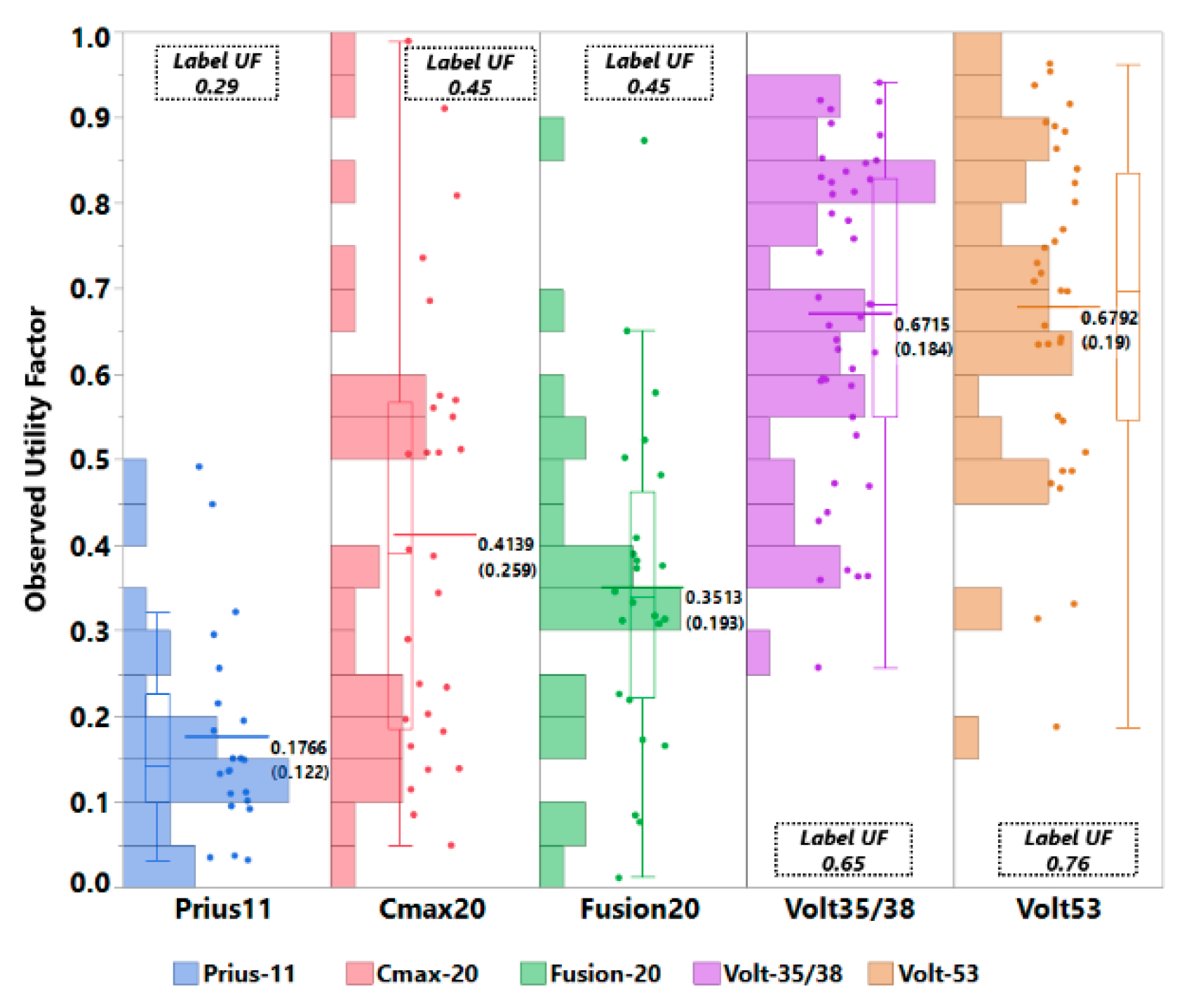
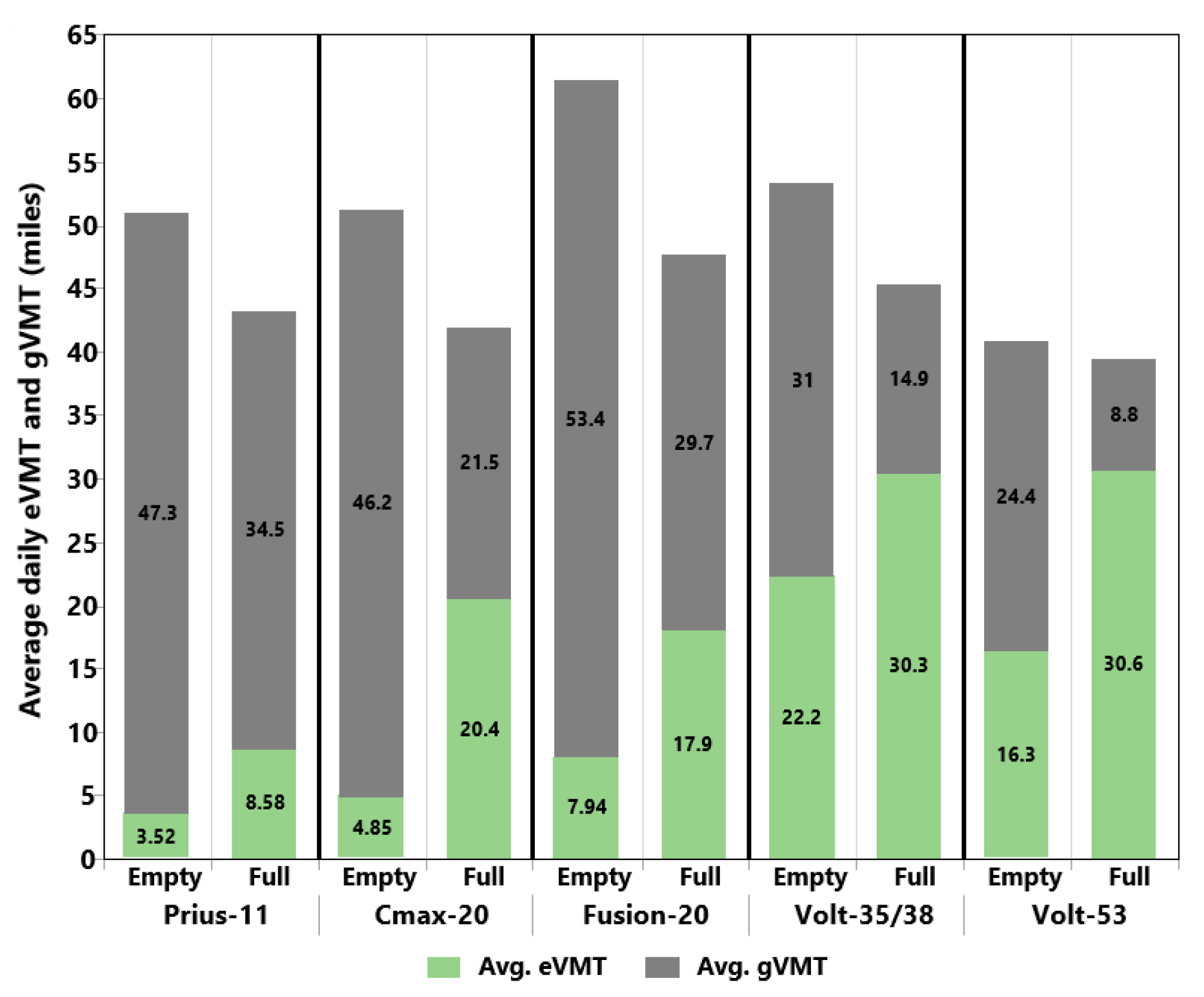
Apart from differences among the PHEV models in terms of annual VMT, driving style (aggressive or conservative), and the magnitude of long-distance travel, the distribution of UF (Figure 1) indicates that heterogeneity in charging preferences exists among different as well as within the same PHEV model. The fact that some PHEVs, irrespective of AER, electrified less than 20% of their rated label UF demonstrates that motivations for charging or not charging are far more complex in reality compared to the simplistic notion of one fully charged session per day at home. Our study illustrates that charger accessibility and utilization have varying levels of influence on the UF depending on the AER. In the case of short-range (20 miles or less, Prius, CMax and Fusion), since their AER is less than their average daily VMT (about 46 miles), there was not enough incentive in the form of eVMT gained, to charge more for compensating their higher travel demand. Lower UF of observed PHEVs compared to their rated label estimates could also be due to self-selection bias by PHEV buyers who are less concerned about eVMT because their decision to purchase the PHEV was motivated by other reasons such as rebate, clean air vehicle decals, or preferential parking spaces. It is also evident that there are diminishing marginal returns in UF and eVMT with an increase in the AER, the case in point being the UF of Volt-53, which was similar to that of Volt-35/38, in spite of the Volt-35/38 driving 2000 miles more than Volt-53 annually.

The performance of PHEVs depends on the intertwined relationships between driving behavior, charging behavior, vehicle technology attributes, and user preferences. The dual propulsion energy source (electric motor and conventional ICE) enables the automakers to offer a wide range of design options to potential buyers depending on the degree of emphasis of one driving mode over the other, which is influenced by the policy goals. Fuel economy and energy efficiency of the ICE were prioritized over the all-electric mode operation due to cost and charging infrastructure considerations in the infant stages of the PHEV market. To maximize the GHG reduction potential of PHEVs, policies that encourage longer-range PHEVs which emphasize more on all-electric mode are needed. While this has a direct impact on the policy signals sent to the automakers and subsequently the model offerings available for potential PHEV buyers, it is critical to consider aspects outside the domain of vehicle technology such as charging infrastructure expansion and heterogeneous user preferences. Though this study does not advocate moving away or replacing the J2841 UF as the metric to quantify the environmental impact of PHEVs, there is definitely room for improving the accuracy UF estimates by incorporating additional scenarios that are more representative of real-world driving and charging behavior.

Generalizability and applicability of this paper’s insights to the broader PHEV market in general, or even within California, is not feasible due to sample size limitations, which is very common and unavoidable, and intrinsic to real-world observational studies. Moreover, today’s PHEV users are early adopters, whose socio-demographic and economic indicators differ from the general population of mainstream ICE users [43]. In essence, results presented in this paper should be interpreted within developmental phases of the PHEV market.

5. Conclusions and Future Research Directions

This study systematically analyzed the driving and charging patterns of 153 PHEVs operating in California. The purpose of this study was to investigate why the observed performance of PHEVs deviated from their expectations and what the influential factors were that contributed to these disparities. We first compared observed and expected PHEV usage patterns.. We also compared the usage patterns of the five PHEV models (Prius, CMax/Fusion Energi, first and second generation Chevrolet Volts) that were analyzed in this study at time-scales varying from trip-level to annual estimates. We utilized principal components analysis to reduce the dimensionality of the dataset while capturing at least 87% of the variance in dataset using just four driving and four charging related factors. The explanatory power and the statistical significance of the extracted factors were evaluated using multivariate regression models. We quantified the relative contribution of each of the extracted factors toward the difference in observed Utility Factor from label expected values. We also investigated if there are any statistically significance interaction terms which further improve the regression model fit and offer additional insights.

Results indicated that higher annual mileage and higher energy intensity were the top two aspects that lowered the observed UF of short-range PHEVs (Prius, CMax/Fusion) when compared to label expectations. Enhanced charging infrastructure access and balanced utilization at home and away increased the observed UF of short-range PHEVs. In the case of longer-range PHEVs (Volts), their propensity toward more long-distance travel (50 or more miles/day), followed by their annual mileage, contributed the most to lowering their UF from label values. Due to their bigger battery capacity, increasing the frequency of shallow charging sessions had a bigger and positive effect on UF, rather than charging for a longer duration time, but less frequently. Regression models indicated that the effect of long-distance travel and deep cycle charging at home were statistically significant for longer-range PHEVs, but not for short-range PHEVs. Analyses also indicated the absence of any statically significant interaction terms. Distribution of UF (Figure 1 and Figure 2) indicated that even within PHEVs with the same AER, there was a diversity in usage patterns. Daily driving distances and style (Figure 2, Figure 3, Figure 4 and Figure 5), number of charging sessions on days driven (Figure 8), and charging location distance from home (Figure 10) demonstrated the linkage between travel and charging behavior and AER.

Plug-in electric vehicles (BEVs and PHEVs) are essential to reduce transport sector GHG emission and energy consumption. Plug-in hybrid electric vehicles are considered to be an intermediate and enabling technology option that can catalyze large-scale adoption of PEVs. The environmental benefits of BEVs are unambiguous due to their zero tail pipe emissions, however the same cannot be said of the PHEVs. Operational and fuel-use flexibility helps the PHEVs in overcoming range anxiety related issues associated with BEVs, but the same flexibility complicates the task of evaluating their net environmental impact. To address this, the concept of UF has been developed and widely utilized in the policy domain and techno-economic assessments. There is a growing body of demonstrable evidence suggesting that a mismatch or gap exists between official EPA sticker label and real-world UF, which warrants a deeper examination to improve our understanding of the electrification potential of PHEVs. This paper focused on this research need by scrutinizing real-world PHEV usage patterns and discerning salient facets of driving and charging that deviated from assumptions embodied in sticker label energy consumption and UF estimates.

Superimposing a set of preconceived notions about driving and charging behavior has direct ramifications on how PHEVs are evaluated in command and control policies like the ZEV mandate, regulations governing their on-road performance, and policies that encourage their usage through economic incentives. Developments in battery technologies, diversification of PHEV model offerings, expansion of charging infrastructure, and a favorable policy environment will increase the market share of PHEVs. As the PHEV market evolves and grows, the need for observing PHEV through studies such as the one presented in this paper will become increasingly valuable. Recognizing real-world scenarios that diverged from assumptions will better inform future policies.

The data collection is still ongoing and future work will include newer PHEV models such as the Chrysler Pacifica Hybrid (33-mile AER) and Toyota Prius Prime (25-mile AER). Future research will incorporate spatio-temporal aspects to identify trip level variables that affect decision to charge or not charge, identify missed charging opportunities at public charging locations, and its implications on the net environmental impact (driving and charging) and electrification potential of PHEVs.

References

1. U.S. Environmental Projection Agency (EPA). Inventory of U. S. Greenhouse Gas Emissions and Sinks: 1990–2017; April 11, 2019, EPA 430-R-19-001; EPA: Washington, DC, USA, 2017.
2. California Air Resources Board (CARB). California Greenhouse Gas Emissions for 2000 to 2017. Trends of Emissions and Other Indicators; CARB: Sacramento, CA, USA, 2017.
3. California Air Resources Board (CARB). California’s Advanced Clean Cars Midterm Review; CARB: Sacramento, CA, USA, 2017.
4. Wang, N.; Tang, L.; Pan, H. A global comparison and assessment of incentive policy on electric vehicle promotion. Sustain. Cities Soc. 2019, 44, 597–603. [Google Scholar] [CrossRef]
5. Lutsey, N. Transition to a Global zero-Emission Vehicle Fleet: A Collaborative Agenda for Governments. 2015. Available online: https://theicct.org/sites/default/files/publications/ICCT_GlobalZEVAlliance_201509.pdf (accessed on 1 August 2019).
6. Poullikkas, A. Sustainable options for electric vehicle technologies. Renew. Sustain. Energy Rev. 2015, 41, 1277–1287. [Google Scholar] [CrossRef]
7. Cordera, R.; dell’Olio, L.; Ibeas, A.; Ortúzar, J.D.D. Demand for environmentally friendly vehicles: A review and new evidence. Int. J. Sustain. Transp. 2019, 13, 210–223. [Google Scholar] [CrossRef]
8. Society of Automotive Engineers (SAE). J1711_201006: Recommended Practice for Measuring the Exhaust Emissions and Fuel Economy of Hybrid-Electric Vehicles, Including Plug-in Hybrid Vehicles; SAE International: Warrendale, PA, USA, 2010. [Google Scholar]
9. Society of Automotive Engineers (SAE). J2841_201009: Utility Factor Definitions for Plug-In Hybrid Electric Vehicles Using Travel Survey Data; SAE International: Warrendale, PA, USA, 2010. [Google Scholar] [CrossRef]
10. U.S. Environmental Protection Agency (EPA). Dynamometer Drive Schedules. Available online: https://www.epa.gov/vehicle-and-fuel-emissions-testing/dynamometer-drive-schedules (accessed on 10 October 2018).
11. CARB. California’s Advanced Clean Cars Midterm Review, Appendix H: Plug-in Hybrid Electric Vehicle Emissions Testing; CARB: Sacramento, CA, USA, 2017.
12. Hu, P.S.; Reuscher, T.R. Summary of Travel Trends: 2001 National Household Travel Survey. 2004. Available online: http://nhts.ornl.gov/2001/pub/STT.pdf (accessed on 10 October 2018).
13. Bradley, T.H.; Davis, B.M. Alternative Plug in Hybrid Electric Vehicle Utility Factor; 0148-7191; SAE Technical Paper: Warrendale, PA, USA, 2011. [Google Scholar]
14. Bradley, T.H.; Quinn, C.W. Analysis of plug-in hybrid electric vehicle utility factors. J. Power Sources 2010, 195, 5399–5408. [Google Scholar] [CrossRef]
15. Brady, J.; O’Mahony, M. Development of a driving cycle to evaluate the energy economy of electric vehicles in urban areas. Appl. Energy 2016, 177, 165–178. [Google Scholar] [CrossRef]
16. Wu, X.; Aviquzzaman, M.; Lin, Z. Analysis of plug-in hybrid electric vehicles’ utility factors using GPS-based longitudinal travel data. Transp. Res. Part C Emerg. Technol. 2015, 57, 1–12. [Google Scholar] [CrossRef]
17. Karabasoglu, O.; Michalek, J. Influence of driving patterns on life cycle cost and emissions of hybrid and plug-in electric vehicle powertrains. Energy Policy 2013, 60, 445–461. [Google Scholar] [CrossRef]
18. Neubauer, J.; Brooker, A.; Wood, E. Sensitivity of plug-in hybrid electric vehicle economics to drive patterns, electric range, energy management, and charge strategies. J. Power Sources 2013, 236, 357–364. [Google Scholar] [CrossRef]
19. Björnsson, L.-H.; Karlsson, S.; Sprei, F. Objective functions for plug-in hybrid electric vehicle battery range optimization and possible effects on the vehicle fleet. Transp. Res. Part C Emerg. Technol. 2018, 86, 655–669. [Google Scholar] [CrossRef]
20. Tamor, M.A.; Gearhart, C.; Soto, C. A statistical approach to estimating acceptance of electric vehicles and electrification of personal transportation. Transp. Res. Part C Emerg. Technol. 2013, 26, 125–134. [Google Scholar] [CrossRef]
21. Smart, J.; Bradley, T.; Salisbury, S. Actual versus estimated utility factor of a large set of privately owned Chevrolet Volts. SAE Int. J. Altern. Powertrains 2014, 3, 30–35. [Google Scholar] [CrossRef]
22. Smart, J.; Powell, W.; Schey, S. Extended Range Electric Vehicle Driving and Charging Behavior Observed Early in the EV Project; 0148-7191; SAE Technical Paper: Warrendale, PA, USA, 2013. [Google Scholar]
23. Duhon, A.N.; Sevel, K.S.; Tarnowsky, S.A.; Savagian, P.J. Chevrolet volt electric utilization. Sae Int. J. Altern. Powertrains 2015, 4, 269–276. [Google Scholar] [CrossRef]
24. Plötz, P.; Funke, S.Á.; Jochem, P. Empirical Fuel Consumption and CO2 Emissions of Plug-In Hybrid Electric Vehicles. J. Ind. Ecol. 2018, 22, 773–784. [Google Scholar] [CrossRef] [Green Version]
25. Ensslen, A.; Ringler, P.; Dörr, L.; Jochem, P.; Zimmermann, F.; Fichtner, W. Incentivizing smart charging: Modeling charging tariffs for electric vehicles in German and French electricity markets. Energy Res. Soc. Sci. 2018, 42, 112–126. [Google Scholar] [CrossRef]
26. Clairand, J.-M.; Rodríguez-García, J.; Álvarez-Bel, C. Smart charging for electric vehicle aggregators considering users’ preferences. IEEE Access 2018, 6, 54624–54635. [Google Scholar] [CrossRef]
27. Chung, H.-M.; Li, W.-T.; Yuen, C.; Wen, C.-K.; Crespi, N. Electric vehicle charge scheduling mechanism to maximize cost efficiency and user convenience. IEEE Trans. Smart Grid 2018, 10, 3020–3030. [Google Scholar] [CrossRef] [Green Version]
28. California Air Resources Board (CARB). California’s Advanced Clean Cars Midterm Review; Appendix G, H I; CARB: Sacramento, CA, USA, 2017.
29. U.S. Environmental Protection Agency (EPA). Special Procedures Related to Electric Vehicles and Hybrid Electric Vehicles; 40, FR 39548, 6 July 2011, as Amended at 76 FR 57380, 15 September 2011; EPA: Washington, DC, USA, 2011; Volume 76.
30. EIA. Analysis of the Effect of Zero-Emission Vehicle Policies: State Level Incentives and the California Zero-Emission Vehicle Regulations; EIA: Washington, DC, USA, 2017.
31. Allen, P.; Van Horn Vermeer, G. California’s Light-Duty Vehicle Emissions Standards: The Clean Air Act Waiver, Standards History, and Current Status; MJ Bradley & Associates Issue Brief: Concord, MA, USA, 2017; pp. 1–7. [Google Scholar]
32. Duoba, M. Design of an On-Road PHEV Fuel Economy Testing Methodology with Built-In Utility Factor Distance Weighting. Sae Int. J. Altern. Powertrains 2012, 1, 349–353. [Google Scholar] [CrossRef]
33. Gonder, J.; Brooker, A.; Carlson, R.B.; Smart, J. Deriving in-use PHEV fuel economy predictions from standardized test cycle results. In Proceedings of the IEEE Vehicle Power and Propulsion Conference, Dearborn, MI, USA, 7–10 September 2009; pp. 643–648. [Google Scholar]
34. Farrell, A.E.; Sperling, D.; Arons, S.; Brandt, A.; Delucchi, M.; Eggert, A.; Farrell, A.; Haya, B.; Hughes, J.; Jenkins, B.; et al. A Low-Carbon Fuel Standard for California Part 1: Technical Analysis; UCB-ITS-TSRC-RR-2007-3; UC Berkeley: Berkeley, CA, USA, 2007. [Google Scholar]
35. Aviquzzaman, M. Analysis of Plug-In Hybrid Electric Vehicles’ Utility Factors Using GPS-Based Longitudinal Travel Data; Lamar University-Beaumont: Beaumont, TX, USA, 2014. [Google Scholar]
36. Stephens, T.S.; Levinson, R.S.; Brooker, A.; Liu, C.; Lin, Z.; Birky, A.; Kontou, E. Comparison of Vehicle Choice Models; Argonne National Lab. (ANL): Argonne, IL, USA; Sandia National Lab. (SNL-NM): Albuquerque, NM, USA; National Renewable Energy Lab. (NREL): Golden, CO, USA; Oak Ridge National Lab. (ORNL): Oak Ridge, TN, USA, 2017.
37. Kim, N.; Duoba, M.; Kim, N.; Rousseau, A. Validating Volt PHEV model with dynamometer test data using Autonomie. Sae Int. J. Passeng. Cars Mech. Syst. 2013, 6, 985–992. [Google Scholar] [CrossRef]
38. McCollum, D.L.; Wilson, C.; Pettifor, H.; Ramea, K.; Krey, V.; Riahi, K.; Bertram, C.; Lin, Z.; Edelenbosch, O.Y.; Fujisawa, S. Improving the behavioral realism of global integrated assessment models: An application to consumers’ vehicle choices. Transp. Res. Part D Transp. Environ. 2017, 55, 322–342. [Google Scholar] [CrossRef]
39. Wood, E.W.; Rames, C.L.; Bedir, A.; Crisostomo, N.; Allen, J. California Plug-In Electric Vehicle Infrastructure Projections: 2017–2025-Future Infrastructure Needs for Reaching the State’s Zero Emission-Vehicle Deployment Goals; National Renewable Energy Lab. (NREL): Golden, CO, USA, 2018.
40. U.S. Environmental Protection Agency (EPA); California Air Resources Board (CARB). EMFAC Emissions Model; EPA: Washington, DC, USA; CARB: Sacramento, CA, USA, 2018.
41. Tal, G.; Raghavan, S.; Karanam, V.; Favetti, M.; Sutton, K.; Lee, J.H.; Nitta, C.; Chakraborty, D.; Nicholas, M.; Turrentine, T. Advanced Plug-in Electric Vehicle Travel and Charging Behavior -Final Report; California Air Resources Board Contract #12-319(Under Review): Sacramento, CA, USA, 2019.
42. Turrentine, T.; Tal, G. Advanced Plug-In Electric Vehicle Usage and Charging Behavior; Contract #12-319. California Air Resources Board (CARB); California Energy Commission (CEC): Washington, DC, USA, 2015.
43. Center for Sustainable Energy. Clean Vehicle Rebate Project, Final Report Fiscal Year 2014–2015, Center for Sustainable Energy. Prepared under Grant G14-AQIP-01 for the California Air Resources Board; Center for Sustainable Energy: San Diego, CA, USA, 2016. [Google Scholar]
44. Environmental Protection Agency (EPA). Fuel Economy Labeling of Motor Vehicles; EPA: Washington, DC, USA, 2006; Volume 71, pp. 77871–77969.
45. Society of Automotive Engineers (SAE). J1772_201710: Electric Vehicle and Plug in Hybrid Electric Vehicle Conductive Charge Coupler; SAE International: Warrendale, PA, USA, 2017. [Google Scholar] [CrossRef]
46. U.S. EPA. Fuel Economy Data. Available online: https://www.fueleconomy.gov/feg/download.shtml (accessed on 1 May 2019).
47. Kaiser, H.F.; Rice, J. Little jiffy, mark IV. Educ. Psychol. Meas. 1974, 34, 111–117. [Google Scholar] [CrossRef]
48. Kaiser, H.F. A second generation little jiffy. Psychometrika 1970, 35, 401–415. [Google Scholar] [CrossRef]
49. Tobias, S.; Carlson, J.E. Brief report: Bartlett’s test of sphericity and chance findings in factor analysis. Multivar. Behav. Res. 1969, 4, 375–377. [Google Scholar] [CrossRef] [PubMed]
50. Cerny, B.A.; Kaiser, H.F. A study of a measure of sampling adequacy for factor-analytic correlation matrices. Multivar. Behav. Res. 1977, 12, 43–47. [Google Scholar] [CrossRef] [PubMed]
51. Kaiser, H.F. An index of factorial simplicity. Psychometrika 1974, 39, 31–36. [Google Scholar] [CrossRef]
52. Chan, L.L.; Idris, N. Validity and Reliability of The Instrument Using Exploratory Factor Analysis and Cronbach’s alpha. Int. J. Acad. Res. Bus. Soc. Sci. 2017, 7, 400–410. [Google Scholar]
53. Hair, J.F.; Black, W.C.; Babin, B.J.; Anderson, R.E.; Tatham, R.L. Multivariate Data Analysis; Pearson Prentice Hall: Upper Saddle River, NJ, USA, 2006; Volume 6. [Google Scholar]
54. Salkind, N.J. Encyclopedia of Research Design; Sage: Thousand Oaks, CA, USA, 2010; Volume 2. [Google Scholar]
55. Yong, A.G.; Pearce, S. A beginner’s guide to factor analysis: Focusing on exploratory factor analysis. Tutor. Quant. Methods Psychol. 2013, 9, 79–94. [Google Scholar] [CrossRef]
56. Schmitt, T.A.; Sass, D.A. Rotation criteria and hypothesis testing for exploratory factor analysis: Implications for factor pattern loadings and interfactor correlations. Educ. Psychol. Meas. 2011, 71, 95–113. [Google Scholar] [CrossRef]
57. Osborne, J.W.; Costello, A.B.; Kellow, J.T. Best practices in exploratory factor analysis. In Best Practices in Quantitative Methods; Sage: Thousand Oaks, CA, USA, 2008; pp. 86–99. [Google Scholar]
58. Jolliffe, I.T.; Cadima, J. Principal component analysis: A review and recent developments. Philos. Trans. R. Soc. A Math. Phys. Eng. Sci. 2016, 374, 20150202. [Google Scholar] [CrossRef]
59. Grömping, U. Estimators of relative importance in linear regression based on variance decomposition. Am. Stat. 2007, 61, 139–147. [Google Scholar] [CrossRef]
60. Tonidandel, S.; LeBreton, J.M.; Johnson, J.W. Determining the statistical significance of relative weights. Psychol. Methods 2009, 14, 387. [Google Scholar] [CrossRef]
61. Tonidandel, S.; LeBreton, J.M. Relative importance analysis: A useful supplement to regression analysis. J. Bus. Psychol. 2011, 26, 1–9. [Google Scholar] [CrossRef]
62. Boston, D.; Werthman, A. Plug-in vehicle behaviors: An analysis of charging and driving behavior of ford plug-in electric vehicles in the real world. World Electr. Veh. J. 2016, 8, 926–935. [Google Scholar] [CrossRef] [Green Version]
63. EPA, U.S. Title 40-Protection of Environment. Fuel Economy and Greenhouse Gas Exhaust Emissions of Motor Vehicles. Special procedures related to electric vehicles and hybrid electric vehicles. In 40 CFR § 600.116-12; Title 40, Subchapter Q, Part 600; EPA: Washington, DC, USA, 2019; Chapter I.
64. California Air Resources Board (CARB). California Air Resources Board Zero Emission Vehicle Program; CARB: Sacramento, CA, USA, 2016.
65. Bureau of Transportation Statistics (BTS). Long Distance Transportation Patterns: Mode Choice. Available online: https://www.bts.gov/statistical-products/surveys/national-household-travel-survey-summer-travel-quick-facts (accessed on 15 July 2018).
66. Wesseling, J.; Niesten, E.; Faber, J.; Hekkert, M. Business strategies of incumbents in the market for electric vehicles: Opportunities and incentives for sustainable innovation. Bus. Strategy Environ. 2015, 24, 518–531. [Google Scholar] [CrossRef] [Green Version]
67. Kaiser, H.F. The application of electronic computers to factor analysis. Educ. Psychol. Meas. 1960, 20, 141–151. [Google Scholar] [CrossRef]
68. Faul, F.; Erdfelder, E.; Lang, A.-G.; Buchner, A. G* Power 3: A flexible statistical power analysis program for the social, behavioral, and biomedical sciences. Behav. Res. Methods 2007, 39, 175–191. [Google Scholar] [CrossRef] [PubMed]
69. Fritz, M.S.; MacKinnon, D.P. Required sample size to detect the mediated effect. Psychol. Sci. 2007, 18, 233–239. [Google Scholar] [CrossRef] [Green Version]
70. Champoux, J.E.; Peters, W.S. Form, effect size and power in moderated regression analysis. J. Occup. Psychol. 1987, 60, 243–255. [Google Scholar] [CrossRef]
71. Cohen, J. Statistical Power Analysis for the Behavioral Sciences, 2nd ed.; Erlbaum: Hillsdale, NJ, USA, 1988. [Google Scholar]
72. Saltelli, A. Making best use of model evaluations to compute sensitivity indices. Comput. Phys. Commun. 2002, 145, 280–297. [Google Scholar] [CrossRef]
73. Federal Highway Administration (FHWA). National Highway System Length; FHWA: Washington, DC, USA, 2018.
74. U.S. Department of Transportation (DOT). Transportation and Health Tool; DOT: Washington, DC, USA, 2016.
75. Santos, A.; McGuckin, N.; Nakamoto, H.Y.; Gray, D.; Liss, S. Summary of Travel Trends: 2009 National Household Travel Survey. 2011. Available online: http://nhts.ornl.gov/2009/pub/stt.pdf (accessed on 15 July 2018).
76. Tal, G.; Dunckley, J. Plug-In Electric Vehicle Multi-State Market and Charging Survey; 3002007495; EPRI (Electric Power Research Institute): Palo Alto, CA, USA, 2016. [Google Scholar]
77. Tal, G.; Nicholas, M.A.; Woodjack, J.; Scrivano, D. Who is Buying Electric Cars in California? Exploring Household and Vehicle Fleet Characteristics of New Plug-In Vehicle Owners; UCD-ITS-RR-13-02; UC Davis: Davis, CA, USA, 2013. [Google Scholar]
78. Leard, B.; Linn, J.; Munnings, C. Explaining the evolution of passenger vehicle miles traveled in the United States. Energy J. 2019, 40. [Google Scholar] [CrossRef] [Green Version]
79. Gillingham, K.; Kotchen, M.J.; Rapson, D.S.; Wagner, G. Energy policy: The rebound effect is overplayed. Nature 2013, 493, 475. [Google Scholar] [CrossRef]
Figure 1. Distribution of individual Utility Factor (UF) by PHEV model. Average and standard deviation of UF is indicated within parentheses. EPA label city/highway combined UF is shown inset.
Wevj 11 00006 g001
Figure 2. Ratio of observed Utility Factor (UF) to EPA label city/highway combined UF by PHEV model. Values above one indicates observed UF of PHEVs exceeded EPA estimates.
Wevj 11 00006 g002
Figure 3. Percentage share of total driving time by driving speed in mph: (a) Observed PHEVs; (b) Comparison with EPA Test Cycles.
Wevj 11 00006 g003
Figure 4. Distribution of stops per mile. (a) Cumulative distribution function (CDF); (b) Density plot. Vertical lines are drawn to indicate representative highway and urban drive cycles stops per mile.
Wevj 11 00006 g004
Figure 5. Percentage share of total driving distance by driving speed in mph: (a) Observed PHEVs; (b) Comparison with EPA Test Cycles.
Wevj 11 00006 g005
Figure 6. Distribution of real-world fuel economy (MPG) in CS mode trips and electricity consumption in CD-EV or ZE mode (kWh/mile) trips. In the ZE mode the engine was never turned on and CS trips was accomplished entirely on gasoline. Values adjacent to the solid dashed line show the average and standard deviation.
Wevj 11 00006 g006
Figure 7. Percentage share of total VMT by distance traveled on weekdays and weekends.
Wevj 11 00006 g007
Figure 8. Percentage share of driven days by number of charging sessions on weekdays and weekends.
Wevj 11 00006 g008
Figure 9. Impact of Travel Day Starting SOC on Average daily eVMT and gVMT.
Wevj 11 00006 g009
Figure 10. Percentage share of L1 and L2 charging sessions by distance from home. Values less than or equal to 1% have been omitted for clarity. Distances are the great-circle distances calculated using the Haversine formula.
Wevj 11 00006 g010