The Influence of Electric Vehicle Charging on Low Voltage Grids with Characteristics Typical for Germany

Abstract

The increasing number of electric vehicles poses new challenges to the power grid. Their charging process stresses the power system, as additional energy has to be supplied, especially during peak load periods. This additional load can result in critical network situations depending on various parameters. These impacts may vary based on market penetration, the energy demand, the plug-in time, the charging rate, and the grid topology and the associated operational equipment. Hence, the impact of electric vehicles (EVs) on the power grid was analysed for twelve typical German low voltage grids by applying power flow calculations. One main result was that thermal and voltage-related network overloads were highly dependent on market penetration and grid topology.

1. Introduction

In the current automotive sector, there is a strong trend towards the electrification of the power train [1]. However, an increase in market penetration of electric vehicles (EVs) can pose new challenges to the power grid, as additional energy has to be supplied for the charging processes, and the corresponding EV load is relatively high compared to other domestic applications. Since EVs are mainly connected to the low voltage (LV) distribution grid, the main problems are expected for this grid [2,3,4]. The additional loads can affect the grid and jeopardise network stability [5]. Possible network effects include decreasing power quality, power losses, deterioration of infrastructure (by exceeding thermal limits of feeders, etc.), and line congestion [6,7]. Due to the heterogeneity of the LV grids and the regionally different LV grid topologies, different impacts can be expected depending on the region [8].

However, the resulting grid impacts are also strongly dependent on the spatial market penetration, the charging rates, plug-in time, the grid structure, and the corresponding operating equipment in the power grid [9]. Furthermore, the individual charging and mobility behaviour of EV users is a significant influencing factor [10,11]. Consequently, the following research questions emerged:

• What are the impacts on the grids caused by an increasing market penetration of EV?
• Are there substantial regional differences in distribution grid topologies which are relevant for EV charging?
• How decisive is the individual charging behaviour of EV users and the resulting simultaneity of the charging processes in grid analysis?

The scope of this publication is to investigate various low voltage distribution grids and give an overview of the impacts of EV charging on German low voltage grids. In special cases (e.g., exceptional grid structures), significant differences are expected. Hence, in this contribution, various low voltage grids that present typical regional differences in the grid topology, and different population densities and agglomerations are considered. A preliminary version of this article was presented at the EVS32 Symposium, Lyon, France, 20–22 May 2019 [12]. In addition to the publication at EVS32, further low voltage grids were investigated; [12] was extended by taking into account unbalanced charging, adding in-depth analysis, and doing a detailed presentation and interpretation of results.

This paper is organised as follows. In Section 2, reference grids are identified based on different regional structural data. All relevant parameters are identified. Section 3 gives an overview of the valid regulations for grid operation in Germany. Then, the simultaneity factor is introduced and differences in its calculations for different grid limits are explained in Section 4. The determination of the energy demands of EVs and households in this publication will be explained in Section 5. Section 6 gives an overview of the scenarios considered. Based on the low voltage distribution grids and the simultaneity factor in Section 7, the influence of EV charging on different types of low voltage grids is considered and the results are compared. A summary and outlook conclude the paper.

2. Low Voltage Grids

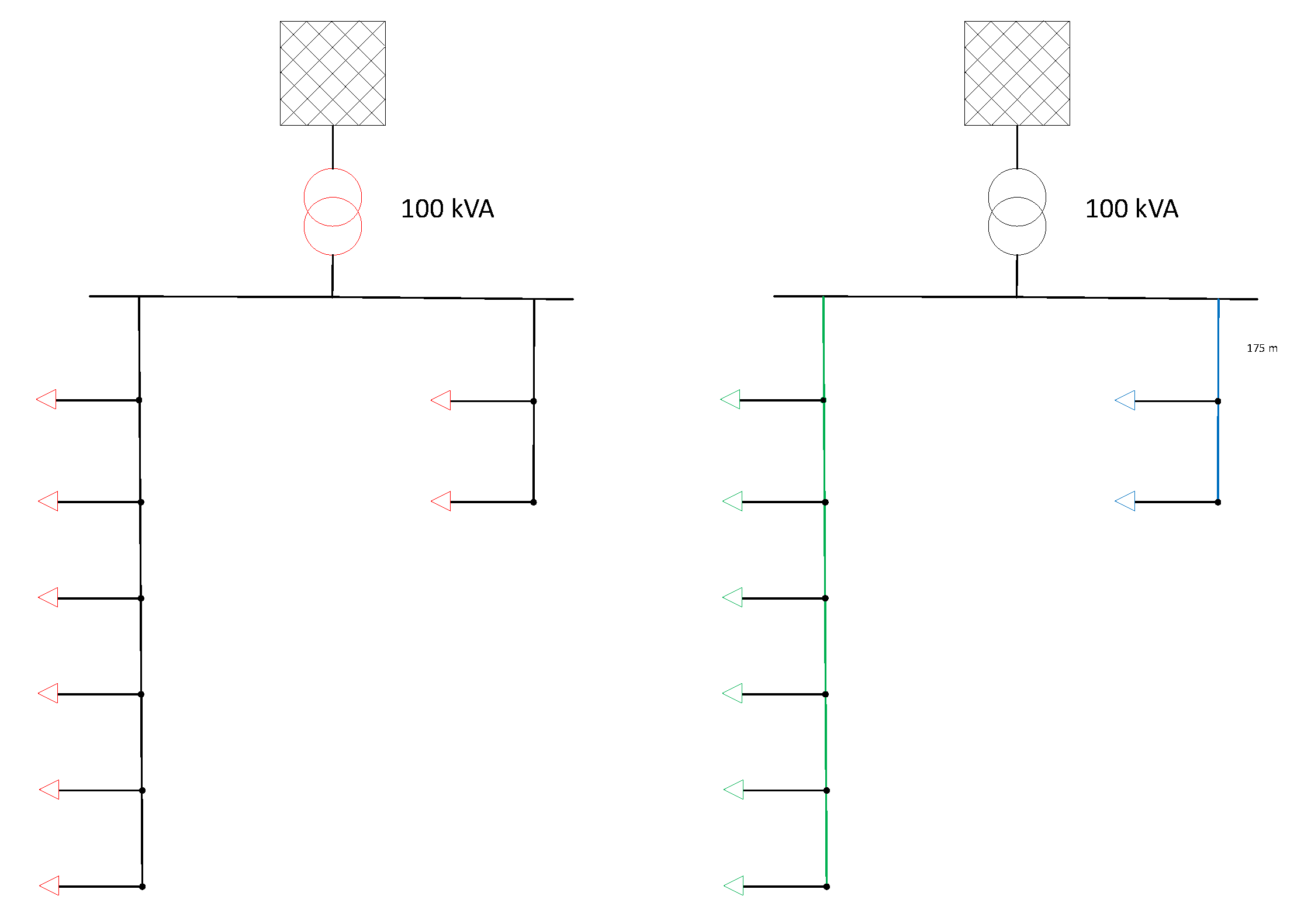
2.1. Low Voltage Test Grids

Low voltage grids differ significantly regarding their dimensions and technical performances. In [13], 86 existing German low voltage grids were analysed in detail and typical grid structures were identified. Representative grids were developed using these data. Each grid is typical for a specific population density and agglomeration (e.g., rural or urban areas). In total, the twelve grids that are described in

Table 1. Overview of the typical German low voltage grid.

Grid Name	Description
Campestral Grid 1	Represents a typical grid for a campestral area.
Campestral Grid 2	Represents an additional typical grid for a campestral area. In comparison to Campestral Grid 1, another transformer is used here and the grid structure is different.
Campestral Grid 3	This grid is a campestral grid with an extremely long feeder.
Campestral Grid 4	Campestral Grid 4 has a similar structure than Campestral Grid 3, but cable type and distance between the households is varied.
Campestral Grid 5	Campestral Grid 5 is similar to Campestral Grid 4, but the nominal power of the transformer is lower as well as additional households are added. Campestral Grid 5 represents a campestral grid with extremely long feeder and highly utilized transformer.
Rural Grid 1	Represents a typical grid for a rural area.
Rural Grid 2	Represents a rural grid with an extremely long feeder.
Rural Grid 3	In comparison to Rural Grid 2, here the nominal power of the transformer is lower as well as additional households exist, so that this grid represents a rural grid with extremely long feeder and a highly utilized transformer.
Suburban Grid 1	Represents a typical grid for a suburban area.
Suburban Grid 2	Represents a typical grid for a suburban area. In comparison to Suburban Grid 1, another cable type is used here.
Suburban Grid 3	This grid represents a typical grid with an extremely long feeder in a suburban area.
Suburban Grid 4	This grid represents a typical grid with an extremely long feeder in a suburban area. In comparison to Suburban Grid 3, another cable type is used here.

, are used in this paper to compare the impact of EV charging on low voltage grids.

In Figure 1, the grid structure of Suburban Grid 1 is presented.

It consists of 153 grid customers in total, which are divided into ten feeders of different length. In comparison to the rural and campestral grid, the number of grid customers is the highest, which is typical for suburban grids. The low voltage grid is connected to the medium voltage (MV) grid via a 630 kVA MV/LV-transformer. In total four different suburban grids were considered within this contribution.

In Figure 2, the grid Rural Grid 1 is shown. Through six feeders, 57 grid customers are connected via a 400 kVA transformer to the MV grid. In this publication, three different grids representative for a rural area are used.

In Figure 3, Campestral Grid 1 is depicted. It consists of only two feeders, including eight grid customers. The length of the feeders in this grid is significantly higher than in the other considered grids. Five different grids representative for a campestral area are investigated in this publication. Urban grids are not considered, as charging of EV at home is less common due to the fact that more people do not own a car or do not have the possibility of charging at home.

For the grid impedance Z, the parameters shown in

Table 2. Grid data.

	R (Ohm/km)	L (mH/km)
NAYY 4 × 150 mm2	0.206	0.256
NAYY 4 × 50 mm2	0.641	0.270

were used. For all vertical lines in Figure 1, Figure 2 and Figure 3, a cable of type NAYY 4 × 150 mm² was used; for the horizontal lines the type was NAYY 4 × 50 mm².

The line length L was set according to [13]. The voltage at the transformer was set to the nominal voltage U_Nominal, which is 1 p.u. (400 V).

2.2. Unbalanced Loading or Charging

In the literature, low voltage grids are often modelled as symmetrical grids (see for instance, [6,10,13]). Hence, it was assumed that the loading or charging processes in the grid were balanced between the different phases in the grid. In reality, this is not the case; for example, many EVs are only charging on one or two phases. In [14] it was shown that the correct allocation to the different phases has significant influence on the results. Therefore, the assumption that all EV are charging balanced is neglected in this paper.

The low voltage grid was modelled as a three-phase grid (phase A, phase B, and phase C) with a neutral line (as low voltage grids are constructed this way in Germany). Additional currents over the ground and mutual couplings between the different phases were also neglected.

For results, the voltages were calculated for each phase separately, as can be seen in Figure 4 for an exemplary power flow with a higher load on phase A than on phase B and C.

Under unbalanced conditions, power is also flowing on the neutral line (phase N) and causing a voltage rise, as can be seen in Figure 5.

The voltage difference between each phase and the neutral line is the voltage provided to the consumer. Hence, this is also the relevant voltage for reviewing the compliance with the given grid limits. The magnitudes of these voltages are displayed in Figure 6. Here, it has to be mentioned that voltage is a complex quantity; consequently, it is not possible to just add the magnitudes that can be seen in Figure 4 and Figure 5.

3. Limits for Grid Operation

In order to ensure network stability, there are grid operating conditions which must be observed. The standard DIN EN 50160/A1:2016-02 [15] defines the valid regulations for grid operation in Germany.

At the interconnection point to end consumers, the maximum voltage deviation must not deviate between ±10% from the nominal voltage [15]. The grid operators split this deviation between the different voltage levels. In this paper, the maximum voltage drop for the LV grid is set to 5% of the nominal voltage. As the voltage at the transformer is set to U_Nominal (1 p.u.), the minimal allowed voltage U_Min,Limit is 0.95 p.u. (380 V).

Additionally, the criterion for voltage unbalance is taken into account. The voltage unbalance is defined as the ratio between the negative sequence voltage V₂ and positive sequence voltage V₁. Following the standard DIN EN 50160/A1:2016-02 [15], the voltage unbalance may not exceed 2%.

$$\frac{V2}{V1}\le 2\%$$

(1)

With regard to the thermal limitation, the nominal capacity of the operational equipment must not be exceeded. This is not part of [15], but has to be taken into account to prevent failure of equipment. Therefore, power limits of transformers and current limits for lines were taken into account in our simulations. Additional equipment (e.g., protection devices) is normally coordinated with the thermal limits of lines and transformers. Hence, an additional review of these thermal limits does not have to be considered.

4. Simultaneity in the Power Demand

The power grid transports and distributes energy to all clients at any time, and hence, the valid limits for grid operation have to always be fulfilled. To check the compliance with the given limits, it is sufficient to consider only extreme points of time. If the limits are fulfilled at these times, they are considered to be fulfilled at all the other times, too. As EVs are an additional load, the high-load scenario is the extreme point of time that is reviewed in this paper. Hence, the resulting peak power of EV charging is of interest.

4.1. The Concept of Simultaneity Factors

Considering several consumers in the power grid, it is not probable that they all show their individual peak power P_Peak at the same time. For example, in the context of this paper, it is not probable that all EVs owners charge their car at the same time with full charging power. Therefore, a simultaneity factor s(n), which depends on the number of involved grid customers n (e.g., car owners), is used to characterise the contribution of each load to the total peak load of the regarded grid area. In previous publications this concept was already adapted for EV charging [6].

For the calculation of the power-flow at high-load times, the power consumed at each load P(n) is calculated using the following formula:

$$P\left(n\right)=s\left(n\right)·P_{\mathrm{Peak}}\forall n.$$

(2)

In comparison to a probabilistic time series based approach, the number of necessary power flow calculations can be reduced significantly using simultaneity factors. For each scenario, only one power flow calculation at the high-load point of time is sufficient. In contrast to that, in a probabilistic approach, a high number of power flow calculations has to be performed to reduce statistical variations. In addition to a time series based approach, additional computation time is needed using a simultaneity factor for the calculation of the factor, but the total computation time is still significantly lower. Besides the active power, the reactive power is also taken into account using a power factor $\cos \theta$ of 0.95 in the following.

4.2. The Calculation of Simultaneity Factors for Different Grid Limits

The number of involved grid connection points n, which is used to calculate the simultaneity factor, depends on the limit for grid operation, which has to be verified. To calculate the utilisation of the transformer (c.f. the left side of Figure 7), the number of involved grid connection points n is equal to all grid connection points in the grid (marked in red in Figure 7), as the energy consumption of each household influences the utilisation of the transformer. To calculate the utilisation of the lines and cables and the voltages in the grid (c.f. the right side of Figure 7), the number of involved grid connection points n is the number of grid customers that are connected to the same feeder (marked in green and blue in Figure 7). Only the energy consumption of a grid connection point in the same feeder influences the power flow, and therefore, the utilisation of a line. Hence, the same statement is valid for the voltage as the voltage is considered constant on the low voltage side of the MV/LV transformer. Consequently, different simultaneity factors have to be used for each feeder depending on the number of grid connection points n in each feeder. Hence, in total two simulations were performed using different simultaneity factors to verify the different limits.

5. Energy Demand of the Households and EVs

The methodology to calculate the simultaneity factors and resulting peak power in this article is related to an open-source software tool [16], that was developed by the authors of this paper. The algorithm we used was presented in detail in [17]. In the following chapter, the basic approach is presented for the calculation of the simultaneity factors for EV charging and the households. A time resolution of 15 min for all time series was used, as the used household profiles are available in this resolution.

5.1. EV Charging

When determining the impact of the charging process on the power grid, the charging power is the decisive factor. The charging power depends on the car model. In 2019, the share of battery electric vehicle (BEV) in plug-in electric vehicle (PEV) was 55.4%; the share of plug-in hybrid electric vehicle (PHEV) was 44.6% [18]. The average charging power for BEV is 11.5 kW and 3.6 kW for PHEV. These are results of an analysis of the charging power for EVs on the German market using data from [19]. Hence, the average charging power P_Char is calculated as given in Equation (3).

$$P_{\mathrm{Char}}=\frac{55.4·11.5\mathrm{kW}+44.6·3.6\mathrm{kW}}{100}\approx 8\mathrm{kW}.$$

(3)

Market penetrations of EV by 0%, 12.5%, 25%, 37.5%, 50%, 62.5%, 75%, 87.5%, 100%, 112.5%, 125%, 137.5%, and 150% were considered in the calculations. Thereby, a penetration of 100% means that exactly one EV is connected to each grid connection point; i.e., one EV per house. In Germany, 82.8 million people [20] live with 41.51 million cars [21]. Considering only people not living in cities (71% of the total inhabitants [22], owning 78.2% of all vehicles [21]) and assuming two inhabitants per household [23] and 1.3 households per house [24], a total conversion from fossil fuel based vehicles to EV would lead to 1.42 EVs per grid connection point.

As mentioned before, we want to calculate the simultaneity in a high-load scenario. Therefore, the daily maximum simultaneity factor is calculated as follows:

• The number of EVs in each low voltage grid is calculated multiplying the number of household with the penetration of EVs. The EVs are split between the different feeders according to the number of households in each feeder.
• In the second step, values for the charging power P_Char, charging duration per kWh T_Char, and energy capacity E_Cap of the battery are assigned to each EV. In this paper, these values were set to P_Char = 8.0 kW, T_Char = 0.1769 h/kWh, and E_Cap = 15.7 kWh. The values were set to representative values for the German EV market.
• To calculate the daily simultaneity factor, an arrival time T_Arr was assigned to each EV randomly using the probability distribution shown in

  Table 3. Arrival Time (based on [25]).

  Arrival Time	Probability	Arrival Time	Probability
  0:00–1:00	1.1%	12:00–13:00	5.4%
  1:00–2:00	0.1%	13:00–14:00	5.1%
  2:00–3:00	0.1%	14:00–15:00	5.1%
  3:00–4:00	0.9%	15:00–16:00	6.7%
  4:00–5:00	1.3%	16:00–17:00	9.1%
  5:00–6:00	2.0%	17:00–18:00	10.1%
  6:00–7:00	4.0%	18:00–19:00	7.1%
  7:00–8:00	4.6%	19:00–20:00	6.8%
  8:00–9:00	3.6%	20:00–21:00	4.3%
  9:00–10:00	3.4%	21:00–22:00	4.1%
  10:00–11:00	4.9%	22:00–23:00	2.3%
  11:00–12:00	6.9%	23:00–24:00	1.0%

  [25]. As the accuracy of the distribution is one hour, we assumed a uniform distribution within each hour. Not all cars are used daily; this was taken into account with a probability for daily charging of 78% [26].
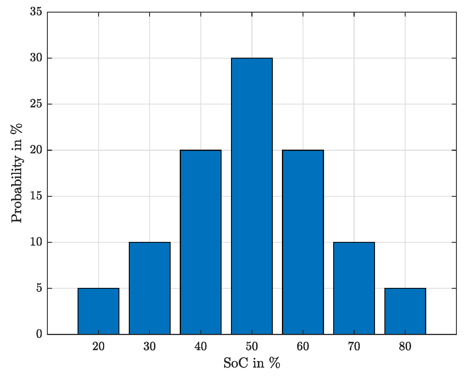
• In the fourth step, the $SoC$s before $SoC$_Start and after $SoC$_End the charging process are determined. These depend on the chosen scenario and are, therefore, explained in detail in Section 6. The necessary charging energy E_Charging is calculated as follows

  $$E_{\mathrm{Charging}}=(SoC{}_{\mathrm{End}}-SoC{}_{\mathrm{Start}})·E_{\mathrm{Cap}}.$$

  (4)
• The duration of the charging process T_Dur is determined as follows:

  $$T_{\mathrm{Dur}}=E_{\mathrm{Charging}}·T_{\mathrm{Char}}.$$

  (5)
• The end-time of the charging process T_End is calculated using the arrival time T_Arr and the duration of the charging process T_Dur.

  $$T_{\mathrm{End}}=T_{\mathrm{Arr}}+T_{\mathrm{Dur}}.$$

  (6)
• In the seventh step, the maximum daily simultaneity factor is determined by generating a charging profile for each EV and by considering T_Arr and T_End of each EV.
• Finally, the charging profile is divided between the different phases following the input data. For each phase, all profiles are added to a common charging profile N_{EV,Profile,PhaseX}. Then, the maximum number of simultaneously charging cars N_{EV,Simul,PhaseX} is reviewed for the grid and each feeder. This number is then divided by the total number of cars N_EV,Total in each grid or feeder to calculate the simultaneity factor of the EV charging process. N_EV,Total corresponds to the number of involved grid customers n as introduced in Section 4.1 and has to be determined depending on the grid limit that has to be verified, as explained in Section 4.2.

  $$s_{\mathrm{EV}}=\frac{N_{\mathrm{EV},\mathrm{Simul},\mathrm{PhaseX}}}{N_{\mathrm{EV},\mathrm{Total}}}.$$

  (7)
  The maximum peak power P_EV,Peak can then be calculated as follows.

  $$P_{\mathrm{EV},\mathrm{Peak}}=s_{\mathrm{EV}}·P_{\mathrm{Char}}·N_{\mathrm{EV},\mathrm{Total}}$$

  (8)

  $$P_{\mathrm{EV},\mathrm{Profile}}=P_{\mathrm{Char}}·N_{\mathrm{EV},\mathrm{Profile}}.$$

  (9)

5.2. Energy Consumption of Households

In addition to the EV charging, the energy consumption of the households was included to calculate the load-flow in the low voltage grids. To determine the simultaneity factor, profiles for the household energy consumption developed with [27] were used. The profiles were generated for a yearly energy consumption of 1000 kWh. For the households in the grid, a yearly energy consumption of 3216 kWh [28] was assumed. Additionally, it was assumed that 1.3 households were connected to each grid connection point [24] and the profiles were scaled accordingly. As the next steps, all profiles for the regarded grid or feeder are added up to calculate the total consumption profile P_{Household,Profile}. Using this profile, the respective peak power can be determined. Due to missing data, a balanced distribution between the different phases was assumed.

5.3. Total Energy Consumption

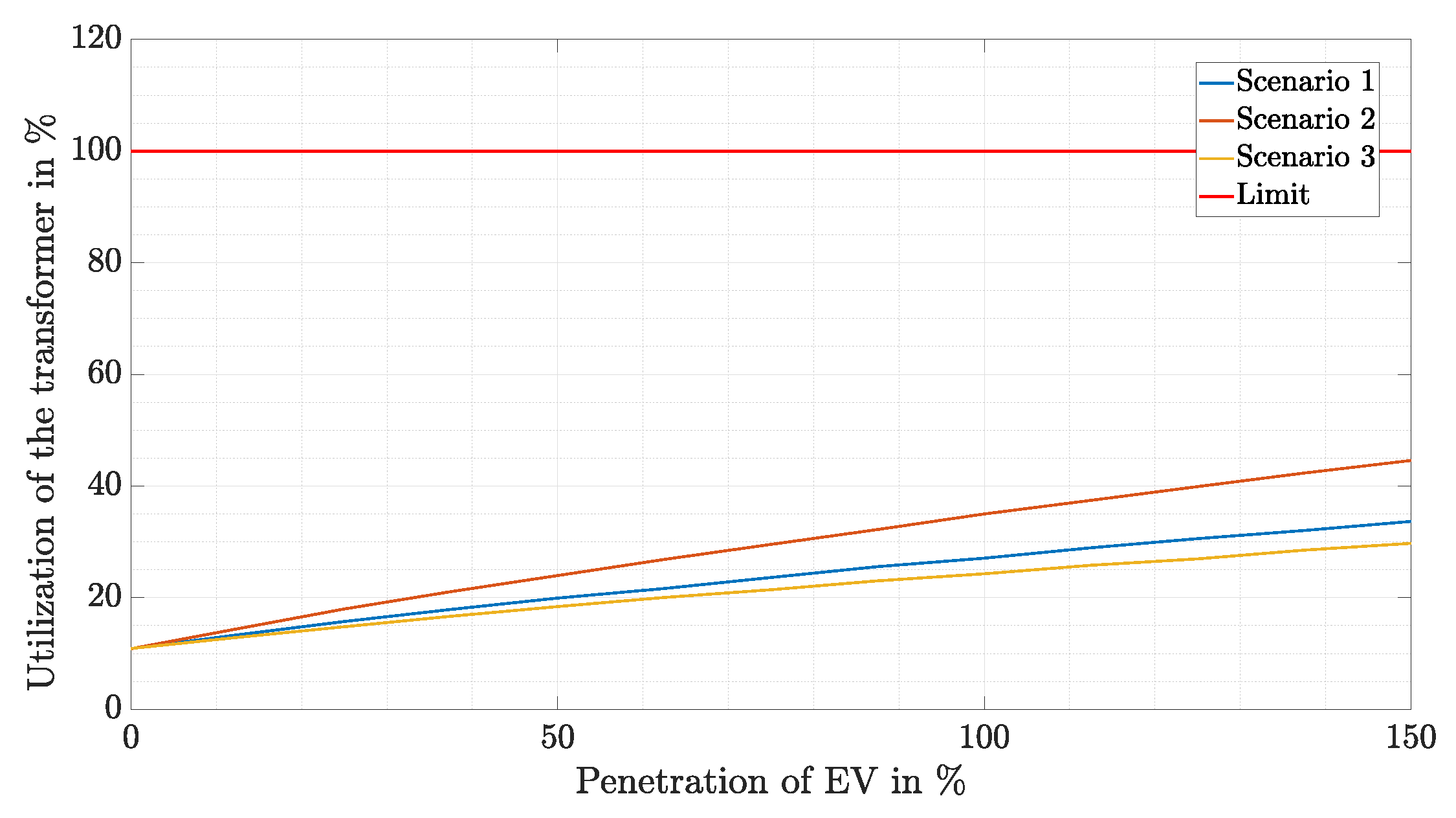
One important aspect to mention is that the times with maximum power for EV charging and the households are different [17]. Hence, it is not is not valid to add the peak power for EV charging and households to calculate the total peak power P_Total,Peak. The related profiles P_{Household,Profile} and P_EV,Profile have to be added to a total profile P_{Total,Profile}. The peak power of this profile is the total peak power P_Total,Peak. As the profile P_EV,Profile depends on the regarded phase, this is also the case for P_Total,Peak.

As we assign input data randomly; P_Total,Peak is subject to statistical deviations. Therefore, we determined P_Total,Peak 100,000 times and used the 99th percentile as the result.

The total peak power P_Total,Peak was then divided by the number of grid connection points in the grid or feeder depending on the criterion to be checked. The result was the power assigned as load to each grid connection point.

6. Scenarios

By means of a comprehensive analysis, all important aspects and parameters concerning the grid impacts of EV should be taken into account. The aim is to define probable future-oriented and crucial scenarios. Therefore, the core parameters market penetration, charging power distribution, battery capacity, charging time, simultaneity factor, $SoC$, and the additional charging possibilities, were considered. In the scope of this contribution, three scenarios, generated from the parameters presented above, were analysed. An overview of the different scenarios and the associated parameters is given in

Table 4. Scenario parameters.

Consideration of
	Simultaneity Factor	$\mathit{SoC}$Start = 0%	$\mathit{SoC}$End = 100%	Driving Distance
Scenario 1	x		x
Scenario 2	x	x	x
Scenario 3	x			x

.

Scenario 1 and Scenario 2 represent the case of “daily recharging.” In these two cases, we attempted to create realistic user profiles. Based on these profiles, all EVs are fully recharged each day ($SoC$_End = 100%) under consideration of the simultaneity factor and the battery capacity. In Scenario 1, the $SoC$ at the beginning of the charging process $SoC$_Start follows the distribution depicted in Figure 8. In comparison, in Scenario 2 the $SoC$_Start is assumed to be 0% which reflects an extreme assumption.

In Scenario 3, it is assumed that all EVs have a daily driving distance of 40 km. Therefore, the required recharge quantity corresponds exactly to the energy quantity consumed for the 40 km. Based on the consumption of the EV and the charging rate, the charging duration was calculated for the daily driving distance average of 40 km.

7. Results

The results in this section have been produced doing load-flow calculations in a simulation framework based on MATPOWER [29]. The LV grids and the associated loads have been modelled as described in Section 2 and Section 5, respectively. The grids were investigated with regard to voltage-related issues and thermal overload.

The following chapter is divided into four parts. In the first part, an exemplary network (Campestral Grid 1) is examined, taking into account the three scenarios (see Section 6). The influence of the individual scenario parameters is considered. In the second part, the focus lies on the regionally different network impacts. To this end, the network effects of one chosen scenario (Scenario 1) are investigated for all network types (campestral, rural, and suburban). The resulting findings are then compared in the third part. The fourth part contains the voltage unbalance in the LV grids.

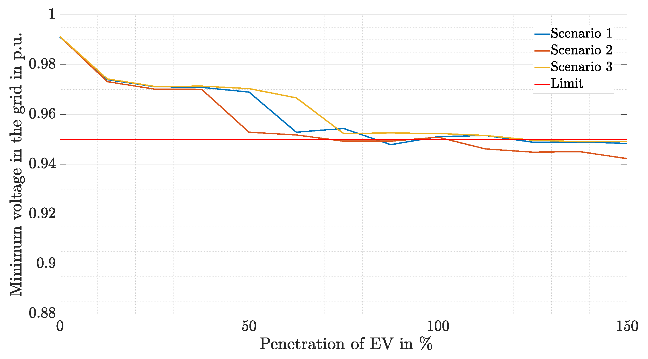
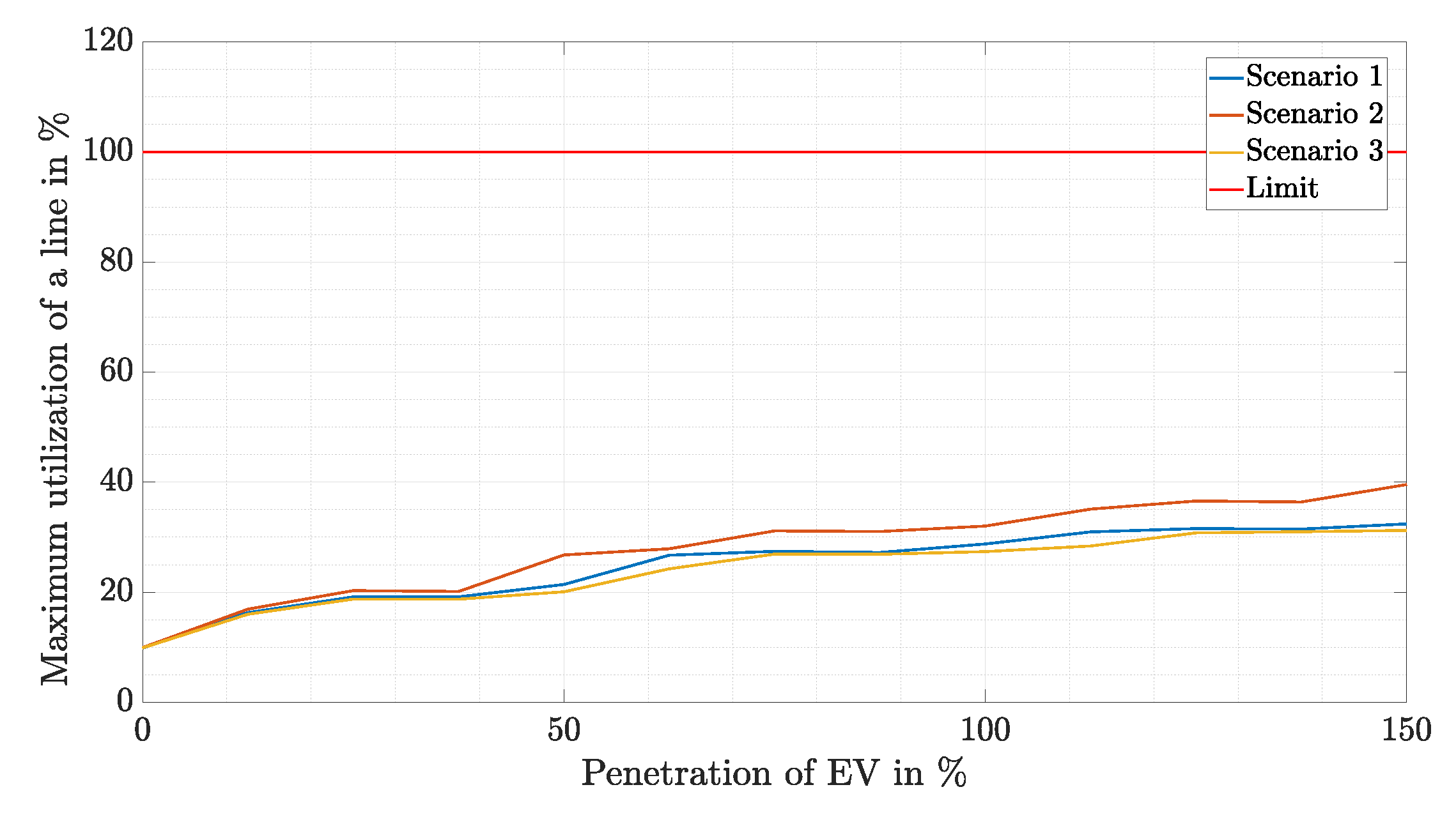
7.1. Impact of the Different Scenarios

In this section, the influence of different scenarios is investigated considering Campestral Grid 1. In Figure 9, the utilisation of the transformer for different penetrations of EVs is shown. In Scenario 2, the utilisation is significantly higher than in the other scenarios. This is reasonable, as the EVs are fully charged in this scenario, so that the charging process duration takes longer than in the other scenarios. Due to the longer charging time, the number of simultaneous charging processes is increased, resulting in a higher total load. As a result, transformer utilisation in Scenario 2 is significantly higher. In Scenario 1 a slightly higher utilisation than in Scenario 3 can be seen. In total, the maximum utilisation for all scenarios is less than 50%. So even for high EV penetration rates, there is no risk of a thermal overload.

In Figure 10, the minimum voltage in the grid is displayed for different penetrations for all three scenarios. Discrete steps in the results are notable. Due to statistical variations in the consumption of the households, the steps are not explicit. The reason lies in the calculation of the minimum grid voltage and the line utilisation. As described in Section 4.2, only the number of households on the relevant feeder is included in these calculations. In Campestral Grid 1, there are two feeders consisting of two respectively six households (see Figure 3). Due to this small number of households, it is not possible to apply thirteen different penetrations. As rounding is used in the calculation, the same number of cars was assumed for different penetrations. Hence, the results are similar for different penetrations and discrete steps occur. The valid minimum voltage limit was exceeded for high penetration rates in all three scenarios.

In Figure 11, the utilisation of the maximally utilised line in the grid is shown for different penetrations. Again, discrete steps can be observed in the results. As for the other equipment, the biggest stress on the line is in Scenario 2, while Scenario 1 and Scenario 3 show similar results. The limit is not exceeded, even for the highest penetrations.

In conclusion, the different scenarios have a significant influence on the voltage-related and thermal utilisation of the equipment. Therefore, the choice of a realistic scenario is decisive for the performance of network analyses. In the following section, only Scenario 1 is considered for the following analysis. This can be explained by the fact that Scenario 3 shows a high similarity with regard to the results and Scenario 2 does not depict reality accurately (user surveys show that the the $SoC$ at the beginning of the charging process is just rarely 0%) and represents therefore an extreme scenario.

In the following subsection the different grid types (campestral, rural, and suburban grids) are investigated.

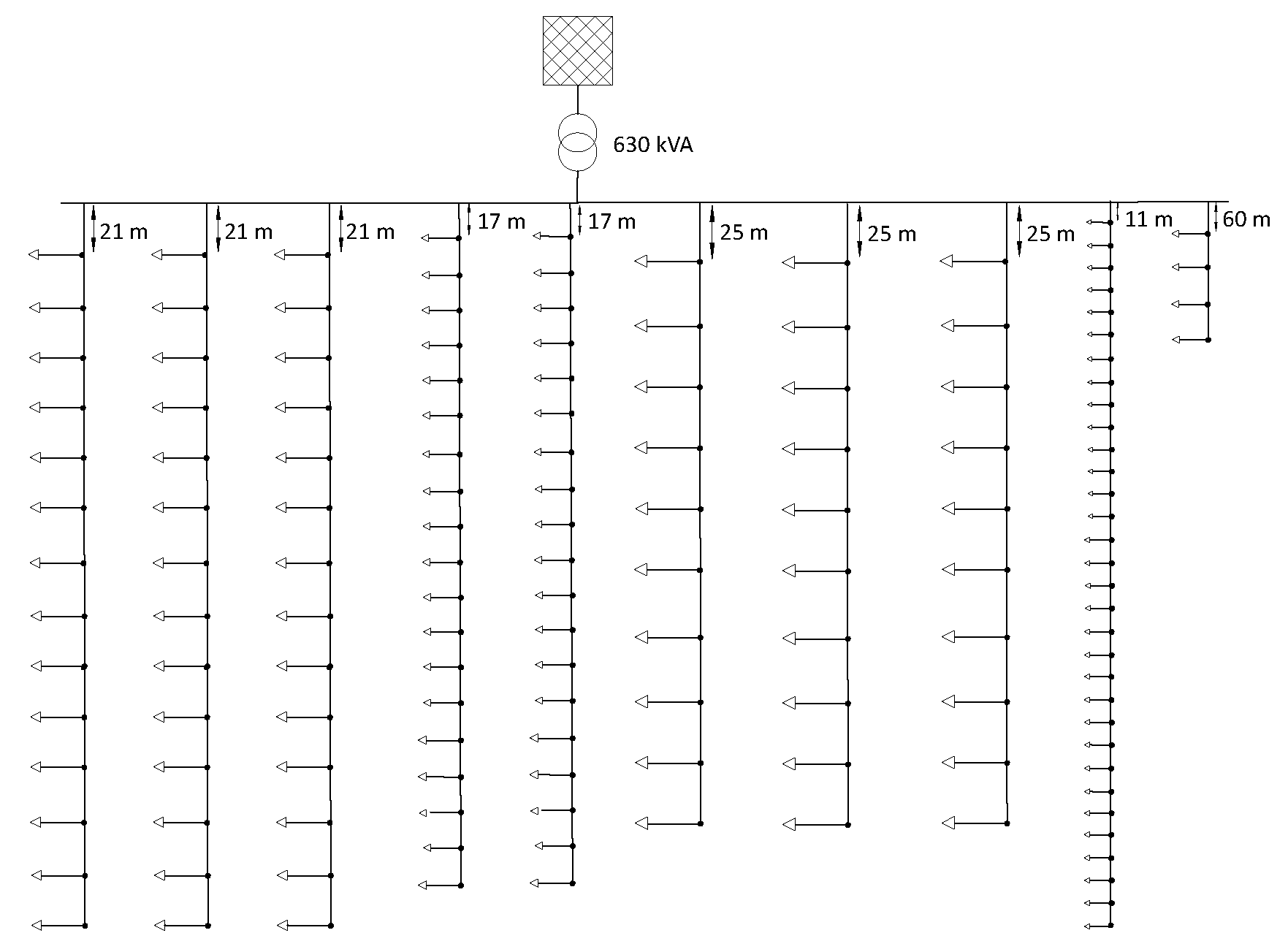
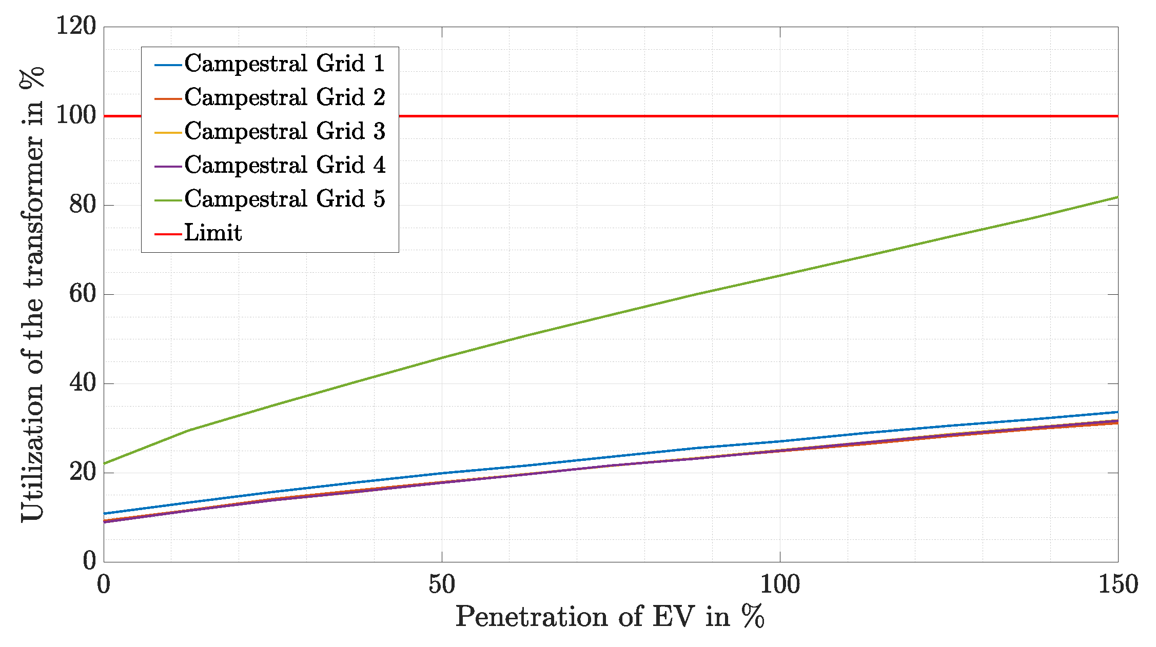
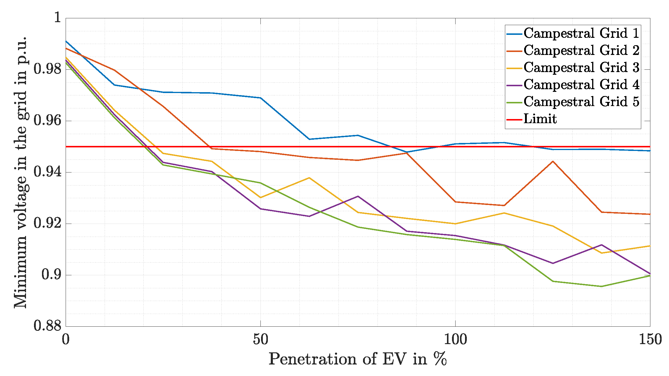
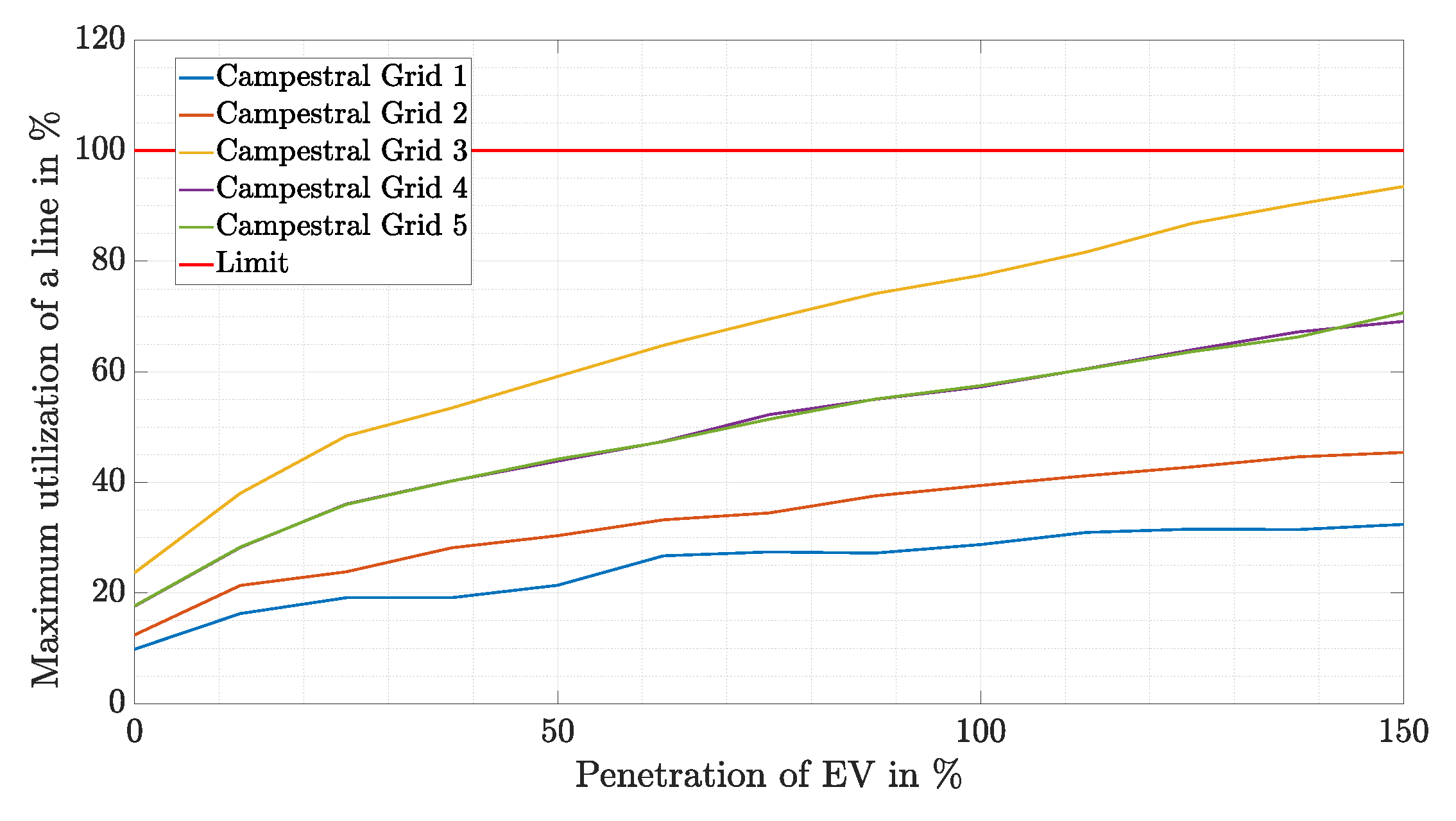
7.2. The Campestral Grid

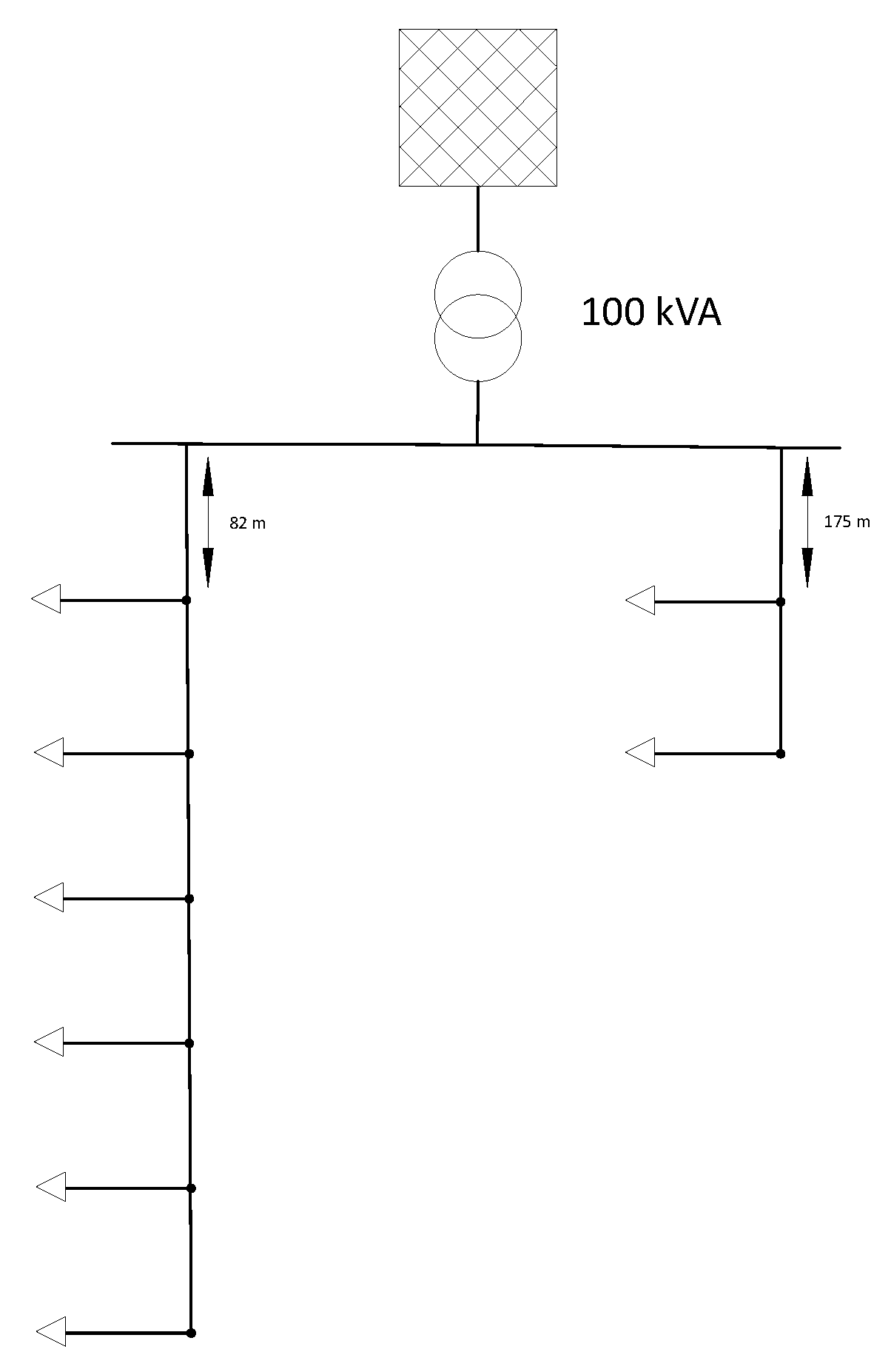
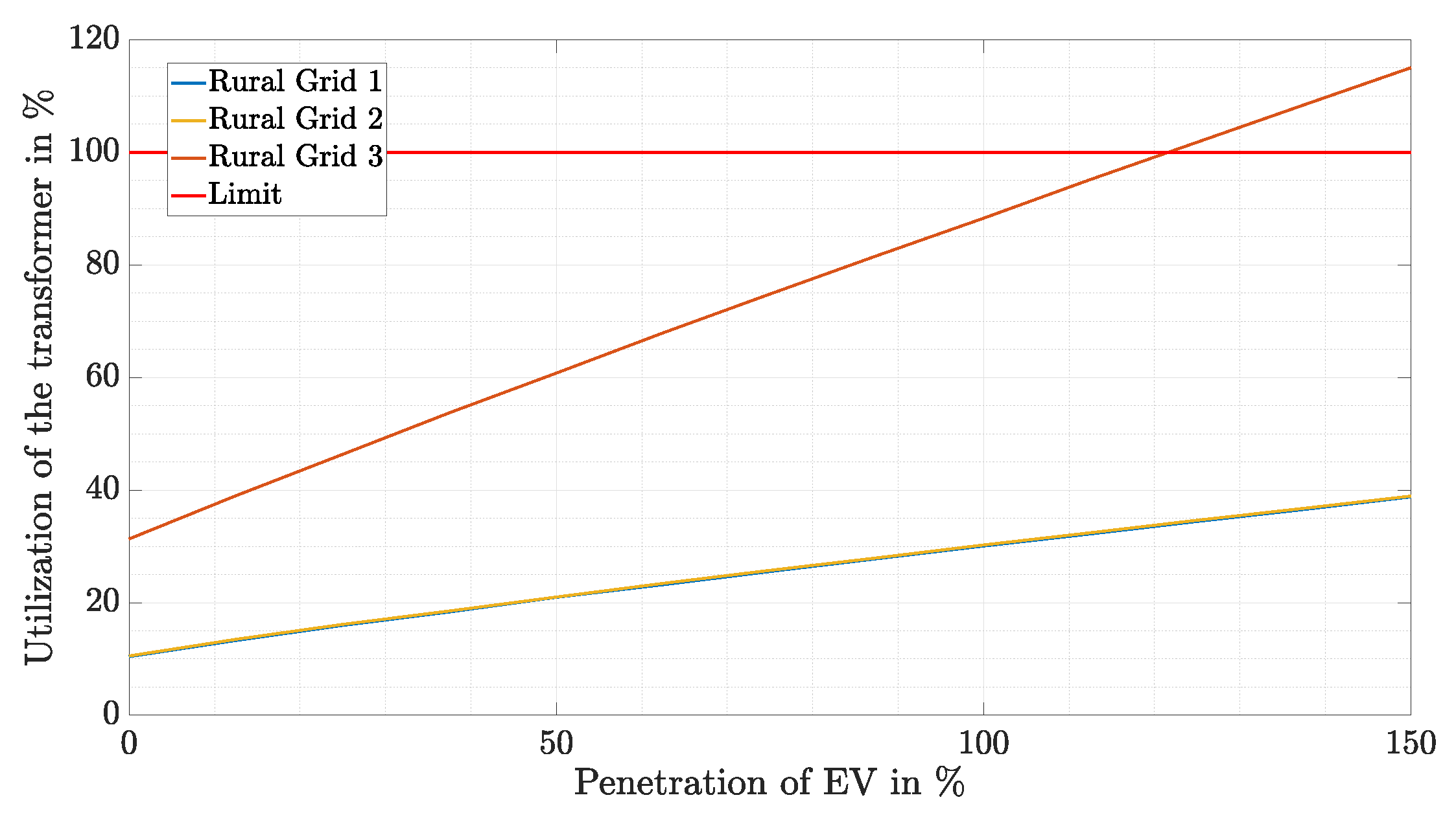
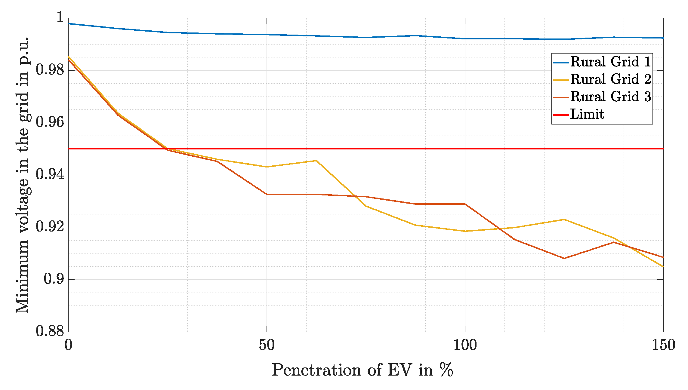
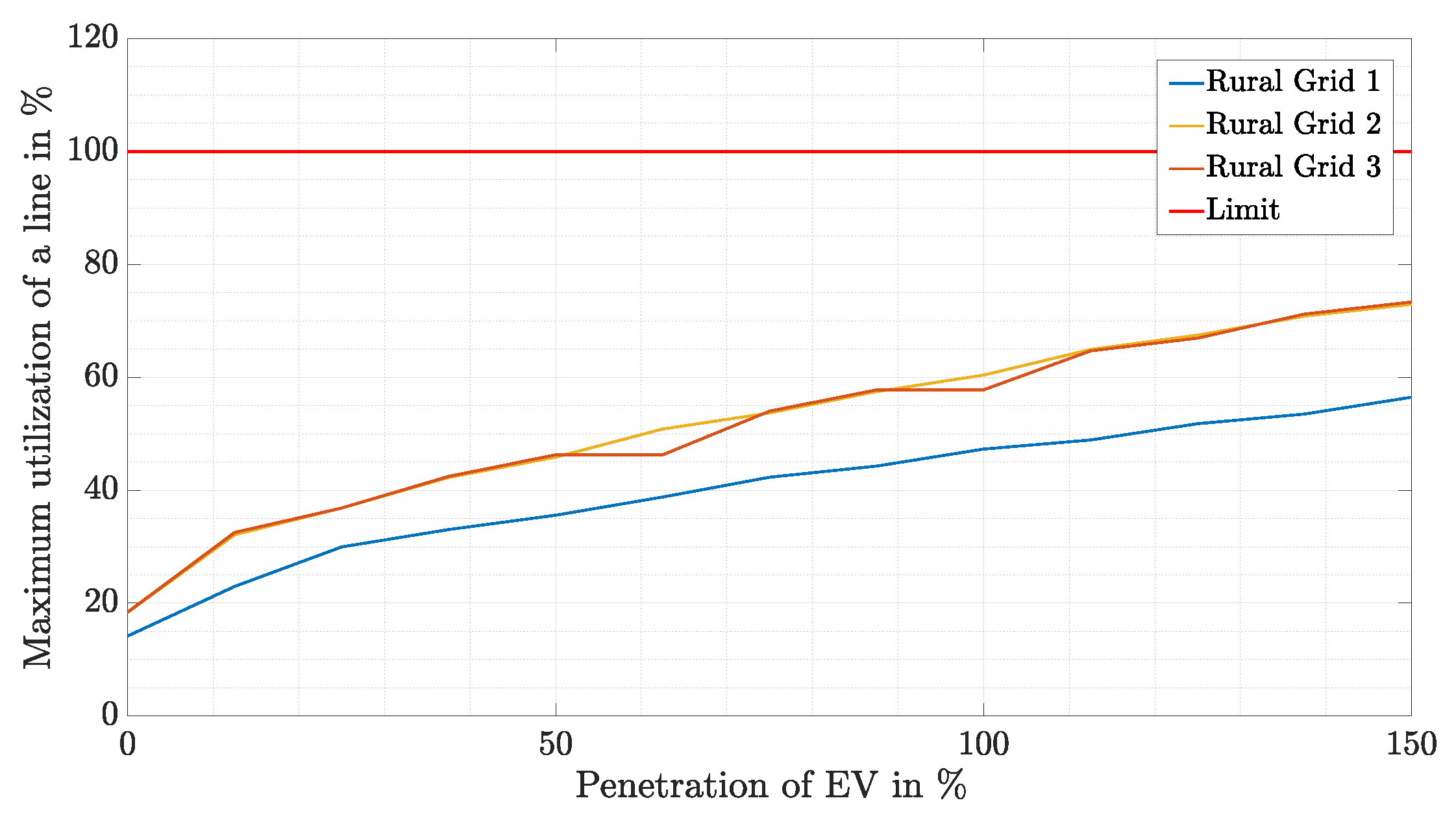
In this section, the results for the different campestral grids are shown and compared. In Figure 12, the utilisation of the transformer is shown. Campestral Grids 1–4 show similar results. This is reasonable, as the ratio between number of households and nominal power of the transformer in these grids is similar. Only the grid structure and the distance between the households is varied see Section 2. In comparison Campestral Grid 5, which is representative for a grid with comparably high transformer utilisation, is characterised by a significantly higher utilisation for the different penetration rates. But even for a penetration of 150% for EVs, the transformer limit is not exceeded.

In Figure 13, the minimum voltage in the grid is depicted. As the feeder length influences the voltage drop in the grid, in Campestral Grids 3–5 the minimum voltages are significantly lower than in Campestral Grid 1 and Campestral Grid 2. Nevertheless, for penetrations higher than 125%, the minimum voltage exceeds the given limit in all grids. As a result, it can be said that voltage drop is a limiting parameter for the integration of EV in campestral grids.

In Figure 14, the maximum utilisation of a line in the regarded grids is shown. Campestral Grid 4 and Campestral Grid 5 show similar results, as the main difference between these grids is the nominal power of the transformer which does not influence the power flow on the cables. Campestral Grid 3 contains the cable with the highest utilisation. This cable has a smaller diameter, and hence a smaller current limit than comparable cables in Campestral Grid 4 and Campestral Grid 5. In comparison to Campestral Grid 1 and Campestral Grid 2, there are additionally more households connected to the feeder with the most utilised line.

Finally, it has to be stated that no line is overloaded for any penetration independent of the grid considered. Comparing the maximum utilisation of transformer and cables, a higher transformer utilisation can be determined; see Figure 12 and Figure 14.

7.3. The Rural Grid

In Figure 15, the utilisation of the transformer is shown for different rural grids. Rural Grid 1 and Rural Grid 2 show similar behaviour, whereas the transformer utilisation in Rural Grid 3 is significantly higher and shows an overload for penetrations of more than 125%. Nevertheless, it should be noted that Rural Grid 3 is characterised by a higher transformer utilisation, even without taking EV into account.

In Figure 16, the minimum voltage in the grid is shown. For Rural Grid 1, only small voltage drops can be observed. The results of Rural Grid 2 and Rural Grid 3 are quite similar as the lengths of the feeders in these grids are similar. While in Grid 1 there occurs no underrun of the minimum voltage, in the latter two the voltage limit is underrun from a penetration of 25%.

The current limits in the lines were not exceeded for any penetration and for any of the rural grids; see Figure 17.

As the number of households per feeder is higher in Rural Grid 2 and Rural Grid 3, the maximum line utilisation is also higher for these grids compared to Rural Grid 1. Grid 2 and Grid 3 show very similar behaviour, since the only difference between the two networks is the power rating of the transformer and number of feeders, which both do not influence the utilisation of the lines.

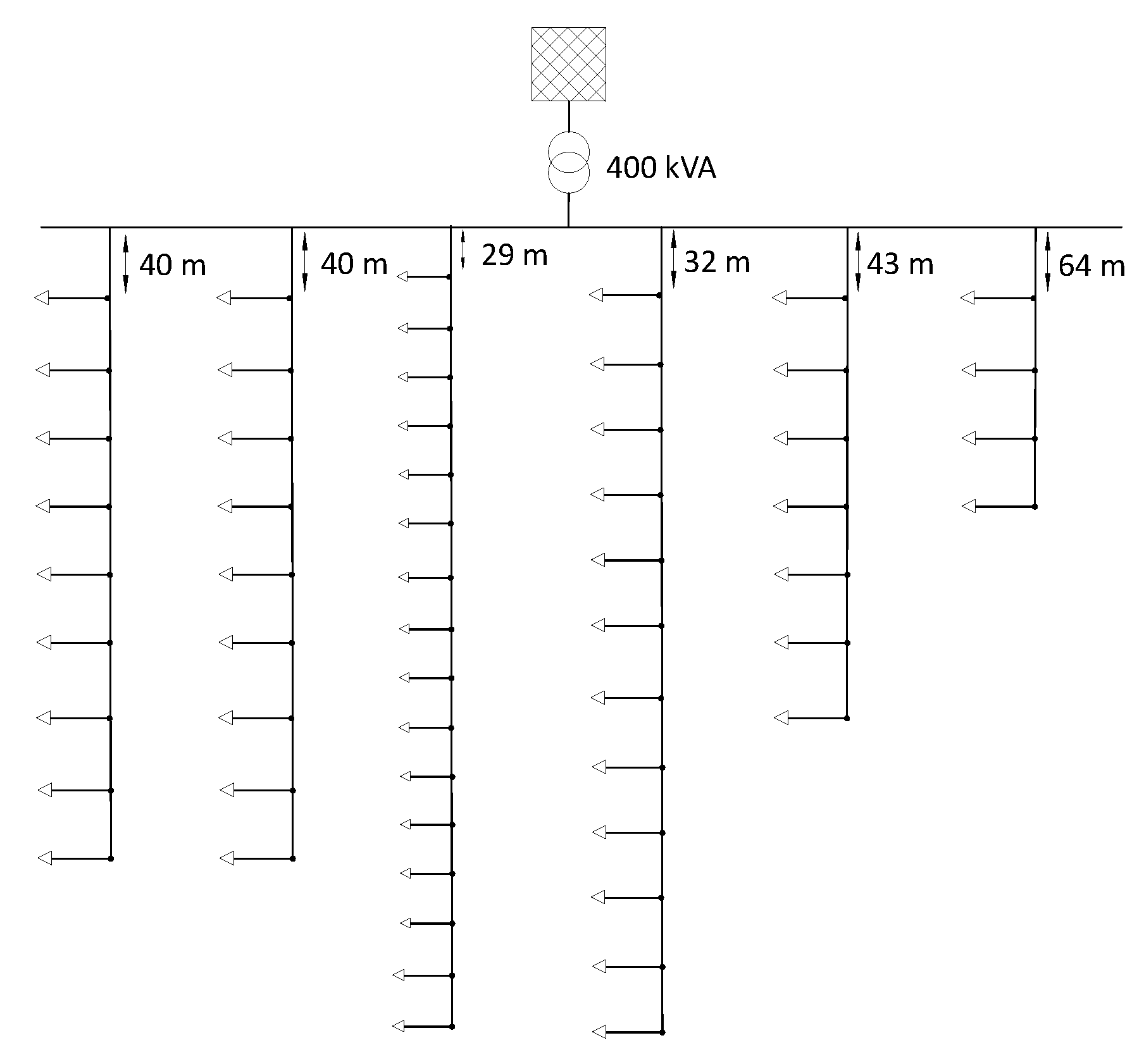
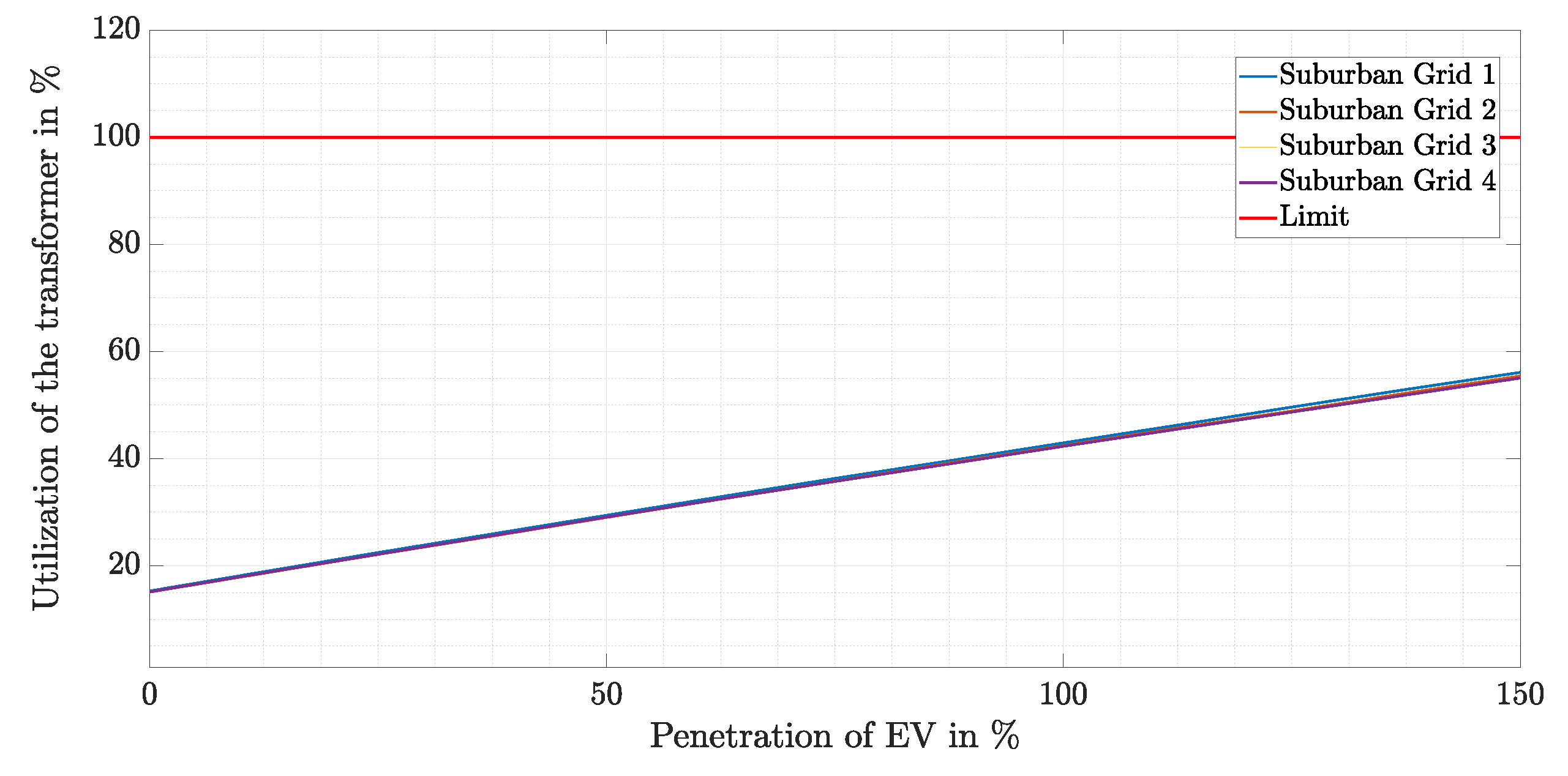
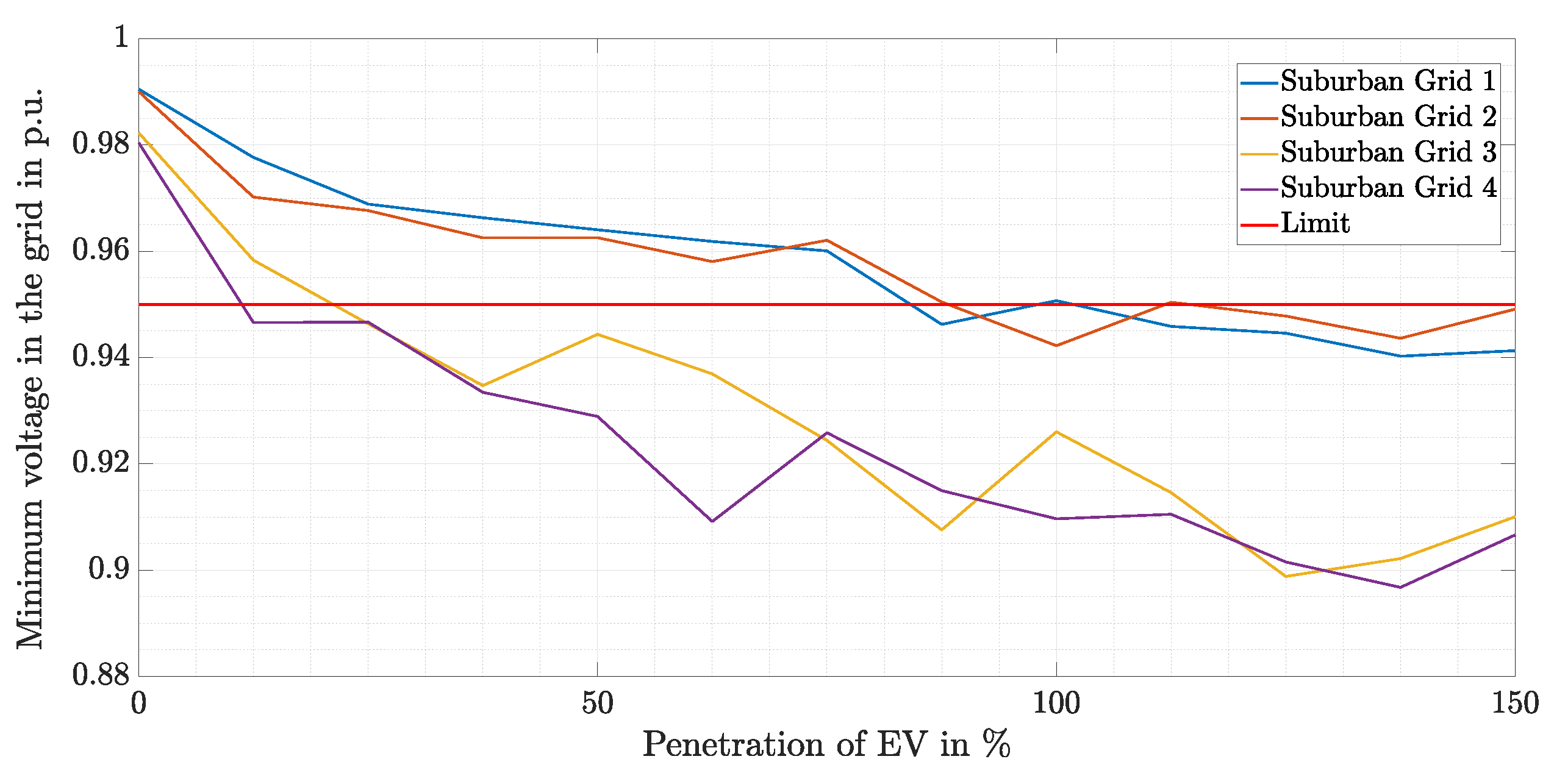
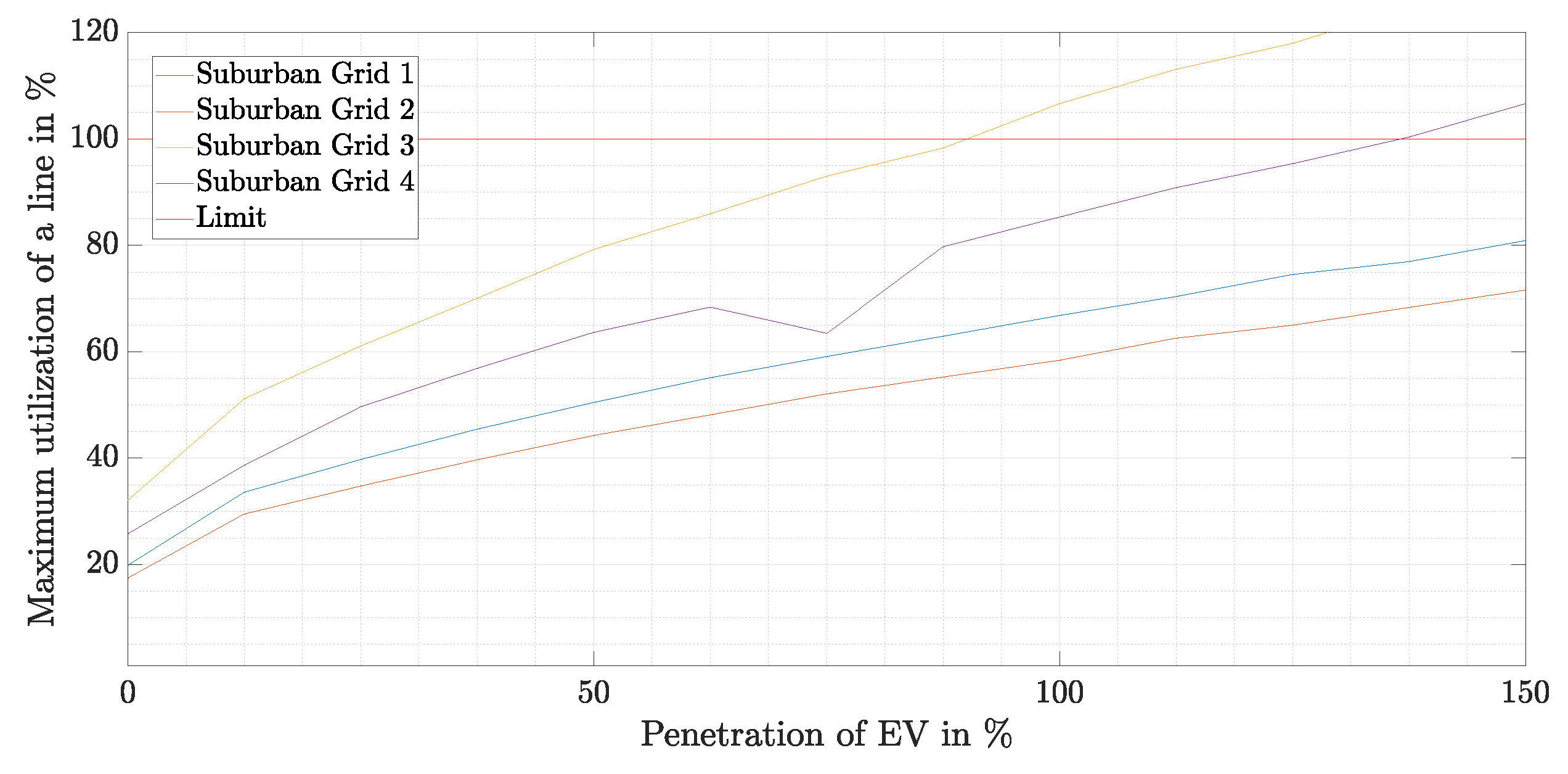
7.4. The Suburban Grid

The suburban grids differ only minimally with regard to the results of transformer utilisation for increasing market penetration. With increasing market penetration, the transformer utilisation also increases due to the additional load. However, the maximum capacity of the transformer is not reached for any of the suburban grids and penetration rate, see Figure 18.

Considering the minimum voltage level in the different suburban grids, an increasing market penetration of EV indicates a voltage drop. Since Suburban Grid 3 and Suburban Grid 4 are characterised by extremely long feeders, the minimum voltage is below the corresponding minimum voltage level of Suburban Grid 1 and Suburban Grid 2.

Since the feeder length has a significant influence on the voltage level, the minimum voltage limit in Suburban Grids 3 and 4 undershot with a penetration of 12.5% and with 25% market penetration, respectively. In Suburban Grids 1 and 2, the limit was only exceeded from penetration rates of 75% and 87.5%, respectively. The corresponding voltage levels for all suburban grids is presented in Figure 19.

Considering the utilisation of the lines as a function of market penetration in Figure 20, it can be seen that the utilisation increases with increasing market penetration.

Since line utilisation is also related to feeder length as more households are connected at longer feeders, a higher utilisation can be observed for Suburban Grid 3 and 4. For Suburban Grid 3, the maximum line capacity is exceeded from a penetration of 87.5%. The lines of Suburban Grid 1 and 2 are not overloaded regardless of market penetration. As already mentioned, in comparison to the utilisation of the transformer, a higher utilisation can be seen for the cables.

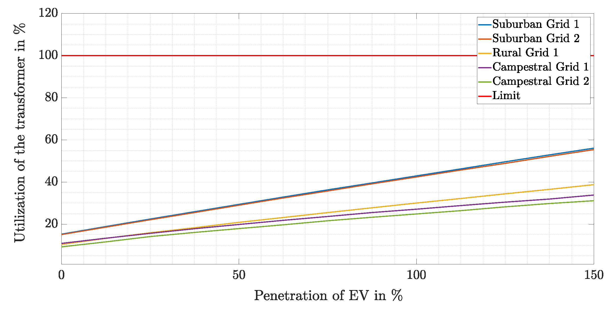
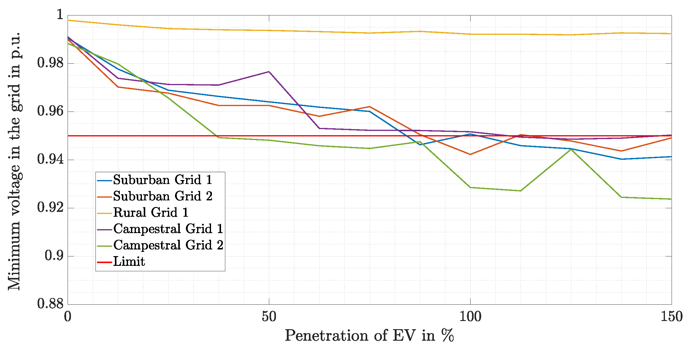
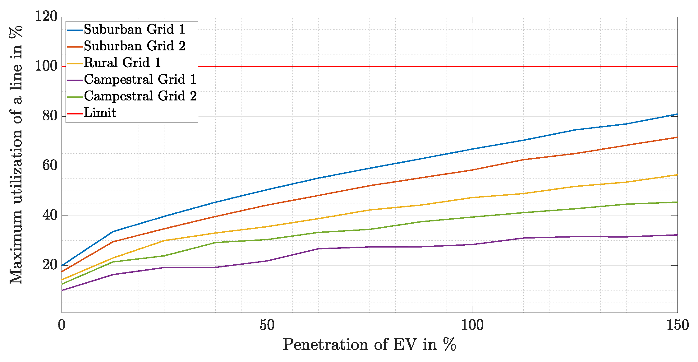
7.5. Comparison of the Different Types of Low Voltage Grids

This section compares the different network types with regard to thermal and voltage overloads. Suburban Grids 1 and 2, Rural Grid 1 and Campestral Grids 1 and 2 are included in the analyses. The transformer utilisation for numerous market penetrations for the different grid types is shown in Figure 21. Since the utilisation of the transformer depends mainly on the connected users, the utilisation is highest in Suburban Grid 1 and 2. In comparison to the campestral grids, the utilisation of the transformer in Rural Grid 1 is higher in general. This can be explained by the corresponding number of connected users in the related grids. However, the thermal capacity of the transformer is not exceeded in any of the grids independent of the market penetration.

The minimum voltage in the networks, is given in Figure 22. With an increasing penetration, the minimum voltage level in all networks decreases. In Rural Grid 1, there are no violations of the minimum voltage level and only minimal voltage drops occur. In Campestral Grid 2, the first violation of the limit occurs at a penetration rate of 37.5%.

From a market penetration of 100%, the lower voltage limit is exceeded in all networks.

The utilisation of the lines in the different grids is shown in Figure 23. The utilisation of a line increases with increasing market penetration. But even here, the lines are not overloaded in any of the grid types.

In connection with the length of the individual cables and the connected users, the suburban grids have the highest load factor and the campestral grids the lowest load factor. The utilisation of the cables is usually higher than the utilisation of the transformer, and can, therefore, be seen as a limiting factor in the grid integration of EVs. In summary, in suburban grids a higher utilisation of transformer and lines can be identified. This rises with an increasing market penetration of EV. The capacity utilisation of rural and campestral grids is generally lower. This can be explained by the higher number of households and the associated higher load in suburban grids. With regard to voltage limits, campestral grids are most likely to risk a violation.

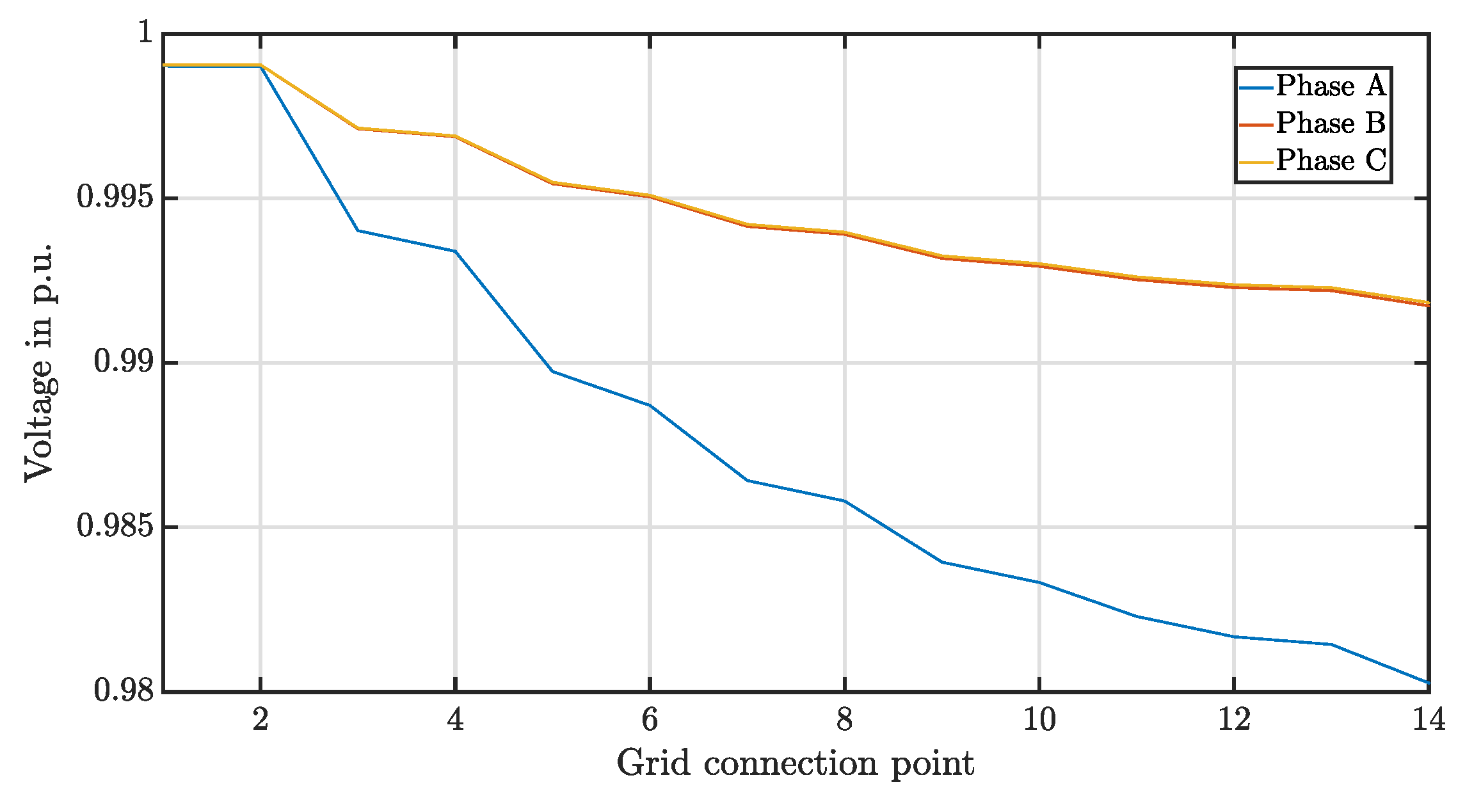
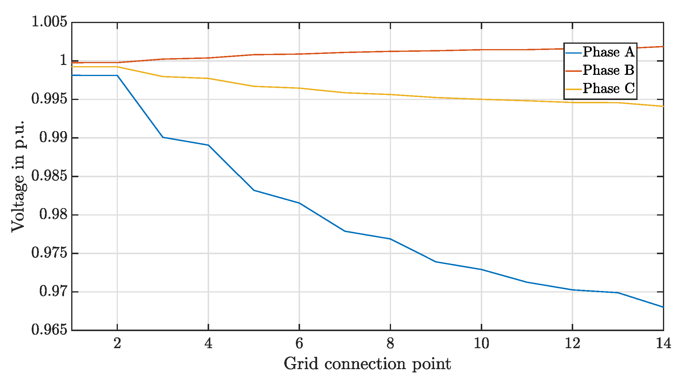
7.6. Voltage Unbalance in the Low Voltage Grids

The voltage unbalance was not mentioned in the previous result sections, as the limit of 2% (see Section 3) was not exceeded in any simulation for this publication. In

Table 5. Maximum voltage unbalance in the regarded low voltage grids.

Grid Name	Voltage Unbalance in %
Campestral Grid 1	0.83
Campestral Grid 2	1.18
Campestral Grid 3	1.33
Campestral Grid 4	1.48
Campestral Grid 5	1.53
Rural Grid 1	0.31
Rural Grid 2	1.34
Rural Grid 3	1.34
Suburban Grid 1	0.82
Suburban Grid 2	0.86
Suburban Grid 3	1.37
Suburban Grid 4	1.4

, the maximum voltage unbalance for different grids is shown. One result is that for grids with longer feeders (e.g., Rural Grid 2 and Rural Grid 3), the voltage unbalance is significantly higher than for grids with shorter feeders (e.g., Rural Grid 1).

To improve the review of the voltage unbalance, it is necessary to take into account a voltage unbalance at the low voltage side of the transformer. In this publication, voltage unbalance is assumed to be 0% at the low voltage side of the transformer. Furthermore, additional unbalanced power flows, which are caused by the households, have to be considered. At the moment, no appropriate data is available to model this more accurately. Taking into account these effects as well would lead to higher voltage unbalances. Consequently, as a result of our simulations we can conclude that EV charging has a strong impact on voltage unbalance in grids with long feeders, but to verify compliance with the given limits, more accurate simulations have to be done in the future.

8. Summary and Outlook

In this paper, twelve low voltage grids that are typical for German agglomerations have been modelled, including the power demand for households and EV charging. For the EV charging, simultaneity factors have been calculated using realistic input data to determine the maximum yearly power demand. The developed models have been used to perform load-flow calculations to determine the impact of the EV charging on the grid operation. Therefore, the compliance with limits given in standards was verified.

As shown in the analysis of the individual networks, voltage stability is the main critical factor in the integration of EVs into the low voltage grids. For high penetrations of EVs, in all grids, the minimum voltage in the grid was close to the limit or even exceeded. The thermal limits were only exceeded for grids with special characteristics and were far below the given limits for most of the grids. Higher utilisation of equipment can be observed for the suburban grids compared to campestral and rural grids.

Previous studies mainly identified the utilisation of transformers as critical factors, especially for suburban grids [8]. In contrast to these studies, unbalanced charging was not neglected in our research. Unbalanced charging causes additional voltage drops; for example, on the neutral wire. This fact explains the discrepancies in previous studies and highlights the significance of unbalanced charging.

In comparison to the scenarios without EVs, a significant impact of EV charging can be seen for all grids. So as an overall result, it can be said that EV charging has a significant impact on low voltage grids. However, the results cannot be generalised due to the individual network topology. For those grids which are jeopardised by EVs, controlled charging (reduced charging rates or postponed charging) may lead to a relaxation of bottlenecks.

These results are highly relevant for grid operators in order to guarantee a high grid reliability. In the future, actions by grid operators are necessary, as grid limits cannot be fulfilled for high penetrations of EVs. Besides grid expansion, the introduction of controlled charging [8] or the installation of battery storage [30] are promising solutions. Due to long planning and approval periods, required investments should be planned with a significant lead time. Especially the voltage levels in the distribution grid might be an Achilles heel for grid stability.

In particular, it is necessary to have trustworthy models of the low voltage grids and information about charging points with the corresponding charging power in the low voltage grids. Then, grid operators will be able to calculate if grid expansion or further actions are necessary. A mandatory information obligation by residents to grid operators on their installation of charging stations would be advantageous for this challenge.

References

1. International Energy Agency (IEA). Global EV Outlook; International Energy Agency (IEA): Paris, France, 2018. [Google Scholar]
2. Clement-Nyns, K.; Haesen, E.; Driesen, J. The impact of charging plug-in hybrid electric vehicles on a residential distribution grid. IEEE Trans. Power Syst. 2009, 25, 371–380. [Google Scholar] [CrossRef] [Green Version]
3. Clement-Nyns, K.; Haesen, E.; Driesen, J. The impacts of vehicle-to-grid on the distribution grid. Electr. Power Syst. Res. 2011, 81, 185–192. [Google Scholar] [CrossRef]
4. Habib, S.; Kamran, M.; Rashid, U. Impact analysis of vehicle-to-grid technology and charging strategies of electric vehicles on distribution networks—A review. J. Power Sources 2015, 277, 205–214. [Google Scholar] [CrossRef]
5. Yong, Y.J.; Ramachandaramrthy, V.K.; Tah, K.M.; Mithulananthan, N. A review on the state-of-the-art technolgies of electric vehicle, its impacts and prospects. Renew. Sustain. Energy Rev. 2015, 49, 365–385. [Google Scholar] [CrossRef]
6. Rolink, J. Modellierung und Systemintegration von Elektrofahrzeugen aus Sicht der Elektrischen Energieversorgung. Ph.D. Thesis, TU Dortmund, Dortmund, Germany, 2013. [Google Scholar]
7. Shareef, H.; Md Islam, M.; Mohamed, A. A review stage-of-the-art charging technologies, placement methodologies, and impacts of electric vehicles. Renew. Sustain. Energy Rev. 2015, 64, 403–420. [Google Scholar] [CrossRef]
8. Jochem, P.; Märtz, A.; Wang, Z. How might the German distribution grid cope with 100% market share of PEV? In Proceedings of the 31th International Electric Vehicle Symposium, EVS31, Kobe, Japan, 30 September–3 October 2018. [Google Scholar]
9. Tie, C.H.; Gan, C.K.; Ibrahim, K.A. The impact of Electric Vehicle Charging on a Residential Low Voltage Distribution Network in Malaysia. In Proceedings of the IEEE Innovative Smart Grid Technologies, Kuala Lumpur, Malaysia, 20–23 May 2014. [Google Scholar]
10. Nobis, P. Entwicklung und Anwendung eines Modells zur Analyse der Netzstabilität in Wohngebieten mit Elektrofahrzeugen, Hausspeichersystemen und PV-Anlagen. Ph.D. Thesis, TU München, Munich, Germany, 2016. [Google Scholar]
11. Babrowski, S.; Heinrichs, H.; Jochem, P.; Fichtner, W. Load shift potential of electric vehicles in Europe. J. Power Sources 2014, 255, 283–293. [Google Scholar] [CrossRef] [Green Version]
12. Held, L.; Märtz, A.; Wirth, J.; Krohn, D.; Zimmerlin, M.; Suriyah, M.R.; Leibfried, T.; Jochem, P.; Fichtner, W. A Comparison of the Influence of Electric Vehicle Charging on Different Types of Low-Voltage Grids. In Proceedings of the 32nd Electric Vehicle Symposium (EVS), Lyon, France, 19–22 May 2019. [Google Scholar]
13. Kerber, G. Aufnahmefähigkeit von Niederspannungsnetzen für die Einspeisung aus Photovoltaikkleinanlagen. Ph.D. Thesis, TU München, Munich, Germany, 2011. [Google Scholar]
14. Held, L.; Uhrig, M.; Suriyah, M.; Leibfried, T.; Junge, E.; Lossau, S.; Konermann, M. Impact of electric vehicle charging on low-voltage grids and the potential of battery storage as temporary equipment during grid reinforcement. In Proceedings of the E-Mobility Integration Symposium, Berlin, Germany, 23 October 2017. [Google Scholar]
15. DIN e.V. Voltage Characteristics of Electricity Supplied by Public Networks; DIN EN 50160/A1:2016-02; DIN e.V.: Berlin, Germany, 2016. [Google Scholar]
16. Märtz, A.; Held, L.; Wirth, J. Simultaneity Factor Tool. Available online: https://doi.org/10.5281/zenodo.3364366 (accessed on 13 August 2019).
17. Märtz, A.; Held, L.; Wirth, J.; Jochem, P.; Fichtner, W.; Suriyah, M.; Leibfried, T. Development of a Tool for the Determination of Simultaneity Factors in PEV Charging Processes. In Proceedings of the E-Mobility Integration Symposium, Dublin, Ireland, 14 October 2019. [Google Scholar]
18. Kraftfahrtbundesamt, Jahresbilanz des Fahrzeugbestandes am 1. January 2019. Available online: https://www.kba.de/DE/Statistik/Fahrzeuge/Bestand/b_jahresbilanz.html (accessed on 3 September 2019).
19. Kraftfahrtbundesamt, Bestand am 1. Januar 2019 nach Marken, Herstellern. Available online: https://www.kba.de/DE/Statistik/Fahrzeuge/Bestand/MarkenHersteller/marken_hersteller_node.html (accessed on 3 September 2019).
20. Statistisches Bundesamt, Current Population. Available online: https://www.destatis.de/EN/Themes/Society-Environment/Population/Current-Population/Tables/census-sex-and-citizenship-2018.html (accessed on 3 September 2019).
21. Kraftfahrtbundesamt, Bestand am 1. Januar 2019 nach Haltern. Available online: https://www.kba.de/DE/Statistik/Fahrzeuge/Bestand/Halter/halter_node.html (accessed on 3 September 2019).
22. Bundesinstitut für Bau-, Stadt-und Raumforschung, Laufende Raumbeobachtung-Raumabgrenzungen. Available online: https://www.bbsr.bund.de/BBSR/DE/Raumbeobachtung/Raumabgrenzungen/deutschland/kreise/Kreistypen2/kreistypen_node.html (accessed on 3 September 2019).
23. Statistisches Bundesamt, Households, by Type of Household. Available online: https://www.destatis.de/EN/Themes/Society-Environment/Population/Households-Families/Tables/lrbev05.html (accessed on 3 September 2019).
24. Diefenbach, N.; Cischinsky, H.; Rodenfels, M.; Clausnitzer, K. Datenbasis Gebäudebestand; Report; IWU: Darmstadt, Germany, 2010. [Google Scholar]
25. Stöckl, G. Integration der Elektromobilität in das Energieversorgungsnetz. Ph.D. Thesis, TU München, Munich, Germany, 2014. [Google Scholar]
26. Figenbaum, E.; Kolbenstvedt, M. Learning from Norwegian Battery Electric and Plug-in Hybrid Vehicle Users; Institute of Transport Economics, Norwegian Centre for Transport Reasearch: Oslo, Norway, 2016. [Google Scholar]
27. Uhrig, M. Lastprofilgenerator zur Modellierung von Wirkleistungsprofilen Privater Haushalte. Available online: http://doi.org/10.5281/zenodo.803261 (accessed on 13 August 2019).
28. Statistisches Bundesamt, Energy Consumption. Available online: https://www.destatis.de/EN/Themes/Society-Environment/Environment/Material-Energy-Flows/Tables/electricity-consumption-households.html (accessed on 12 August 2019).
29. Zimmerman, R.D.; Murillo-Sánchez, C.E.; Thomas, R.J. MATPOWER: Steady-State Operations, Planning and Analysis Tools for Power Systems Research and Education. IEEE Trans. Power Syst. 2011, 26, 12–19. [Google Scholar] [CrossRef] [Green Version]
30. Held, L.; Krämer, H.; Zimmerlin, M.; Suriyah, M.R.; Leibfried, T.; Ratajczak, L.; Lossau, S.; Konermann, M. Dimensioning of battery storage as temporary equipment during grid reinforcement caused by electric vehicles. In Proceedings of the 2018 53rd International Universities Power Engineering Conference (UPEC), Glasgow, UK, 4–7 September 2018. [Google Scholar]
Figure 1. Suburban Grid 1.
Wevj 10 00088 g001
Figure 2. Rural Grid 1.
Wevj 10 00088 g002
Figure 3. Campestral Grid 1.
Wevj 10 00088 g003
Figure 4. Voltage magnitude between the different phases and ground.
Wevj 10 00088 g004
Figure 5. Voltage magnitude between the neutral line and ground.
Wevj 10 00088 g005
Figure 6. Voltage magnitude between the different phases and neutral line.
Wevj 10 00088 g006
Figure 7. Grid customers that have to be included for the calculation of simultaneities for different grid limits.
Wevj 10 00088 g007
Figure 8. S o C distribution at the beginning of the charging process.
Wevj 10 00088 g008
Figure 9. Utilisation of the transformer in Campestral Grid 1 for different penetration rates.
Wevj 10 00088 g009
Figure 10. Minimum voltage in Campestral Grid 1 for different penetration rates.
Wevj 10 00088 g010
Figure 11. Maximum utilisation of a line in Campestral Grid 1 for different penetration rates.
Wevj 10 00088 g011
Figure 12. Utilisation of the transformer for different campestral grids depending on the penetration.
Wevj 10 00088 g012
Figure 13. Minimum voltage in different campestral grids for different penetrations.
Wevj 10 00088 g013
Figure 14. Maximum utilisation of a line for different campestral grids depending on the penetration.
Wevj 10 00088 g014
Figure 15. Utilisation of the transformer for different rural grids depending on the penetration.
Wevj 10 00088 g015
Figure 16. Minimum voltage in different rural grids for different penetrations.
Wevj 10 00088 g016
Figure 17. Maximum utilisation of a line for different rural grids depending on the penetration.
Wevj 10 00088 g017
Figure 18. Utilization of the transformer in different suburban grids depending on the penetration.
Wevj 10 00088 g018
Figure 19. Minimum voltage in different suburban grids for different penetrations.
Wevj 10 00088 g019
Figure 20. Maximum utilisation of a line in different suburban grids depending on the penetration.
Wevj 10 00088 g020
Figure 21. Utilisation of the transformer in different grids depending on the penetration.
Wevj 10 00088 g021
Figure 22. Minimum voltage in different grids for different penetrations.
Wevj 10 00088 g022
Figure 23. Maximum utilisation of a line in different grids depending on the penetration.
Wevj 10 00088 g023