Analysis of Optimal Battery State-of-Charge Trajectory for Blended Regime of Plug-in Hybrid Electric Vehicle

Abstract

Plug-in hybrid electric vehicles (PHEV) typically combine several power sources, which call for the use of optimal control strategy design techniques. The PHEV powertrain efficiency can be improved if the battery is gradually discharged by blending fully electric and hybrid driving modes during the whole trip. Here, the battery state-of-charge (SoC) trajectory profile is of particular importance to achieving near-optimal powertrain operation. In order to reveal optimal patterns of SoC trajectory profiles, numerical optimizations of PHEV control variables based on the dynamic programing (DP) algorithm are conducted in the paper. The obtained optimal SoC trajectories are found to form linear-like profiles of minimum length when expressed with respect to travelled distance. Detailed analyses of the DP results point out that the SoC trajectory length is minimized in order to minimize electric losses, which is then reflected in reduced total fuel consumption. This finding is further justified by analyzing the problem of optimal discharging for the simplified battery-only system and for the powertrain as a whole. The impact of engine specific fuel consumption characteristic on the optimal SoC trajectory profile under simplified driving conditions is analyzed, as well.

1. Introduction

Plug-in hybrid electric vehicles (PHEV) are proven to be a viable mid-term solution towards ultimate fully electric vehicles (EV), as they overcome main deficiencies of EVs such as high prices and short range, while allowing recharging from power grid. PHEVs typically operate in charge depleting (CD) and charge sustaining (CS) regimes, where in the CD regime pure electric driving is active until the battery is discharged to a predefined lower-limit level, while in the CS regime hybrid driving is activated in order to sustain the battery state-of-charge (SoC) [1]. In the case of knowing the trip length in advance, it is possible to discharge the battery more gradually under a blended regime and thus further reduce fuel consumption [2,3,4] (typically from 2% to 5% when compared to the CD/CS regime [2]). The optimal SoC trajectory in the blended regime (expressed with respect to travelled distance) tends to have a nearly-linear minimum-length shape for the zero road grade case [2,3,4], while it can significantly deviate from the linear trend in the presence of varying road grade [2,4], low emission zones [5], and non-uniformly distributed driving patterns during driving cycle [3].

In order to fully utilize PHEV potential in the blended regime, it is crucial to determine near-optimal SoC reference trajectory in advance for a wide range of driving conditions, which should be provided to powertrain control strategy and its SoC controller [2,4,6]. In [7], the SoC reference trajectory is calculated by using prediction of upcoming road grade profiles and average driving speeds. In [8], the road grade preview is employed for proper planning of battery usage during driving, where heuristic rules are used to determine a target SoC prior reaching uphill climbing. A predictive HEV energy management strategy calculating the optimal SoC reference trajectory under uncertainties caused by traffic flow and traffic lights is proposed in [9]. In [3], an energy management strategy with road condition preview is proposed, where the optimal SoC reference trajectory is calculated based on predictions of upcoming driving patterns. In order to further reduce fuel/energy consumption, a model predictive control (MPC)-based approach can be used to perform on-line optimizations of PHEV control variables on receding horizon [10,11,12]. In this approach, it is crucial to feed MPC by accurate predictions of future vehicle velocity profile, which can be obtained by using different deterministic or stochastic methods (e.g., based on recurrent neural network [13]). In [11], a hierarchical control strategy performing combined minimization of energy- and battery aging-related costs in MPC manner is proposed, where battery aging is tackled by iteratively calculating a proper battery depth-of-charge (DoD). However, due to inability to predict vehicle velocity profiles accurately on longer time horizons, these MPC applications typically rely on relatively short time horizon predictions (around 10 seconds [10]), and thus cannot ensure global optimality of SoC trajectory. Therefore, the global SoC reference trajectory is typically prepared separately from MPC, and used repeatedly to provide SoC boundary conditions for MPC optimization.

Since the SoC reference trajectory is important to achieve near-optimal powertrain operation both in non-predictive and predictive, and rule- and optimization-based control strategies, this paper aims to provide comprehensive analysis of optimal SoC trajectory patterns in support of SoC reference trajectory synthesis. The analysis is conducted systematically, starting by analysis of dynamic programming (DP) optimization results obtained for different driving conditions, and proceeding by analysis of optimal discharging patterns for the case of simplified battery-only system and for the powertrain as a whole. A convexity analysis of the relevant powertrain functional dependencies is conducted to explain the observed optimal SoC trajectory patterns, in order to further gain insights into the optimal powertrain operation for different driving conditions.

The main contributions of the paper include: (i) proposing a method of generating optimal SoC trajectories of different length with respect to travelled distance and conducting correlation analyses of obtained results, (ii) clarifying the cause and conditions under which the optimal SoC trajectory has the minimum-length linear pattern, and (iii) analytical proof of optimal SoC trajectory pattern for the simplified scenario of battery-only discharging system.

The paper is organized as follows. Section 2 describes mathematical modelling of PHEV powertrain. The DP-based optimization of PHEV control variables and analysis of the corresponding optimization results are presented in Section 3. Section 4 deals with analysis of the optimal SoC trajectory patterns, by considering the optimal battery discharging under various conditions. Concluding remarks are given in Section 5.

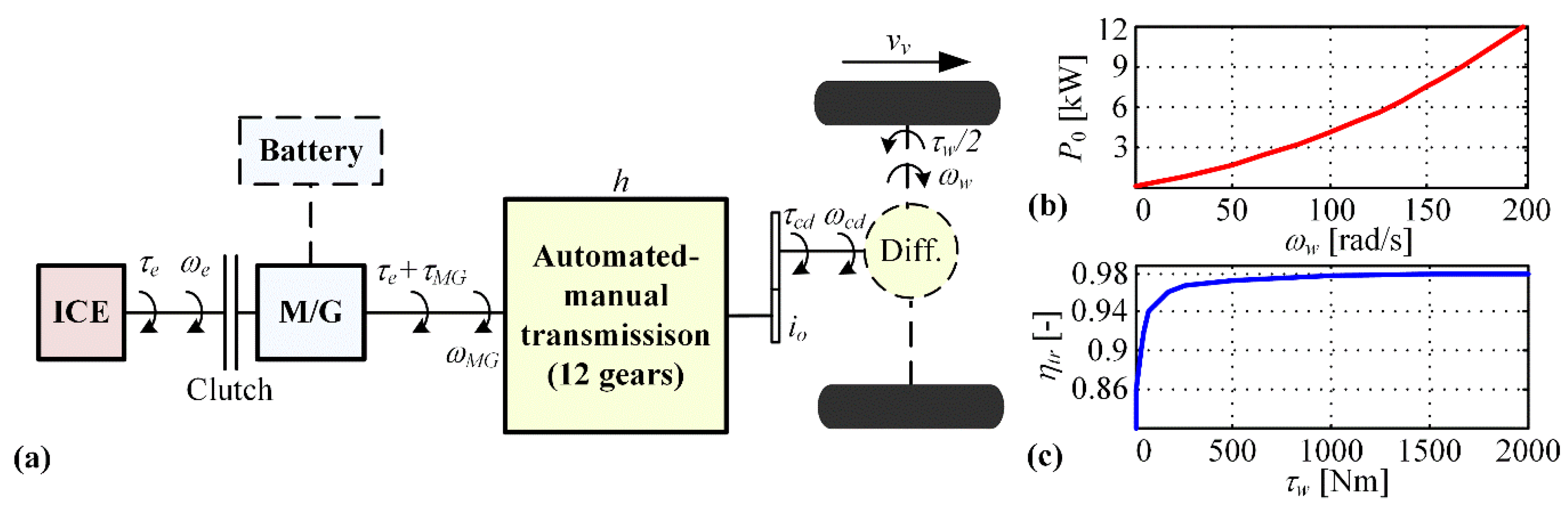
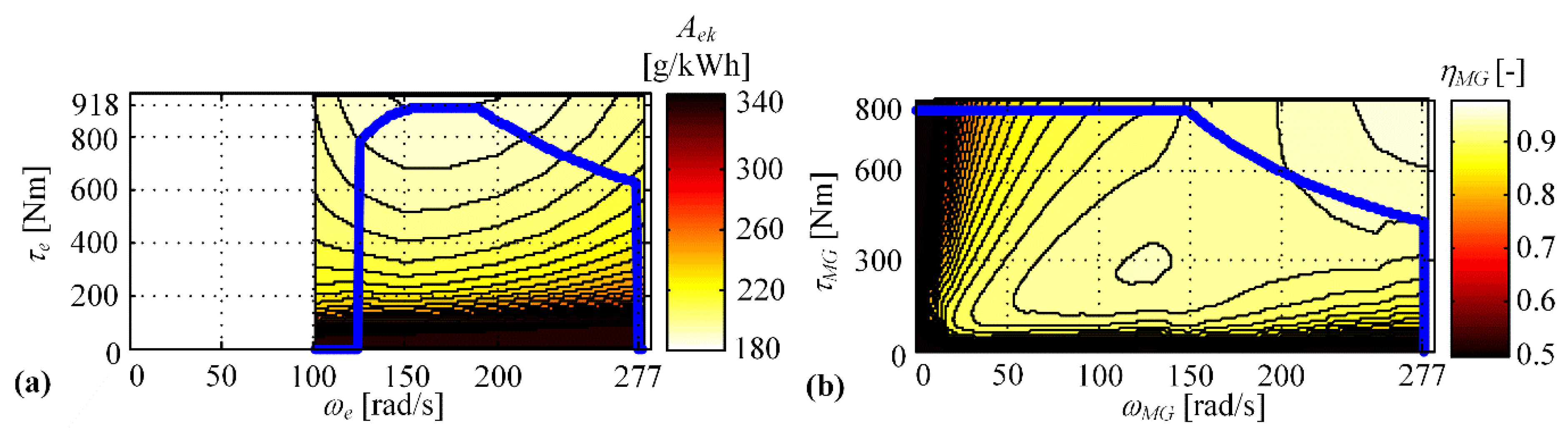
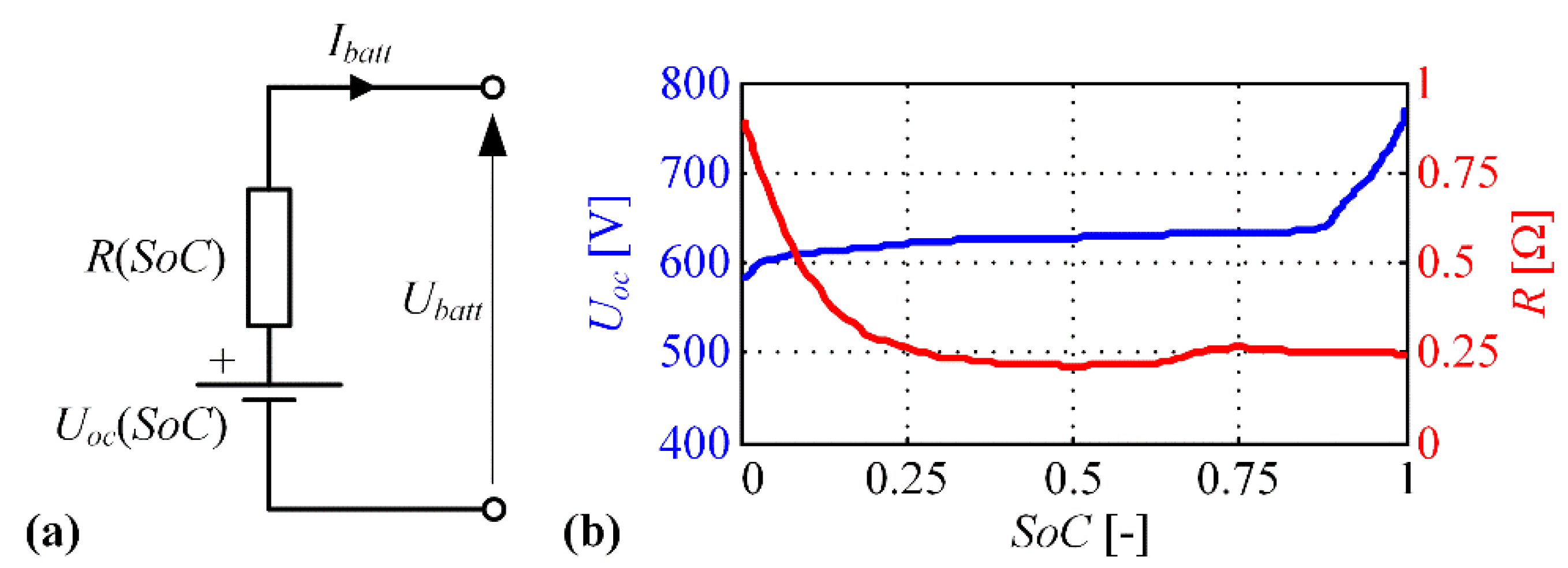
2. Modelling of PHEV Powertrain

Figure 1a illustrates the parallel PHEV configuration of a city bus powertrain considered herein for the purpose of analysis. The powertrain consists of internal combustion engine (ICE), electric machine (M/G), lithium-ion battery and automated manual transmission with 12 gears [14]. When being switched off, the engine can be disconnected from the powertrain by using a clutch, thus enabling electric-only driving. The PHEV powertrain is modelled in the backward-looking manner [15], where the engine and M/G machine rotational speeds are determined by the vehicle velocity $v_v$ and transmission gear ratio $h$ as follows:

$${\omega }_e={\omega }_{MG}=i_{o}h{\omega }_w=i_{o}h\frac{v_v}{r_w},$$

(1)

while the sum of engine and M/G machine torques is obtained from the demanded torque at wheels ${\tau }_w$ and the corresponding drivetrain losses:

$${\tau }_e+{\tau }_{MG}=\frac{{\tau }_{cd}}{i_{o}h}=\frac{\left(\frac{{\tau }_w}{{\eta }_{tr}\left({\tau }_w\right)}+\frac{P_0\left({\omega }_w\right)}{{\omega }_w}\right)}{i_{o}h}.$$

(2)

In Equations (1) and (2), $i_o$ denotes the final drive ratio, ${\omega }_w$ the wheel speed, $r_w$ the effective tire radius, ${\eta }_{tr}$ the transmission efficiency, and $P_0$ the idle-mode power losses (see Figure 1b,c). The total power demand including power losses can then be defined as:

$$P_d={\omega }_w{\tau }_{cd}=\frac{{\omega }_w{\tau }_w}{{\eta }_{tr}\left({\tau }_w\right)}+P_0\left({\omega }_w\right).$$

(3)

The total wheel torque ${\tau }_w$ is calculated according to longitudinal vehicle dynamics equation [14,15]:

$${\tau }_w=r_w\left(\left(M_v+m_{pass}\right)\frac{d{v}_v}{dt}+\underset{F_{roll}}{\underbrace{R_0\left(M_v+m_{pass}\right)g\cos \left({\delta }_r\right)}}+\underset{F_{grade}}{\underbrace{\left(M_v+m_{pass}\right)g\sin \left({\delta }_r\right)}}+\underset{F_{aero}}{\underbrace{{\rho }_{air}{A}_f{C}_d{v}_v^2}}\right),$$

(4)

where $M_v$ and $m_{pass}$ are the empty bus mass and the total mass of passengers, respectively, $R_0$ is the rolling resistance coefficient, ${\rho }_{air}$ is the air density, $A_f$ is the bus frontal surface, $C_d$ is the aerodynamical drag coefficient, ${\delta }_r$ is the road grade, and $g$ is the gravity acceleration (see Appendix A for numerical values of these parameters). The terms $F_{roll}$, $F_{grade}$, $F_{aero}$ are rolling, road grade-related and aerodynamic resistances, respectively.

The engine specific fuel consumption and M/G machine efficiency are modelled by means of 2D maps, while the corresponding maximum torque characteristics are modelled by 1D maps (Figure 2). The specific fuel consumption map ($A_{ek}$), expressed in g/kWh unit, can readily be transformed to the fuel consumption rate map (${\dot{m}}_f$ expressed in g/s unit) by using the following expression:

$${\dot{m}}_f=A_{ek}\left({\tau }_e,{\omega }_e\right)\frac{{\tau }_e{\omega }_e}{3.6·{10}^6}.$$

(5)

The battery is modelled as a charge storage by an equivalent electric circuit (Figure 3a), where the open circuit voltage $U_{oc}$ and internal resistance $R$ are set to be dependent on the battery SoC (Figure 3b; $SoC\in \left[0,1\right]$). Finally, the battery model is represented by the following state equation [16,17]:

$$\dot{SoC}=\frac{\sqrt{U_{oc}^2\left(SoC\right)-4R\left(SoC\right)P_{batt}}-U_{oc}\left(SoC\right)}{2Q_{max}R\left(SoC\right)},$$

(6)

where $Q_{max}$ is the battery charge capacity (here $Q_{max}=$ 30 Ah), while $P_{batt}$ is the battery power which is determined by M/G machine power $P_{MG}$ as:

$$P_{batt}={\eta }_{MG}^{k_{eff}}\underset{P_{MG}}{\underbrace{{\tau }_{MG}{\omega }_{MG}}}.$$

(7)

The variable ${\eta }_{MG}$ is M/G machine efficiency (see Figure 2b), and $k_{eff}$ is equal to one for the case of battery charging ($P_{batt}<0$) and −1 for the case of battery discharging ($P_{batt}>0$).

3. Optimization of PHEV Control Variables

This section deals with DP optimization of PHEV control variables for the blended regime, aimed at finding optimal SoC trajectories for which the total fuel consumption is minimized for different driving cycles and conditions. More details on DP-based optimization of PHEV control variables can be found in [2,18] and references given therein.

3.1. Optimal Problem Formulation

The aim of optimization is to find the values of PHEV control variables in each discrete time step which minimize the cumulative fuel consumption, while satisfying the state- and control variables-related constraints. By introducing the following substitutions for the state variable $SoC$, control variables ${\tau }_e$ and $h,$ and input variables ${\tau }_w$ and ${\omega }_w$:

$$x=SoC,\hspace{1em}u={\left[{\tau }_e h\right]}^T,\hspace{1em}v={\left[{\tau }_w {\omega }_w\right]}^T,$$

(8)

the following discrete-time cost function including cumulative fuel consumption is defined:

$$J={\displaystyle \sum }_{k=1}^{N}F\left(x_k,u_k,v_k,k\right),$$

(9)

$$\begin{array}{cc}\hfill F\left(x_k,u_k,v_k,k\right)=& {\dot{m}}_{f,k}\mathsf{\Delta }T+K_g\left\{H^{-}\left(x_k-So{C}_{min}\right)+H^{-}\left(So{C}_{max}-x_k\right)\right\}\hfill \\ & +K_g\left\{H^{-}\left(P_{batt}^{max}-P_{batt,k}\right)+H^{-}\left(P_{batt,k}-P_{batt}^{min}\right)\right\}\hfill \\ & +K_g\left\{H^{-}\left({\tau }_{e,k}-{\tau }_e^{min}\right)+H^{-}\left({\tau }_e^{max}-{\tau }_{e,k}\right)\right\}\hfill \\ & +K_g\left\{H^{-}\left({\omega }_{e,k}-{\omega }_e^{idle}\right)+H^{-}\left({\omega }_e^{max}-{\omega }_{e,k}\right)\right\}\hfill \\ & +K_g\left\{H^{-}\left({\tau }_{MG,k}-{\tau }_{MG}^{min}\right)+H^{-}\left({\tau }_{MG}^{max}-{\tau }_{MG,k}\right)\right\}\hfill \\ & +K_g\left\{H^{-}\left({\omega }_{MG,k}-{\omega }_{MG}^{idle}\right)+H^{-}\left({\omega }_{MG}^{max}-{\omega }_{MG,k}\right)\right\},\hfill \end{array}$$

(10)

where $k$ denotes the discrete time step, $N$ the total number of discrete time steps, and $\mathsf{\Delta }T$ the discretization time step. Apart from the fuel consumption within each discrete time step ${\dot{m}}_{f,k}\mathsf{\Delta }T$, additional terms are aimed to penalize violation of different constraints. The function $H^{-}$(.) represents the inverted Heaviside function which is equal to 1 when its argument is negative, while otherwise it is equal to 0. The factor $K_g$ is weighting factor which is set to a relatively large value (here $K_g={10}^{12}$) in order to avoid constraints violation. The state equation given by Equation (6) is discretized in time in order to take the following discrete-time form:

$$x_{k+1}=f\left(x_k,u_k,v_k,k\right),\hspace{1em}k=0,1,\dots ,N-1.$$

(11)

The values of initial state variable at $k=0$ and final state variable at $k=N$ are defined as:

$$x_0=So{C}_i,\hspace{1em}{x}_f=So{C}_f.$$

(12)

An additional term $J_f$ penalizing the deviation of the final SoC from the target value $So{C}_f$ is added to the cost function (9) and the control variables optimization problem as:

$$\underset{u_k}{\min }\left(J_f+{\displaystyle \sum }_{k=1}^{N}F\left(x_k,u_k,v_k,k\right)\right),$$

(13)

$$J_f=K_f{\left(So{C}_f-x_N\right)}^2=K_f{\left(So{C}_f-f\left(x_{N-1},u_{N-1},v_{N-1}\right)\right)}^2,$$

(14)

where $K_f$ denotes a weighting factor (here $K_f={10}^6$).

The above-formulated optimization problem is solved by using a dynamic programming (DP), which provides globally optimal results for given discretization resolution of the state and control variables [19] (set as a trade-off between computational efficiency and the optimization accuracy [20]). Numerical values of DP optimization parameters are listed in Appendix A.

3.2. Optimisation Results

DP optimizations of PHEV control variables are conducted for the blended regime and driving cycles shown in Figure 4. The driving cycle denoted by DUB, including the time profiles of vehicle velocity $v_v$, road grade ${\delta }_r$, and passengers mass $m_{pass}$, has been recorded on a real bus operating on a regular bus route in the city of Dubrovnik. Apart from the varying road grade shown in Figure 4b (w/grade), the DUB velocity time profile is also considered for zero road grade (w/o grade). The heavy-duty UDDS driving cycle (HDUDDS) is a certification driving cycle, for which the road grade is zero and empty bus is assumed (m_pass = 0). The DUB driving cycle is repeated three times and HDUDDS two times, in order to provide battery discharging to the minimum allowable SoC level (set here to 30%) in the blended regime under the given driving conditions.

The obtained optimal SoC trajectories (denoted in blue in Figure 5) closely follow the linear profile (red color lines), when they are expressed with respect to travelled distance. Among all possible SoC trajectories spanning between the initial and final SoC values, the linear-like profile has the minimum length. The linear trend is somewhat deteriorated in the case of varying road grade (Figure 5a), where low frequency oscillations appear in the SoC trajectory. These oscillations are caused by battery recharging during regenerative braking on negative road grade segments. Similarity between the optimized and minimum-length (linear) SoC trajectory profiles is quantified by giving values of correlation index K in Figure 5 (calculated by using Matlab function corrcoef(.)), which approaches to the almost ideal value of 1 in the case of zero road grades, and to somewhat lower but still very high value in the case of varying road grades.

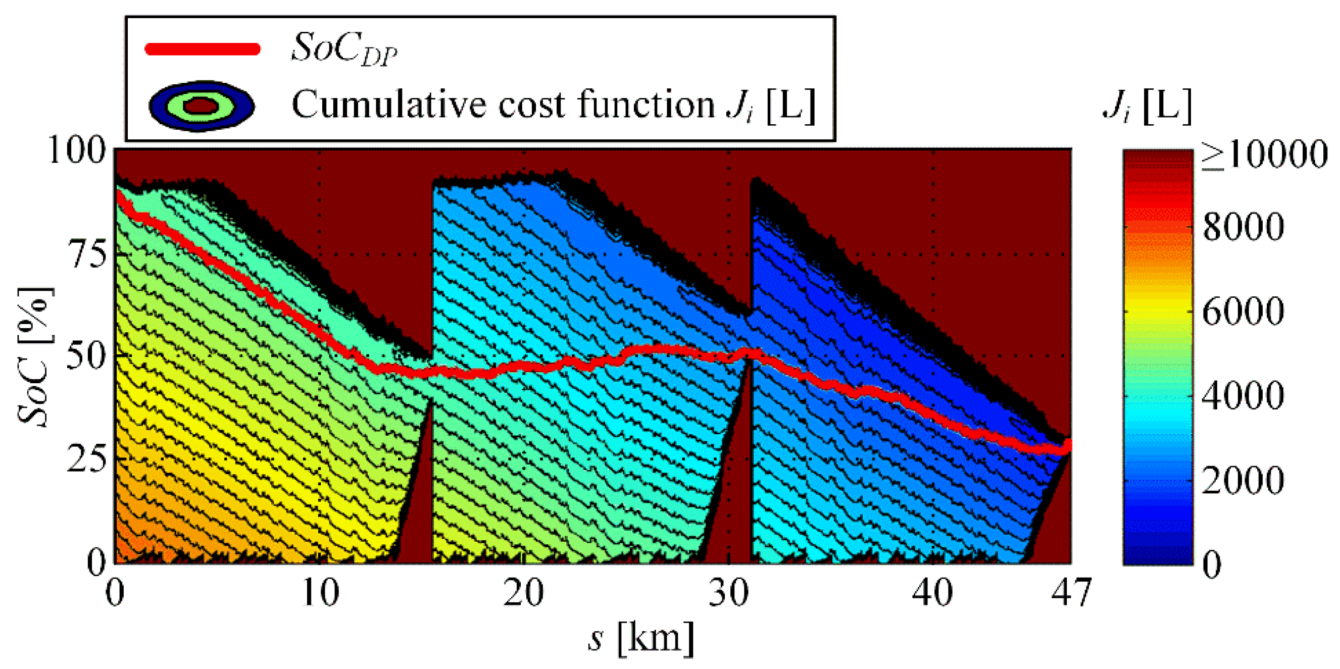
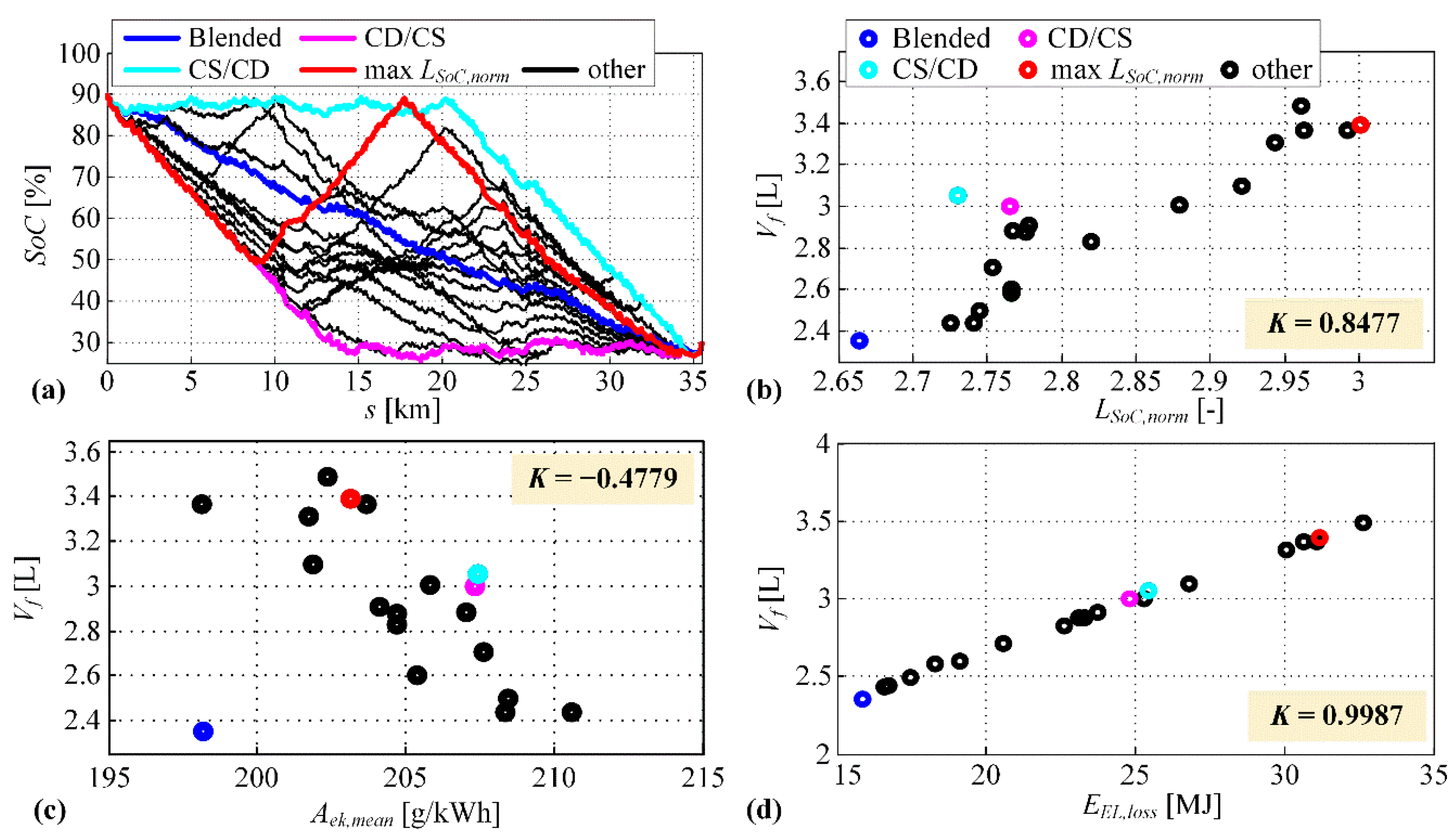
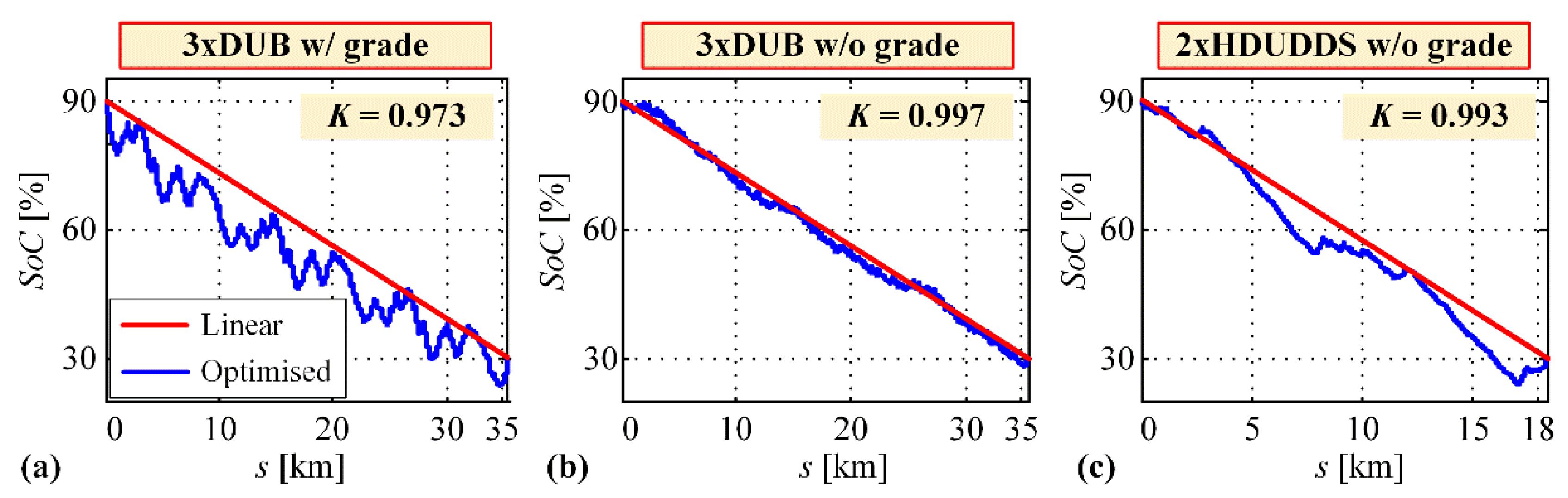
3.3. Generating and Analyzing Optimal SoC Trajectories of Different Length

Based on the results presented in Figure 5 it can be hypothesized that the optimality is closely related to the SoC trajectory length, i.e., that the minimum-length SoC trajectory is optimal. In order to test this hypothesis, the optimal SoC trajectories of different length are generated by adding the following additional SoC constraints to the cumulative cost function (9):

$$J_{SoC,add}={\displaystyle \sum }_j{K}_{SoC,j}{\left(So{C}_{constr,j}-x_j\right)}^2={\displaystyle \sum }_j{K}_{SoC,j}{\left(So{C}_{constr,j}-f\left(x_{j-1},u_{j-1},v_{j-1}\right)\right)}^2,\hspace{1em}j\in C_a.$$

(15)

These constraints penalize the deviation of SoC from several prescribed values $So{C}_{constr,j}$ defined for jth discrete time step, where $C_a$ represents the set of these discrete time steps. Although these SoC constraints are already defined as soft constraints, additional flexibility for optimization is introduced by adding a dead zone of 0.05 (i.e., 5%) around the target values $So{C}_{constr,j}$. This is realized by varying weighting factor $K_{SoC,j}$, which takes the value 0 if $\left|So{C}_{constr,j}-x_j\right|<0.05$, while, otherwise, it takes the value of 5·10⁵. The effect of extending the DP optimization with two additional SoC constraints is illustrated in Figure 6, where the optimal SoC trajectory $So{C}_{DP}$ and the cumulative cost function $J_i$ are shown with respect to travelled distance. The optimal cumulative cost function $J_i$ in the discrete time step $i$ can be calculated as:

$$J_i=\underset{u_k}{\min }\left(J_f+\underset{J_{SoC,add}}{\underbrace{{\displaystyle \sum }_{j\ge i}{K}_{SoC,j}{\left(So{C}_{constr,j}-x_j\right)}^2}}+{\displaystyle \sum }_{k=i}^{N}F\left(x_k,u_k,v_k,k\right)\right),$$

(16)

and it represents the minimal cumulative cost which can be obtained under the imposed constraints, when starting in the considered current SoC and finishing at the final target SoC ($So{C}_f$ = 30%). Extremely large values of $J_i$ ($J_i$ > 10,000) correspond to the SoC values and discrete time steps i for which the final (14) and additional SoC constraints (15) cannot be satisfied under the considered driving conditions. It can be observed that additional SoC constraints cause the cumulative cost function to take relatively low values only in the narrow SoC range of ±5% (corresponding to dead-zone width) in the corresponding time instants. Consequently, the optimal SoC trajectory is forced to pass through these narrow SoC ranges, thus achieving the SoC trajectory of different length when compared to the optimal SoC trajectory obtained when no additional SoC constraints are included.

Apart from the total fuel consumption $V_f$, the total electric energy losses $E_{EL,loss}$ consisting of battery losses $E_{batt,loss}$ and M/G machine losses $E_{M/G,loss}$ are also considered in this analysis:

$$E_{EL,loss}=E_{batt,loss}+E_{M/G,loss }.$$

(17)

The battery losses are dissipated as a heat on its internal resistance $R$ and have quadratic dependence with respect to the battery current $I_{batt}$ (i.e., ${\displaystyle \int }{I}_{batt}{}^{2}Rdt$), while the M/G machine losses depend on the efficiency ${\eta }_{MG}$ (see Figure 2b).

The normalized SoC trajectory length is calculated as:

$$L_{SoC,norm}={\displaystyle \sum }_{k=1}^N\sqrt{\mathsf{\Delta }So{C}_k^2+{\left(\frac{\mathsf{\Delta }{s}_k}{s_f}\right)}^2},$$

(18)

where $\mathsf{\Delta }So{C}_k$ and $\mathsf{\Delta }{s}_k$ represent the difference of SoC and travelled distance between two consecutive time steps (i.e., $\mathsf{\Delta }So{C}_k=So{C}_k-So{C}_{k-1}$, $\mathsf{\Delta }{s}_k=s_k-s_{k-1}$), respectively, while $s_f$ denotes the total travelled distance. Here, only $\mathsf{\Delta }{s}_k$ is normalized with respect to the total travelled distance $s_f$, because the $\mathsf{\Delta }So{C}_k$ already lies in the interval [0,1] by definition and its cumulative sum ${\sum }_k\mathsf{\Delta }So{C}_k$ closely approaches value 1 as ${{\displaystyle \sum }}_k\mathsf{\Delta }{s}_k/s_f=1$.

Figure 7a shows numerous SoC trajectories obtained by DP optimizations for different randomly generated SoC constraints (see Equation (15)) and the case of 3 x DUB with a zero road grade. Some characteristic optimal SoC trajectories are outlined: Blended which corresponds to the case when no additional SoC constraints are included into DP optimization (cf. Figure 5b), CD/CS where the battery is first depleted in pure electric driving and then sustained by means of hybrid driving, CS/CD where the battery discharging is maximally postponed, and $max{L}_{SoC,norm}$ which has the maximum length among all generated SoC trajectories. Note that CD/CS SoC trajectory reveals the all-electric range for the particular driving cycle to be around 15 km. Figure 7b–d show the total fuel consumption $V_f$ with respect to different metrics, where each point corresponds to one optimal SoC trajectory from Figure 7a.

Figure 7b indicates a very high correlation of the total fuel consumption $V_f$ with respect to the normalized SoC trajectory length $L_{SoC,norm}$ (i.e., larger $V_f$ corresponds to larger $L_{SoC,norm}$). Since all SoC trajectories end up in the same value ($So{C}_f$ = 0.3), the observed variations in the fuel consumption for different SoC trajectories may be caused by: (i) different distribution of operating points in the engine specific fuel consumption map, and (ii) different total electric losses calculated by Equation (17). In order to understand these causes better, the total fuel consumptions $V_f$ are shown with respect to the engine mean specific fuel consumptions $A_{ek,mean}$ (Figure 7c), and with respect to the total electric losses $E_{EL,loss}$ (Figure 7d). The results shown in Figure 7c reveal that the cause (i) may be discarded since the larger total fuel consumption often corresponds to even lower mean specific fuel consumption (note negative correlation). On the other hand, very high positive correlation of the total fuel consumption with respect to total electric losses can be observed in Figure 7d, thus revealing that the electric losses are responsible for the fuel consumption variations when SoC trajectories of different length are generated. For most of the SoC trajectories, the engine efficiency reflected through the mean specific fuel consumption is somewhat sacrificed, in order to minimize obviously more critical total electric losses and finally to minimize total fuel consumption. It can be observed from Figure 7a that the blended SoC trajectory has a minimum length and achieves minimal fuel consumption and electric losses among all generated SoC trajectories, while the SoC trajectory with the maximum SoC trajectory length achieves nearly maximum fuel consumption and electric losses.

The finding that the optimality of SoC trajectory is closely related to its length minimization can effectively be used for synthesis of SoC reference trajectory. In the simplified case of zero road grade and uniform driving conditions, the nearly optimal SoC reference trajectory $So{C}_R\left(s\right)$ can be calculated simply as a line spanning between the initial and final SoC values [2]:

$$So{C}_R\left(s\right)=So{C}_R\left(0\right)+s\frac{So{C}_R\left(s_f\right)-So{C}_R\left(0\right)}{s_f}.$$

(19)

The same principle of SoC trajectory length minimization can be adapted to more complex scenarios, such as those related to low emission zones [5] and varying road grades [21]. Since the final SoC in Equation (19) can be set to arbitrary value, this SoC synthesis method can be effectively combined with another higher-level system providing the optimal battery depth-of-discharge (DoD) (i.e., final SoC value; [11]).

The proposed approach for SoC reference trajectory synthesis is suitable for practical applications due to its computational simplicity and relatively low requirements on related trip information, as opposed to alternative MPC-based approach relying on computationally costly on-line optimizations. Regarding the trip requirements, only the driving distance is needed, which is known in advance for delivery and public transport vehicles, and could be set by driver or extracted from navigation system for other vehicles.

4. Analysis of Optimal SoC Trajectory Patterns

This section is aimed to further explain the observed DP-based optimal SoC trajectory patterns, starting by an analysis of the optimal operation of a battery-only system and following by an analysis of the whole powertrain including the engine, M/G machine and battery.

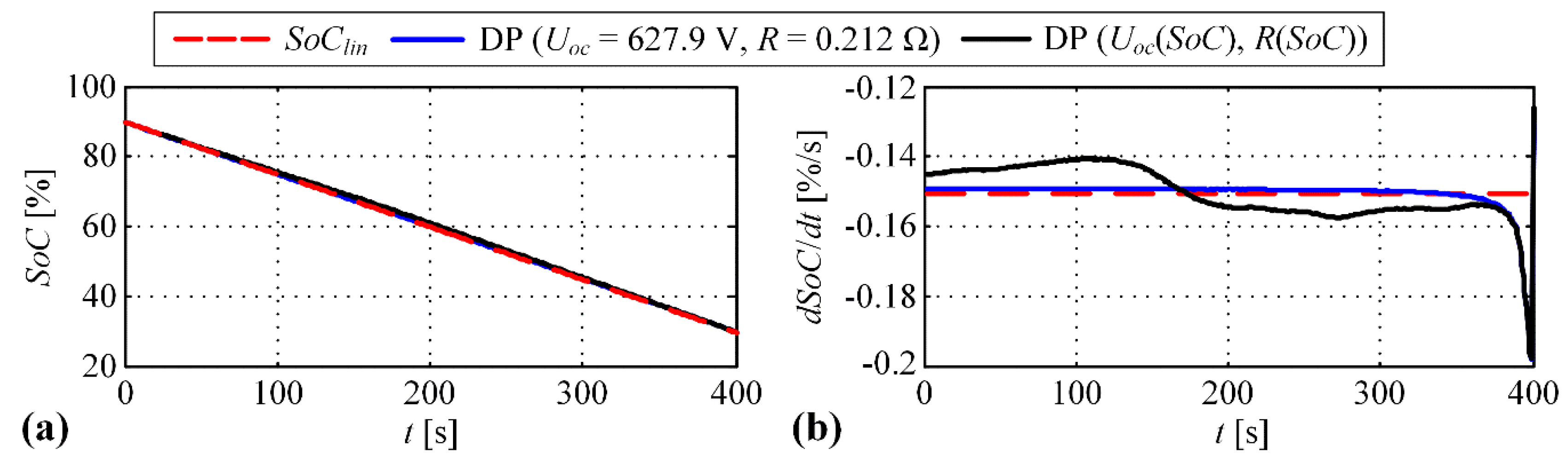
4.1. Simplified Case of Minimizing Solely Battery Energy Losses

First, the problem of discharging battery from the initial SoC value $So{C}_i$ (here $So{C}_i=0.9$) to some predefined final value $So{C}_f$ (here $So{C}_f=0.3$) with the aim of maximizing energy drawn from the battery is analyzed. The useful energy drawn is maximized if the internal battery energy losses $E_{batt,loss}$ are minimized:

$$\min E_{batt,loss}=\min \underset{0}{\overset{t_f}{{\displaystyle \int }}}{P}_{batt,loss}dt=\min \underset{0}{\overset{s_f}{{\displaystyle \int }}}\frac{P_{batt,loss}}{v_v}ds,\hspace{1em}\mathrm{s}.\mathrm{t}. \underset{0}{\overset{t_f}{{\displaystyle \int }}}\dot{SoC}dt=So{C}_f-So{C}_i.$$

(20)

The derivative of SoC with respect to travelled distance $s$ can be expressed as:

$$\frac{dSoC}{ds}=-\frac{I_{batt}\left(t\right)}{Q_{max}}\frac{1}{v_v}.$$

(21)

The battery power losses have quadratic dependence with respect to the battery current $I_{batt}$ described by the term $P_{batt,loss}=I_{batt}{}^{2}R\left(SoC\right)$, which is then combined with Equations (20) and (21), and finally resulting in the following optimization problem with $dSoC/ds$ serving as argument:

$$\underset{I_{batt}}{\min }\underset{0}{\overset{s_f}{{\displaystyle \int }}}\frac{I_{batt}^{2}R\left(SoC\right)}{v_v}ds=\underset{\frac{dSoC}{ds}}{\min }\underset{0}{\overset{s_f}{{\displaystyle \int }}}{Q}_{max}^{2}R\left(SoC\right){\left(\frac{dSoC}{ds}\right)}^2{v}_{v}ds, \mathrm{s}.\mathrm{t}. \underset{0}{\overset{t_f}{{\displaystyle \int }}}\dot{SoC}dt=So{C}_f-So{C}_i.$$

(22)

Discretization of Equation (22) leads to:

$$\underset{\frac{\mathsf{\Delta }So{C}_r}{\mathsf{\Delta }{s}_r}}{\min }{\displaystyle \sum }_{r=1}^{N_R}R\left(So{C}_r\right){\left(\frac{\mathsf{\Delta }So{C}_r}{\mathsf{\Delta }{s}_r}\right)}^2{v}_{v,r}\mathsf{\Delta }{s}_r,\hspace{1em}\mathrm{s}.\mathrm{t}. {\displaystyle \sum }_{r=1}^{N_R}\mathsf{\Delta }So{C}_r=So{C}_f-So{C}_i,$$

(23)

where $\mathsf{\Delta }So{C}_r$ is the SoC depletion on the $r$^th route segment of length $\mathsf{\Delta }{s}_r$, while $N_R$ is the total number of discrete route segments. The factor $Q_{max}^2$ is omitted in Equation (23) since it is constant and does not have influence on the optimization problem solution. Under the assumption of the battery internal resistance $R$, vehicle velocity $v_{v,r}$, and length of all route segments $\mathsf{\Delta }{s}_r$ will be constant, the optimization problem can be further simplified:

$$\underset{\frac{\mathsf{\Delta }So{C}_r}{\mathsf{\Delta }{s}_r}}{\min }{\displaystyle \sum }_{r=1}^{N_R}{\left(\frac{\mathsf{\Delta }So{C}_r}{\mathsf{\Delta }{s}_r}\right)}^2,\hspace{1em}\mathrm{s}.\mathrm{t}. {\displaystyle \sum }_{r=1}^{N_R}\mathsf{\Delta }So{C}_r=So{C}_f-So{C}_i.$$

(24)

This assumption related to the resistance $R$ is reasonable because it is relatively constant for a wide range of SoC values (see Figure 3b), while other assumptions are introduced here for the purpose of simplification and analysis. Since the quadratic function is convex, the following expression based on Jensen’s inequality can be established:

$$\frac{{{\displaystyle \sum }}_{r=1}^{N_R}{\left(\frac{\mathsf{\Delta }So{C}_r}{\mathsf{\Delta }{s}_r}\right)}^2}{N_R}\ge {\left(\frac{{{\displaystyle \sum }}_{r=1}^{N_R}\frac{\mathsf{\Delta }So{C}_r}{\mathsf{\Delta }{s}_r}}{N_R}\right)}^2,$$

(25)

where the numerator on the left-hand side of Equation (25) corresponds to the cost function of the optimization problem (24). Now, the minimum of the left-hand side of Equation (25), corresponding to equality of the left-hand side and right-hand side terms, is achieved for the constant value of $\mathsf{\Delta }So{C}_r/\mathsf{\Delta }{s}_r$ for all route segments. By combining the equality constraint from Equation (24) related to the SoC boundary values and posing $\mathsf{\Delta }So{C}_r/\mathsf{\Delta }{s}_r$ to be constant, the following expression for the optimal SoC depletion on r^th route segment is obtained:

$$\frac{\mathsf{\Delta }So{C}_r}{\mathsf{\Delta }{s}_r}=\frac{So{C}_f-So{C}_i}{s_f},$$

(26)

where $s_f$ represents the total travelled distance. In this case, the optimal battery operation would be to discharge the battery with constant SoC depletion rate, thus resulting in the SoC trajectory with linear shape of minimum length.

The same battery discharging problem is further analyzed by means of DP-based optimization in order to analyze the impact of varying battery parameters on SoC trajectory shape. Figure 8 shows SoC trajectories obtained by the constant SoC depletion rate ($So{C}_{lin}$) and by DP optimizations for: (i) the constant battery parameters (the mean values from Figure 3b are used), and (ii) the SoC-dependent battery parameters (Figure 3b). The optimization horizon is set to 400 s in order to enable battery discharging with feasible battery power (mean value of the battery power in this case is equal to 96.6 kW, while the upper limit is 150 kW). It should be emphasized that this is performed only for the purpose of analysis and it is not related to realistic road conditions.

In the case of constant battery parameters, the optimal operation is related to a constant SoC depletion rate (Figure 8b; slight deviation from the constant value in the case of DP occurs due to discretization effects and the requirement on the final SoC value). The results shown in Figure 8a point out that the impact of variable battery parameters on the optimal SoC trajectory shape is almost negligible. Figure 8b shows the optimal SoC depletion rate time profiles, where in the case of variable battery parameters SoC depletion rate slightly deviates from the constant value which is caused by the battery resistance dependence on SoC (cf. the battery resistance profile from Figure 3b with optimal SoC depletion rate).

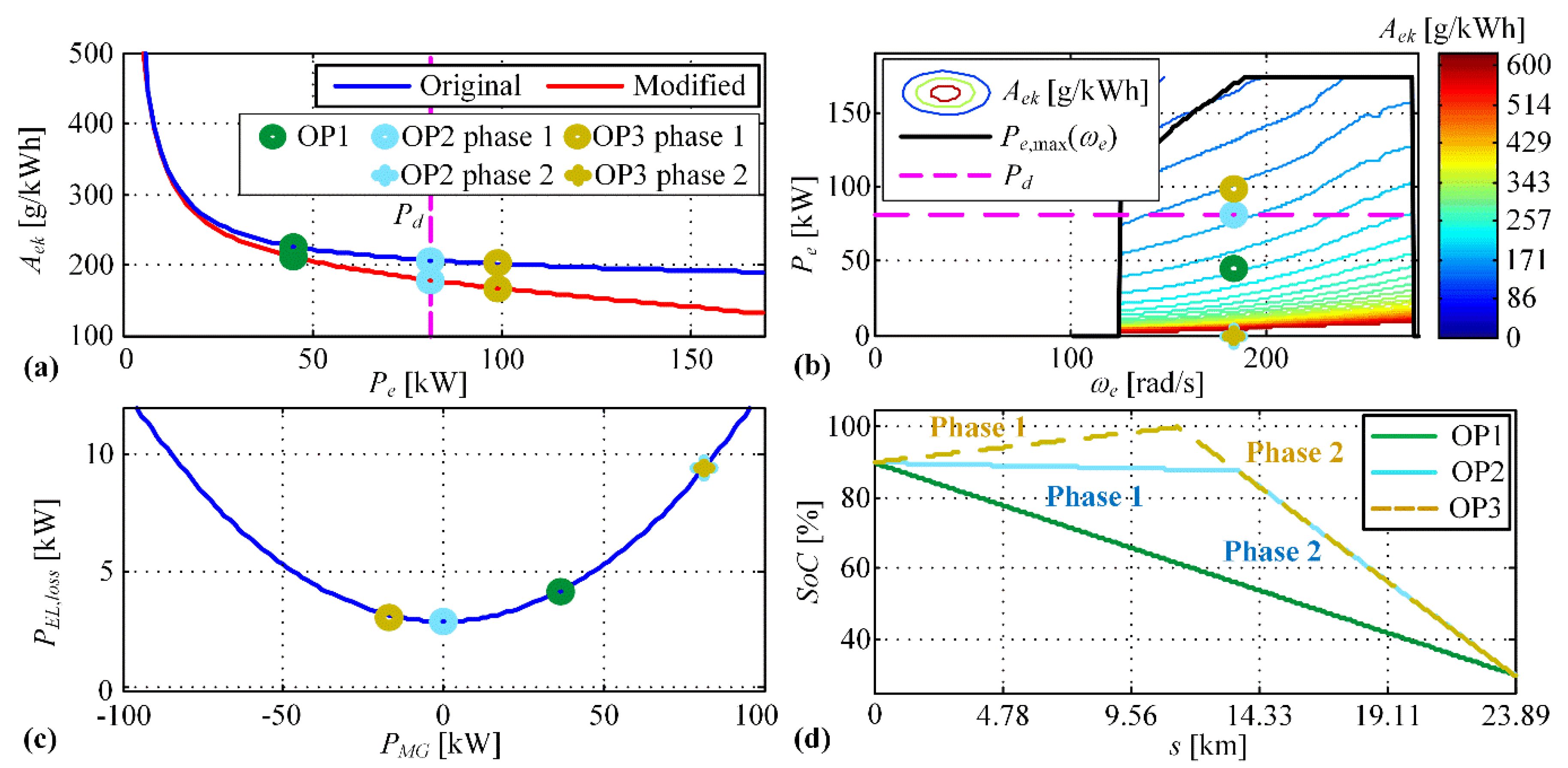
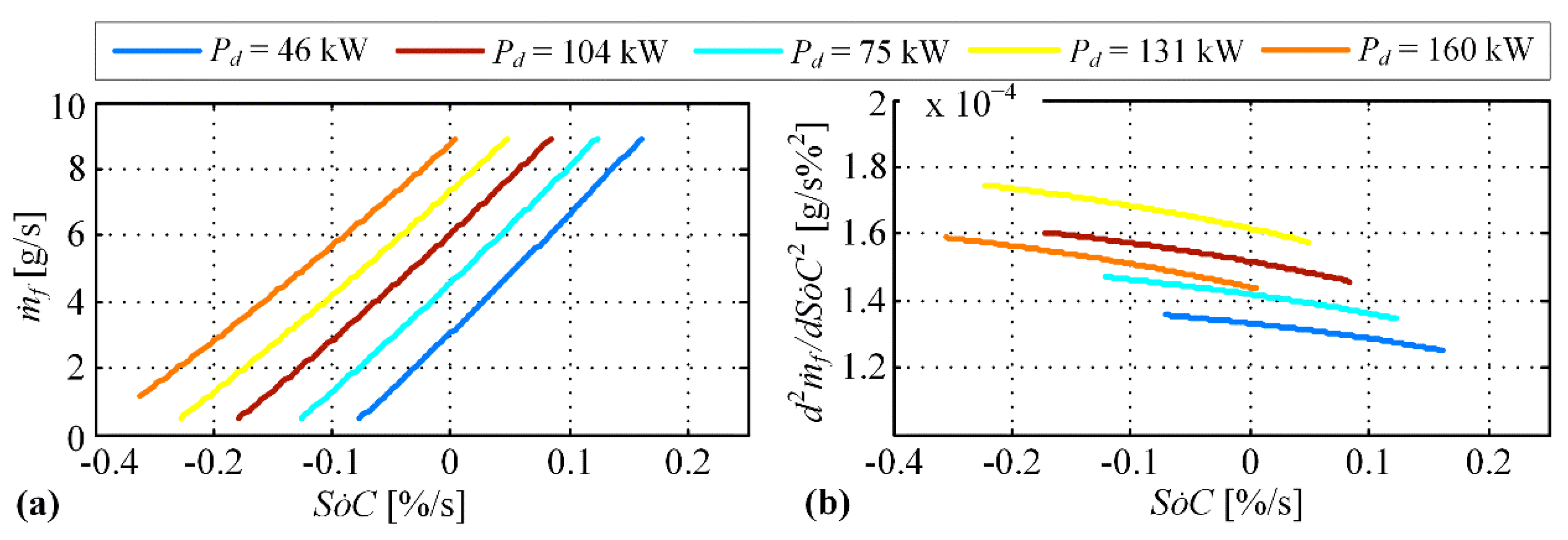
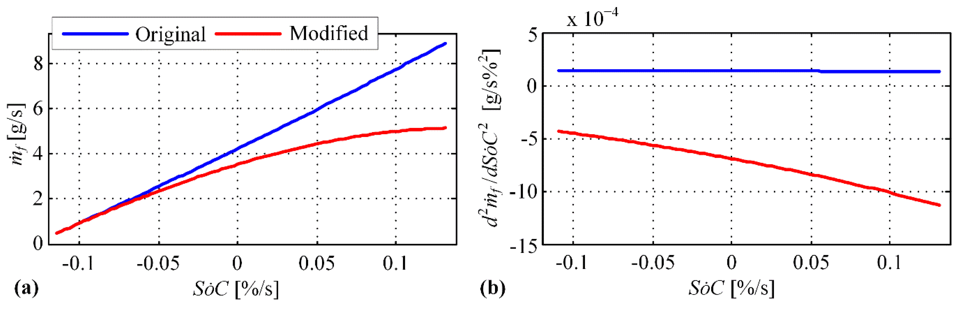
4.2. More Realistic Case of Minimizing Fuel Consumption

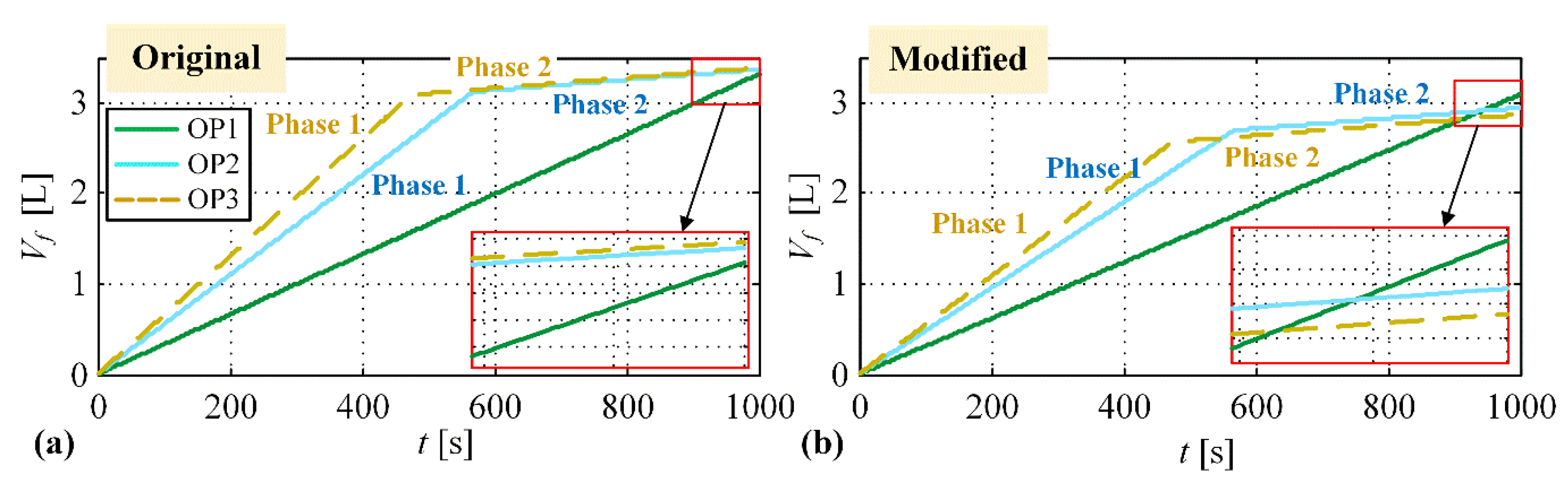
The analysis is extended here to the overall powertrain, which includes the engine, M/G machine, transmission, and battery (see Figure 1a). In order to study the optimal SoC trajectory with respect to fuel consumption minimization while discharging the battery (i.e., from 90% to 30%), the fuel consumption rate ${\dot{m}}_f$ is expressed in dependence on SoC depletion rate $\dot{SoC}$ for different values of the battery SoC, power demand $P_d$, and the engine speed ${\omega }_e$:

$${\dot{m}}_f=g\left(\dot{SoC},SoC,P_d,{\omega }_e\right).$$

(27)

The optimal solution for $\dot{SoC}$ which minimizes the total cumulative fuel consumption can be found analytically if the function $g$ in Equation (27) is convex, under assumption of constant values of $P_d$, $SoC$, and ${\omega }_e$(i.e., constant vehicle velocity). It can be shown that the optimality is achieved if $\dot{SoC}$ is kept constant during whole driving cycle and set to the value which would discharge the battery to the predefined minimum value (the same reasoning as in the case of deriving optimal SoC depletion in Equation (26)). The analysis is given here in the time domain, and it is equivalent to the travelled distance domain considered in previous sections because of the constant vehicle velocity assumption introduced here.

Figure 9a shows the graphical representation of the function (27) for several $P_d$ values and for $SoC$= 50%. The corresponding second derivatives are positive over the whole range thus confirming the convexity of the analyzed functions (Figure 9b). This convexity analysis is also conducted for a wide set of $P_d$ and ${\omega }_e$ values, and the results are shown in Figure 10 (the function is categorized as non-convex if its second derivative is not strictly positive). According to the results from Figure 10, the function $g$ in Equation (27) is convex for a majority of $P_d$ and ${\omega }_e$ values.

These effects are further illustrated and analyzed for the particular ${\omega }_e$ and $P_d$ values for two engine fuel consumption characteristics (g/s): (i) the original one (obtained from Figure 2a by using Equation (5)) resulting in the function (27) to be convex, and (ii) the modified one resulting in the function (27) to be concave (see Figure 11). Here, the modified engine specific fuel consumption map is introduced solely to demonstrate that the optimal SoC trajectory may differ from the linear one of minimum length depending on the convexity character of function (27).

Three different scenarios of battery discharging to the predefined low value of 30% are considered (see related operating points and profiles in Figure 12):

• OP1: power demand $P_d$ is partly satisfied by the engine and partly by the M/G machine (operating points are kept constant during the whole operation; constant $\dot{SoC}$ < 0),
• OP2—Phase 1: power demand $P_d$ is completely satisfied by the engine ($\dot{SoC}$ = 0), Phase 2: power demand $P_d$ is completely satisfied by the M/G machine (constant $\dot{SoC}$ < 0),
• OP3—Phase 1: power demand $P_d$ is completely satisfied by the engine which also provides additional power to recharge the battery (constant $\dot{SoC}>0$), Phase 2: power demand $P_d$ is completely satisfied by the M/G machine (constant $\dot{SoC}<0$).

From the standpoint of lower engine specific fuel consumption and regardless of type of engine fuel consumption characteristic (original or modified), Scenario OP2 is preferable over Scenario OP1, and Scenario OP3 is preferable over Scenario OP2 (see Figure 12a,b). However, from the standpoint of overall powertrain fuel consumption, Scenario OP1 related to linear SoC trajectory should be optimal if the function ${\dot{m}}_f$ vs. $\dot{SoC}$ is convex (as it is the case with the original characteristic shown in Figure 11a), while it should be suboptimal in the case of non-convex function (the modified characteristic shown in Figure 11a). This is confirmed by the results presented in Figure 13, where the comparative fuel consumption time profiles are shown for different scenarios. This finding can be explained by the fact that it is advantageous to place the engine operating point to somewhat larger specific engine fuel consumption (OP1 vs. OP2 and OP3, see Figure 12a) in the case of original engine characteristic, and thus avoid relatively large total electric losses whose increase is progressive with the M/G power (i.e., battery power, Figure 12c). In this case it is optimal to keep $\dot{SoC}$ constant which results in the SoC trajectory of minimum length. However, in the case of modified engine characteristic, where the difference in the specific fuel consumption between OP2 vs. OP1 and OP3 vs. OP2 is more significant than in the original case, it is advantageous to move the engine operating point in reduced specific fuel consumption region (OP3 and OP2; see Figure 12a,b) despite the increased electric losses in Phase 2 (Figure 12c).

The above analysis contributes to understanding of the tendency of optimal SoC trajectories to be of minimum length (as observed in Figure 5), taking into account that the function $g$ in Equation (27) is convex in a great majority of operating region (Figure 10) for the original engine specific fuel consumption map.

5. Conclusions

This paper has presented the analysis of the optimal battery state-of-charge (SoC) trajectory for the blended operating regime of a parallel plug-in hybrid electric vehicle (PHEV). The analysis was based on the optimization results obtained by using dynamic programming (DP) algorithm, for various driving cycles. It has been found that the optimal SoC trajectories expressed with respect to travelled distance tend to have nearly-linear (i.e. minimum-length) shape for different driving cycles. The linear SoC trajectory was also proven to be optimal both analytically and numerically for a simplified battery-only system based on battery power loss minimization. The analysis was extended to the whole powertrain including the engine, electric machine and battery, where the main aim was to minimize the total fuel consumption. It has been shown that the linear SoC trajectory is also optimal for the whole powertrain in the (actual) case of convex shape of engine fuel mass flow versus SoC depletion rate characteristic. It has been also demonstrated that when modifying the engine specific fuel consumption characteristic to some extent, the optimal SoC trajectory can have significantly different patterns than the minimum-length linear one.

In summary, the analyses conducted in this paper have pointed out that the minimum length linear SoC trajectory is optimal because of its feature to minimize the total electric losses and because of flexibility in setting the engine operating points due to a relatively flat engine specific fuel consumption vs. engine power characteristic in a wide range.

References

1. Miller, M.A.; Holmes, A.G.; Conlon, B.M.; Savagian, P.J. The GM “Voltec” 4ET50 Multi-Mode Electric Transaxle. SAE Int. J. Engines 2011, 4, 1102–1114. [Google Scholar] [CrossRef]
2. Škugor, B.; Cipek, M.; Deur, J. Control Variables Optimization and Feedback Control Strategy Design for the Blended Operating Mode of an Extended Range Electric Vehicle. SAE Int. J. Altern. Powertrains 2014, 3, 152–162. [Google Scholar] [CrossRef]
3. Yu, H.; Kuang, M.; McGee, R. Trip-Oriented Energy Management Control Strategy for Plug-In Hybrid Electric Vehicles. IEEE Trans. Control Syst. Technol. 2014, 22, 1323–1336. [Google Scholar]
4. Onori, S.; Tribioli, L. Adaptive Pontryagin’s Minimum Principle supervisory controller design for the plug-in hybrid GM Chevrolet Volt. Appl. Energy 2015, 147, 224–234. [Google Scholar] [CrossRef]
5. Soldo, J.; Škugor, B.; Deur, J. Optimal Energy Management Control of a Parallel Plug-in Hybrid Electric Vehicle in the Presence of Low Emission Zones. In Proceedings of the WCX SAE World Congress Experience, Detroit, MI, USA, 9–11 April 2019. [Google Scholar]
6. Martinez, C.M.; Hu, X.; Cao, D.; Velenis, E.; Gao, B.; Wellers, M. Energy Management in Plug-in Hybrid Electric Vehicles: Recent Progress and a Connected Vehicles Perspective. IEEE Trans. Veh. Technol. 2017, 66, 4534–4549. [Google Scholar] [CrossRef]
7. Ambuhl, D.; Guzzella, L. Predictive reference signal generator for hybrid electric vehicles. IEEE Trans. Veh. Technol. 2009, 58, 4730–4740. [Google Scholar] [CrossRef]
8. Liu, Y.; Li, J.; Qin, D.; Lei, Z. Energy management of plug-in hybrid electric vehicles using road grade preview. In Proceedings of the IET International Conference on Intelligent and Connected Vehicles (ICV 2016), Chongqing, China, 22–23 September 2016. [Google Scholar]
9. Bouwman, K.R.; Pham, T.H.; Wilkins, S.; Hofman, T. Predictive Energy Management Strategy Including Traffic Flow Data for Hybrid Electric Vehicles. IFAC-PapersOnLine 2017, 50, 10046–10051. [Google Scholar] [CrossRef]
10. Gaikwad, T.D.; Asher, Z.D.; Liu, K.; Huang, M.; Kolmanovsky, I. Vehicle Velocity Prediction and Energy Management Strategy Part 2: Integration of Machine Learning Vehicle Velocity Prediction with Optimal Energy Management to Improve Fuel Economy. In Proceedings of the WCX SAE World Congress Experience, Detroit, MI, USA, 9–11 April 2019. [Google Scholar]
11. Xie, S.; Hu, X.; Qi, S.; Tang, X.; Lang, K.; Xin, Z.; Brighton, J. Model predictive energy management for plug-in hybrid electric vehicles considering optimal battery depth of discharge. Energy 2019, 173, 667–678. [Google Scholar] [CrossRef]
12. Xie, S.; Hu, X.; Xin, Z.; Brighton, J. Pontryagin’s Minimum Principle based model predictive control of energy management for a plug-in hybrid electric bus. Appl. Energy 2019, 236, 893–905. [Google Scholar] [CrossRef]
13. Liu, K.; Asher, Z.; Gong, X.; Huang, M.; Kolmanovsky, I. Vehicle Velocity Prediction and Energy Management Strategy Part 1: Deterministic and Stochastic Vehicle Velocity Prediction Using Machine Learning. In Proceedings of the WCX SAE World Congress Experience, Detroit, MI, USA, 9–11 April 2019. [Google Scholar]
14. Soldo, J.; Škugor, B.; Deur, J. Optimal Energy Management and Shift Scheduling Control of a Parallel Plug-in Hybrid Electric Vehicle. In Proceedings of the Powertrain Modelling and Control Conference (PMC 2018), Loughborough, UK, 10–11 September 2018. [Google Scholar]
15. Guzzella, L.; Sciaretta, A. Vehicle Propulsion Systems, 2nd ed.; Springer: Berlin, Germany, 2007. [Google Scholar]
16. Bin, Y.; Li, Y.; Feng, N. Nonlinear dynamic battery model with boundary and scanning hysteresis. In Proceedings of the ASME 2009 Dynamic Systems and Control Conference, Hollywood, CA, USA, 12–14 October 2009; pp. 245–251. [Google Scholar]
17. Škugor, B.; Cipek, M.; Pavković, D.; Deur, J. Design of a power-split hybrid electric vehicle control system utilizing a rule-based controller and an equivalent consumption minimization strategy. Proceedings of the Institution of Mechanical Engineers, Part D. J. Automob. Eng. 2014, 228, 631–648. [Google Scholar]
18. Cipek, M.; Škugor, B.; Čorić, M.; Kasać, J.; Deur, J. Control variable optimisation for an extended range electric vehicle. Int. J. Powertrains 2016, 5, 30–54. [Google Scholar] [CrossRef]
19. Bellman, R.E.; Dreyfus, S.E. Applied Dynamic Programming; Princeton University Press: Princeton, NJ, USA, 1962. [Google Scholar]
20. Wang, X.; He, H.; Sun, F.; Zhang, J. Application Study on the Dynamic Programming Algorithm for Energy Management of Plug-in Hybrid Electric Vehicles. Energies 2015, 8, 1–20. [Google Scholar] [CrossRef]
21. Soldo, J.; Škugor, B.; Deur, J. Synthesis of Optimal Battery State of Charge Trajectory in the Presence of Varying Road Grade for a Parallel Plug-in Hybrid Electric Vehicle. In Proceedings of the 14th Conference on Sustainable Development of Energy, Water and Environment Systems (SDEWES), Dubrovnik, Croatia, 1–6 October 2019. [Google Scholar]
Figure 1. Parallel configuration of plug-in hybrid electric vehicles (PHEV) powertrain (a), transmission idle-mode power loss map (b), and mechanical efficiency map (c).
Wevj 10 00075 g001
Figure 2. Engine specific fuel consumption map (a), and electric machine (M/G) machine efficiency map (b), given along with maximum torque lines (denoted in blue).
Wevj 10 00075 g002
Figure 3. Battery equivalent circuit (a), and dependencies of open-circuit voltage and internal battery resistance with respect to battery state-of-charge (SoC) for a considered lithium iron phosphate battery (b).
Wevj 10 00075 g003
Figure 4. City bus driving cycle including vehicle velocity ( v v ) (a), road grade ( δ r ) (b), and passenger mass ( m p a s s ) (c) time profiles recorded in the city of Dubrovnik (DUB); and velocity time profile for heavy-duty UDDS driving cycle (HDUDDS) which assumes a zero road (d).
Wevj 10 00075 g004
Figure 5. Optimal SoC trajectories obtained by the dynamic programing (DP) algorithm in blended regime for repetitive DUB driving cycle with varying road grade (a) and zero road grade (b); and for repetitive HDUDDS driving cycle (c) (see Figure 4; in the case of DUB driving cycle varying passengers mass from Figure 4c is used).
Wevj 10 00075 g005
Figure 6. Visualization of cumulative cost function J i   (see Equation (16)) along with the optimal SoC trajectory S o C D P for the case of two additional SoC constraints (i.e., S o C c o n s t r   = 45% at 1/3 of total trip distance, and S o C c o n s t r   = 55% at 2/3 of total trip distance) and 4 x DUB driving cycle with a zero road grade.
Wevj 10 00075 g006
Figure 7. Set of DP optimal SoC trajectories of different lengths obtained by imposing an additional SoC constraint (14) (a); and corresponding total fuel consumption V f shown with respect to normalized SoC trajectory length L S o C , n o r m (b), mean engine specific fuel consumption A e k , m e a n (c), and total electric energy losses E E L , l o s s (d) (3 x DUB driving cycle when a zero road grade was used).
Wevj 10 00075 g007
Figure 8. SoC trajectories obtained by constant SoC depletion rate ( S o C l i n ) and by DP optimization for the constant and variable SoC-dependent battery parameters (a), and corresponding SoC depletion rates (b).
Wevj 10 00075 g008
Figure 9. Fuel consumption rate m ˙ f versus SoC depletion rate S o C ˙ (a), and second derivative of m ˙ f   versus S o C ˙   curve (b), given for several values of demanded power P d , engine speed ω e   = 184 rad/s and S o C   = 50%.
Wevj 10 00075 g009
Figure 10. Character of m ˙ f vs. S o C ˙   dependence (convex or non-convex) for a wide range of engine speeds ω e   and driver power demands P d   for the case of S o C   = 0.5.
Wevj 10 00075 g010
Figure 11. Illustration of original (convex) and modified (concave) engine fuel consumption rate m ˙ f   with respect to SoC depletion rate S o C ˙ (a), and the corresponding second derivatives (b) for the case of S o C   = 50%, v v   = 86 km/h, ω e   =   ω M G   = 184 rad/s, P d   = 79.7 kW.
Wevj 10 00075 g011
Figure 12. Illustration of three different operating scenarios through engine mean specific fuel consumption (a), engine power (b), total electric energy losses (c), and SoC trajectory profile (d) (the same operating conditions as in Figure 11: S o C = 50%, v v   = 86 km/h, ω e   =   ω M G   = 184 rad/s, P d   = 79.7 kW).
Wevj 10 00075 g012
Figure 13. Comparative cumulative fuel consumption time profiles for different operating scenarios for original (a) and modified engine fuel consumption characteristics (b).
Wevj 10 00075 g013