Optimal Incentives for Electric Vehicles at e-Park & Ride Hub with Renewable Energy Source

Abstract

As electric vehicles’ penetration increases, more impacts on urban systems are observed and related to both driving (e.g., on traffic congestion and reduced pollution) and charging (e.g., on the electrical grid). Therefore, there is a need to design coupled incentive mechanisms. To propose and numerically evaluate such incentives, a game theory model is adopted. Its originality comes from the coupling between the charging cost and the driving decisions: to drive downtown or to charge at an e-Park & Ride hub with solar panels and then take public transport, in order to reach destination. Optimal ticket fares and solar park’s size are computed using real photovoltaic production data.

1. Introduction

1.1. Motivation

At a local scale, urban well-being is sensitive to road usage and its impact on traffic congestion, local air pollution and noise. Electric vehicles (EV), considering both battery and plug-in hybrid technologies, are a promising solution to these issues. However, the forecasted high penetration of EV (see middle scenario in [1]) may lead to local grid constraints, e.g., transformers aging and power losses. Even if the penetration rate of EV is not yet really significant at the national scale, it can already be substantial at a local scale (see e.g., the case of “Île-de-France”, with more than 20,000 EV in circulation: http://www.automobile-propre.com/dossiers/voitures-electriques/chiffres-vente-immatriculations-france/, in French). This “grid congestion” problem has to be considered as a key factor for the large scale deployment of EV. Therefore, a model to evaluate coupled driving-and-charging incentives for EV can be very useful to understand and predict future performances of such complex interaction between transport and energy. The flexibility of EV charging—in terms of compatibility with end users’ mobility needs and technical capabilities for load management—makes it a significant tool in “Demand Response” mechanisms [2] which is an emerging field in “Smart Grids”. Such scheduling techniques consist in shifting/adapting the consumption profile by, e.g., postponing usages in time, or reducing the level of power consumed, with different objectives for the electrical system: local management of production-consumption balance, mitigating the impact on the electrical grid [3], etc. This is totally innovative compared to the traditional paradigm of the electrical system, where almost only generation units were flexible to ensure its effective operation. (For other tasks than EV charging like heating, cooking and so on, there is less potential to “smartly” schedule the associated electricity consumption profile. Currently, the main flexibility in France is water-heating, controlled through on/off-peak fares.) In this context, taking into account charging strategies into everyday EV driving decisions will become an important issue in smart cities, particularly for urban networks [4]. Another important problem is the design of charging incentives (e.g., under the form of pricing or services) to share—in space and time—public EV Charging Stations (or EVCS) [5].

To solve these problems, EV driving decisions must also be taken into account. This coupling is clearly observable during widespread holiday journeys or particular events: the majority of driving EV need to charge at public EVCS, where there could be a significant waiting time and available power reduction (when allocated/shared between plugged EV) due to simultaneous power demands. As an example of incentive mechanism, Tesla EVCS proposes a differentiated service and adapts the charging prices in order to encourage EV to charge in empty EVCS rather than congested ones (https://www.tesla.com/support/supercharging). Another example from the French company Compagnie Nationale du Rhône (CNR) is the “Move In Pure” charging subscription: in order to guarantee an EV charging green power sourcing, drivers are incited to charge at specific hours of the day (resp. locations) when (resp. where) renewable energy is available. In a more futuristic vision, the EV charging-and-driving coupling can be transposed into a charging-by-driving one, with an inductive charging system (under the road) as suggested in [6]. Finally, Park & Ride hubs—associated with public transport—are in vogue to mitigate congestion and local pollution in urban areas: up to 18,000 parking spaces are expected at Paris gates by 2021 (www.iledefrance-mobilites.fr/actualites/18-000-places-de-parc-relais-2018/). This multimodal alternative solution represents a great opportunity for smart charging. The model presented in this work takes into account this coupled framework between EV driving and charging decisions in order to offer an accurate representation of EV behavior. A direct application of the proposed model allows testing incentives aimed at, e.g., mitigating the impact of EV charging on the electrical grid, minimizing the proportion of gasoline vehicles into city center or maximizing the profit of charge point operators (CPO). Having this context in mind, we propose a scenario in which a population of electric and gasoline vehicles follow the same journey from a sub-urban area to a city center, which corresponds to regular commuting patterns.

1.2. Related Methodologies

Basic traffic assignment problem (TAP) with single-class drivers (meaning that there is only one type of vehicle) is defined and studied in [7]. Under certain conditions (drivers equally affected by traffic congestion and increasing cost functions), it is shown that there is a unique solution (the solution concept, explained in next section, is close to the Nash equilibrium concept in game theory) to this problem. In recent years, there has been an increasing interest for mixed TAP where two or more classes of vehicles are considered [8] (e.g., electric and gasoline vehicles). The uniqueness of the solution in mixed TAP is proved in [9] when the cost functions are the same for every driver, up to an additive constant.

On the charging side of the problem, the water-filling schedule of [10] will be used. The coupling of the driving and charging problems is studied in particular in [11,12]. However, [11] focuses only on a single class of vehicles and [12] considers that the EV charging need is constant and does not depend on their driving decisions.

2. E-Park & Ride Hub Scenario

Note that the scenario considered here is one of the many practical applications of the generic model developed in our previous work [13]. This work focuses typically on daily commuters who want to get to their workplace in the morning: they come from the suburb area (Origin O in Figure 1) and head to the city center (Destination D). This city is concerned with traffic congestion and local pollution, so an e-Park & Ride hub is built on the outskirts of the city to limit the number of vehicles downtown. In this scenario, when commuters arrive at the hub, they can choose between two transport modes. First, they can park at the hub and finish their trip by public transport ($publ$ in Figure 1). Second, they can drive past the hub into the city center with their private vehicle ($priv$). At the hub, a charge point operator (CPO) is in charge of smart public EVCS and PhotoVoltaic (PV) solar panels. Usually, the CPO is separate from the network operators of the electrical grid and the traffic network. Here for simplicity it is assumed that the same operator (still called CPO) is in charge of the EVCS, the PV panels, and the electrical grid. The relationships between the three operators have not been considered because our work is focused on EV drivers’ decisions and their impact. However, these higher level economic relationships between the CPO and network operators can be added on top of our model, which will be the focus of future works.

Note that while the private transport mode may be faster, the public one may be cheaper thanks to incentives, like public transport ticket fare discount or cheaper charging service for EV due to a local electricity production at the hub. The aim of this work is to model and then to predict the choice of commuters and to find how it may be affected by various incentives like the two mentioned above.

2.1. Route Choice

2.1.1. Model Assumptions

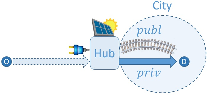
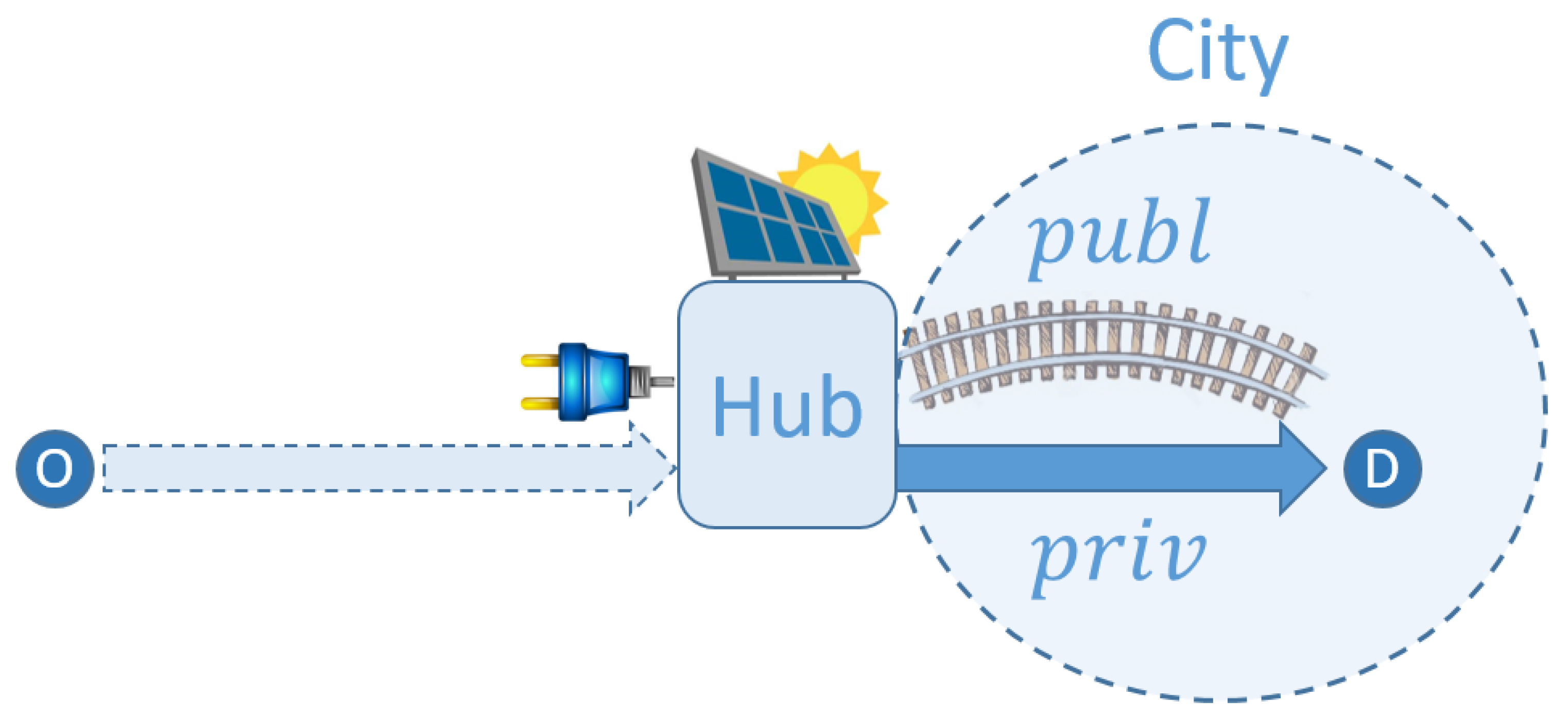
• Two types of vehicle are considered: an electric one (denoted EV and associated with subscript e) and a gasoline one (GV, associated with subscript g). Each commuter is associated with one of the two vehicles and the proportion of EV among them is denoted by $X_e$ in the model (in numerical tests, $X_e=50\%$ which is in line with 2035 predictions for France; see middle scenario of [1]). The proportion of GV is then given by $X_g=1-X_e$. The choice made by all commuters between the two transport modes of Figure 1 is represented by the two variables $x_{e,publ}$ and $x_{g,publ}$, which are respectively the proportions of EV and GV choosing the public transport mode. Note that the proportions of vehicles of type $s=e,g$ choosing the private transport mode may be easily deduced: $x_{s,priv}=1-x_{s,publ}$.
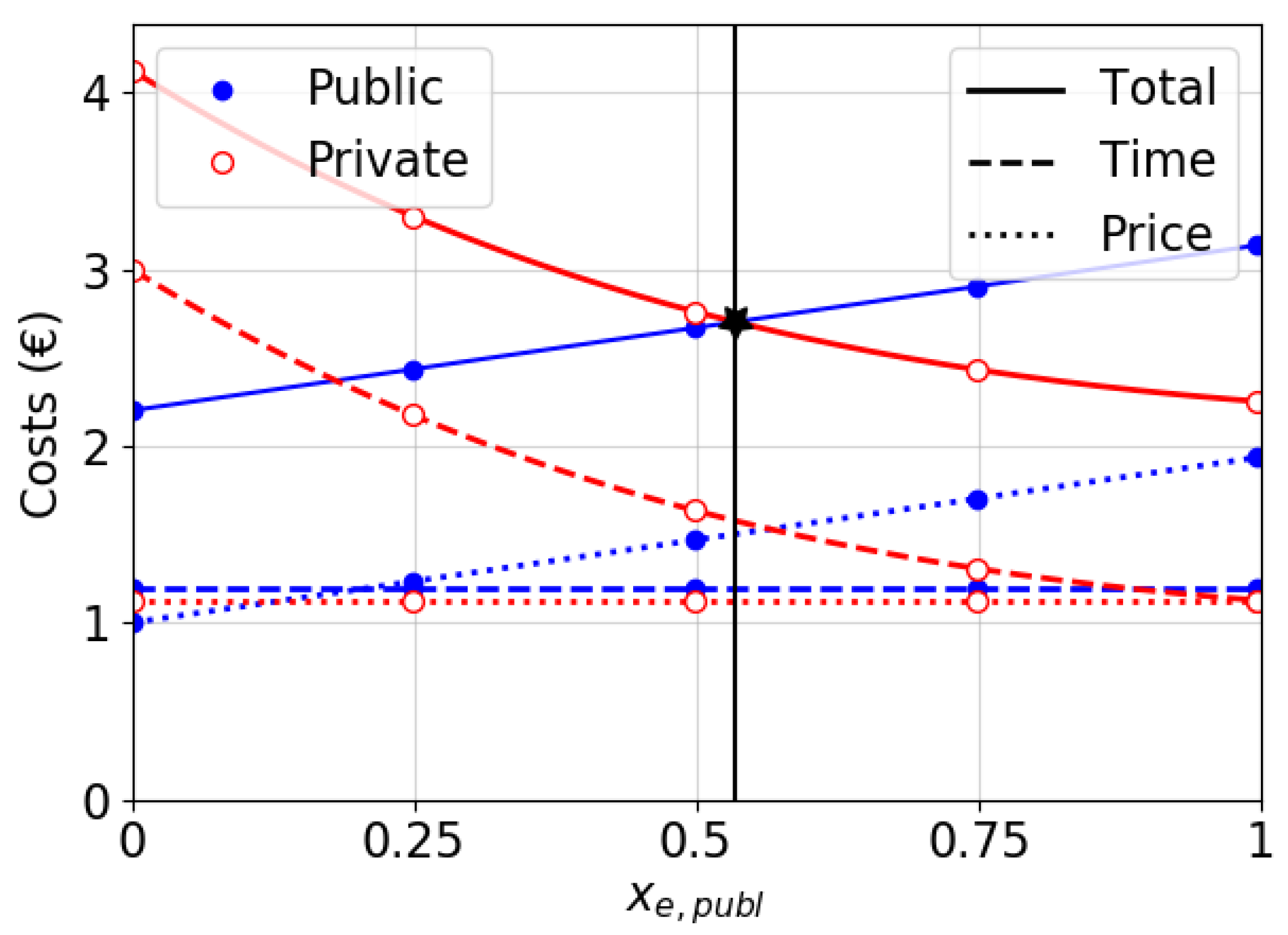
• The decision process of commuters is assumed rational, meaning that they choose the transport mode (publ or priv) with minimal cost. Here, the costs considered are travel duration (by private or public transport), energy consumption (electricity for EV and fuel for GV) and the ticket fare (for public transport only).

2.1.2. Costs Functions

The first type of cost considered is related to travel duration and/or delay from the hub to the destination, which is perceived equivalently by EV and GV:

(a) Travel Duration Costs

–

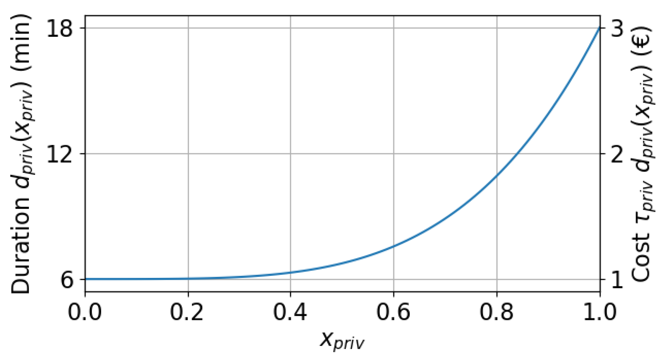
For the private mode, it depends on the total proportion (here, proportion and number of vehicles are equivalent, as the total number of vehicles is fixed) of vehicles driving downtown $x_{priv}=x_{e,priv}{X}_e+x_{g,priv}{X}_g=(1-x_{e,publ})X_e+(1-x_{g,publ})X_g$ due to congestion effects [14] and is expressed as:

$${\tau }_{priv}\times \underset{d_{priv}\left(x_{priv}\right)}{\underbrace{\frac{l}{v}\left(1+2{\left(\frac{x_{priv}}{C}\right)}^4\right)}},$$

(1)

where the function $d_{priv}(.)$ is the estimated travel duration on the road downtown: the higher the flow $x_{priv}$, the higher the travel duration and $x_{priv}=0$ yields the (minimal) “free-flow” travel time. The parameters of the problem are set as follows, unless otherwise specified:

• ${\tau }_{priv}=10$ €/h the value of time when driving, based on a French government report (http://www.strategie.gouv.fr/sites/strategie.gouv.fr/files/archives/Valeur-du-temps.pdf),
• $l=5$ km the length of the road, approximately the radius of Paris,
• $v=50$ km/h the speed limit, as in French urban areas,
• $C=1$ the capacity of the road, expressed in proportion of the total number of vehicles, like $x_{priv}$.

Note that if all vehicles choose to drive downtown ($x_{priv}=1$), the corresponding travel duration is multiplied by three compared to the empty road situation (or free-flow) due to traffic jams (see Figure 2) (a typical value for inter-urban areas [15]).

–

For the public transport mode linking the hub and the destination, the travel cost is assumed constant:

$${\tau }_{publ}\times d_{publ},$$

(2)

• ${\tau }_{publ}=12$ €/h value of time in public transport (http://www.strategie.gouv.fr/sites/strategie.gouv.fr/files/archives/Valeur-du-temps.pdf), which is perceived by commuters as less comfortable than personal vehicles,
• $d_{publ}=\frac{l}{v}=6$ min constant travel time of public transport, which was chosen equal to the free flow travel time of the private mode. Indeed, there exist reserved pathways for public transportation in several cities like Paris, so that congestion can be considered as marginal.

The duration cost of the public mode is then equal to the fixed value ${\tau }_{publ}{d}_{publ}=1.2$ € and is higher than the free flow cost of the private mode. This induces trade-off decisions for vehicles between both strategies.

(b) Energy Consumption Cost

It corresponds to the energy consumed by the vehicle from the origin to the destination; it is different for EV and GV. The expression of this cost for vehicles of type $s=e,g$ which have chosen transport mode $r=publ,priv$ is as follows:

$$l_r\times m_s\times {\lambda }_s.$$

(3)

Note that here, the consumption model is assumed to be distance-dependent.

• $l_r$ is the total distance driven by the vehicles which have chosen transport mode r, and is equal to:

  –

  $l_{publ}=10$ km distance between the origin and the hub, so that the two-way trip between origin and destination is 30 km, the daily average individual driving distance in France (following Enquête Nationale Transports et Déplacements: https://utp.fr/system/files/Publications/UTP_NoteInfo1103_Enseignements_ENTD2008.pdf), 2008, in French),

  –

  $l_{priv}=l_{publ}+l=15$ km,

• $m_s$ is the electricity or fuel consumed per distance unit and is supposed constant (e.g., it does not depend on speed profiles):

  –

  $m_e=0.2$ kWh/km, following [16],

  –

  $m_g=0.06$ L/km (Liter/km),

• ${\lambda }_s$ is the charging/fueling unit price:

  –

  For EV, the key distinction made here is that it depends on the transport mode chosen.

  Public mode: At the hub, this charging unit price ${\lambda }_e$ will depend on the total charging need $L_e\left(x_{e,publ}\right)$, proportional to the number of EV parked in the hub: for example, if there are few EV at the hub ($x_{e,publ}$ close to 0), there is enough electricity produced at the hub to provide the charging need of these EV. This price is obtained by solving a charging problem, which is detailed in the next section.

  Private mode: Downtown, there is a standard constant electricity fare ${\lambda }_e^0=$ 40 c€/kWh, which corresponds to the electricity unit price in France (15 c€/kWh) with an additional cost (25 c€/kWh) meant for the charging operation.

  –

  ${\lambda }_g=1.50$ €/L is considered constant.

(c) Public Transport Ticket Fare

It is the same for EV and GV: $t_{publ}=1$€.

Finally, the total costs for each type $s=e,g$ of vehicle which have chosen transport mode $r=publ,priv$ are given in

Table 1. The total costs for EV and GV in different transport mode.

Total Costs	Public Transport Mode	Private Transport Mode
EV	$\begin{array}{c}{c}_{e,publ}\left(x_{e,publ}\right)={\tau }_{publ}{d}_{publ}+t_{publ}\\ {}_{}+l_{publ}{m}_e{\lambda }_e\left(L_e\left(x_{e,publ}\right)\right)\end{array}$	$\begin{array}{c}{c}_{e,priv}\left(\mathbf{x}\right)={\tau }_{priv}{d}_{priv}\left(x_{priv}\right)\\ {}_{}+l_{priv}{m}_e{\lambda }_e^0\end{array}$
GV	$\begin{array}{c}{c}_{g,publ}={\tau }_{publ}{d}_{publ}+t_{publ}\\ +l_{publ}{m}_g{\lambda }_g\end{array}$	$\begin{array}{c}{c}_{g,priv}\left(\mathbf{x}\right)={\tau }_{priv}{d}_{priv}\left(x_{priv}\right)\\ {}_{}+l_{priv}{m}_g{\lambda }_g\end{array}$

(where $\mathbf{x}=\left(x_{e,publ},x_{g,publ}\right)$).

Note that the driving and charging operations are coupled: the mode choice depends on the charging cost (charging impacts driving) while the EV charging need depends on their driving consumption (driving impacts charging).

According to the rationality assumption, each commuter chooses the transport mode with minimal total cost, under complete information: he knows all the total cost expressions presented in the previous table and know that all the other commuters want to minimize their total cost too. By all acting rationally in this sense, commuters will reach a certain distribution of choices between the public and the private modes. Such a distribution is denoted by ${\mathbf{x}}^{*}=\left(x_{e,publ}^{*},x_{g,publ}^{*}\right)$ and is called a Wardrop Equilibrium (or WE in game theory literature) [17]. This equilibrium situation gives a model of commuters’ behavior in a stable regime where no commuter has an interest to change his choice unilaterally. This is a typical situation, after some learning periods, when drivers determine their route or follow a guidance app, for their everyday journey from their home to their job. The proposed approach can thus be used to evaluate various incentive mechanisms numerically—in a planning stage or tool—in order to “select” a particular equilibrium before it will be observed in practice (observe that this concept is now commonly used in many operational public transportation planning tools for the “route choice” step in four-steps models), as done in Section 3.

Before that, the next section introduces the hub charging operation and the determination of the charging unit price in more detail.

2.2. Hub Charging Operation

This section explains how the charging unit price ${\lambda }_e$ at the hub is determined optimally and depends on the proportion of EV choosing the public transport mode, and thus charging at the hub.

2.2.1. Charging Scenario

When commuters arrive at the hub, those having an EV leave it plugged in during work hours and let the CPO choose the charging schedule (“centralized optimization problem”). For example, the CPO might refer to a state entity which built a smart charging infrastructure in order to minimize social costs, or to a private company opening its parking lot to the public. The CPO determines the individual charging profiles of all EV connected at the hub during the day. Here, instead of solving this optimal scheduling problem with the per-EV profiles—which is a topic in itself, see e.g., ref. [18], an aggregate version of this problem is tackled. It consists in considering an optimization problem in which the variable is the aggregated charging profile, i.e., the sum of the individual ones. With a significantly lower complexity of resolution (an explicit solution is available), it provides a good approximation of the aggregate charging cost, from which the charging unit price is derived. On top of that, the hub owns a local source of energy like photovoltaic (or PV) panels. Therefore, performing most of the charging operation around noon when PV panels are at their production peak may be a better solution for the CPO rather than a uniform charging profile. At the end of the day, the total cost/impact of the charging operation affects the hub charging unit price such that the CPO is at a break even point.

2.2.2. Modeling of Charging Problem

Aggregated Charging Need

It is assumed that before leaving the suburb areas (corresponding to the Origin on Figure 1), all EV’s state of charge is full, so that their charging need corresponds exactly to the electricity consumed during their trip from their origin to the hub. This assumption may be lifted by grouping the vehicles with the same initial state of charge. As the consumption model is distance-dependent, the aggregated charging need $L_e\left(x_{e,publ}\right)$ for all EV is then proportional to the total traveled distance $l_{publ}{x}_{e,publ}$ by the EV choosing the public transport mode:

$$L_e\left(x_{e,publ}\right)=l_{publ}{m}_e{x}_{e,publ}.$$

(4)

The CPO commits to fully charge all EV at the hub, i.e., the whole aggregated charging need $L_e$.

Temporal Charging Scheduling

The CPO determines which portion of the total charging need $L_e$ has to be charged during each working hour of the day in order to minimize total charging costs. Note that these costs are supposed to be aligned with the costs/impact of the charging operation on the electrical grid (introduced later in this section); in practice, a specific electricity contract would be signed between the CPO and the grid operator, determining the remuneration of the CPO for such “effort” (in France see the “Offres de Raccordement Intelligentes” by Enedis for an example of such a remuneration scheme). To simplify, the charging operation is assumed to take place only between 9 a.m. and 5 p.m., when all the EV which have chosen the public transport mode are likely to be plugged in (considering a hub with enough capacity). EV arriving at the hub before 9 a.m. or leaving after 5 p.m. will not be charged outside this period, so that the scheduling in this work might not be exactly optimal and the resulting charging unit price might be overestimated. The charging period consists in eight time slots of one hour each and the CPO decides the load ${\ell }_{e,t}$ to charge during each time slot $t\in \{1,\dots ,8\}$, so that the aggregated charging need is satisfied:

$$\sum _{t=1}^8{\ell }_{e,t}=L_e\left(x_{e,publ}\right)(\mathrm{in}\mathrm{kWh}).$$

(5)

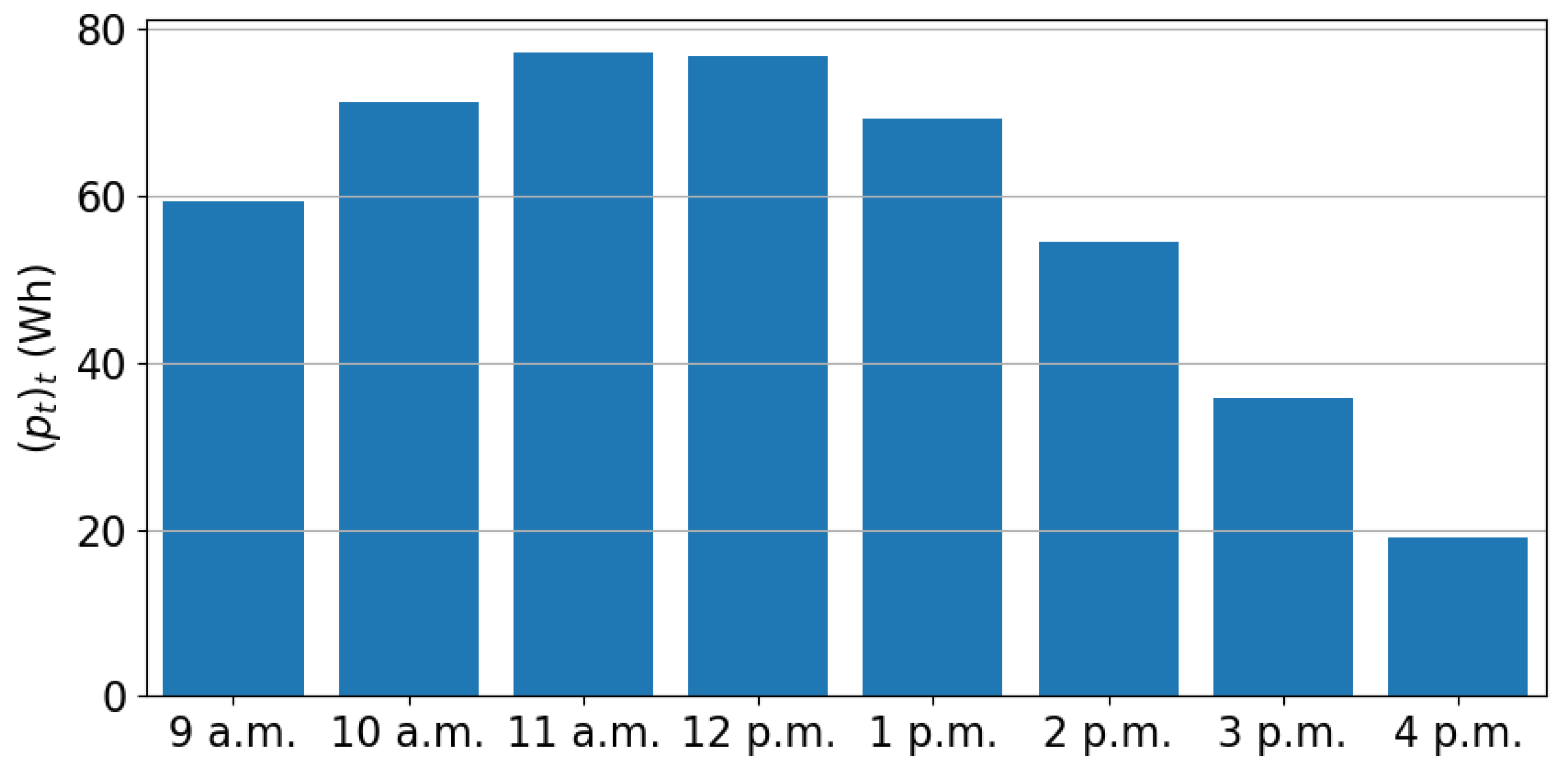
Photovoltaic Production

The CPO determines the aggregated charging profile taking into account its local PV energy production (assuming the PV production of the day is known when solving the charging problem, typically “just before” 9 a.m.). For each time slot $t\in \{1,\dots ,8\}$, the PV energy produced at the hub is denoted by $p_t\ge 0$. Figure 3 shows the open source data (available at https://www.renewables.ninja/) from [19] considered for the PV production. This figure shows the energy produced each working hour (averaged over the year 2014) per square meter of a regular photovoltaic panel (with a nominal power of 360 Wp and a surface of 2.06 m${}^2$) located in Paris (example taken from https://us.sunpower.com/solar-resources/products/datasheets/).

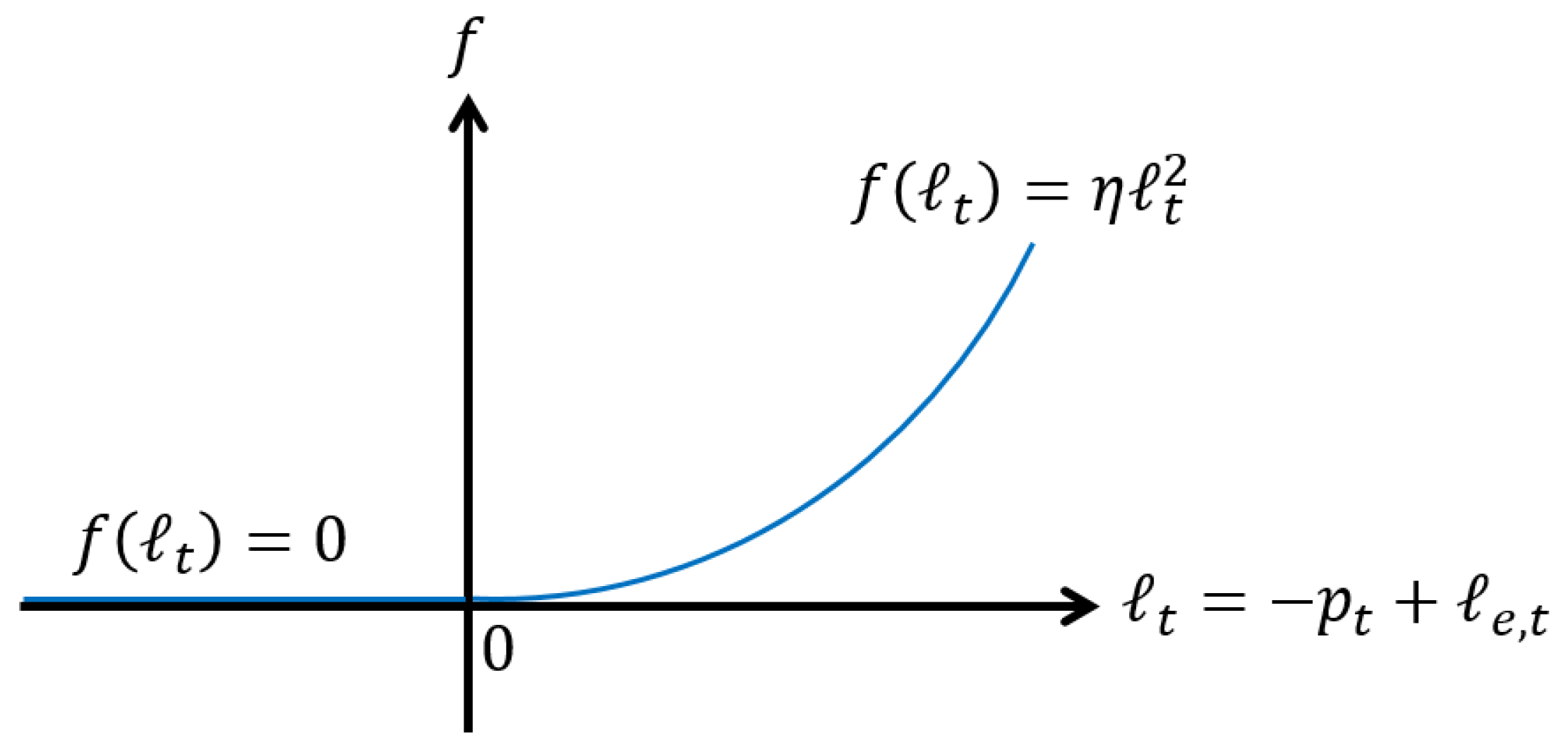
Cost/Impact on the Local Electrical Grid

The cost/impact of the charging operation on the local electrical (distribution) grid at time slot $t\in \{1,\dots ,8\}$ depends on the net load (“seen” from the grid) ${\ell }_t=-p_t+{\ell }_{e,t}$; it writes:

$$f\left({\ell }_t\right)=\left\{\begin{array}{cc}0\hfill & \mathrm{if}{\ell }_t\le 0,\hfill \\ \eta {\ell }_t^2\hfill & \mathrm{if}{\ell }_t>0.\hfill \end{array}\right.(\mathrm{in}€)$$

(6)

This cost is typically quadratic when the net load is positive and zero if not (see Figure 4). This form of function means that: when the charging operation uses only PV production, there are no grid costs: when the CPO needs electricity from the grid (i.e., ${\ell }_{e,t}>p_t$), costs are considered under an increasing and convex form standardly used in optimization/game-theory smart grid models to represent local grid congestion effects [10]. Following are a few observations regarding this grid cost modeling: 1. Regarding the particular choice of a quadratic function, note that the following study is still valid with more general monomials (cost function f with a higher degree); 2. Because the cost function in (6) does not depend on the variables at the other time slots (in particular on the previous net load ${\ell }_{t-1}$), this “proxy” does not include dynamical (e.g., transformer temperature inertia as in [3]) nor locational effects; 3. A local electricity storage for PV production is not considered here; its presence could decrease the net load and, in turn, the impact on the grid of (6); 4. Finally, this cost function incites the CPO to maximize the self-consumption of its PV production; this fact will be detailed further.

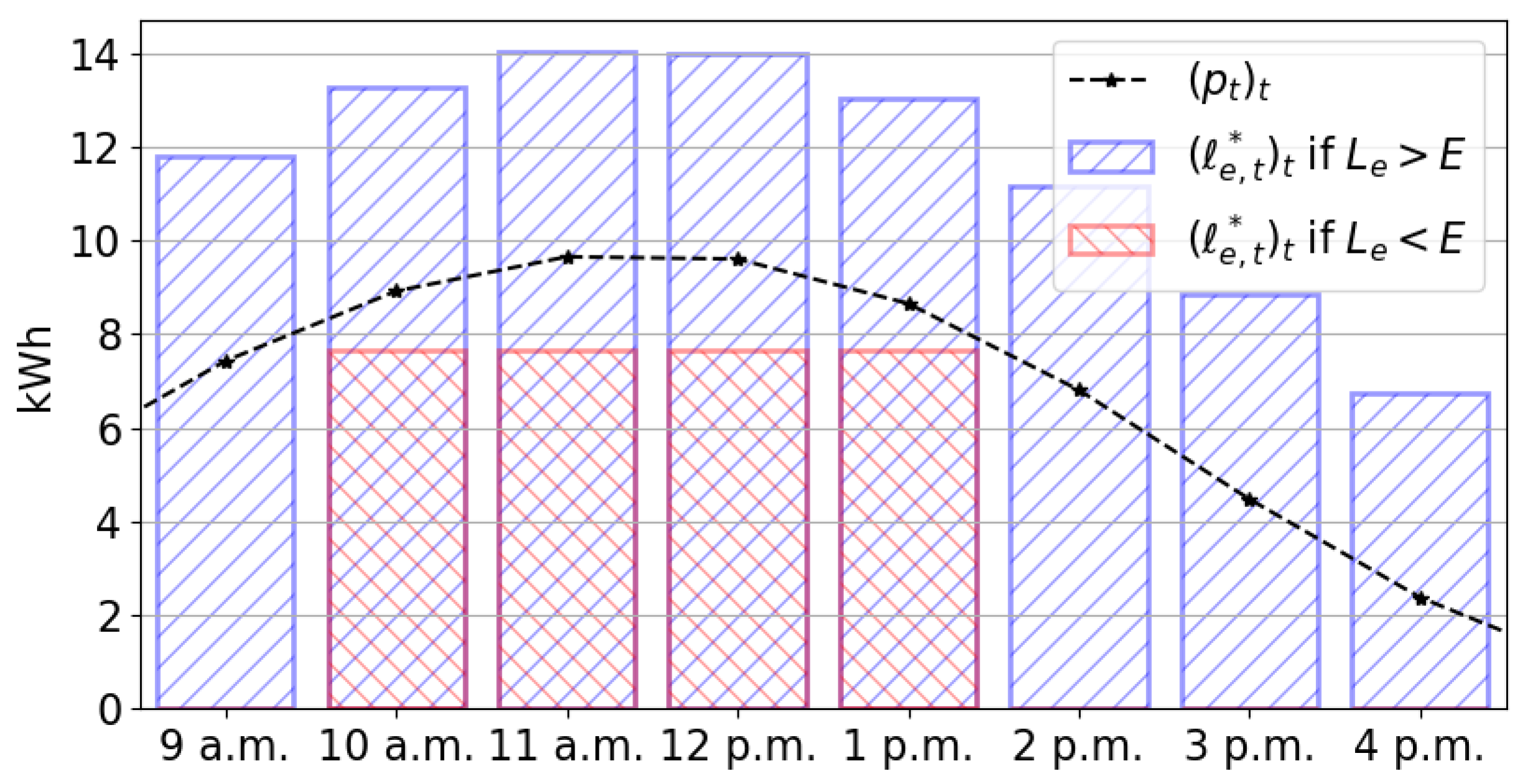
Charging Problem and Solution

Formally, the charging problem solved by the CPO writes:

$$\underset{{\left({\ell }_{e,t}\right)}_t}{min}\sum _{t=1}^{8}f\left(-p_t+{\ell }_{e,t}\right),\mathrm{s}.\mathrm{t}.\left\{\begin{array}{c}\forall t,{\ell }_{e,t}\ge 0,\hfill \\ \sum _{t=1}^8{\ell }_{e,t}=L_e\left(x_{e,publ}\right).\hfill \end{array}\right.$$

(7)

The solution of this problem only depends on the total PV energy produced during working hours $E={\sum }_{t=1}^8{p}_t$ (relatively to $L_e$) and not on the profile ${\left(p_t\right)}_t$ shape. To illustrate that, in Figure 5, the PV profile considered corresponds to a PV panel surface of 125 m${}^2$ (equivalent to the area of approximately 10 parking spots, or a nominal power of 21.9 kWp), with a mean (average over working days) total production of $E=57.9$ kWh during working hours per day.

• If the aggregated charging need $L_e\left(x_{e,publ}\right)$ verifies $L_e<E$, any charging profile below the PV production is optimal, since the associated cost is zero.
• If $L_e=E$ (which corresponds to the charging need of 29 EV), the optimal scheduling has to perfectly match the production.
• If $L_e>E$, all PV production is consumed and the remaining charging need has to be equally shared between all time slots such that the net load taken from the grid is constant.

The optimal charging schedule solution of (7) gives a minimal total cost/impact on the electrical grid denoted by $C\left(L_e\right)$ (in €), which is equal to (this minimal total cost C corresponds to the value function concept in optimization):

$$C\left(L_e\right)=\left\{\begin{array}{cc}0\hfill & \mathrm{if}{L}_e\le E,\hfill \\ \frac{\eta }{8}{\left(-E+L_e\right)}^2\hfill & \mathrm{if}{L}_e>E.\hfill \end{array}\right.$$

(8)

Having optimally scheduled the aggregated charging need $L_e\left(x_{e,publ}\right)$ in different time slots, the CPO then determines the charging unit price (for $L_e>0$) as follows:

$$\begin{array}{c}\hfill {\lambda }_e\left(L_e\right)={\lambda }_{\mathrm{cst}}+\frac{C\left(L_e\right)}{L_e}(\mathrm{in}€/\mathrm{kWh}),\end{array}$$

(9)

with ${\lambda }_{\mathrm{cst}}=20$ c€/kWh ($=\frac{{\lambda }_e^0}{2}$) a fixed charging fee. This way, the CPO makes EV pay equally (per energy unit) for the total charging cost caused by their aggregated electricity consumption need. Note the threshold role played by the total PV production E during working hours: ${\lambda }_e$ depends on the total charging need $L_e\left(x_{e,publ}\right)$ only if E is not sufficient to provide for $L_e$; otherwise the charging unit price is constant, equal to ${\lambda }_{\mathrm{cst}}$.

The parameter $\eta =4$ €/kWh${}^2$ was adjusted so that the maximal charging unit price ${\lambda }_e$ at the hub (with ${\lambda }_{\mathrm{cst}}=0$), which occurs when there is no PV production ($E=0$) and all EV choose public transport and thus charge at the hub ($L_e^{\max }=l_0{m}_e{X}_e$), is equal to $\frac{5}{4}{\lambda }_e^0=50$ c€/kWh. Note that this maximal price is higher than the fixed price downtown ${\lambda }_e^0$.

3. Numerical Experiments

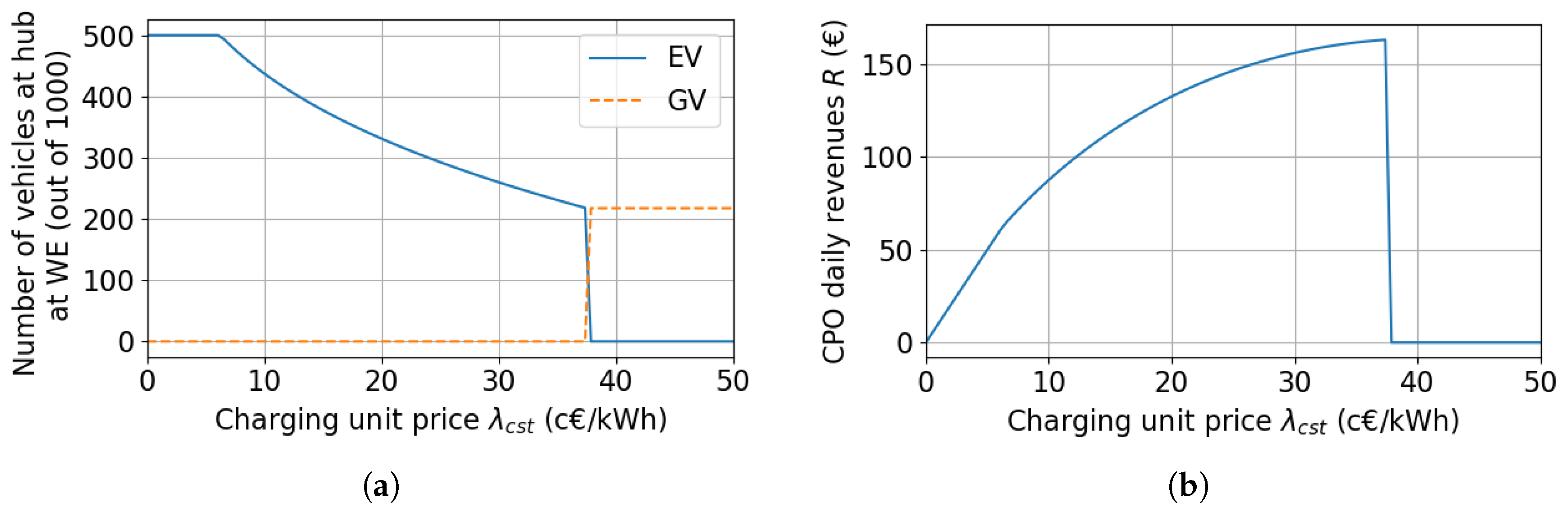
3.1. Wardrop Equilibrium Representation

When the charging unit price at the hub ${\lambda }_e$ introduced in the previous section is an increasing function of the total charging need $L_e\left(x_{e,publ}\right)$ (which is the case here), a unique Wardrop equilibrium (WE) exists—please refer to our previous work [13], Corollary 1. This equilibrium corresponds to a situation where no vehicle could lower its cost by choosing the other transport mode. To illustrate the concept of WE, we consider the parameters values set in Section 2.1.2 and no PV production. The WE corresponding to this particular case is $(x_{e,publ}^{*},x_{g,publ}^{*})=(0.53,0)$, meaning that no GV choose the public transport mode while half EV do so. To understand why, the different EV costs are shown in Figure 6 for any proportion $x_{e,publ}$ of EV choosing the public mode, with fixed $x_{g,publ}=x_{g,publ}^{*}$ (at its WE value).

For example, if there were no EV choosing the public transport mode ($x_{e,publ}=0$, on the extreme left of Figure 6), the total cost for EV choosing the private mode would be higher than for those choosing the public one, due to the congestion effect on the travel duration. Thus, $x_{e,publ}=0$ cannot be an equilibrium situation, as some EV would prefer the public mode which is cheaper. Similarly, too many EV at the hub ($x_{e,publ}>0.53$) would lead to $c_{e,publ}>c_{e,priv}$, so that it is not a WE as some EV would rather choose the private transport mode. In turn, Figure 6 shows that there is a unique WE $x_{e,publ}=0.53$. Note that in this case total costs are equal between the two transport modes, so that no EV would rather choose the other mode. In addition, note that the monetary cost for vehicles at the hub (blue dotted line) are made of a fixed part (the ticket fare), and of a variable part (the charging cost) which depends on the proportion $x_{e,publ}$ of EV choosing the public transport mode.

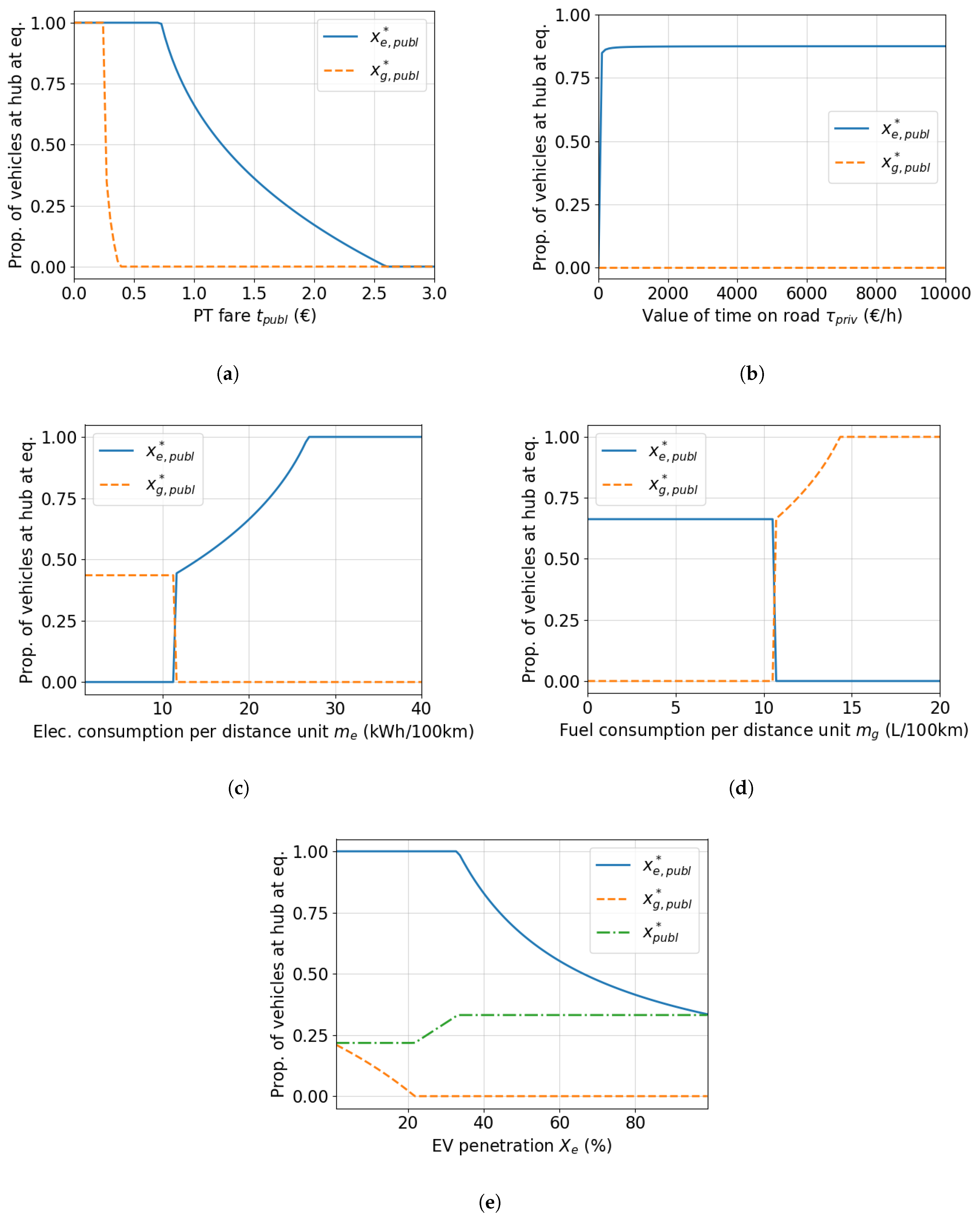
3.2. Equilibrium Sensitivity to Parameters of the Problem

Thanks to the WE obtained in the proposed model, network operators are able to predict the number of EV and GV choosing the public or the private transport modes, whatever the problem parameters may be. In this section, the sensitivity of the WE is studied for various parameters of the problem. The default values of parameters correspond to the ones given in previous section, except that here it is supposed that there is enough PV production so that the charging unit price ${\lambda }_e$ at the hub is reduced to its constant component ${\lambda }_{\mathrm{cst}}$.

Figure 7a shows the proportions of vehicles choosing the public transport mode in function of ticket fare. Starting from the right side of the Figure and decreasing ticket fare from $t_{publ}=3$ €, EV are the first and only ones choosing the public transport mode instead of the private one. This is because EV have more to gain than GV in terms of consumption costs by switching from private to public mode, due to the large amount of PV production available. Some GV will choose the public mode only when all EV will have already chosen the public mode. No vehicle will be left downtown if the ticket fare is under $t_{publ}=0.25$ €. Note that the same sensitivity is obtained with the Public Transport duration $d_{publ}$ or the value of time ${\tau }_{publ}$ in PT.

In Figure 7b, the impact of the value of time ${\tau }_{priv}$ on the road is studied. Note that the ratio $\frac{{\tau }_{publ}}{{\tau }_{priv}}=1.2$ is kept constant, so that the value of ${\tau }_{publ}$ changes too. When the value of time is small, vehicles do not mind if their trip is very time-consuming, so that most vehicles prefer driving in the congested city-center rather than paying a PT ticket.

The WE sensitivity to the consumption of EV per distance unit $m_e$ is showed in Figure 7c. The proportion of EV choosing the public mode is an increasing function of this consumption, as driving into the city-center becomes more expensive. The value $m_e=12$ kWh/100km corresponds to the threshold where EV have more to gain than GV in terms of consumption costs by switching from private to public mode. Similar results are obtained with the consumption of GV per distance unit $m_g$ in Figure 7d.

Finally, Figure 7e shows the proportions of EV and GV at the hub for any proportion of EV $X_e$ among all vehicles. The first new EV (left of figure) will replace the last GV parked at the hub. Then, the additional EV will choose the private transport mode in order to keep the congestion in the city-center balanced with the other financial costs. As there are more and more EV in this problem, the number of vehicles at the hub remains almost constant, so that the proportion of EV choosing the public transport mode necessarily decreases.

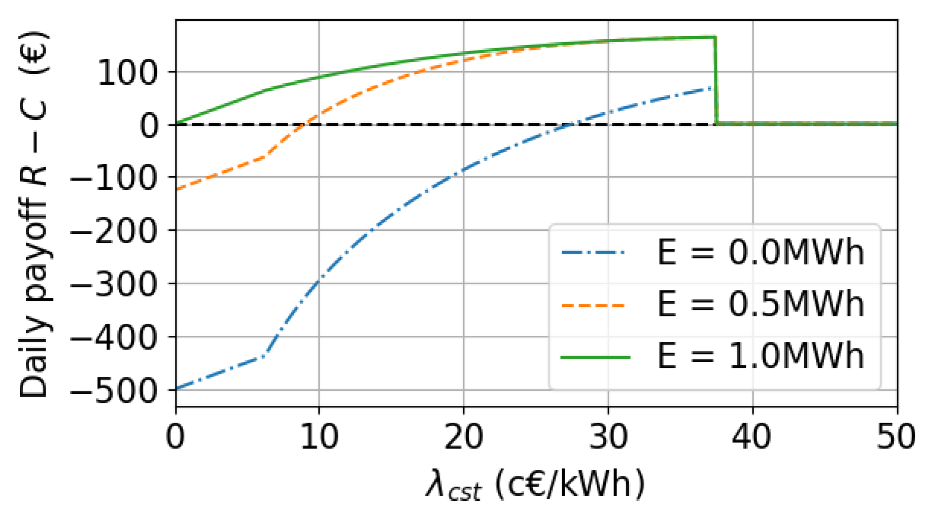
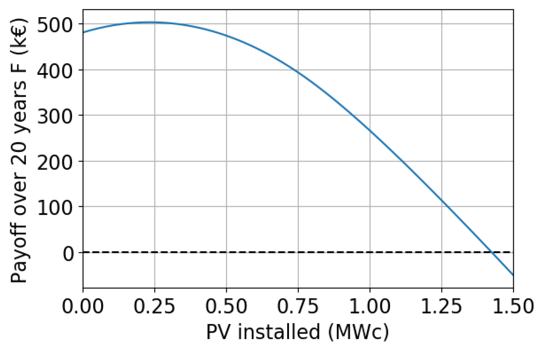
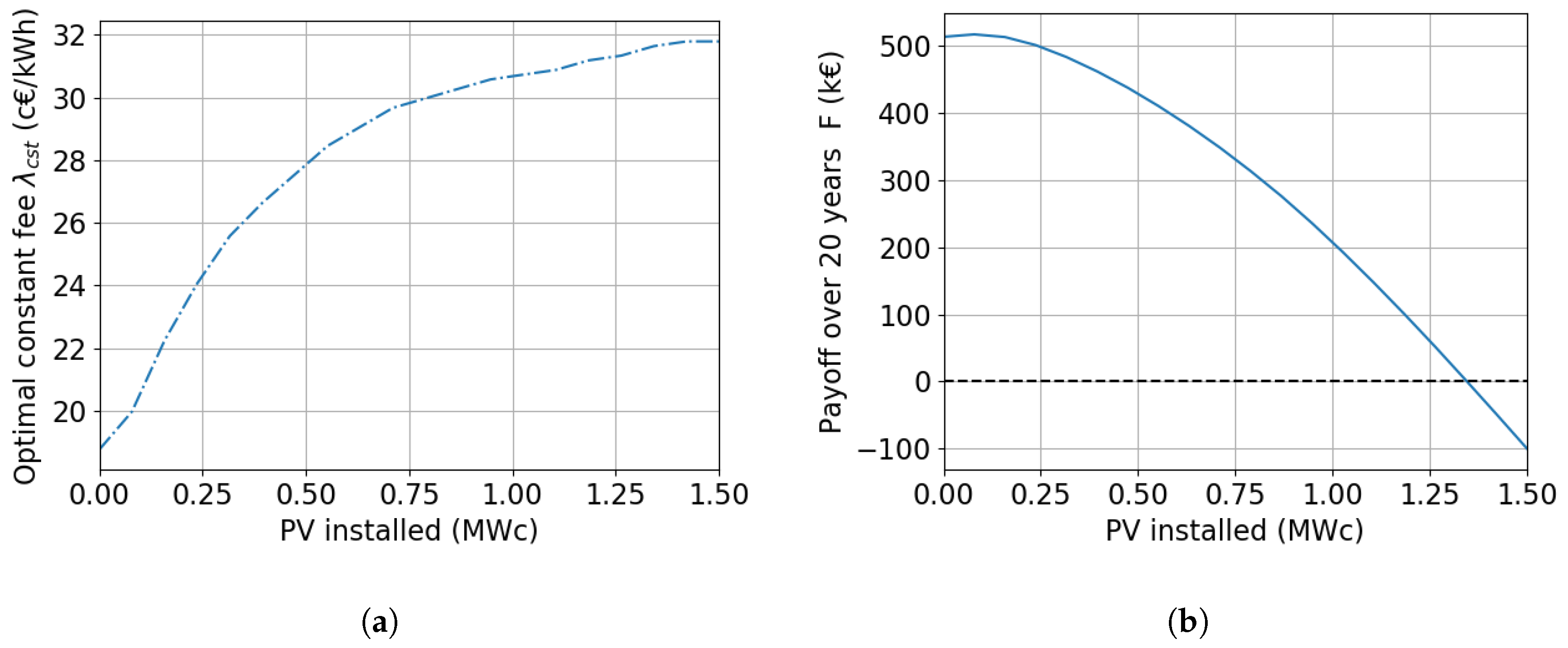
3.3. Optimal Solar Panel Surface

In this section, we focus on the financial viability of investing into PV solar panels at the hub, over a period of time T of interest for the CPO (here, $T=20$ years). The CPO chooses the size of its solar park, and is associated with an objective function F which corresponds to its payoff obtained T years after investing into solar panels. As the CPO is assumed to be in charge of the PV panels, the electrical grid and the EVCS, this payoff F is made of three different parts:

$$F=-I+T\times \sum \left(R-C\right),$$

(10)

with:

• I the initial Investment cost in solar panels, with 750 €/kWp for a solar park of the order of magnitude of 1 MWp,

and, summed over the days of a typical year:

• C the daily grid Costs (associated with the electricity bought from the grid), defined in Equation (8),
• R the daily Revenues from EV charging at the hub which are, by definition of the charging unit price ${\lambda }_e$:

  $$R={\lambda }_e\times L_e\left(x_{e,publ}^{*}\right),$$

  (11)

  with $x_{e,publ}^{*}$ the proportion of EV at the hub at equilibrium corresponding to ${\lambda }_e$ and the total charging need $L_e$, defined in Equation (4).

This section shows that thanks to our model, the CPO can find the optimal PV size which maximizes its payoff F. Note that the goal of this section is not to precisely tackle the PV sizing issue but only to give possible applications of our model.

As a first step, this payoff is studied in the framework introduced in Section 2 except from the charging unit price ${\lambda }_e$ at the hub, whose variable component has been omitted. Hence, ${\lambda }_e={\lambda }_{\mathrm{cst}}$ is constant throughout the period of time T and does not depend on the number of EV charging at the hub $x_{e,publ}$. The full charging unit price ${\lambda }_e$ introduced in Equation (9) is considered afterward.

Before computing the optimal PV size, the CPO has to find for each PV size the optimal ${\lambda }_{\mathrm{cst}}$, the constant charging unit price at the hub for the T years to come, which maximizes F. For the moment, the solar park is fixed to 1MWp for the calculations, corresponding approximately to a surface of 450 parking spots. Figure 8a shows how ${\lambda }_{\mathrm{cst}}$ impacts the number of vehicles at the hub at equilibrium.

For ${\lambda }_{\mathrm{cst}}\le 7$ c€/kWh, charging at the hub is cheap enough so that all EV choose this option while all GV prefer to drive through the empty (from all EV) city center. Naturally, the higher ${\lambda }_{\mathrm{cst}}$, the fewer EV at the hub at equilibrium but the higher the daily revenues R: the decrease in the number of EV at the hub is compensated by the increase in ${\lambda }_{\mathrm{cst}}$ (see Figure 8b). Figure 8a also shows that there is a threshold ${\lambda }_{\mathrm{cst}}^{*}=37.5$ c€/kWh above which charging at the hub is so expensive that all EV would rather drive downtown and some GV would stop at the hub to avoid downtown congestion. This threshold happens to be the optimal charging unit price which maximizes the daily revenues R (see Figure 8b).

Note that the equilibrium illustrated in Figure 8a is the same for any daily PV energy E produced at the hub, since in this simplified framework the charging unit price ${\lambda }_{\mathrm{cst}}$ does not depend on charging demand and PV production (unlike ${\lambda }_e$ defined in (9)). While the revenues R illustrated in Figure 8b do not depend on E either, the electricity distribution cost C does depend on the amount of electricity taken from the grid, and thus on E. Figure 9 shows the daily payoff $R-C$ in function of the charging unit price ${\lambda }_{\mathrm{cst}}$ at the hub, for different daily PV productions E. Note that for $E\ge 1$ MWh, there is enough PV production for all EV so that there are no grid costs and maximizing the payoff is equivalent to maximizing the revenues R (the top curve in Figure 9 is the same as Figure 8b).

Figure 9 illustrates the fact that the threshold ${\lambda }_{\mathrm{cst}}^{*}=37.5$ c€/kWh maximizes the daily payoff $R-C$, no matter the PV production E (e.g., for all PV sizes and any day of the year). This means that choosing the same ${\lambda }_{\mathrm{cst}}={\lambda }_{\mathrm{cst}}^{*}$ for every day of the year is better than any pricing made of a constant charging unit price each day, like for instance peak/off-peak tariffs (e.g., one for winter and one for the rest of the year). Naturally, the maximal payoff increases with E, and is always positive, even for $E=0$. This means that even if EV at the hub may cause grid costs C, the payoff $R-C$ will always be better than when there are no EV at the hub (i.e., $R-C=0$).

In the following, the solar park is not fixed to 1 MWp any longer: in Figure 10 the payoff F over 20 years (with ${\lambda }_{\mathrm{cst}}={\lambda }_{\mathrm{cst}}^{*}$) is represented in function of the PV nominal power.

Figure 10 shows that the payoff F is concave, as grid costs C defined in (8) is a quadratic function of the PV nominal power (for daily PV productions low enough), I is linear and R constant. As nominal power increases, revenues R remain the same while investments I increase proportionally and grid costs C decrease to zero. Installing solar panels can be profitable if the investments are lower than the grid costs avoided (as it is the case here), but the solar park must not be oversized or the improvement in grid costs will not be significant enough compared to the investments. In order to maximize its payoff F (around 503 k€), the CPO has to install a 236 kWp solar park, corresponding to a surface of 110 parking spots. The CPO can install up to 1.43 MWp of PV (corresponding to 650 parking spots) until its payoff F becomes negative.

Two key parameters impact the nature of the previous results. First, the period of time T over which the CPO’s payoff is considered: for small enough T, the optimal way to maximize the CPO’s payoff is not to install PV at all. The same phenomenon is observed for low enough charging unit price ${\lambda }_e^0$ inside the city. In these cases, the charging unit price ${\lambda }_{\mathrm{cst}}$ at the hub must be low enough too in order to attract EV at the hub. However, these ${\lambda }_{\mathrm{cst}}$ are too low to have sufficient revenues R to pay back the initial investment in PV I.

The previous study can now be easily extended to the variable charging unit price ${\lambda }_e$ introduced in Equation (9). As in the previous simplified framework, the CPO has to choose the optimal fixed part ${\lambda }_{\mathrm{cst}}$ of ${\lambda }_e$ for all PV nominal power values. Note that here, unlike in the simplified framework, the optimal ${\lambda }_{\mathrm{cst}}$ depends on the nominal power (see Figure 11a): larger PV capacities lead to lower grid costs and thus lower ${\lambda }_e$ due to the variable part, so that the CPO may increase the fixed part ${\lambda }_{\mathrm{cst}}$ in compensation. After 20 years, the payoff F is similar to the one of the simplified framework (see Figure 11b compared to Figure 10), although the maximal payoff (reached with a 89 kWp solar park, equivalent to surface of 40 parking spots) is 3 % higher with the charging unit price ${\lambda }_e$ defined in Equation (9). This means that a real-time feedback on the impact of the charging operation on the grid for EV owners (i.e., the variable part of ${\lambda }_e$) yields higher revenues for the CPO.

4. Conclusions

This work focuses on the following scenario: electric and gasoline vehicles (EV and GV) can either drive all the way from the suburbs to the city center, or stop at an e-Park & Ride hub and continue by public transport. At the hub, a charge point operator (CPO) is in charge of the charging scheduling in presence of a local PV production. The vehicles’ choices are predicted taking into account congestion effects both on the traffic and on the electrical grid. The latter is represented here as a quadratic cost depending on the net curve at the charging station. Then, predictions of drivers’ reaction to various control parameters can be made. For example, using real data of PV production, the CPO can compute the PV surface which maximizes its profits by inciting EV to stop and charge at the hub. Similarly, the public transport operator can compute the optimal ticket fare, to attract vehicles at the hub and minimize congestion and local pollution in the city center. In a future work, each EV will have the possibility to choose its own charging need and charging place based on its initial State of Charge (instead of being fully charged). In addition, the case when the charging station is located on a site with other non-controlled electricity consumptions could be considered. In this case, the local PV production has to be shared between the charging usage and the other ones.

References

1. Réseau de Transport d’Électricité. Bilan prévisionnel de l’équilibre offre-demande d’électricité en France - Édition 2017; Technical Report; RTE: Donnybrook, Ireland, 2018. (In French) [Google Scholar]
2. Jacquot, P.; Beaude, O.; Gaubert, S.; Oudjane, N. Analysis and Implementation of an Hourly Billing Mechanism for Demand Response Management. IEEE Trans. Smart Grid 2018, 10, 4265–4278. [Google Scholar] [CrossRef]
3. Beaude, O.; Lasaulce, S.; Hennebel, M.; Mohand, I. Reducing the Impact of EV Charging Operations on the Distribution Network. IEEE Trans. Smart Grid 2016, 7, 2666–2679. [Google Scholar] [CrossRef]
4. Brenna, M.; Falvo, M.; Foiadelli, F.; Martirano, L.; Massaro, F.; Poli, D.; Vaccaro, A. Challenges in energy systems for the smart-cities of the future. In Proceedings of the 2012 IEEE International Energy Conference and Exhibition, Florence, Italy, 9–12 September 2012; pp. 755–762. [Google Scholar]
5. Tan, J.; Wang, L. Real-time charging navigation of electric vehicles to fast charging stations: A hierarchical game approach. IEEE Trans. Smart Grid 2017, 8, 846–856. [Google Scholar] [CrossRef]
6. Wei, W.; Mei, S.; Wu, L.; Shahidehpour, M.; Fang, Y. Optimal traffic-power flow in urban electrified transportation networks. IEEE Trans. Smart Grid 2017, 8, 84–95. [Google Scholar] [CrossRef]
7. Sheffi, Y. Urban Transportation Networks: Equilibrium Analysis with Mathematical Programming Methods; Prentice-Hall, Inc.: Upper Saddle River, NJ, USA, 1985. [Google Scholar]
8. Jiang, N.; Xie, C. Computing and analysing mixed equilibrium network flows with gasoline and electric vehicles. Comput. Aided Civ. Infra. Eng. 2014, 29, 626–641. [Google Scholar]
9. Altman, E.; Kameda, H. Equilibria for Multiclass Routing Problems in Multi-Agent Networks. Dyn. Games Appl. 2005, 7, 343–367. [Google Scholar]
10. Mohsenian-Rad, A.H.; Wong, V.W.; Jatskevich, J.; Schober, R.; Leon-Garcia, A. Autonomous demand-side management based on game-theoretic energy consumption scheduling for the future smart grid. IEEE Trans. Smart Grid 2010, 1, 320–331. [Google Scholar] [CrossRef]
11. Alizadeh, M.; Wai, H.; Chowdhury, M.; Goldsmith, A.; Scaglione, A.; Javidi, T. Optimal Pricing to Manage Electric Vehicles in Coupled Power and Transportation Networks. IEEE Trans. Control Netw. Syst. 2017, 4, 863–875. [Google Scholar] [CrossRef]
12. Wei, W.; Wu, L.; Wang, J.; Mei, S. Network Equilibrium of Coupled Transportation and Power Distribution Systems. IEEE Trans. Smart Grid 2018, 9, 6764–6779. [Google Scholar] [CrossRef]
13. Sohet, B.; Beaude, O.; Hayel, Y. Routing game with nonseparable costs for EV driving and charging incentive design. In NETwork Games Control and Optimization; Birkhäuser: New York, NY, USA, 2018. [Google Scholar]
14. Spiess, H. Technical note—Conical volume-delay functions. Transp. Sci. 1990, 24, 153–158. [Google Scholar] [CrossRef]
15. Sétra. Fonctions Temps-débit sur les Autoroutes Interurbaines—Détermination du Coefficient D’équivalence et de la Capacité à Partir des Observations Locales. 2001. Available online: http://dtrf.setra.fr/pdf/pj/Dtrf/0002/Dtrf-0002996/DT2996.pdf?openerPage=notice (accessed on 30 October 2019).
16. Fontana, M.W. Optimal Routes for Electric Vehicles Facing Uncertainty, Congestion, and Energy Constraints. Ph.D. Thesis, Massachusetts Institute of Technology, Cambridge, MA, USA, 2013. [Google Scholar]
17. Wardrop, J. Some theoretical aspects of road traffic research. Proc. Inst. Civ. Eng. Part II 1952, 1, 325–378. [Google Scholar] [CrossRef]
18. Jacquot, P.; Beaude, O.; Benchimol, P.; Gaubert, S.; Oudjane, N. A Privacy-preserving Disaggregation Algorithm for Non-intrusive Management of Flexible Energy. arXiv 2019, arXiv:1903.03053. [Google Scholar]
19. Pfenninger, S.; Staffell, I. Long-term patterns of European PV output using 30 years of validated hourly reanalysis and satellite data. Energy 2016, 114, 1251–1265. [Google Scholar] [CrossRef] [Green Version]
Figure 1. Schematic representation of the charging hub scenario: commuters can either choose to leave their vehicle at the hub and take public transport ( p u b l ), or drive all the way to their destination ( p r i v ). A local source of renewable energy is available at the hub.
Wevj 10 00070 g001
Figure 2. Travel duration d p r i v ( . ) (and the associated cost τ p r i v d p r i v ( . ) , along the right axis) for vehicles driving downtown depending on their proportion x p r i v . If all vehicles choose the private transport mode, the associated duration will be three times higher than the free-flow case (when all vehicles choose public mode).
Wevj 10 00070 g002
Figure 3. Energy produced by 1 m 2 (equivalent to a nominal power of 175 Wp) of a solar panel in Paris during working hours (averaged over the year 2014).
Wevj 10 00070 g003
Figure 4. Cost/impact on the electrical grid of electric vehicles (EV) charging and PhotoVoltai (PV) production (through the net load t ) at time slot t. If PV production is higher (resp. smaller) than EV charging load, there is no (resp. a quadratic) impact.
Wevj 10 00070 g004
Figure 5. Water-filling optimal scheduling of the charging operation with 125 m 2 of solar panel (in black), for 15 EV (in red) and 45 EV (in blue). For 15 EV, any scheduling using only PV production is optimal, while for 45 EV, the only optimal scheduling uses the whole PV production plus the same amount from the electrical grid at each time slot.
Wevj 10 00070 g005
Figure 6. EV costs as a function of the proportion x e , p u b l of EV choosing public transport. In blue (resp. red) is the cost for EV choosing public (resp. private) transport mode. The dotted lines refer to the monetary costs (consumption and ticket fare for public mode; only consumption for private mode) and the dashed lines refer to travel duration. The equilibrium (black star) happens when total costs are equal between the two transport modes, for x e , p u b l = x e , p u b l * = 0.53 .
Wevj 10 00070 g006
Figure 7. Proportion of vehicles at the hub at WE in function of … (a) PT ticket fare t p u b l ; (b) value of time on the road τ p r i v ; (c) unit consumption of EV m e ; (d) unit consumption of GV m g ; (e) penetration of EV X e .
Wevj 10 00070 g007
Figure 8. Impact of the charging unit price λ cst on the Wardrop equilibrium (WE) and the charge point operator (CPO) revenues R. (a) Number of vehicles at the hub at WE in function of λ cst ; (b) CPO daily revenues R in function of λ cst . As λ cst increases, fewer EV choose the hub while R increases, up to a threshold λ cst * = 37.5 c€/kWh beyond which all EV drive downtown.
Wevj 10 00070 g008
Figure 9. Daily payoff R C in function of the charging unit price λ cst at the hub, for different daily PV productions E. No matter E, λ cst = λ cst * maximizes R C .
Wevj 10 00070 g009
Figure 10. Payoff F over 20 years (with λ cst = λ cst * ) in function of the PV nominal power. The CPO can make more profits by installing (the right amount of) PV.
Wevj 10 00070 g010
Figure 11. Optimal CPO variables to maximize F in function of nominal power. (a) Optimal fixed part λ cst * ) in function of nominal power; (b) Payoff F (with λ cst = λ cst * ) in function of nominal power. The variable charging unit price λ e offers a little more benefit than a fixed one ( λ cst , Figure 10).
Wevj 10 00070 g011