Article

Hierarchical Coordinated Control Method of In-Wheel Motor Drive Electric Vehicle Based on Energy Optimization

School of Mechanical Engineering, Anyang Institute of Technology, West Section of Yellow River Avenue, Anyang City 455000, China
*
Author to whom correspondence should be addressed.
World Electr. Veh. J. 2019, 10(2), 15; https://doi.org/10.3390/wevj10020015
Submission received: 21 January 2019 / Revised: 15 March 2019 / Accepted: 29 March 2019 / Published: 1 April 2019

Abstract

:
In order to improve the endurance mileage and stability of an electric vehicle at the same time, a hierarchical coordinated control method of an in-wheel motor drive electric vehicle based on energy optimization is presented in this paper. The driving architecture of an in-wheel motor drive electric vehicle is developed, and a corresponding simulation model is established in CarSim software; then, the bicycle model of an electric vehicle is derived from vehicle dynamic equations. The energy-saving feasibility of an in-wheel motor drive electric vehicle is analyzed by a motor efficiency map, and on the basis of this, the hierarchical coordinated control method is proposed to achieve the simultaneous energy optimization control and stability control of the electric vehicle. The results show that the energy consumption is decreased by 32.41%, 45.92%, and 4.07% in different simulation manoeuver cases, and the vehicle stability can be ensured by the proposed control method.

1. Introduction

With the rapid development of automobile industry technology and the improvement of people’s living standards, the production capacity, sales, and per-capita share of the automobile market are also increasing year by year [1,2,3]. In today’s world, economic development and scientific and technological progress are undeniable mainstream value requirements and social development trends, but at the same time, the shortage of energy and environmental pollution problems are a point they can never ignore. With the aggravation of the global greenhouse effect, public opinion around the world has given more stringent expectations and standards on how to reduce vehicle emissions. How to break through the restrictions of energy shortage and environmental pollution, and how to mitigate the increasingly severe greenhouse effect, has become one of the key issues that cannot be ignored in the automotive industry [4,5,6].
The most prominent advantage of electric vehicles is that they can reduce emissions or even achieve zero emissions [7,8,9]. At the same time, the electricity that they need is renewable energy. The development of electric vehicles will help alleviate a series of problems such as energy shortage, environmental pollution, and even greenhouse effects. Wang et al. [10] designed a novel optimal torque distribution method and applied it to the longitudinal motion control of an in-wheel motor drive electric vehicle with the load transfer being considered, and the simulation and experimental result validate that the vehicle energy efficiency has been improved. Chen et al. [11] proposed a whole energy control strategy according to the motor efficiency and traffic model, and obtained the global optimal vehicle speed requirement and driving torque distribution results to minimize the overall energy consumption. In recent years, electric vehicle batteries represented by lithium batteries have also ushered in explosive development, and the corresponding driving motor technology and automotive electronic control technology are becoming increasingly perfected and market-oriented, which also provides a better possibility for the rapid development of electric vehicles [12,13,14]. In this context, endurance mileage has become one of the most important factors restricting the popularity of electric vehicles, so it is necessary to study the energy optimization of electric vehicles.
The in-wheel motor drive electric vehicle is a relatively new structure in the field of electric vehicles, which can be directly driven by four in-wheel motors. The driving torque of an in-wheel motor can be operated independently and has a shorter response time and higher precision than standard motors, which can provide the basis for the accurate electric drive control of the whole vehicle in real time, and provide more possibilities and freedom for active safety control [15,16,17], stability control [18,19,20,21], and real-time torque control for energy-saving purposes [22,23,24]. Nam et al. [20] developed a lateral tire force sensors-based electric vehicle sideslip angle control strategy, in which extended Kalman filtering was designed to estimate vehicle running states and provide the inputs to the vehicle lateral stability controller. Chen et al. [23] presented an adaptive energy optimization control distribution method to make distributed control actuation gradually converge to energy-optimal operating points by solving nonlinear optimization problems. Dizqah et al. [24] proposed a driving torque optimal allocation method using a solution method for a vehicle speed-based parameter optimization problem; experiments have been carried out, and the energy-saving effect has been confirmed. Observing the existing literature, we can see that most of the literature investigates vehicle stability control and vehicle energy optimization control through directional tire force distribution. There are few studies on the coordinated control of vehicle stability improvement and vehicle energy optimization. If the driving characteristics of an in-wheel motor drive electric vehicle are fully utilized and the corresponding coordinated control strategy is designed, the vehicle stability can be well ensured, and the energy utilization rate of the vehicle can be improved at the same time.
In this paper, motivated by the above analysis, a hierarchical coordinated control method of an in-wheel motor drive electric vehicle based on energy optimization is proposed. The driving architecture of an in-wheel motor drive electric vehicle is designed, and the corresponding simulation model in CarSim software and the bicycle model of an electric vehicle are established for the basis of this work. The analysis of energy-saving feasibility is carried out according to the motor efficiency map, and the hierarchical coordinated control method is finally designed to achieve the energy optimization control and vehicle stability control, which has certain theoretical research significance and engineering application value.
The rest of this paper is organized as follows. The driving architecture and dynamic model of an electric vehicle are presented in Section 2. The energy-saving feasibility of an in-wheel motor drive electric vehicle is analyzed in Section 3. The hierarchical coordinated control method based on energy optimization is designed in Section 4. The simulation results are provided in Section 5, and the conclusive remarks are presented in Section 6.

2. Driving Architecture and Dynamic Model of an Electric Vehicle

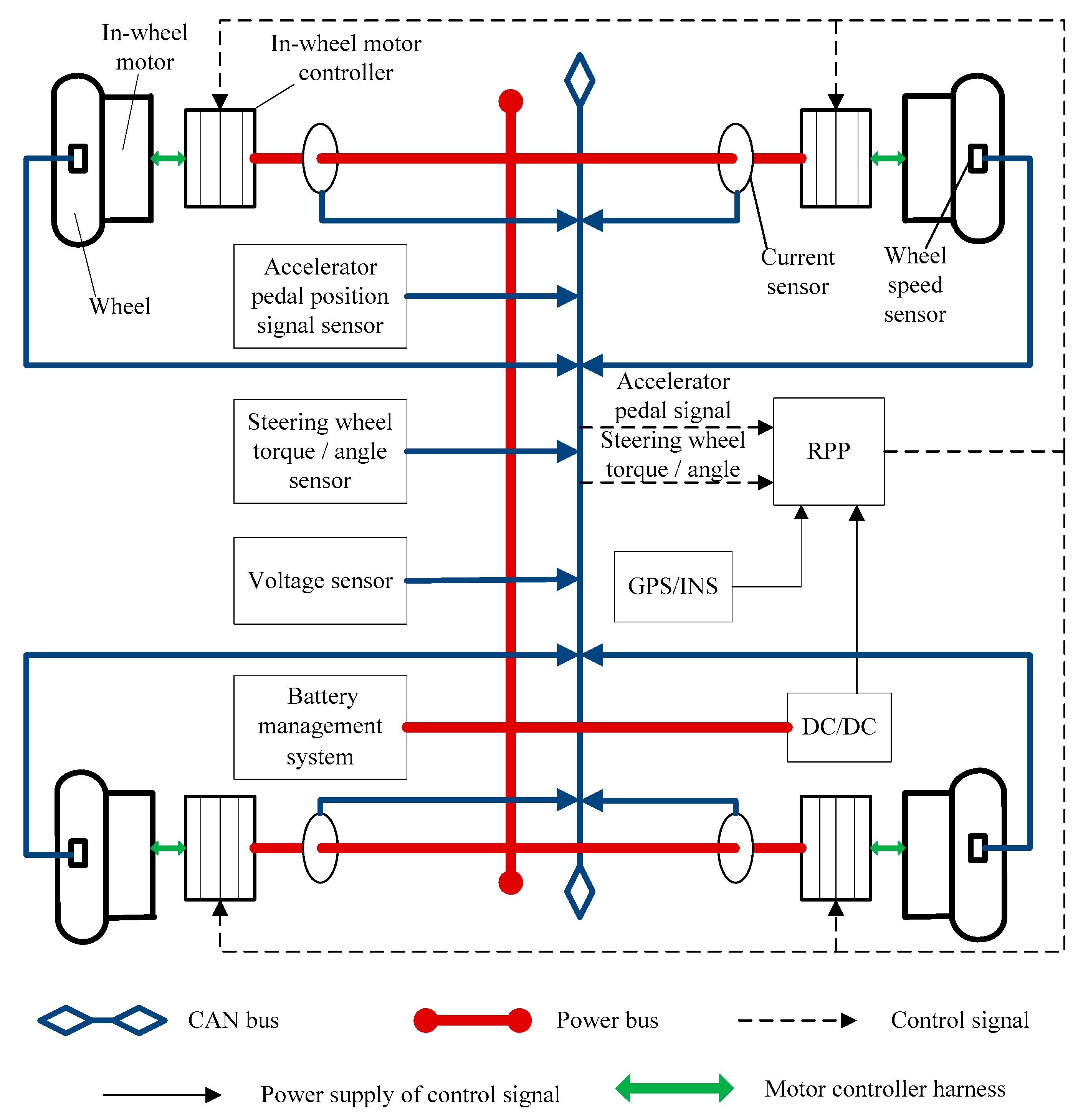
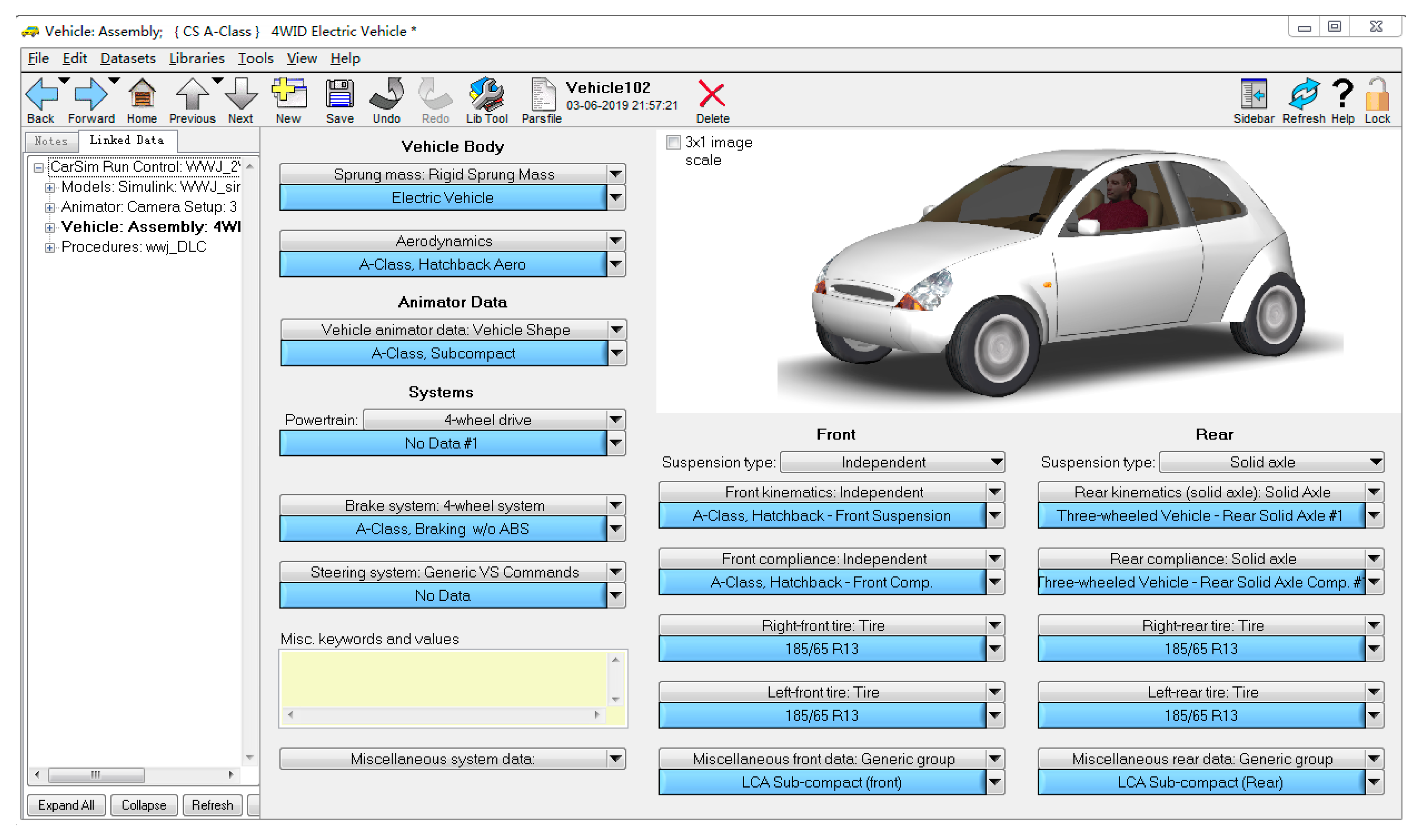
2.1. Driving Architecture and Simulation Modeling

In order to facilitate the study of all the vehicle characteristics of a four-wheel independent drive electric vehicle, a four-wheel independent drive test prototype vehicle was designed based on a pure electric vehicle, and its driving architecture is shown in Figure 1. In order to realize four-wheel independent driving, four in-wheel motors are installed at each wheel of the test prototype vehicle as driving motors. Considering the factors of power density, volume, weight, and price, a permanent magnet brushless DC motor is selected as the in-wheel motor. In order to realize the dynamic control of the whole four-wheel independent drive electric vehicle, the rapid prototyping platform (RPP) is used to build the vehicle controller network and its electronic and electrical architecture. The vehicle is equipped with a high-precision global positioning system (GPS) and inertial navigation system (INS) to measure the cruising trajectory and body posture of the vehicle. In addition, the vehicle is equipped with a current sensor, wheel speed sensor, and voltage sensor to record the status of the in-wheel motors.
CarSim is the common and convenient vehicle dynamics simulation software, and its computing power is more than three to six times faster than the actual situation. It can be used to realize the simulation analysis of vehicle response to the driver, road surface, and aerodynamic input. It can be used to achieve a simulation analysis of important indexes in vehicle handling stability, ride comfort, dynamic property, braking performance, and economy. CarSim software can define the simulation environment and simulation process according to the needs of developers, and can set the simulation parameters and characteristic files of vehicle control systems by itself. The existing vehicle dynamics simulation models in CarSim software are designed for traditional internal combustion engine vehicles, and the distributed drive electric vehicle model that we need to build is driven directly by in-wheel motors, which means that the original default engine, gearbox, differential, and other transmission systems in the CarSim model need to be deleted, as shown in Figure 2. According to the vehicle parameters in Table 1, the dynamic model of the whole distributed drive electric vehicle is built. At the same time, the drive torque output model of an in-wheel motor is built to replace the original transmission system and realize the real distributed drive electric vehicle modeling.

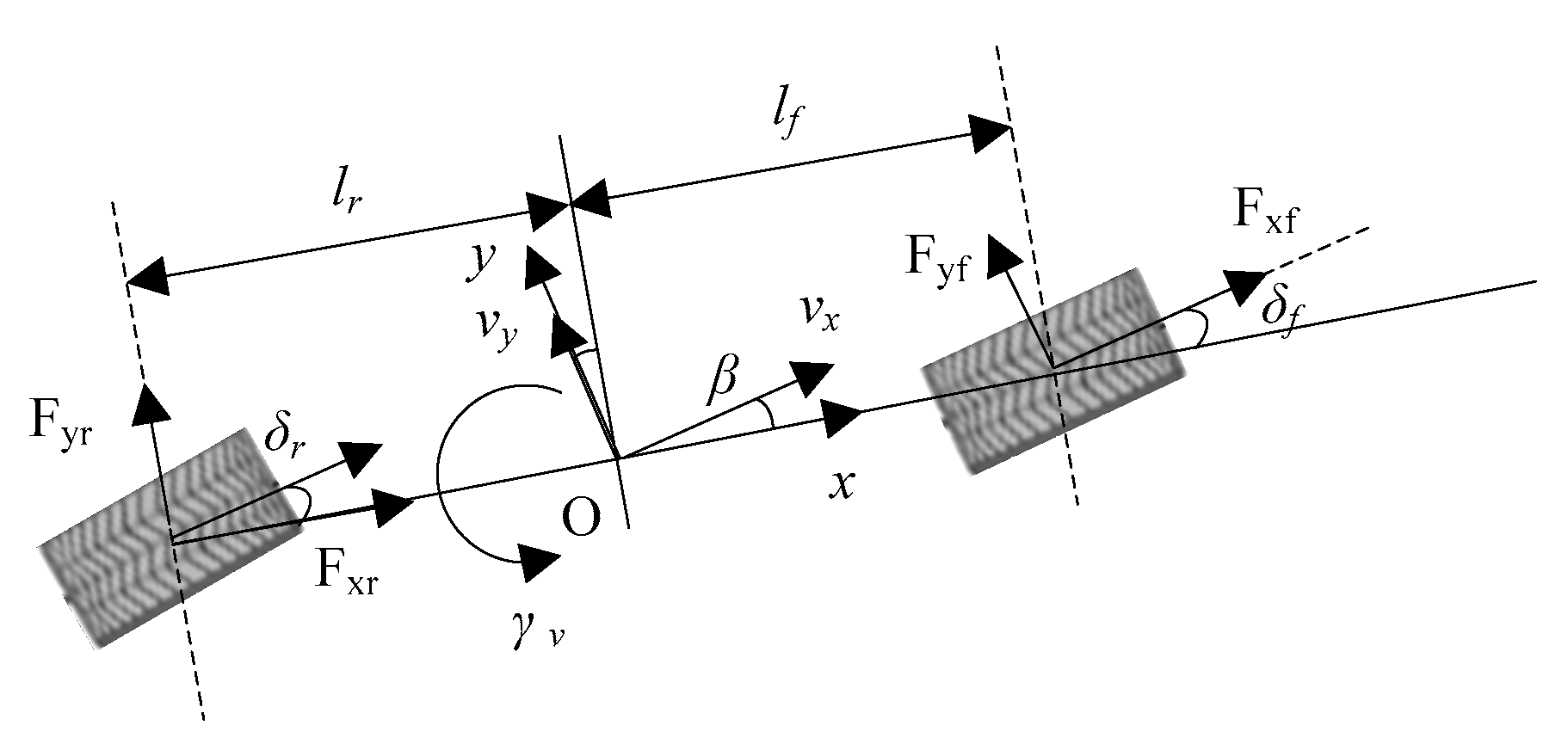
2.2. Vehicle Dynamic Model

A bicycle model is established to characterize vehicle dynamics behavior in lateral and yaw-direction motions. The origin of the dynamic coordinate system XY is fixed on the vehicle and coincides with the center of gravity of the vehicle. The X-axis represents the longitudinal axle of the vehicle, and the Y-axis represents the horizontal axle of the vehicle. It is assumed that the mechanical properties of each tire are the same. The schematic diagram of the vehicle dynamic model is shown in Figure 3, and the vehicle dynamics equation is expressed as:
m v x β ˙ = F y f + F y r m v x γ ,
I z γ ˙ = l f F y f l r F y r + Δ M z ,
where vx represents the longitudinal vehicle speed, γ is the yaw rate of the vehicle, m is the vehicle mass, β denotes the vehicle sideslip angle, Iz stands for the moment of inertia, lf and lr are the distances from vehicle gravity center to the front and rear axle, respectively, and Fyf and Fyr are the generalized front and rear lateral forces, respectively, i.e., Fyf = Fy1 + Fy2, Fyr = Fy3 + Fy4. Δ M z is the external yaw moment generated by four in-wheel motors, which can be expressed as:
Δ M z = ( F x 2 F x 1 ) b f cos δ + ( F x 1 + F x 2 ) l f sin δ + ( F x 4 F x 3 ) b r ,
where bf,r is the half tread of the wheel base, δ is the steering angle of the front wheels, Fxj (j = 1, 2, 3, 4) represents the longitudinal force of the ith tire. Assuming that the steering angle of the front wheel is small and the tire operates in a linear area, Fyf and Fyr can be given by:
F y f = 2 C f α f F y r = 2 C r α r ,
where Cf expresses the cornering stiffness of the front tires, Cr expresses the cornering stiffness of the rear tires, αf represents the slip angle of the front tires, αr represents the slip angle of the rear tires, and the tire slip angle can be obtained as:
α f = δ f l f γ / v x β α r = l r γ / v x β ,
According to the above equations, the vehicle dynamic model is written as:
β ˙ = C f + C r m v x 2 β ( 1 + C f l f C r l r m v x 2 ) γ + C f m v x δ f ,  
γ ˙ = C r l r C f l f I z β C f l f 2 + C r l r 2 I z v x γ + C f l f I z δ f + 1 I z Δ M z ,

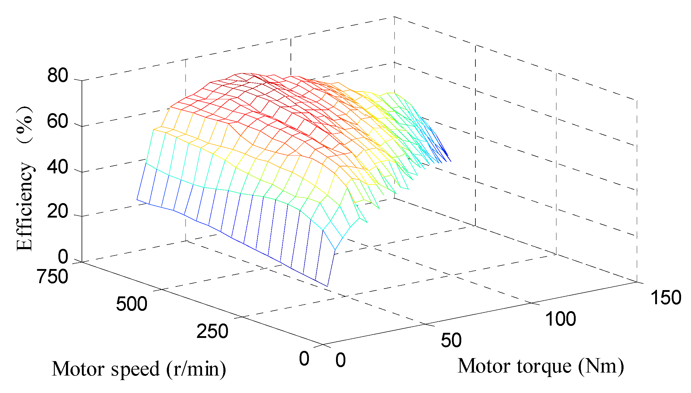
3. Analysis of Energy-Saving Feasibility

The drive efficiency characteristics of in-wheel motors installed on distributed drive electric vehicles are one of the important bases for optimizing the torque distribution results to achieve the energy-saving purpose of distributed drive electric vehicles. In order to obtain the driving efficiency characteristics of an in-wheel motor, the experimental data collected from the bench test of an in-wheel motor were analyzed in Matlab, and the motor efficiency under different torque/speeds was calculated with different motor control signals being given. The efficiency map of an in-wheel motor is drawn, as shown in Figure 4. Figure 4 shows that the real-time efficiency of the motor is different when the torque and speed are different. At the same speed, the influence caused by the change of motor speed on motor efficiency is relatively small, while at the same speed, the influence caused by the change of motor torque on motor efficiency is more obvious. According to the distribution law of motor efficiency, the motor efficiency is relatively low when the torque is large or small, and higher in the middle of the torque. Thus, the principle of the energy-saving torque optimization distribution method of distributed drive electric vehicles is described as: by reasonably distributing the torque of the driving motor, the torque of the driving motor can avoid becoming too large or too small, and work at the higher-efficiency working point as far as possible. Under normal working conditions, it is considered that the torque of the left and right wheels is equal, so the energy-saving torque optimization distribution can be approximated as the problem of torque allocation between the front and rear axles.
The in-wheel motors installed on distributed drive electric vehicles are of the same type; therefore, it can be concluded that the driving efficiency characteristics of the four in-wheel motors are basically the same. Referring to the control network system of a distributed drive electric vehicle, the real-time distribution of the driving torque of four in-wheel motors can be achieved by changing the control signal voltage of the motor controller. A reasonable real-time distribution of the driving motor’s torque according to the driving torque requirement can make the in-wheel motor work as efficiently as possible under the current driving demand, so as to improve the driving efficiency and reduce the vehicle’s energy consumption.

4. Hierarchical Coordinated Control Method Based on Energy Optimization

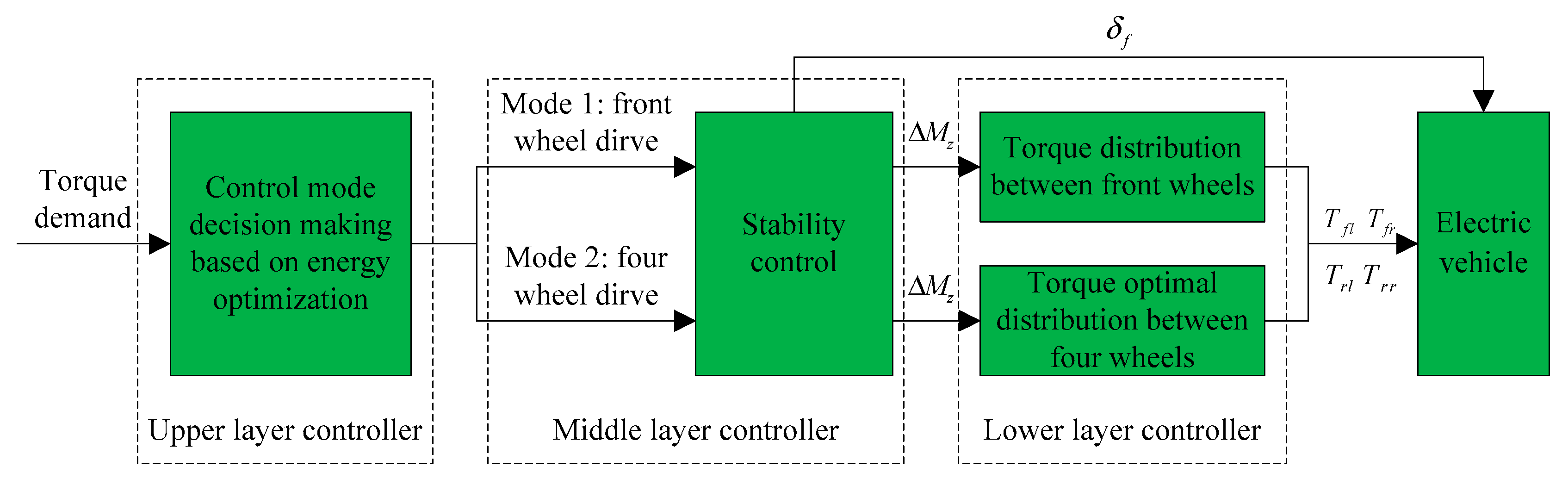
4.1. Overall Control Strategy

The proposed overall control strategy is shown in Figure 5. The hierarchical control method is designed, including an upper layer controller, a middle layer controller, and a lower layer controller. The upper layer controller is used to decide the control mode based on energy optimization. The driving mode 1 is front-wheel drive, and the driving mode 2 is four-wheel independent drive. In the middle layer controller, a vehicle stability controller is presented using a sliding mode controller. The vehicle stability controller in the middle layer will produce the required steering angle of the front wheel and an additional yaw moment, the required steering angle of the front wheel is directly fed into the electric vehicle, and the required additional yaw moment is used as the input of the lower layer controller. In the lower layer controller, different torque distribution methods are designed according to different driving modes. If mode 1 is chosen, the differential torque distribution method between the front wheels is applied, and if mode 2 is chosen, the optimal torque distribution method between the four wheels is applied.

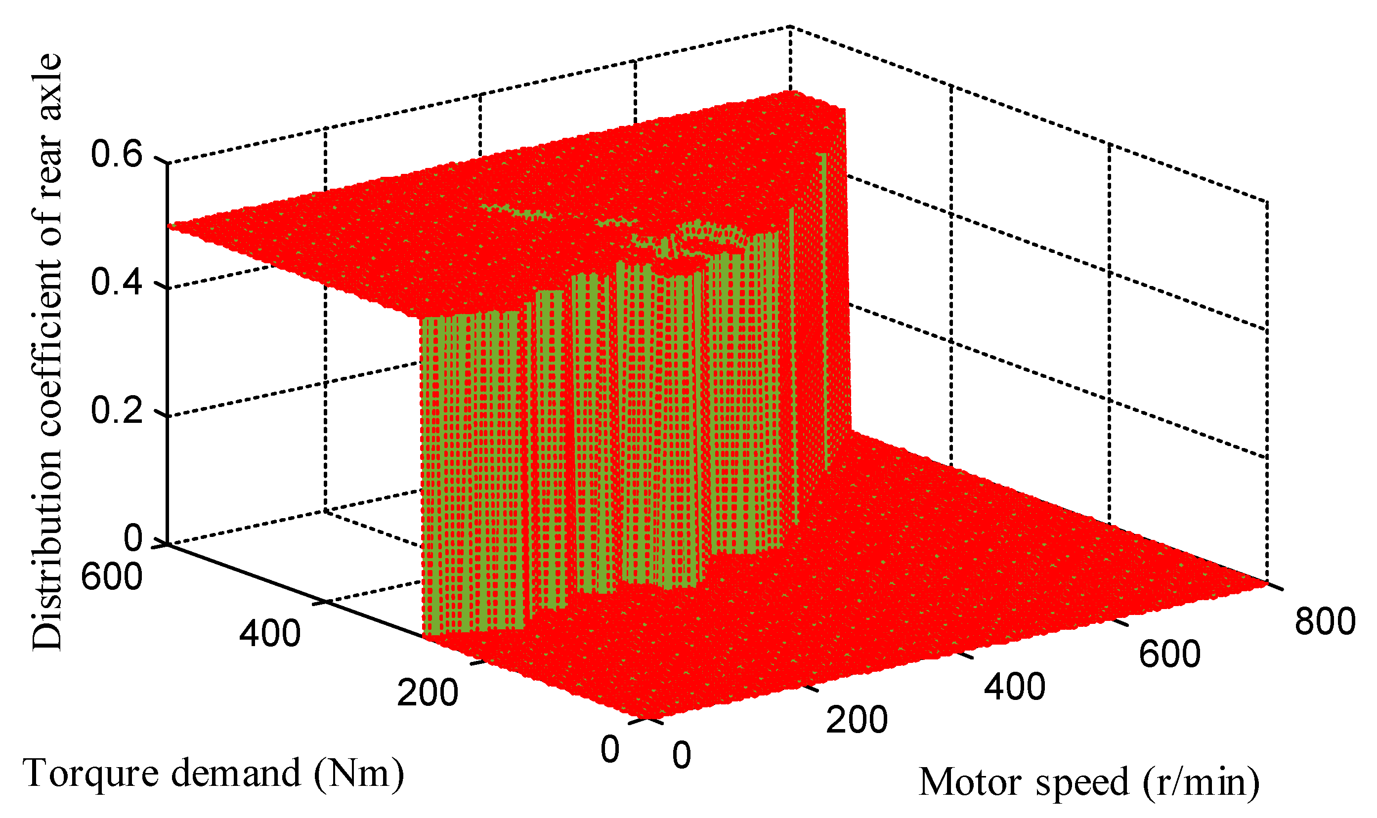
4.2. Upper Layer Controller: Driving Mode Decision

Under the same driving conditions, the vehicle has the same torque demand and speed: that is, the same output power. If the efficiency of the motor is improved, the input power is reduced under the same power demand, which has the function of improving the energy utilization rate and saving energy consumption. The objective function for improving the motor efficiency is written as:
J = min T d n T f n η ( T f , n ) + T r n η ( T r , n ) = min T d n ( 1 λ r ) T d n η ( T f , n ) + λ r T d n η ( T r , n ) = min 1 λ f η ( T f , n ) + 1 λ f η ( T r , n ) ,
where Td is the total torque requirement, n is the motor speed, λ r is the torque distribution coefficient of the rear axle, η ( T f , n ) is the motor driving efficiency of the front axle, and η ( T r , n ) is the motor driving efficiency of the rear axle. The constraint condition can be expressed as: 0 ≤ λr ≤ 0.5, 0 ≤ 0.5λrTdTmax, and 0 ≤ 0.5(1 − λr)TdTmax, where Tmax represents the maximum motor torque. It can be found that when the result of torque optimization is single-axle drive, the front-axle drive is adopted by default, which contributes to the design of vehicle stability control, and the related methods will be introduced in the next section.
The optimization problem is equivalent to solving the nonlinear constrained global optimization problem, so as to obtain the optimal solution. Based on the measured data obtained from the bench test of an in-wheel motor, the optimal rear-axle torque distribution coefficient of the given torque and speed is obtained by offline optimization calculation, as shown in Figure 6. In the real-time control process, the optimal allocation coefficient is obtained by looking up the table according to the current torque and speed using the 2D Lookup Table module in Simulink. From Figure 6, it can be seen that the distributed torque of the front and rear axles is mainly related to the total torque demand. When the demand of the torque is small, the torque distribution coefficient of the front axle is one, which increases the motor torque and makes the working point of the motor approach the high-efficiency area. When the torque demand is large, the torque distribution tends to be average, so as to prevent the reduction of the efficiency caused by the excessive torque of a single motor. Consequently, the driving mode decision can be carried out according to current torque demand and vehicle speed demand.

4.3. Middle Layer Controller: Vehicle Stability Control

According to Equation (6) and Equation (7), the state space equation of a vehicle dynamic model is derived as:
x ˙ = A x + B u ,
where x = [ β γ ] T , u = [ δ Δ M z ] T , A = [ C f + C r m v x 1 l f C f l r C r m v x 2 l r C r l f C f I z l f 2 C f + l r 2 C r v x I z ] , B = [ C f m v x 0 l f C f I z 1 I z ] . Considering the system interference, the state space equation is rewritten as:
x ˙ = A x + B u + d ,
where d is the system interference. Denoting the desired vehicle stability state as [ β d γ d ] T , the stability control error can be expressed as e = [ e β e γ ] T = [ β β d γ γ d ] T , where β d is the desired vehicle sideslip angle, γ d is the desired vehicle yaw rate. The sliding surface of vehicle stability controller is designed as:
s = e + λ e ˙ ,
where s = [ s 1 s 2 ] T , λ = d i a g [ λ 1 λ 2 ] , λ 1 > 0 , λ 2 > 0 .
And the exponential approach law is designed as:
s = η s ξ sgn ( s ) ,
where η = d i a g [ η 1 η 2 ] , η 1 > 0 , and η 2 > 0 ; ξ = d i a g [ ξ 1 ξ 2 ] , ξ 1 > 0 , and ξ 2 > 0 ; and sgn ( s ) = [ sgn ( s 1 ) sgn ( s 2 ) ] T .
The control input of the vehicle stability controller is designed as:
u = B 1 ( λ 1 ( η s ξ sgn ( s ) e ˙ ) + [ β ¨ d γ ¨ d ] ) ,  
In order to prove the stability and convergence of the vehicle stability controller, the Lyapunov function is designed as:
V = 1 2 s T s ,  
Calculating the derivatives of Equation (14), we have:
V ˙ = s T s ˙ = s T ( λ e ¨ ) = s T ( e ˙ + λ [ β ¨ β ¨ d γ ¨ γ ¨ d ] ) ,  
Substituting the control input in Equation (13) into Equation (15), we have:
V ˙ = s T ( η s ξ sgn ( s ) λ d ) s T η s ξ min s + λ d s ,  
where ξ min = min ( ξ 1 , ξ 2 ) . According to Formula (16), it can be found that, with the right choice of controller parameters, the stability condition V 0 can be satisfied.

4.4. Lower Layer Controller: Optimal Torque Distribution Method in Different Driving Modes

In the middle layer controller, the required additional yaw moment is obtained. In this section, the torque distribution method is developed to meet the yaw moment requirement. If the current driving mode is mode 1—that is to say, front wheel drive—the differential torque distribution mean is applied. In this condition, the additional longitudinal forces Δ F x and Δ F x are respectively added to the front-left wheel and front-right wheel to generate the additional yaw moment, and we have:
Δ M z = Δ F b f ,  
If the current driving mode is mode 2, the global optimal torque distribution method is designed. The cost function for meeting the yaw moment requirement is expressed as:
J = F x T W 1 F x J 1 + ( B x F x Δ M z ) T W 2 ( B x F x Δ M z ) J 2 ,  
where B x = [ cos δ f b s + l f sin δ f cos δ f b s + l f sin δ f cos δ f b s + l f sin δ f cos δ f b s + l f sin δ f ] is obtained by Equation (3), F x = [ F x 1 F x 2 F x 3 F x 4 ] T is the distributed longitudinal force, W 1 = d i a g [ m g 4 F z 1 m g 4 F z 2 m g 4 F z 3 m g 4 F z 4 ] is the distribution matrix of J 1 , and W 2 = d i a g [ i = 1 4 F x i 4 F x 1 i = 1 4 F x i 4 F x 2 i = 1 4 F x i 4 F x 3 i = 1 4 F x i 4 F x 4 ] is the distribution matrix of J 2 . The control item J 1 is used to supervise the longitudinal force and make it adaptive to the vertical load. The control item J 2 is used to meet the yaw moment control requirement.
In order to compute the optimal extremum of objective function, solving J F x = 0 , we have:
J F x = W 1 F x + B x T W 2 ( B x F x Δ M z ) = ( W 1 + B x T W 2 B x ) F x B x T W 2 Δ M z = 0 ,  
Then, the distributed tire force is given by:
F x = ( W 1 + B x T W 2 B x ) 1 B x T W 2 Δ M z ,  

5. Simulation Results

In order to verify the control effect of the hierarchical control method proposed in this paper, the simulation verification is carried out in the CarSim Simulink co-simulation platform.

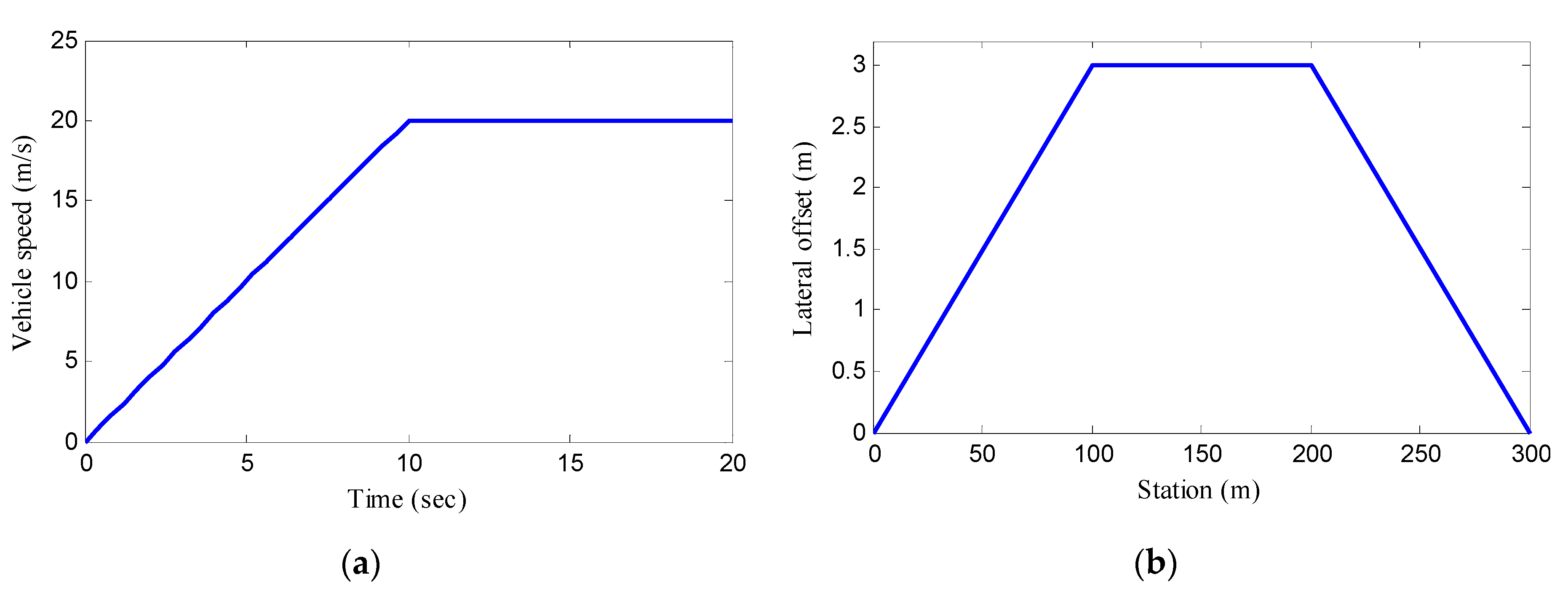
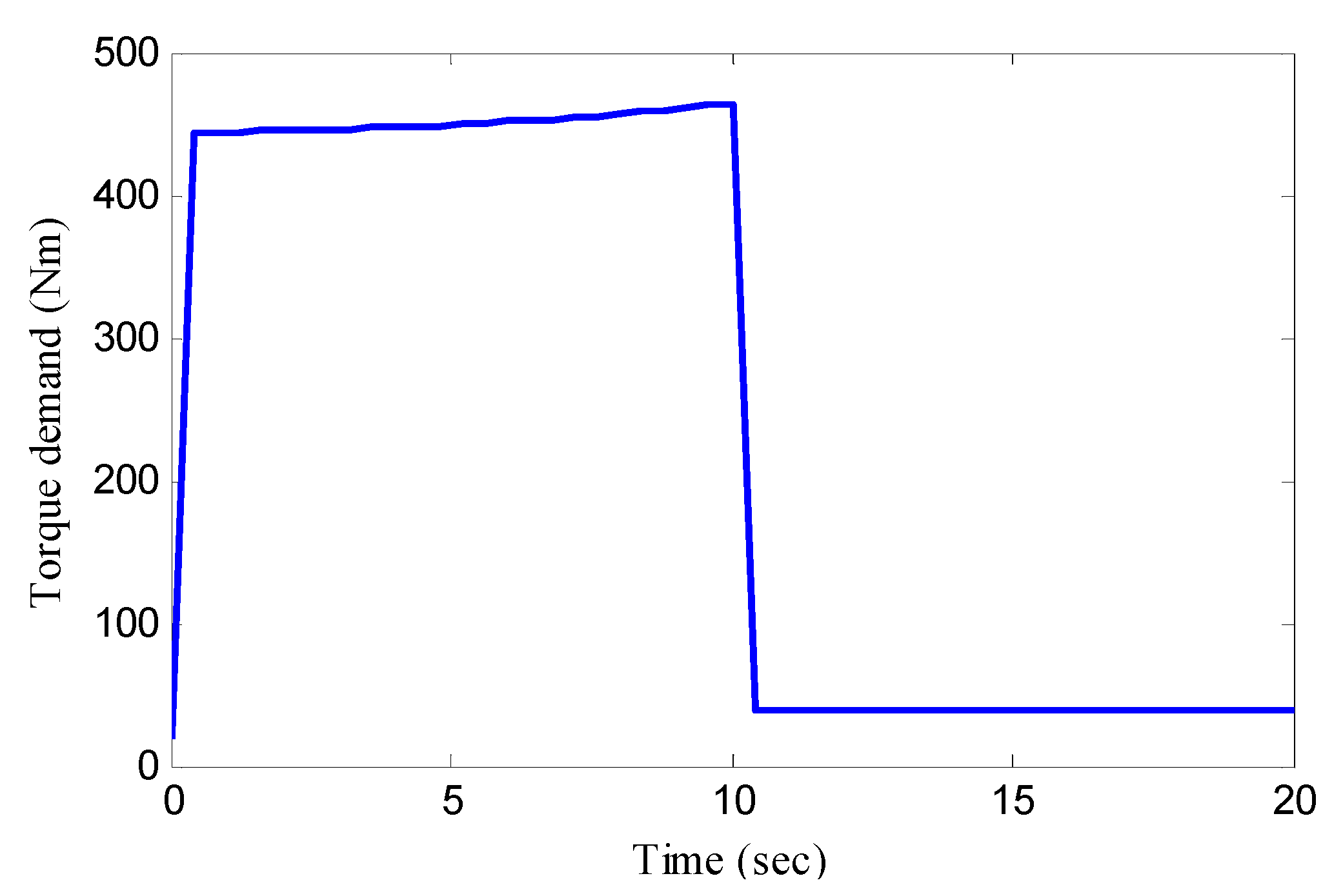
5.1. Double Lane Change Manoeuvre

In case study 1, the simulation condition is shown in Figure 7, including the planned vehicle speed and planned double lane change (DLC) manoeuver trajectory. The road friction coefficient is 1.0 in the simulation. In addition, in order to reflect the effectiveness of the designed control method, the rear wheel drive mode is used for comparison.
The driving demand torque can be calculated from the driving equation:
T d = ( m a x + C d A ρ v x 2 2 + F f ) r ,  
where A represents the front face area of the vehicle, ρ represents the air density, Cd represents the air drag coefficient, and Ff represents the rolling resistance. By calculation, the vehicle torque demand is obtained and can be shown in Figure 8. It can be found that when the vehicle is accelerating, because of the existence of vehicle acceleration, the vehicle torque demand is relatively larger. When the vehicle drives at a uniform speed, the vehicle torque demand is relatively smaller.
Figure 9 shows the torque distribution results. It can be found that in the process of vehicle acceleration, the optimal torque distribution tends to average the torque distribution between four wheels; however, the driving torque of the four wheels is slightly different to provide the additional yaw moment for vehicle stability control. In the process of the vehicle driving at the uniform speed, the result of optimal torque distribution tends to be front-wheel drive. At this time, the driving torque is approximately the same as rear-wheel drive. In the process of vehicle acceleration, the vehicle torque demand is large; if the driving torque of the four motors is controlled to be almost equal and not too large, the driving efficiency of the in-wheel motors will be improved. When driving at a uniform speed, the vehicle torque demand is smaller. Therefore, the front-wheel drive mode is applied to avoid an excessive driving torque and low driving efficiency for each single motor. Consequently, the designed control method is helpful to ensure that the motor works in the high-efficiency area.
The motor efficiency is shown in Figure 10. In the acceleration process, the motor driving efficiency of the optimal torque distribution method is about 0.78, and the motor driving efficiency of the rear-wheel drive mode is about 0.58. In the uniform speed process, the motor driving efficiency of the optimal torque distribution method is the same as that of the rear-wheel drive mode at about 0.63. The global motor efficiency of the optimal torque distribution method is better than that of rear-wheel drive.
The driving condition and planned vehicle speed of the optimal torque distribution method and rear-wheel drive is same; that is to say, the output power of the in-wheel motors is same. Then, the input load power of all the motors can be obtained by multiplying the torque by the speed and dividing it by the motor efficiency. The total motor load power is shown in Figure 11. It can be found that the motor load power of the optimal torque distribution method is obviously lower than that of rear-wheel drive during the vehicle acceleration process, and the motor load power of the optimal torque distribution method is approximately equal to that of rear-wheel drive during a uniform speed process. Overall, the designed control method with the optimal torque distribution method significantly reduces the load power of the vehicle and improves the energy utilization rate. According to the integral operation of motor load power, the energy consumption is obtained. The energy consumption of the optimal torque distribution method and rear wheel drive is 224.35 KJ and 151.63 KJ, respectively. The energy consumption is decreased by 32.41%.
The vehicle stability control results are shown in Figure 12. In Figure 12a, compared with the rear-wheel drive, the yaw rate of the proposed control method can track the desired yaw rate with high accuracy and good real-time performance. In Figure 12b, the sideslip angle of rear-wheel drive is about twice as much as the sideslip angle of the proposed control method. Figure 12 verifies that the designed control method can synchronously ensure vehicle yaw stability and lateral stability; therefore, the proposed control method in this paper can achieve energy optimization and stability control of the electric vehicle at the same time.

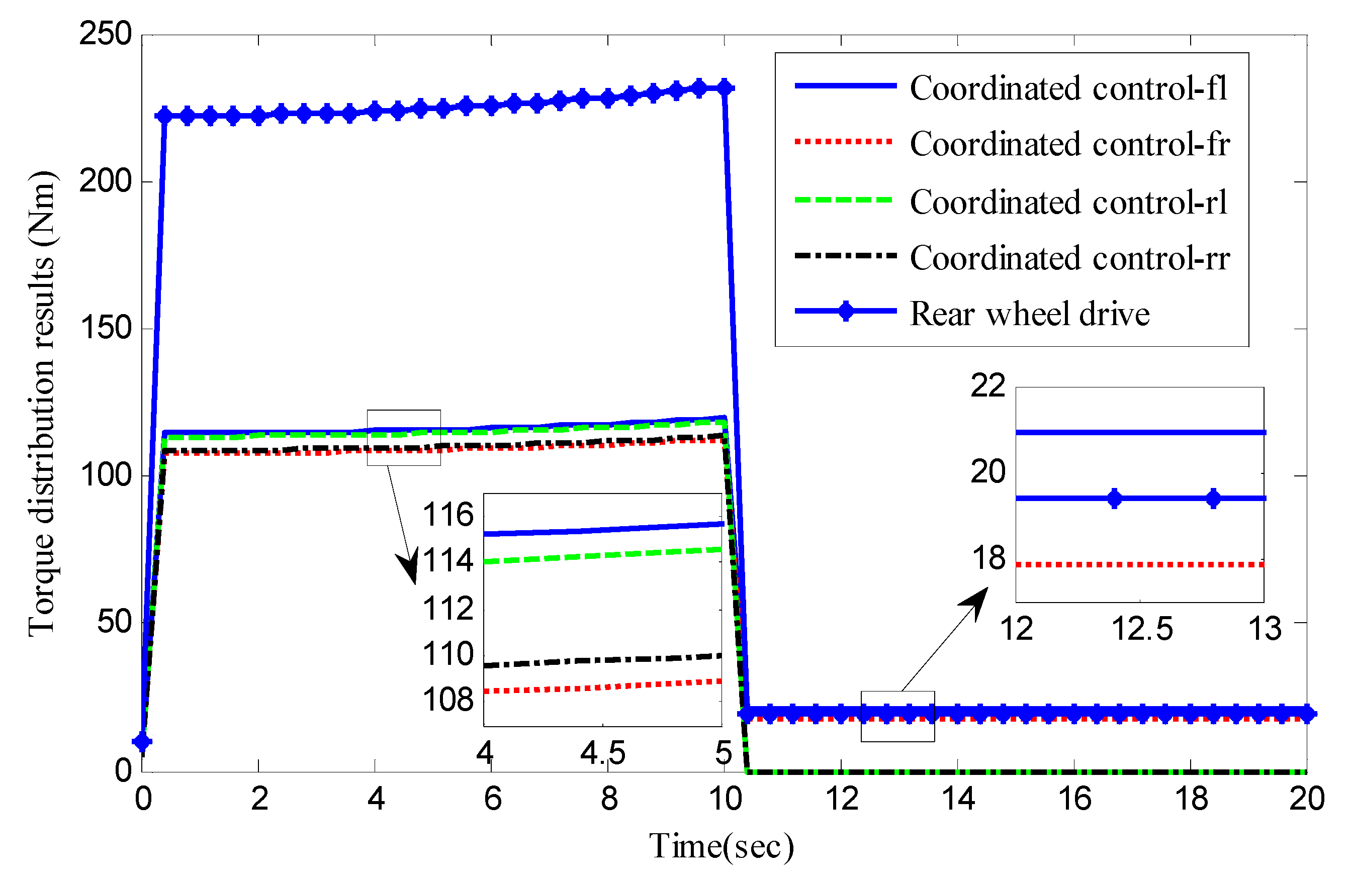
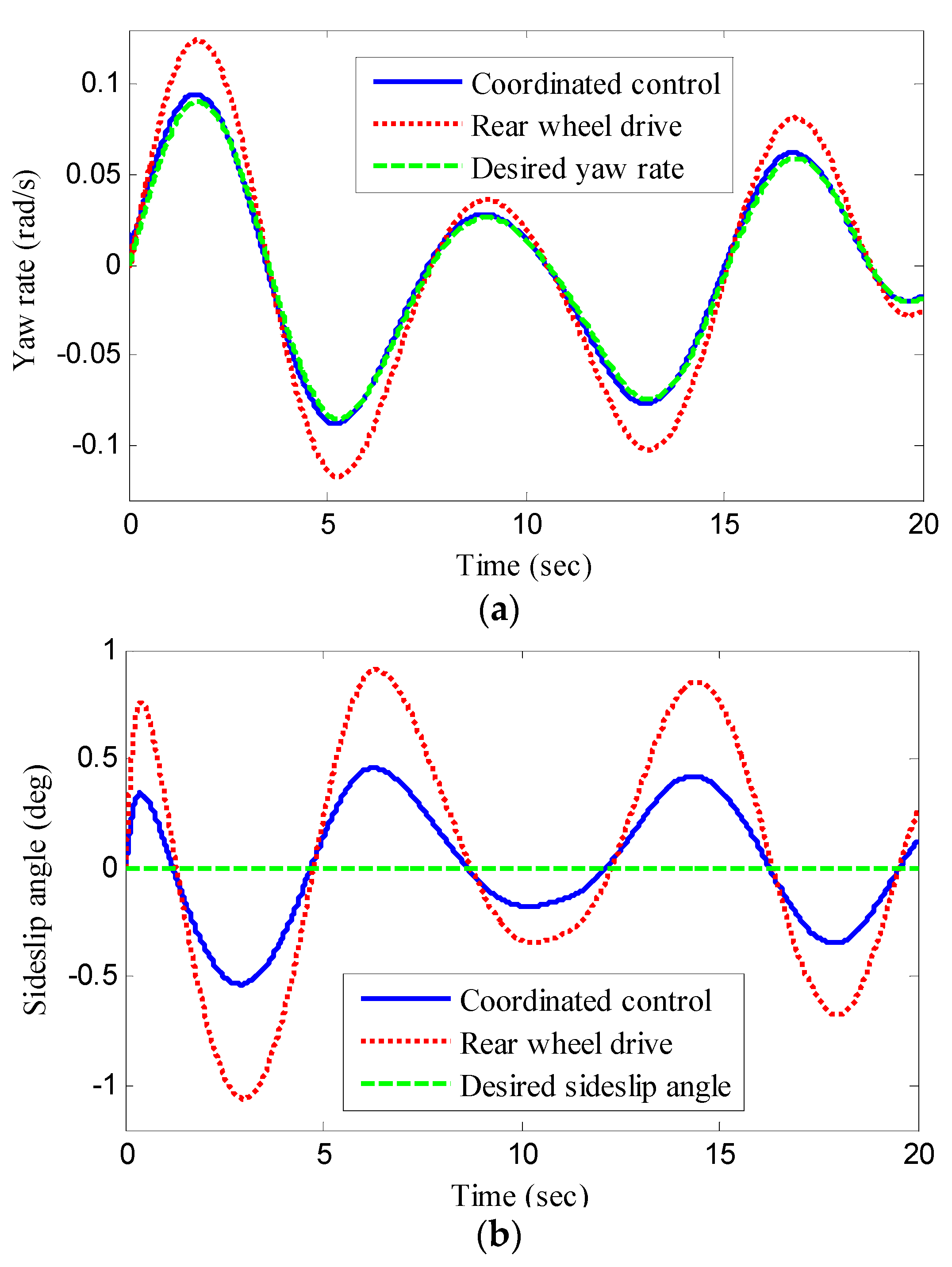
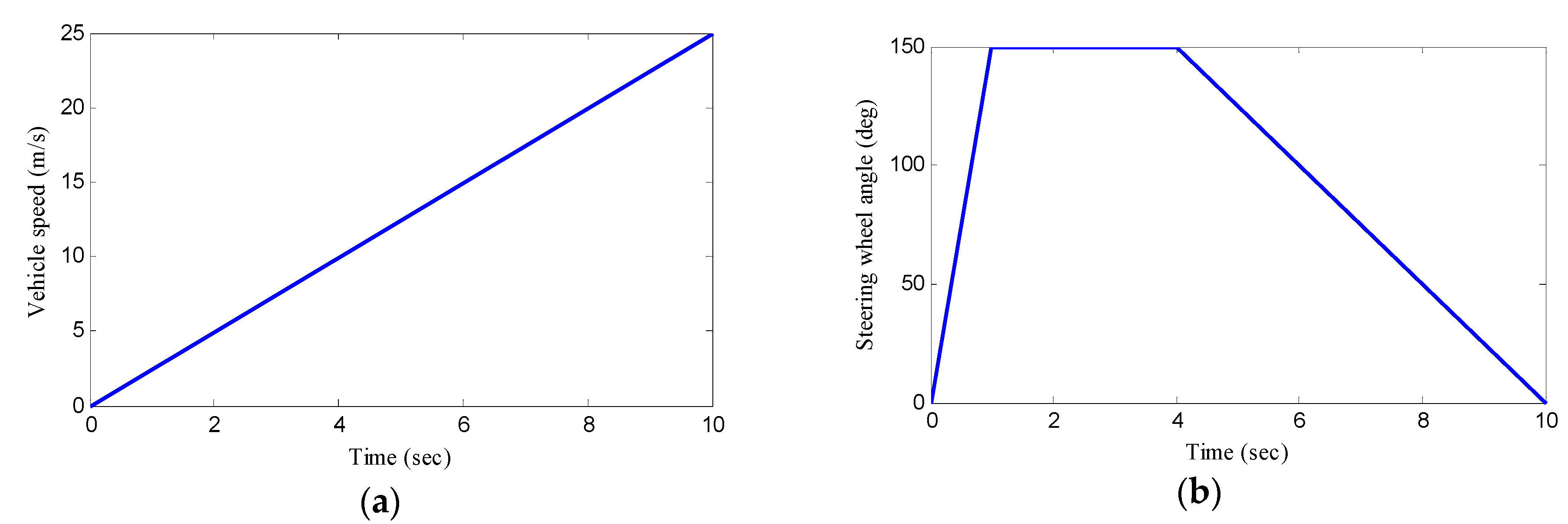
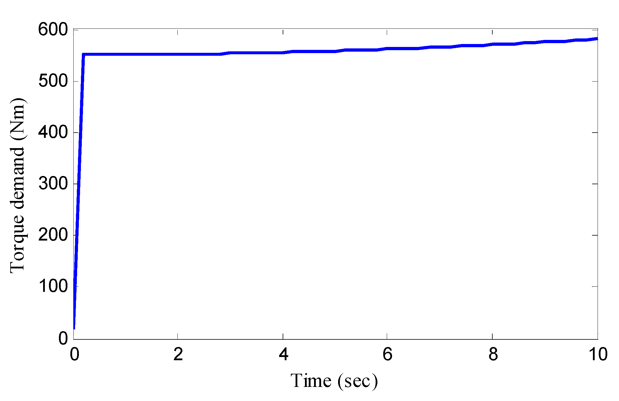
5.2. J-Turn Manoeuver
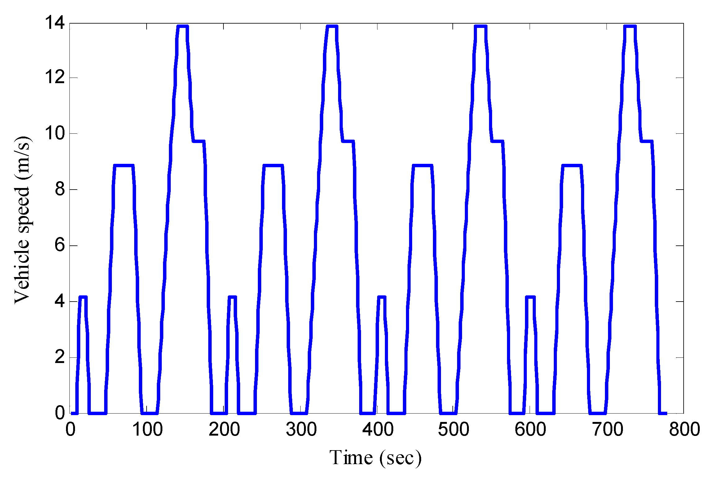
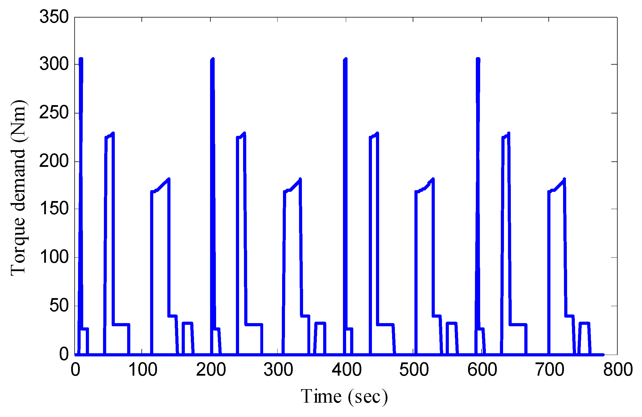
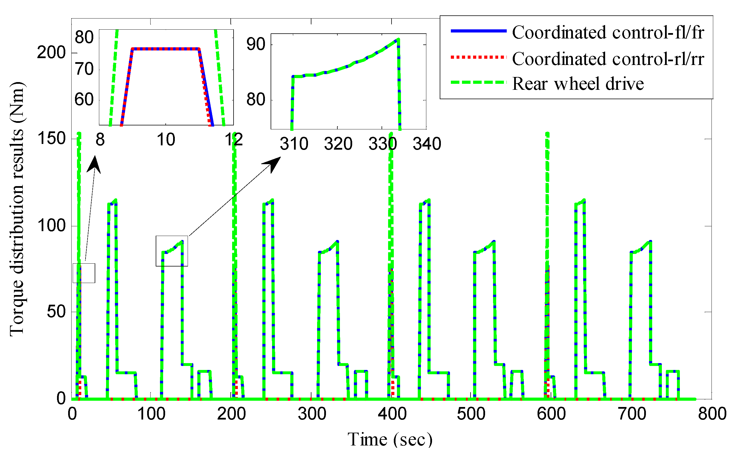
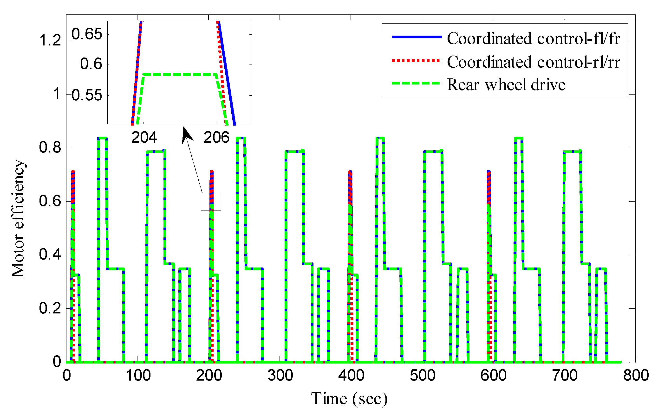
To further verify the proposed control method, in case study 2, the simulation validation of the J-turn manoeuver is carried out to reflect the control effect under the more complex working condition of violent steering. The simulation condition is shown in Figure 13, including the planned vehicle speed and steering wheel angle of the J-turn manoeuver. The road friction coefficient is 0.8 in the simulation. Similarly, according to Equation (21), the demanded torque in case study 2 can be obtained and shown in Figure 14. One can find that the demanded torque in case study 2 is relatively larger than that of case study 1, due to the acceleration manoeuver, which means that the result of the optimal torque allocation is more inclined to four-wheel allocation in coordinated control, so as to reduce the load torque of each single motor, and thereby improving the driving efficiency of the in-wheel motor. The torque distribution results can be seen in Figure 15. It can be found that on the whole, the result of torque distribution tends to be four-wheel average distribution in coordinated control, and there are some differences in the four-wheel drive torque directly to generate an additional yaw moment. In the result of torque allocation of rear-wheel drive, the driving torque of each single motor is greatly increased, which is about twice the driving torque under coordinated control, and will lead to a great reduction in the motor efficiency. The motor efficiency in case study 2 is shown in Figure 16. As shown in Figure 16, the simulation results coincide with our analysis. The motor driving efficiency under coordinated control exceeds 0.7, which is much higher than that under rear-wheel drive. In the same way, the total motor load power is computed and shown in Figure 17. We can find that the energy utilization ratio of the whole vehicle is improved, and the overall load power is greatly reduced under coordinated control. Accordingly, the energy consumption is case study 2 can be achieved, and the energy consumption rates of coordinated control and rear-wheel drive are 247.83 KJ and 134.02 KJ, respectively. The energy consumption is decreased by 45.92%. The vehicle stability control results in case study 2 can be seen in Figure 18. Through comparative analysis, it can be seen that the yaw rate of a vehicle under coordinated control can track the desired yaw rate in real time with good accuracy, while the yaw rate of a vehicle under rear-wheel drive deviates significantly from the desired yaw rate. Moreover, the sideslip angle of coordinated control is also significantly smaller than that under rear-wheel drive. It can be found that the proposed coordinated control method can achieve energy-saving control while ensuring the stability of the vehicle even under severe steering conditions.

5.3. ECE Manoeuver

In order to verify the energy-saving effect of the proposed method under standard operating conditions, the simulation of an economic commission for Europe (ECE) manoeuver is carried out in case study 3. In the simulation of an ECE manoeuver, the steering control of vehicle is not implemented, and only the energy-saving effect under the standard working conditions is verified. The ECE urban cycle manoeuver for simulation is shown in Figure 19, and corresponding demand torque is shown in Figure 20. We can find that the speed under standard conditions is relatively low, and the vehicle demand torque is relatively small. The torque distribution results in case study 3 are shown in Figure 21. One can find that in the first acceleration process, because the demand torque of the vehicle is relatively large, the coordinated control method chooses to reduce the load torque of each single motor by means of the average distribution of the front and rear axles. In the other acceleration and uniform speed processes, because the vehicle needs less torque, the torque distribution results under coordinated control are basically consistent with the rear-wheel drive. The motor efficiency in simulation is shown in Figure 22. It can be found that in the first acceleration process, the motor efficiency under coordinated control is higher than that of rear-wheel drive, and in the other acceleration and uniform speed processes, owning to the same torque distribution results, the motor efficiency under two driving modes is basically the same. In the same way, the total motor load power in case study 3 is computed and shown in Figure 23, and the motor load power of the coordinated control method in the first acceleration process is obviously smaller than that of the rear-wheel drive method. The total energy consumption of the coordinated control method and rear-wheel drive in the ECE urban cycle manoeuver is 2257.54 KJ and 2349.46 KJ, respectively, and the energy consumption is decreased by 4.07%.

6. Conclusions

This paper presents a hierarchical coordinated control method of an in-wheel motor drive electric vehicle based on energy optimization. The driving architecture and control network framework of the electric vehicle is designed using the RPP, and to facilitate and promote the following further research, vehicle modeling in CarSim software is carried out. In order to characterize vehicle dynamics behavior, a bicycle model is established. The efficiency map of the in-wheel motor is drawn and the efficiency characteristics of the motor are analyzed. After that, the energy-saving feasibility analysis of an in-wheel motor drive electric vehicle is carried out. Considering the energy optimization of the whole vehicle, the hierarchical coordinated control method is designed, including an upper layer controller, a middle layer controller, and a lower layer controller. The upper layer controller is used to decide the driving mode of the electric vehicle on the basis of the motor efficiency characteristics. The middle layer controller is used to generate the real-time control quantity of the front-wheel steering angle and an additional yaw moment using sliding mode control. The lower layer controller is used to distribute the tire force according to the driving mode decision from the upper layer controller and the additional yaw moment requirement from the middle layer controller. The simulation verification is implemented in the CarSim Simulink co-simulation platform, and the results show that the presented control method saves 32.14%, 45.92%, and 4.07% of the energy under selected working conditions, and ensures vehicle stability at the same time.

Author Contributions

J.W. is the major author of the paper. He proposed the overall control method and conducted the verification. J.L. participated in the construction of the simulation models and data processing. J.W. wrote this paper.

Funding

This work was supported by the Key Science and Technology Project of Anyang in 2018.

Conflicts of Interest

The authors declare no conflict of interest.

References

  1. Khaligh, A.; Li, Z.H. Battery, Ultracapacitor, Fuel Cell, and Hybrid Energy Storage Systems for Electric, Hybrid Electric, Fuel Cell, and Plug-In Hybrid Electric Vehicles: State of the Art. IEEE Trans. Veh. Technol. 2010, 59, 2806–2814. [Google Scholar] [CrossRef]
  2. Zhang, L.; Zhao, Z.; Chai, J.; Kan, Z. Risk Identification and Analysis for PPP Projects of Electric Vehicle Charging Infrastructure Based on 2-Tuple and the DEMATEL Model. World Electr. Veh. J. 2019, 10, 4. [Google Scholar] [CrossRef]
  3. Chen, T.; Xu, X.; Chen, L.; Jiang, H.B.; Cai, Y.F.; Li, Y. Estimation of longitudinal force, lateral vehicle speed and yaw rate for four-wheel independent driven electric vehicles. Mech. Syst. Signal Process 2018, 101, 377–388. [Google Scholar] [CrossRef]
  4. Wang, R.; Chen, Y.; Feng, D.; Huang, X.; Wang, J. Development and performance characterization of an electric ground vehicle with independently actuated in-wheel motors. J. Power Sources 2011, 196, 3962–3971. [Google Scholar] [CrossRef]
  5. Iora, P.; Tribioli, L. Effect of ambient temperature on electric vehicles’ energy consumption and range: model definition and sensitivity analysis based on nissan leaf data. World Electr. Veh. J. 2019, 10, 2. [Google Scholar] [CrossRef]
  6. Zhai, L.; Hou, R.F.; Sun, T.M.; Kavuma, S. Continuous steering stability control based on an energy-saving torque distribution algorithm for a four in-wheel-motor independent-drive electric vehicle. Energies 2018, 11, 350. [Google Scholar] [CrossRef]
  7. Lin, C.; Xu, Z.F. Wheel torque distribution of four-wheel-drive electric vehicles based on multi-objective optimization. Energies 2015, 8, 3815–3831. [Google Scholar] [CrossRef]
  8. Fiori, C.; Ahn, K.; Rakha, H.A. Power-based electric vehicle energy consumption model: Model development and validation. Appl. Energy 2016, 168, 257–268. [Google Scholar] [CrossRef]
  9. Laurikko, J.; Granström, R.; Haakana, A. Realistic estimates of EV range based on extensive laboratory and field tests in Nordic climate conditions. World Electr. Veh. J. 2013, 6, 192–203. [Google Scholar] [CrossRef]
  10. Wang, Y.; Fujimoto, H.; Hara, S. Torque distribution-based range extension control system for longitudinal motion of electric vehicles by LTI modeling with generalized frequency variable. IEEE/ASME Trans. Mechatron. 2016, 21, 443–452. [Google Scholar] [CrossRef]
  11. Chen, Y.; Li, X.; Wiet, C.; Wang, J. Energy management and driving strategy for in-wheel motor electric ground vehicles with terrain profile preview. IEEE. Trans. Ind. Inf. 2014, 10, 1938–1947. [Google Scholar] [CrossRef]
  12. Wang, D.; Yang, F.; Gan, L.; Li, Y. Fuzzy prediction of power lithium ion battery state of function based on the fuzzy c-means clustering algorithm. World Electr. Veh. J. 2019, 10, 1. [Google Scholar] [CrossRef]
  13. Gogoana, R.; Pinson, M.B.; Bazant, M.Z.; Sarma, S.E. Internal resistance matching for parallel-connected lithium-ion cells and impacts on battery pack cycle life. J. Power Sources 2014, 252, 8–13. [Google Scholar] [CrossRef]
  14. Campestrini, C.; Keil, P.; Schuster, S.F.; Jossen, A. Ageing of lithium-ion battery modules with dissipative balancing compared with single-cell ageing. J. Energy Storage 2016, 6, 142–152. [Google Scholar] [CrossRef]
  15. Wang, R.R.; Hu, C.; Wang, Z.J.; Yan, F.J.; Chen, N. Integrated optimal dynamics control of 4WD4WS electric ground vehicle with tire-road frictional coefficient estimation. Mech. Syst. Signal Process 2015, 60–61, 727–741. [Google Scholar] [CrossRef]
  16. Chen, T.; Xu, X.; Li, Y.; Wang, W.J.; Chen, L. Speed-dependent coordinated control of differential and assisted steering for in-wheel motor driven electric vehicles. Proc IMechE Part D: J Auto. Eng. 2018, 232, 1206–1220. [Google Scholar] [CrossRef]
  17. Chen, T.; Chen, L.; Xu, X.; Cai, Y.; Jiang, H.; Sun, X. Estimation of longitudinal force and sideslip angle for intelligent four-wheel independent drive electric vehicles by observer iteration and information fusion. Sensors 2018, 18, 1268. [Google Scholar] [CrossRef] [PubMed]
  18. Jin, X.J.; Yin, G.D.; Chen, N. Gain-scheduled robust control for lateral stability of four-wheel-independent-drive electric vehicles via linear parameter-varying technique. Mechatronics 2015, 30, 286–296. [Google Scholar] [CrossRef]
  19. Wang, R.R.; Zhang, H.; Wang, J.M.; Yan, F.J.; Chen, N. Robust lateral motion control of four-wheel independently actuated electric vehicles with tire force saturation consideration. J. Frankl. Inst. 2015, 352, 645–668. [Google Scholar] [CrossRef]
  20. Nam, K.; Fujimoto, H.; Hori, Y. Lateral stability control of in-wheel-motor-driven electric vehicles based on sideslip angle estimation using lateral tire force sensors. IEEE Trans. Veh. Technol. 2012, 61, 1972–1985. [Google Scholar]
  21. Li, B.Y.; Du, H.P.; Li, W.H.; Zhang, Y.J. Side-slip angle estimation based lateral dynamics control for omni-directional vehicles with optimal steering angle and traction/brake torque distribution. Mechatronics 2015, 30, 348–362. [Google Scholar] [CrossRef]
  22. Chen, Y.; Wang, J. Fast and global optimal energy-efficient control allocation with applications to over-actuated electric ground vehicles. IEEE Trans. Control Syst. Technol. 2012, 20, 1202–1211. [Google Scholar] [CrossRef]
  23. Chen, Y.; Wang, J. Adaptive energy-efficient control allocation for planar motion control of over-actuated electric ground vehicles. IEEE Trans. Control Syst. Technol. 2014, 22, 1362–1373. [Google Scholar]
  24. Dizqah, A.; Lenzo, B.; Sorniotti, A.; Gruber, P.; Fallah, S.; Smet, J. A fast and parametric torque distribution strategy for four-wheel-drive energy-efficient electric vehicles. IEEE Trans. Ind. Electron. 2016, 63, 4367–4376. [Google Scholar] [CrossRef]
Figure 1. Driving architecture and control network framework of the electric vehicle.
Wevj 10 00015 g001
Figure 2. Vehicle modeling in CarSim.
Wevj 10 00015 g002
Figure 3. Vehicle dynamic model.
Wevj 10 00015 g003
Figure 4. Efficiency map of an in-wheel motor.
Wevj 10 00015 g004
Figure 5. Overall control strategy.
Wevj 10 00015 g005
Figure 6. Optimization results of rear-axle torque distribution coefficient.
Wevj 10 00015 g006
Figure 7. Simulation condition in case study 1. (a) Planned vehicle speed; (b) Planned double lane change trajectory.
Wevj 10 00015 g007
Figure 8. Torque demand in case study 1.
Wevj 10 00015 g008
Figure 9. Torque distribution results in case study 1.
Wevj 10 00015 g009
Figure 10. Motor efficiency in case study 1.
Wevj 10 00015 g010
Figure 11. Total motor load power in case study 1.
Wevj 10 00015 g011
Figure 12. Results of vehicle stability control in case study 1. (a) Yaw rate; (b) Sideslip angle.
Wevj 10 00015 g012
Figure 13. Simulation condition in case study 2. (a) Planned vehicle speed; (b) Steering wheel angle.
Wevj 10 00015 g013
Figure 14. Torque demand in case study 2.
Wevj 10 00015 g014
Figure 15. Torque distribution results in case study 2.
Wevj 10 00015 g015
Figure 16. Motor efficiency in case study 2.
Wevj 10 00015 g016
Figure 17. Total motor load power in case study 2.
Wevj 10 00015 g017
Figure 18. Results of vehicle stability control in case study 2. (a) Yaw rate; (b) Sideslip angle.
Wevj 10 00015 g018
Figure 19. Economic commission for Europe (ECE) urban cycle manoeuvr in case study 3.
Wevj 10 00015 g019
Figure 20. Torque demand in case study 3.
Wevj 10 00015 g020
Figure 21. Torque distribution results in case study 3.
Wevj 10 00015 g021
Figure 22. Motor efficiency in case study 3.
Wevj 10 00015 g022
Figure 23. Total motor load power in case study 3.
Wevj 10 00015 g023
Table 1. Vehicle parameters in CarSim simulation model.
SymbolParametersValue and Units
mVehicle mass850 kg
rEffective radius of wheel0.25 m
lfDistances from vehicle gravity center to the front axle0.815 m
lrDistances from vehicle gravity center to the rear axle0.985 m
bf, brHalf treads of the front(rear) wheels0.78 m
CfEquivalent cornering stiffness of front wheel65,000 N/rad
CrEquivalent cornering stiffness of rear wheel45,000 N/rad
IzMoment of inertia1000 kg·m2
REquivalent resistance of winding0.675 Ω
KaInverse electromotive force coefficient0.065 Nm/A
KtMotor torque constant11.425 Nm/A
JSum of inertia moment of wheel and motor7.165 kg·m2
bDamping coefficient0.645 Nm·sec/rad
LEquivalent inductance of winding0.125H

