Article

Explainable and Analyst-Driven Random Forest for Intrusion Detection

1
National School of Computer Science and Systems Analysis (ENSIAS), Mohammed V University in Rabat, Rabat 10100, Morocco
2
Department of Engineering Technology (INDI), Vrije Universiteit Brussel, Pleinlaan 2, 1050 Brussels, Belgium
*
Author to whom correspondence should be addressed.
Future Internet 2026, 18(9), 490; https://doi.org/10.3390/fi18090490 (registering DOI)
Submission received: 2 August 2026 / Revised: 2 September 2026 / Accepted: 15 September 2026 / Published: 18 September 2026
(This article belongs to the Section Cybersecurity)

Abstract

Random Forest and other tree-ensemble classifiers achieve high accuracy in network intrusion detection; however, their aggregate decision logic prevents analysts from auditing or deploying individual predictions as operational rules. Post hoc explanation methods introduce latencies incompatible with security operation center (SOC) requirements and produce conditions unsuitable for firewall configuration. Among the systems reviewed in this study, none unifies intrinsic explanation, rule deployment, ATT&CK attribution, cross-dataset validation, and adaptive feedback in one pipeline. This work presents a depth-limited Random Forest with deterministic, per-instance explanations at a fraction of gradient-based attribution latency. Complementary mechanisms generate analyst-deployable rule specifications, technique-level adversary attribution, and a feedback protocol that models label noise, missed reviews, and bounded correction budget. Evaluated on a large, multi-category network-traffic benchmark, the system attains high detection accuracy (macro recall 0.86 , driven substantially by the majority normal-traffic class at 68 % of flows) while sustaining throughput beyond SOC requirements; a stealthy reconnaissance-and-exploitation category remains markedly harder to detect under this class imbalance. Cross-dataset evaluation on a more recent benchmark attains strong performance after limited target-domain retraining. The adaptive feedback protocol yields a statistically significant false-positive reduction over repeated simulated reviews, requiring only modest weekly analyst effort. Together, these capabilities enable auditable and SOC-integrable detection pipelines.

1. Introduction

The increasing number of attacks on computer networks has put immense pressure on SOC operations. Therefore, SOCs require an intrusion detection system (IDS) that operates effectively in SOC-compatible conditions, while providing high accuracy and transparency [1]. Signature-based IDS detect known attacks in 70–95% of cases; however, they fail to recognize new threats and generate false-positive volumes that exceed the capacity of SOC analysts [2,3]. Machine learning-based intrusion detection systems (ML-IDS) offer significant improvements in detecting attacks, with accuracies for Random Forest (RF), XGBoost, and deep learning algorithms reported in the range of 90–98% based on benchmarking data [4,5]. A comprehensive cross-dataset study showed that although machine learning models perform almost perfectly on a given dataset, their accuracy decreases significantly when applied to a new unseen network [6]. However, ML models face a practical limitation: their decision logic is opaque, making them difficult to understand, audit, and challenge [6]. Self-supervised learning approaches have demonstrated the ability to reduce dependence on attack-labeled data while maintaining competitive detection performance across diverse network environments [7]. Moreover, regulatory requirements, such as the General Data Protection Regulation (GDPR), stipulate the necessity of providing rationales for algorithmic decisions [8], reinforcing transparency as a primary design requirement.
ML-based IDS approaches in the current literature share three operational limitations, motivating the Random Forest-specific focus of this work. First, Random Forest and related ensembles of decision tree learners such as XGBoost expose only the aggregate feature importance at the ensemble level without providing any individual decision thresholds that can be used to configure firewalls [5,6,9]. Second, deep neural networks have substantial weaknesses in terms of stealthy and low-frequency attacks. For instance, in the full-class test suite of CSE-CIC-IDS2018, deep neural networks and convolutional neural networks yielded F1-scores of 0% and 4.73% for the Infiltration categories, respectively, [10], indicating that macro-accuracy does not imply model robustness. Third, most reviewed ML-based IDS studies were evaluated on a single benchmark dataset, providing insufficient evidence of robustness across heterogeneous SOC environments with different network monitoring infrastructures and feature extractors [11,12].
Several approaches based on explainable artificial intelligence (XAI) techniques have been developed to address this transparency deficit. The use of post hoc methods, such as Local Interpretable Model-agnostic Explanations (LIME) [13] and SHapley Additive explanations (SHAP) [14], is a common practice in the considered studies and is applied as separate downstream steps after classification. Although these methods improve analyst understanding in controlled settings, they introduce a per-instance latency of 15–300 ms, which is generally incompatible with the sustained SOC throughput requirements [15]. Beyond latency, attributions computed by post hoc approaches provide a quantified measure of the marginal importance of features; however, they do not specify the exact threshold conditions under which the classifier changes its output. Thus, SOC analysts cannot retrieve the decision condition from an alert record, which limits their ability to audit, challenge, or document individual classification decisions [16]. In addition, LIME suffers from output variance from repeated queries of identical inputs [17,18]. Both LIME and SHAP lack the criteria by which a classifier decides to change its decisions, implying that the decision-making process cannot be inferred from an attribution trace alone [16,19]. The combination of these shortcomings renders any such process incapable of providing the consistent audit trail required for SOC-reportable incidents [16].
Six limitations (G1–G6) were identified in the reviewed literature: (G1) post hoc latency and stochastic inconsistency; (G2) an absence of IF-THEN rules with raw-unit thresholds usable for firewall configuration; (G3) a lack of SOC-compatible MITRE ATT&CK attribution within the classification forward pass; (G4) insufficient cross-dataset validation across incompatible feature extractors; (G5) an absence of statistically validated adaptive feedback that models analyst label noise, missed review rounds, and bounded weekly correction budgets; and (G6) no unified pipeline simultaneously addressing detection, intrinsic explanation, rule deployment, ATT&CK mapping, cross-dataset adaptation, and validated adaptive feedback under sustained SOC throughput conditions. These six limitations were systematically surveyed and mapped against the 12 representative studies listed in the comparison table in Section 2 [16,19].
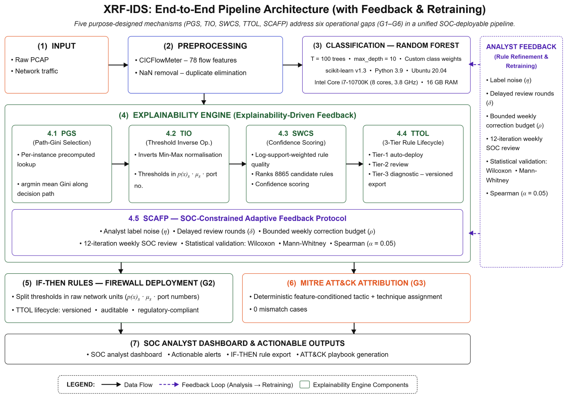
This study proposes an eXplainable Random Forest Intrusion Detection System (XRF-IDS) that jointly integrates intrinsic explainability, raw-unit IF-THEN rule deployment, SOC-compatible MITRE ATT&CK mapping, cross-dataset adaptation, and statistically validated adaptive feedback within a single SOC-oriented detection pipeline. XRF-IDS employs depth-limited RF ( T = 100 trees, max_depth = 10 ) and introduces five purpose-designed mechanisms: Path-Gini Selection (PGS), Threshold Inverse Operationalization (TIO), Support-Weighted Confidence Score (SWCS), Three-tier Operational Lifecycle (TTOL), and SOC-Constrained Adaptive Feedback Protocol (SCAFP), as illustrated in Figure 1 and formalized in Section 3.
The novelty of this study is established relative to the two closest prior directions identified in Section 2. Relative to post hoc explanation frameworks for intrusion detection [13,14,16,17], which compute feature attributions after classification at a measured cost of 15–300 ms per flow [15] and do not guarantee agreement with the underlying ensemble decision, the proposed path-selection criterion is computed within the standard forest prediction call, achieves empirically measured fidelity against the ensemble majority vote, and has not been proposed in this form in the surveyed literature. Relative to prior rule-extraction systems that report split thresholds in the normalized feature space and require manual back-transformation before deployment, the threshold reconstruction, confidence-support ranking, and tiered deployment lifecycle introduced here operationalize selected decision paths directly into raw-unit rule specifications, avoiding the manual back-transformation step required by prior methods. The contributions of this work span algorithmic design, specifically the per-instance PGS criterion, three-parameter SCAFP protocol, and system-level integration, jointly enabling SOC-compatible deployment under operational constraints. The main contributions of this study are as follows:
  • Path-Gini Selection with operationalized rule deployment (PGS + TIO/SWCS/TTOL). The PGS selects the representative decision path per classified flow as t * = arg min t G t ( x ) , where G t ( x ) is the mean Gini impurity along tree t root-to-leaf paths. Unlike population-level rule extraction methods [20,21], the PGS operates per instance without incurring additional inference costs. Three complementary mechanisms operationalize the selected path: TIO reconstructs split thresholds in raw network units; SWCS ranks candidate rules using a log-support-weighted confidence score; and TTOL organizes rules into three deployment tiers with automated versioning. The full formalization is presented in Section 3.5 and Section 3.6.
  • SOC-compatible ATT&CK attribution and cross-dataset adaptation. XRF-IDS assigns MITRE ATT&CK tactics and technique identifiers simultaneously with classification through a deterministic feature-conditioned function at a sub-microsecond overhead without an external knowledge base [22,23,24]. The cross-dataset evaluation of NF-ToN-IoT-v3 [11,25] (2025) and NF-UNSW-NB15-v2 (2015) across five labeling budgets identified the optimal adaptation of the operating points. The details are provided in Section 4.5 and Section 4.6.
  • SCAFP: Statistically validated adaptive feedback under realistic SOC constraints. SCAFP jointly parameterizes analyst label noise ( η ), missed review rounds ( δ ), and bounded weekly correction budget ( ρ ) constraints, which were absent in previous protocols [26,27]. Improvement was validated through three non-parametric tests, and ablation analysis was used to isolate the contribution of each operationally critical parameter. Details are provided in Section 3.8 and Section 4.7.

2. Related Work

This section surveys representative IDS research across four streams: ML-based detection, XAI applied to IDS, SOC-oriented and deployable systems, and adaptive or online learning mechanisms.

2.1. Machine Learning-Based Intrusion Detection

Ensemble classifiers, particularly RF, have achieved detection accuracies of 90–99% on established benchmarks, including CICIDS2017, CSE-CIC-IDS2018, and UNSW- NB15 [4,5,6,28,29]. Le et al. [4] and Patil et al. [5] demonstrated that RF delivers consistent multiclass accuracy on Internet of Things (IoT) and enterprise network datasets.
Patidar et al. [28] confirmed the effectiveness of RF in the CSE-CIC-IDS2018. Bilal et al. [25] surveyed secure and explainable federated learning for IoT intrusion detection, and Eren et al. [30] proposed a machine learning-based IoT intrusion detection system that combines RF with Explainable Boosting-Like Regression (EBLR)-based feature generation and smart preprocessing, achieving an F1-score of 0.994 and AUC of 0.99 on ToN-IoT datasets, rivaling deep learning approaches while maintaining interpretability. Hajj et al. [29] reported 99.99% accuracy for CSE-CIC-IDS2018 using XGBoost with PCA-based feature reduction, although this result excluded the challenging Infiltration category. Deep learning architectures achieve high overall accuracy in volumetric attacks but demonstrate significant weaknesses in stealthy categories. Cheng et al. [10] reported DNN and CNN Infiltration F1 scores of 0% and 4.73%, respectively, for a full-class CSE-CIC-IDS2018. Chen et al. [31] combined deep learning and SHAP feature selection on CICIDS2017 and IoT datasets without delivering actionable rule artifacts or cross-dataset validation of these results. Their common weakness lies in their emphasis on accuracy, which does not translate into deployability. Interpretability is limited to feature importance, validation is performed against a single dataset, and there is no approach to move from model training to SOC deployment.

2.2. Explainable AI for Intrusion Detection

2.2.1. Post Hoc Explanation Methods

Post hoc XAI is the dominant paradigm in this area. LIME [13] and SHAP [14] were applied after classification to generate local feature attributes. Gaspar et al. [32] demonstrated through user surveys that LIME and SHAP improve analysts’ interpretability in an MLP-based IoT IDS. Arreche et al. [17] systematically evaluated both methods across seven models and three datasets using quality metrics including stability, efficiency, and robustness. Hermosilla et al. [33] evaluated SHAP and LIME for forensic legal defensibility using XGBoost and TabNet models, and Nugraha et al. [34] combined XGBoost with ANOVA feature selection and post hoc explanations to approach near-real-time throughput.
Even with these improvements, post hoc techniques suffer from the same structural drawbacks outlined in Section 1: instance-level delay incompatible with SOC throughput, randomness of output values in LIME [17,18], and no specified thresholds for attribution values [16]. XRF-IDS addresses these limitations using PGS and TIO.

2.2.2. Multi-Model Benchmarks

Arreche et al. [17] evaluated SHAP and LIME on seven black-box models, achieving approximately 99% accuracy but leaving models as opaque predictors with no deployable rule output. Mohale and Obagbuwa [19] compared LIME, SHAP, and ELI5 on five classifiers, reported an accuracy of approximately 87%, and explicitly identified SOC-compatible deployment as an unresolved challenge. Systematic surveys by Neupane et al. [16] and Mohale and Obagbuwa [19] confirmed that post hoc latency and the absence of standardized analyst-facing explanation formats are the primary barriers to IDS deployment in SOC environments. Kalasampath et al. [35] provided a comprehensive literature review of XAI applications in IDS, identifying deployable rule generation and cross-validation as the two most frequently unaddressed gaps in the surveyed systems.

2.2.3. Intrinsic Interpretability Approaches

Unlike post hoc methods that approximate decision rules and present attribute values within normalized features, intrinsic methodologies natively implement transparency in the model architecture while presenting natural decision rules, yet create semantic differences between the normalized threshold values reported and network units used by SOC analysts, as highlighted in [16]. As noted in Section 1 (G2), single decision trees generate native IF-THEN rules but suffer from high variance in high-dimensional network traffic [20,29]. Decision tree rule extraction from RFs using RDTIDS [20] and inTrees [21] filters and ranks ensemble decision paths, but presents normalized feature values that cannot be verified against the network monitoring dashboard by SOC analysts without performing back-transformation [16]. This semantic gap reduces the usability of the generated rules, even when they are syntactically correct. XRF-IDS solves this problem using PGS and TIO, which work on an instance basis and in terms of raw network units, respectively, as explained in Section 3.5 and Section 3.5.3.
Beyond RDTIDS and inTrees, recent rule-extraction methods target the same interpretability-fidelity trade-off. Obregon and Jung [36] propose RuleCOSI+, which extracts compact rule sets from classification tree ensembles by combining and simplifying candidate rule paths, improving on population-level frequency ranking, while methods such as RDTIDS and inTrees operate on normalized feature representations without addressing SOC-unit deployability. Adewole et al. [37] integrated rule induction directly into an ensemble-based IoT IDS pipeline, validating extracted IF-THEN rules against held-out test data and reporting per-rule precision, although their rules remain in normalized feature space and are not mapped to MITRE ATT&CK or exported to signature-engine formats.
Beyond feature-attribution and rule-extraction outputs, a parallel body of work examines whether explanations translate into operator action. Rastogi et al. [38] conducted a mixed-methods study (a 248-respondent survey and 24 analyst interviews) evaluating which explanation formats SOC analysts perceive as actionable and trustworthy under time pressure, finding that a persistent gap separates academic XAI prototypes from deployment-ready, operationally integrated systems. This finding directly motivates the SOC-deployable design constraints (raw-unit rules, MITRE mapping, tiered auto-deployment) that distinguish XRF-IDS from attribution-only explanation methods.

2.3. SOC-Oriented and Deployable IDS Systems

2.3.1. MITRE ATT&CK Integration

The MITRE ATT&CK framework presents a standardized taxonomy of 193 adversary techniques spanning 14 tactics that are prevalent in SOC threat intelligence and playbook creation [39,40]. Maniyat and Reddy [24] annotated 973 Snort rules based on ATT&CK tactics and techniques using machine learning algorithms and large language models, although their system annotated pre-existing signature rules rather than learned classifier outputs and was not integrated into a real-time detection pipeline. Conversely, knowledge graph mapping assigns ATT&CK tactics and techniques at 100–200 ms per operation, exceeding live SOC alert requirements [22,23]. In addition, auto-MITRE text-based mapping attains an accuracy of 82%–88% but requires unstructured textual input unavailable from raw network flow data [23]. In their XAI-powered IoT IDS, Hulayyil et al. [41] augmented analyst confidence using explanation dashboards but lacked ATT&CK mapping. Among the systems examined in this review, none have demonstrated deterministic technique attribution in conjunction with flow-based classification in submilliseconds, unlike the approaches in [22,23,24]. XRF-IDS addresses this limitation by performing ATT&CK attribution using a feature-based function during the classification process (Section 3.7 and Section 4.5).

2.3.2. Cross-Dataset Generalization Gap

The domain gap between incompatible feature extractors (G4, Section 1) is a well-documented deployment barrier [11,12]. Sarhan et al. [11] empirically quantified this gap. Cross-dataset validation using genuinely incompatible extractors has seldom been reported in the literature. XRF-IDS addresses this gap in Section 4.6.

2.3.3. Operational Deployment Pipelines

As summarized in Table 1, none of the twelve representative systems surveyed in this review provide a complete pipeline from detection to SOC deployment: no reviewed work reports threshold-specific IF-THEN rules in raw network units, unlike RDTIDS and inTrees [20,21], which the present work adopts as re-implemented baselines, automated rule versioning and retirement linked to retraining cycles, or validated throughput across multiple SOC deployment scenarios [16].

2.4. Adaptive and Online Intrusion Detection

Concept drift degrades the performance of static IDS classifiers [15,26]. Although Seth et al. [26] and Martindale et al. [27] focused on drift correction for streaming IDS problems, they failed to model the real-world constraints associated with feedback from SOC analysts, including realistic label noise rates, missed feedback rounds, and bounded weekly review budgets. Online adaptive methods such as Hoeffding Trees, Adaptive Random Forest, and DRIFTNET-EnVACK [15] update models per-flow without human intervention and batch retraining, thereby achieving rapid automated adaptation to concept drift. However, none of the online methods surveyed in this review generate analyst-deployable IF-THEN rules in raw network units, model analyst label noise or correction budget constraints, or provide statistically validated feedback improvement under realistic SOC operational conditions [3,16]. SCAFP is specifically designed for SOC operational rhythms in which weekly analyst review cycles, audit trail requirements, and explainable rule deployment take precedence over per-flow autonomous adaptation. This is a design choice, not a limitation. On the other hand, Bilal et al. [25] and Hulayyil et al. [41] highlight adaptability as a design constraint without providing evidence through hypothesis testing. A common issue in both the studies was that they lacked statistical validation under realistic constraints. In contrast, SCAFP overcomes this issue by explicitly modeling the operational constraints in the feedback process, as discussed in Section 3.8.

2.5. Synthesis and Positioning of XRF-IDS

As established in Section 1 (G1–G6), Table 1 shows that none of the 12 surveyed works addressed more than one of these gaps simultaneously. Among the twelve representative works surveyed, none address more than one of these six gaps simultaneously, let alone under the sustained SOC throughput conditions a shortfall XRF-IDS is designed to close, as detailed in Section 3.
For XRF-IDS, the six gaps are addressed as follows: G1 via PGS (Section 3.5); G2 via TIO raw-unit rule generation (Section 3.6), with SOC deployment as illustrative templates (Section 3.6); G3 via deterministic MITRE ATT&CK mapping, an implementation-correctness check rather than expert-validated accuracy (Section 3.7); G4 via cross-dataset adaptation (Section 3.4); G5 marked partial, as SCAFP’s FPR reduction trend is supported by a Spearman trend correlation surviving multiple-comparison correction but not by all originally reported tests (Section 3.8); and G6 via the unified five-mechanism pipeline (Section 3). As explained in Section 2.5, the bagging architecture of Random Forest uniquely enables the PGS path-selection mechanism described below. In contrast, in gradient boosting ensembles (e.g., XGBoost, LightGBM), each tree encodes an incremental correction to the residual error of the previous ensemble state; therefore, no single boosting tree is a complete, independently valid classifier, and PGS’s per-instance path-selection semantics do not transfer to boosting architectures without a fundamentally different formulation. Deep neural networks lack any comparable discrete decision-path structure, precluding TIO threshold reconstruction and requiring post hoc attribution methods with the latency and non-determinism limitations discussed above (Section 2). Empirically, the baseline results confirm RF retains competitive accuracy (97.57%) and the highest macro precision (0.9704) against XGBoost and LightGBM baselines evaluated under identical conditions, while a single decision tree is interpretable in the same sense but without ensemble averaging trails substantially (80.75% accuracy). This motivates RF as the architecture that jointly satisfies accuracy and the structural requirements of intrinsic, per-instance, deterministic explanation.

3. Methodology

The XRF-IDS pipeline integrates five purpose-designed mechanisms, each addressing a specific gap identified in Section 2: (1) PGS (Section 3.5), (2) TIO (Section 3.6), (3) SWCS (Section 3.6), (4) TTOL (Section 3.6), and (5) SCAFP (Section 3.8). All experiments were conducted on an Ubuntu 20.04, with an Intel Core i7-10700K (8 cores, 3.8 GHz), 16 GB RAM, and a 512 GB NVMe SSD, using Python 3.9 and Scikit-learn v1.3.
Figure 1 presents the end-to-end architecture of XRF-IDS, illustrating how the five mechanisms operate sequentially within a unified SOC-deployable pipeline.

3.1. Dataset and Preprocessing

Dataset

The main dataset used was CSE-CIC-IDS2018 [12], a publicly available benchmark of network intrusion data, in which 78 bidirectional features were extracted from raw PCAP captures using CICFlowMeter. The seven daily CSV files (14, 23, 26, 27, 28 February and 1, 2 March 2018) were concatenated. After concatenating, cleaning (removal of NaN/Inf and duplicates), and unifying labels, the corpus contained six raw label groups, of which the ’WebAttack’ group contained fewer than 500 samples and was dropped because of insufficient counts for reliable estimation. After the exclusion and unification of the remaining labels, the curated dataset comprised 2,162,527 instances across five classes: Normal, Botnet, BruteForce, DoS, and Infiltration. Table 2 details the label unification performed during curation. Each merged class includes multiple raw attack subtypes present in the CSE-CIC-IDS2018 dataset. The attacks were classified based on their observable behavior in the network, rather than the attack tool used. The BruteForce category includes credential-stuffing attacks using three protocols: FTP (FTP-Patator and FTP-BruteForce), SSH (SSH-Patator and SSH-Bruteforce), and HTTP form-authentication attacks (BruteForce web). The sub-category BruteForce-XSS was also included in this category because it is a form of a BruteForce attack rather than client-side injection. Distinct XSS and SQL Injection labels, both pure injection attacks, were assigned to WebAttack and were subsequently excluded. The DoS category comprises seven subtypes sharing the same network signature, namely, connection exhaustion or volumetric flooding: Hulk, GoldenEye, Slowloris, SlowHTTPTest (slow-rate HTTP attacks), and LOIC-HTTP, LOIC-UDP, and HOIC (volumetric DDoS). The Botnet corresponds to the ARES Botnet command-and-control (C&C) communication. Infiltration involves a multiple-step attack: Nmap port scanning (Phase 1 reconnaissance), Metasploit exploitation of Windows Vista (Phase 2), and backdoor communication (Phase 3). Port scanning is thus present in the dataset as Phase 1 of the Infiltration category, although the three phases have just one category label that leads to a high level of heterogeneity within the features of this class, which results in a lower recall than the others. WebAttack (XSS and SQL Injection) was removed during the curation process because of a lack of sufficiency (<500 flows).
Table 3 reports per-class counts, proportions, imbalanced ratios, and assigned weights to the two partitions.
The four operations are applied in the following order: removal of rows containing NaN, Inf, or −Inf values, removal of duplicate flow records, exclusion of the WebAttack class, and min–max normalization of all 78 features to [ 0 , 1 ] , using parameters fitted exclusively on the training partition to prevent data leakage.
A stratified 70/30 split yielded 1,513,768 training flows and 648,759 test flows. The number of trees ( T = 100 ) follows standard Random Forest practice; the depth constraint ( max _ depth = 10 ) was selected primarily for interpretability, as it is the operating point at which extracted decision paths remain short enough for the TTOL Tier-1 auto-deployment condition (Section 3.6) to be satisfiable at scale. The resulting depth and estimator count were validated via five-fold stratified cross-validation on a 300,000-flow stratified subsample of the training partition, using sklearn’s automatic ‘balanced’ class weighting for this validation step, yielding accuracy = 0.9795 ± 0.0085 (95% CI [ 0.9625 , 0.9965 ] ; fold scores: 0.9903 , 0.9893 , 0.9738 , 0.9719 , 0.9720 ). Class weights themselves were determined separately (Section 3.3.2) through the diagnostic process described below.

3.2. Feature Engineering

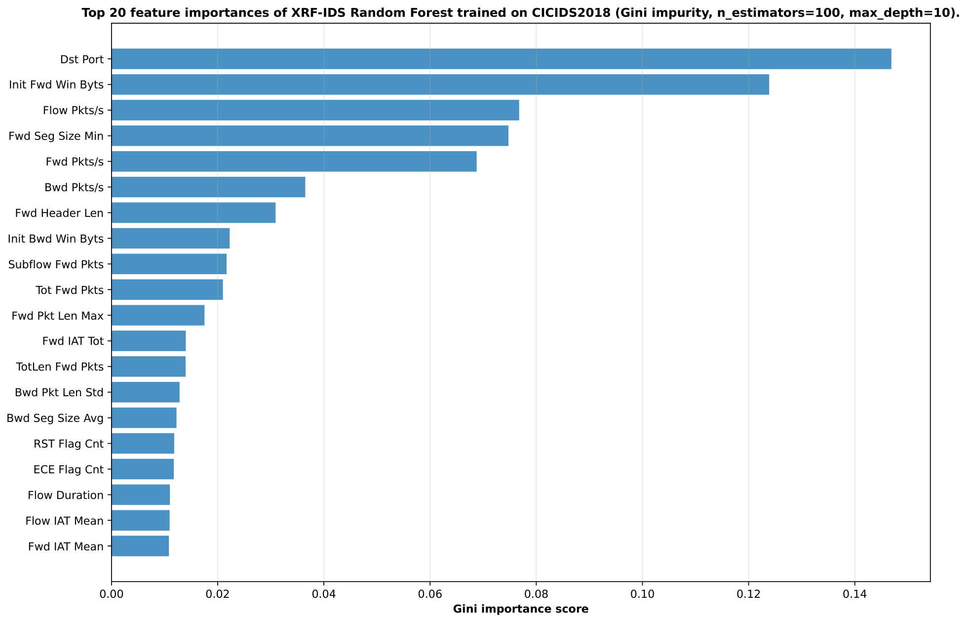
Importance was evaluated using the Mean Decrease in Gini Impurity of the trained RF ensemble over all 78 features of the CICFlowMeter. All 78 features were used to train the model and no explicit feature elimination was applied. According to Table 4, the first seven features sum to 55.85% of the cumulative importance, for interpretability characterization. Setting max_depth = 10 implicitly regularizes the RF classifier, thereby avoiding low-importance features at higher decision tree levels. Hence, Table 4 characterizes the feature relevance instead of reducing the number of training features. The most discriminative features were Dst Port (14.69%) and Init Fwd Win Byts (12.39%), with a cumulative total importance of 27.08%.

3.3. Model Training

3.3.1. Classifier Configuration

The RF classifier was trained using the following hyperparameters: n_estimators = 100 , max_depth = 10 , oob_score = True , n_jobs = 1 , and random_state = 42 . The constraint max_depth = 10 bounds each decision path to at most ten split conditions.

3.3.2. Class Weighting

Custom class weights address the severe class imbalance in Table 3 while preserving normal traffic recall. The fully balanced scheme (class_weight = ‘balanced’) was first evaluated and produced a Normal recall of 66.6%, which was operationally unacceptable. A custom-moderate scheme was subsequently designed: Normal 1.0 × , DoS/BruteForce 1.5 × , Botnet 2.0 × , and Infiltration 3.0 × . This restored Normal recall to 99.52 % while maintaining 97.57 % overall accuracy, at the cost of reduced Infiltration recall ( 32.14 % )—a deliberate trade-off favoring low false-positive volume (Section 4.1.4). The Infiltration class, which corresponds to the reconnaissance phase of an attack, receives the highest weight because of its high similarity to normal traffic. The Botnet class has a high weight because it has an imbalance ratio that is four times that of the normal traffic. The DoS/BruteForce classes received relatively moderate weights because both classes had comparatively balanced proportions.

3.3.3. Validation Protocol

The performance was assessed using the following criteria: (i) OOB score on the training partition, (ii) five-fold stratified cross-validation reporting the mean accuracy and 95% CI, and (iii) a held-out test partition of 648,759 flows reserved for the final evaluation.

3.4. Domain-Transfer Retraining Procedure

Cross-dataset evaluation follows a combined-data retraining procedure rather than a formal target-domain retraining algorithm (e.g., feature-space alignment or adversarial domain-invariant training); this distinction is stated explicitly here to avoid overstating the sophistication of the method. For a given adaptation budget b % , b % of the labeled target-domain flows (NF-ToN-IoT-v3 or NF-UNSW-NB15-v2) are randomly sampled (stratified by binary label) and appended to the full CSE-CIC-IDS2018 source training partition. A new Random Forest is then trained from scratch on this combined source-plus-target set, using the same hyperparameters ( T = 100 , max _ depth = 10 ) as the source-only model, and evaluated on the remaining, held-out target-domain flows. Because the source and target datasets use structurally incompatible feature extractors (CICFlowMeter vs. NetFlow/nProbe), evaluation is restricted to the binary Benign/Attack taxonomy shared by both (Section 4.6). For the active-learning variant, the b % target-domain sample is selected by predictive uncertainty (lowest classifier margin) rather than at random, reducing the number of flows an analyst must label to reach the same adaptation budget.

3.5. Explainability Engine: Path-Gini Selection (PGS)

We present PGS, a per-instance explanation mechanism that approaches the standard RF prediction call and involves no computation beyond the classification forward pass. Whereas SHAP [14] and LIME [13] offer post hoc explanations that require further model evaluations, and the previously proposed rule extraction approaches [20,21] rely on ranking the paths based on a population-wide analysis along with additional computations for each sample, PGS operates per instance at inference time through a precomputed leaf-level lookup, adding no inference overhead while providing determinism and verifying ensemble fidelity beyond the standard prediction call.

3.5.1. Per-Decision Explanation

For each classified flow x , three quantities were computed using the standard RF prediction routine.
  • Per-tree vote probability:
v t ( x ) = n t ( x ) y ^ n t ( x )
where t ( x ) is the leaf reached by x in tree t; n t ( x ) y ^ is the training sample count of the predicted class at that leaf; and n t ( x ) denotes the total training sample count at that leaf.
  • Ensemble confidence:
p ^ ( x ) = 1 T t = 1 T v t ( x )
  • Path-Gini score:
G t ( x ) = 1 d t ( x ) k = 1 d t ( x ) Gini ( n k )
where d t ( x ) is the depth of leaf t ( x ) and Gini ( n k ) is the Gini impurity at node k along the root-to-leaf path.
Each splitting node of a decision tree is assigned a Gini measure of impurity indicating the extent to which the samples used in the training are mixed; a score near zero indicates that nearly all samples belong to one class, and the model is confident in that node. A high score suggested high mixing between classes, implying that this split offered little separation from the main body. By computing the mean value of these measures across the entire path from the root to a leaf, G t ( x ) captures how consistently the tree copes with the incoming flow at each stage rather than only in the final stage of the path. A tree can reach a high-confidence leaf despite passing through uncertain intermediate nodes, because a strong final split can compensate for earlier weak ones; leaf confidence alone does not capture this path-level uncertainty. The mean path-Gini score instead rewards trees that are clear and decisive throughout the entire path, making it a better indicator of which tree genuinely understood the flow than which tree happened to end confidently. The representative decision path is taken from the tree t * = arg min t G t ( x ) . PGS is implemented as a precomputed lookup: at the training time (0.13 s, performed once), the average path-Gini score for every leaf in every tree is computed and stored in a lookup array of shape ( T , max _ nodes ) . At inference, rf_model.apply(X) retrieves leaf indices for all T trees in a single C-level call, precomputed scores are retrieved via a single NumPy gather operation, and "argmin" selects the explanation tree with zero Python loops during inference. This reduces the per-sample explanation cost from O ( T · d ) Python loop iterations to O ( T ) NumPy operations, achieving a 20.9× speedup over the naive Python implementation of PGS itself and a separate gain from the 460 470 × latency advantage over SHAP, detailed in Section 3.5 below, which compares PGS with post hoc explanation methods.

3.5.2. Path-Selection Strategy Comparison

To validate the PGS criterion, four path-selection strategies were evaluated on the full CSE-CIC-IDS2018 hold-out test partition ( n = 648,759 flows, Table 5). The Most Confident Tree (MCT) strategy selects the tree with the highest leaf confidence independent of the ensemble prediction. The Shortest Path Tree (SPT) strategy selects a tree with fewest decision nodes. The Random Tree (RT) strategy provides a lower-bound baseline. The PGS achieved 99.36% overall fidelity, outperforming MCT (98.01%), SPT (97.60%), and RT (98.11%). The advantage was most pronounced for the Infiltration class (91.34% vs. 83.23% for MCT and 89.98% for SPT on 20,539 Infiltration test flows), confirming that path-level purity is a more reliable selection criterion than leaf-level confidence for ambiguous minority-class flows.

3.5.3. Threshold Inverse Operationalization (TIO)

Previous approaches such as RDTIDS [20] and inTrees [21] have mentioned split thresholds within the normalized feature space used for training resulting in conditions such as Flow Pkts/s > 0.73, which cannot be directly validated against the network dashboard owing to the lack of automatic conversion in the deployment processes [16]. TIO fills this gap by automatically converting each split threshold back to its original network unit at rule generation time,
x raw = x norm · ( x max x min ) + x min
where x max and x min are the training partition extremes for each feature, computed only once during training and reused when generating rules without adding any inference overhead. The key point here is not the inversion equation itself, a regular min–max inverse, but rather its consistent integration into the process of rule generation. The reconstructed threshold values are fed to the TTOL to assign them the appropriate tier and generate the versioned output, resulting in each rule being expressed using verifiable values, such as pkt/s packet rates and μs without requiring further post-processing.

3.5.4. Latency Benchmarking

Explanation latency was measured over 10 independent timing trials of a fixed 1000-flow batch, with per-flow latency computed by dividing each trial’s total batch time by 1000, using time.perf_counter(); mean, standard deviation, and 95% confidence intervals across the 10 trials are reported for each method. RF prediction alone (no explanation overhead) is included as a baseline. SHAP TreeExplainer was evaluated using default parameters. The LIME tabular explainer uses 5000 perturbation samples for each instance. The results are presented in Table 6.

3.6. Rule Extraction and Management

Two additional mechanisms complement TIO (Section 3.5.3): SWCS and TTOL, which transform the raw ensemble decision paths into SOC deployable artifacts. As discussed in Section 2.2 (intrinsic interpretability approaches), prior rule-extraction systems address candidate generation and ranking but report normalized thresholds and provide no operational lifecycle management.

3.6.1. Rule Extraction

Every root-to-leaf path in every tree is a candidate IF-THEN rule. For T = 100 trees with max_depth = 10 , the candidate pool contained a maximum of T · 2 10 = 102,400 rules. Each rule r i is described by the condition set C i and confidence c ^ i , the fraction of training samples at the leaf belonging to the predicted class, and support s i , the absolute training sample count at the leaf node.

3.6.2. Support-Weighted Confidence Score (SWCS)

The rules were ranked according to their quality scores.
Q i = c ^ i · log ( 1 + s i )
This log-support-weighted confidence score penalizes single-sample overfitted paths while rewarding high-coverage, high-confidence patterns, a novel ranking criterion relative to the frequency or confidence-only ranking in previous frameworks [20,21].

3.6.3. Three-Tier Operational Lifecycle (TTOL)

Rules are assigned to one of the three tiers based on confidence and support:
  • Tier 1 (auto-deployment): c ^ i 0.95 and s i 10 . The rules are exported in IF-THEN format with raw-unit thresholds from (4).
  • Tier 2 (analyst review): 0.85 c ^ i < 0.95 or 1 s i < 10 . The rules were queued for manual validation prior to deployment.
  • Tier 3 (diagnostic): c ^ i < 0.85 . These rules were retained for diagnostic purposes only.
After each retraining cycle, the rules are versioned and archived for audit purposes, whereas such a lifecycle framework is absent from prior extraction systems.

3.6.4. Rule Export and SOC Deployment

The TTOL lifecycle includes a rule export module that translates the XRF-IDS IF-THEN conditions into deployment-ready formats. TIO ensures that all thresholds are in raw network-observable units prior to export, eliminating the manual back-transformation required by RDTIDS [20] and inTrees [21]. Table 7 illustrates the translation of a representative Tier-1 DoS rule into Snort and Suricata formats.
TTOL tier assignment maps to SIEM severity levels: Tier-1 is pushed as an automated signature; Tier-2 is queued for analyst review; and Tier-3 generates diagnostic log entries without active blocking.
The Snort and Suricata rules in Table 7 are templates, not exact semantic equivalents of the flow-level IF-THEN condition. CICFlowMeter features are computed as aggregates over a completed flow (e.g., Fwd_Pkt_Len_Max is the maximum forward packet length across all packets in the flow), whereas Snort and Suricata inspect traffic at the packet level in real time and lack native access to full-flow aggregates without additional flow-tracking infrastructure (e.g., Zeek/Bro flow logs or Suricata’s flow-scripting capabilities). The illustrated rules therefore approximate the detection intent using each engine’s available packet-level and count-based primitives; exact operationalization requires either flow-level preprocessing upstream of the signature engine or a dedicated flow-aware rule syntax and is identified as an engineering direction for future work.
Independently of the signature-engine syntax, the rule’s decision equivalence with the source model was validated directly: the three flow-level conditions were applied to the full held-out test partition ( n = 648,759 flows, independent of the training data used to compute the rule’s leaf-level confidence and support). Of the 92,186 flows satisfying all three conditions, 80.83 % receive the same DoS classification from the full Random Forest ensemble, and 80.73 % carry the true DoS label. This independently measured decision fidelity is lower than the rule’s leaf-level confidence ( c ^ i = 0.998 , Table 7), which reflects local purity within a single tree computed on training data; the two are distinct quantities, and the former is the more representative estimate of the rule’s standalone reliability as a simplified decision procedure applied outside the full ensemble structure. Full live integration testing is identified as future work.

3.7. MITRE ATT&CK Mapping Definition

A deterministic feature-conditioned function maps each predicted attack class to a MITRE ATT&CK tactic. This attribution approach (G3, Section 1) was implemented as described below. All thresholds are expressed in raw network units using (4).

3.7.1. Implemented Mappings

Four attack-to-ATT&CK mappings correspond to four attack classes:
  • DoS → Impact (TA0040)/Network DoS: Direct Network Flood (T1498.001). Conditions: Flow Pkts/s > 10,000 and Flow Duration < 1000 ms.
  • BruteForce → Credential Access (TA0006)/BruteForce (T1110.001). Conditions: Fwd Pkts/s > 1000 and Flow Duration < 1000 ms.
  • Botnet → Command and Control (TA0011)/Application Layer Protocol (T1071.001). Conditions: Flow Duration > 500 ms and Flow Pkts/s > 300 .
  • Infiltration → Initial Access (TA0001)/Exploit Public-Facing Application (T1190). Conditions: Flow Duration > 30,000 ms and Flow Pkts/s < 50 .
Normal Traffic Did Not Receive ATT&CK Attributions
Each mapping is justified against the corresponding MITRE ATT&CK technique definition and the dominant network-observable behavior of the underlying CSE-CIC-IDS2018 attack subtypes (Appendix A). BruteForce and Botnet map to single, behaviorally homogeneous subtypes (credential-stuffing floods and C2 beaconing, respectively), for which the assigned technique is representative of the great majority of class instances. DoS and Infiltration are more heterogeneous: the DoS class merges both volumetric flooding subtypes (LOIC, HOIC) and application-layer, deliberately low-rate subtypes (Slowloris, SlowHTTPTest, Hulk, GoldenEye), of which only the former exhibits the high-packet-rate signature associated with T1498.001 (Direct Network Flood); the assigned technique should therefore be read as representative of the class’s dominant or defining behavior rather than uniformly applicable to every instance. This is a class-to-technique design mapping, not an instance-level, expert-validated attribution: no independent domain-expert annotation was performed, and inter-rater agreement is therefore not applicable. Instance-level attribution, ideally validated by multiple independent analysts against ground-truth technique labels, remains an important direction for future work.

3.7.2. Mapping Evaluation

The tactic-level and technique-level correctness were verified as the fraction of correctly assigned labels over all true-positive detections in the test partition, with results for each class reported in Section 4.

3.8. SCAFP: Adaptive Feedback Loop

We introduce SCAFP, which simultaneously models the three explicit SOC operational constraints. As discussed in Section 2.4, prior adaptive feedback protocols lack realistic SOC constraints and formal statistical validation. SCAFP models: (i) analyst label noise ( η = 8 % ); (ii) delayed review rounds ( δ = 30 % ), reflecting documented SOC alert-fatigue and analyst-capacity constraints under which a substantial share of scheduled reviews are missed, postponed, or deprioritized [42]; and (iii) a bounded weekly correction budget ( ρ = 10 % ), representing a conservative fraction of the false-positive backlog reviewable within typical SOC analyst capacity, where analysts report spending up to a quarter of their time processing false positives alone [42]. These baseline values are illustrative operating points rather than precise empirical estimates derived from a single unified study; their individual and joint influence is characterized directly through the 96-configuration sensitivity sweep spanning η [ 0 % , 20 % ] , δ [ 0 % , 50 % ] , and ρ [ 5 % , 20 % ] (Section 4.7), rather than relying on the baseline point alone.

3.8.1. Simulation Protocol

The simulation modeled a weekly SOC review cycle over 12 iterations. At each iteration k { 1 , , 12 } ,
  • The current model classifies all flows in the monitoring window.
  • A fraction ρ = 10 % of false-positive alerts is selected for the simulated correction.
  • Each correction is independently mislabeled with probability η = 8 % , drawn uniformly from the remaining classes.
  • A fraction δ = 30 % of rounds is skipped, modeling the missed review cycles.
  • Corrected samples are appended to the training set.
  • The RF was retrained from scratch. max_depth = 10 is preserved to maintain rule extractability.
The 12 iterations form the main evaluation framework and serve as the only input to all reported statistical tests, presented in Section 4. The ablation tests, presented in Section 4, are based on an independent 6-iteration evaluation using a subset of 50,000 flows selected from the data stratification to identify the contributions of single parameters under limited resources. The shorter horizon is sufficient for ablation purposes because the false positive rate trend stabilizes within four iterations across all tested configurations. Statistical significance claims (Wilcoxon signed-rank test, Mann–Whitney U test, and Spearman rank correlation coefficient) were based only on the results of 12 iterations. Relative importance claims are based on 6-iteration ablation and must not be mixed with statistical claims.

3.8.2. Ablation Configurations

Four configurations were used to isolate the effects of each parameter. Config. A (full): ρ = 10 % , η = 8 % , δ = 30 % ; Config. B (no noise): ρ = 10 % , η = 0 % , δ = 30 % ; Config. C (no delay): ρ = 10 % , η = 8 % , δ = 0 % ; Config. D (no feedback): ρ = 0 % , η = 8 % , δ = 30 % .

4. Experimental Results and Analysis

This section presents an evaluation of XRF-IDS across seven dimensions: in-domain detection performance, baseline comparison, SOC-compatible throughput and explainability, IF-THEN rule extraction, MITRE ATT&CK mapping, cross-dataset adaptation, and adaptive feedback loop effectiveness. For in-domain detection, the performance was measured via per-class precision, recall, F1-score, and false positive rate, using standard metrics computed against a held-out test set ( N = 648,759 flows). A one-vs-rest strategy was used in the multiclass ROC-AUC calculations. The five-fold cross-validation results included the mean accuracy and 95% CI ( x ¯ ± 1.96 σ / 5 ).

4.1. In-Domain Detection Performance

4.1.1. Overall Accuracy and Stability

Under a random, stratified i.i.d. -style split ( n = 648,759 flows, 30% held out), XRF-IDS achieved 97.57% test accuracy, with an out-of-bag (OOB) score of 97.55% ( Δ = 0.02 % ) [6]. A complementary temporal-split evaluation (Section 4.8) yields 89.13% accuracy; the latter reflects deployment on genuinely unseen future traffic rather than traffic drawn from the same time window as training, and constitutes the more operationally realistic generalization estimate of the two. The five-fold stratified cross-validation yielded 97.56 % ± 0.05 % (95% CI: [97.45%, 97.66%]), confirming stable performance across all training folds.

4.1.2. Per-Class Detection Metrics

The per-class AUC scores (one-vs-rest) are listed in Table 8, and the threshold sensitivity for the Infiltration class is discussed in Section 4.1.4.
Three distinct false-positive quantities are used across this manuscript. The one-vs-rest per-class FPR reported in Table 8 is defined, for a class c, as FPRc = (flows not truly c, predicted as c)/(total flows not truly c). Under this definition, the Normal row’s FPR = 0.0008 counts attack flows incorrectly predicted as Normal, relative to all actual attack flows. The operational IDS false-positive rate, used from Section 3.8 onward, counts truly-Normal flows incorrectly flagged as any attack class, relative to all Normal flows; this is the SOC-relevant alert-volume metric. The SCAFP FPR is identical in definition to the operational false-positive rate, tracked over the 12-week deployment simulation.

4.1.3. Confusion Matrix Analysis

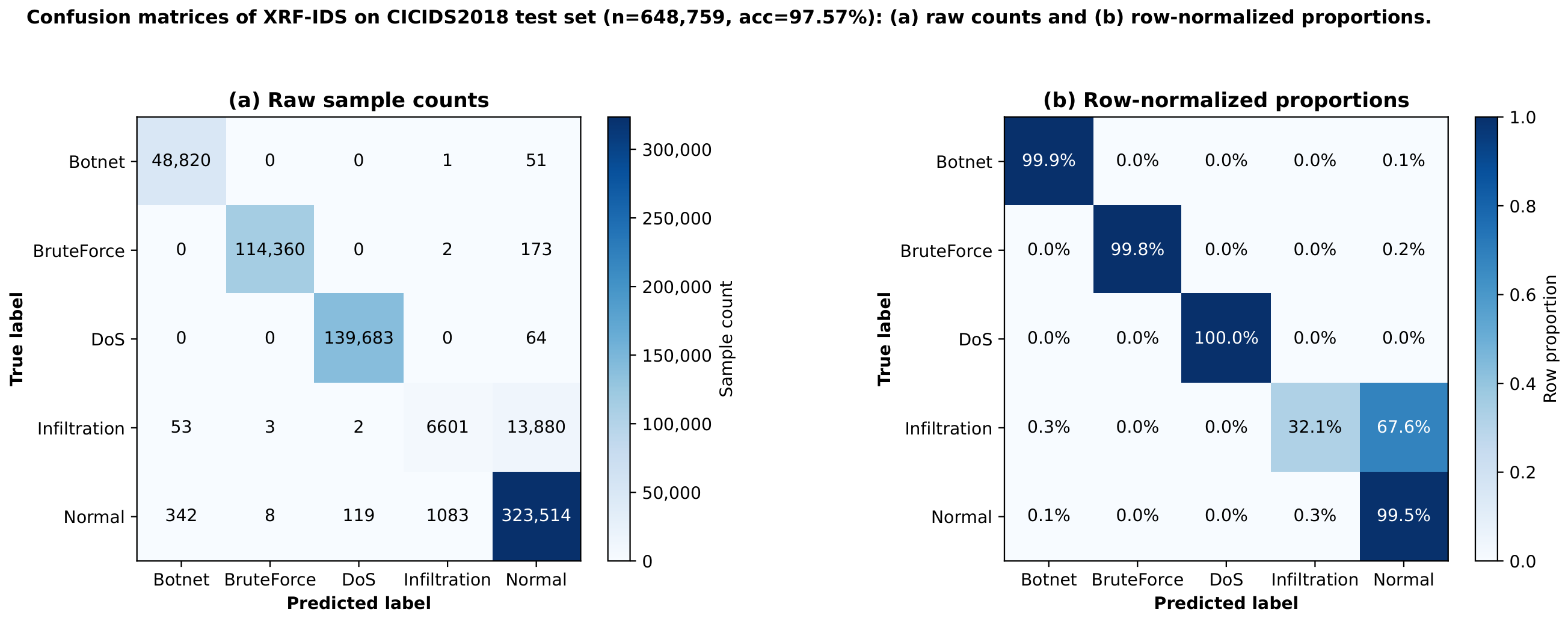
Off-diagonal concentrations are localized exclusively to the Infiltration row (Figure 2), where 67.6% of true Infiltration flows are misclassified as Normal, consistent with the single-packet probe profile documented in Appendix A.

4.1.4. Infiltration Class Analysis

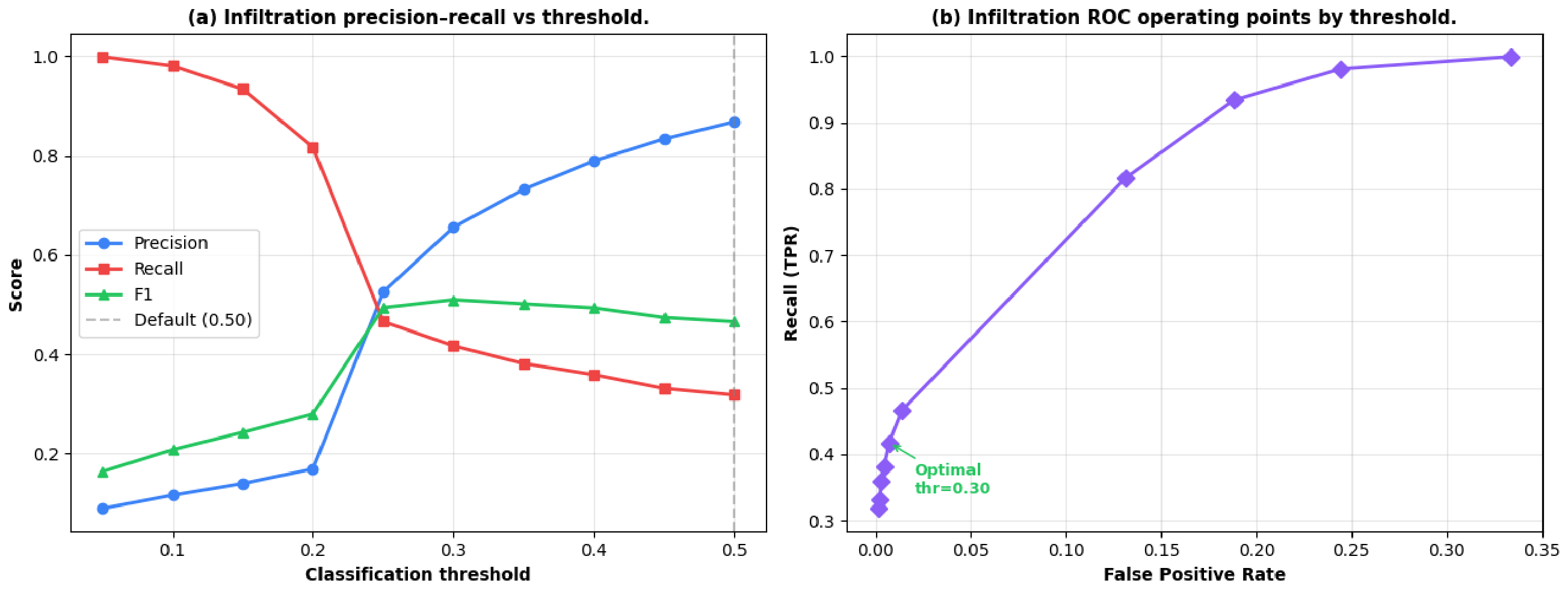
Threshold calibration was performed for the Infiltration class (Figure 3). At the default threshold ( τ = 0.50 ), Infiltration recall was 32.14% (Table 8). The threshold sweep (Figure 3a) shows recall increasing and precision decreasing as τ is lowered; the recommended operating point at τ * = 0.30 (Figure 3b) raises recall to 41.7% at a false positive rate of 0.72% (AUC = 0.9432 ), evaluated on the n Infiltration = 812 stratified test flows. For additional validation, the same operating point was re-evaluated on the full 648,759-flow hold-out partition ( n Infiltration = 20,539 , 25× larger), confirming Recall = 41.69 % and yielding F1 = 0.5097 (Precision = 0.6556 ) at 97.35% overall accuracy, consistent with the smaller-sample result and validated at substantially higher statistical power.
The threshold sweep reveals a sharp discontinuity between τ = 0.20 (Rec = 0.817 , FPR = 13.14 % ) and τ = 0.25 (Rec = 0.466 , FPR = 1.38 % ), indicating that approximately 40% of Infiltration flows receive posterior probabilities in the ambiguous range [ 0.20 , 0.25 ] where the model cannot assign a confident class decision. Lowering the threshold further to τ = 0.10 raises recall to 98.09% but collapses precision to 11.60% (F1 = 0.2075 , overall accuracy = 76.20 % ), generating approximately 133,000 false alarms on the test partition confirming τ = 0.30 as the optimal operating point. The class weight sweep confirms the same constraint: F1 peaks at weight = 7 × (F1 = 0.4968 ) and collapses at weight = 25 × (F1 = 0.2202 , overall accuracy = 78.05 % , Normal recall = 56.45 % ), generating 435 false alarms per 1000 legitimate flows and an operationally unacceptable false-positive volume [3]. The domain rule (Fwd_Pkt_Len_Max = 0 AND Tot_Fwd_Pkts = 1 ) adds zero improvement beyond τ = 0.30 threshold calibration, confirming that port scan probes and legitimate single-packet flows are statistically indistinguishable in the CICFlowMeter feature space.
The difficulty of detecting Infiltration is well documented in the literature. Cheng et al. [10] reported that DNN achieved F1 = 0 % and CNN achieves F1 = 4.73 % on the same CSE-CIC-IDS2018 dataset; XRF-IDS at τ = 0.30 is approximately 10 × better than the best published deep learning result on this class. Hajj et al. [29] excluded Infiltration entirely from their evaluation. Fernandes et al. [43] demonstrated that a dedicated LSTM combined with Tomek links and random undersampling still achieves a sensitivity = 0.82 for this class. Liu et al. [44] documented errors throughout the CSE-CIC-IDS2018 creation lifecycle, including attack orchestration, feature generation, and labeling. Goldschmidt and Chudá [12] identified Infiltration under-representation as a primary benchmark limitation. An AUC of 0.9432 confirmed that XRF-IDS correctly ranked Infiltration flows above Normal in 94.32% of the cases, but the decision boundary could not be crossed cleanly without generating operationally unacceptable false-positive volumes. XRF-IDS does not purport to be a complete Infiltration detection solution; resolution requires inter-flow temporal features from flow sequences grouped by source IP, identified as the primary future direction.

4.1.5. Feature Importance Analysis

Figure 4 shows the top-20 Gini importance scores. The two highest-ranked features were Dst Port (14.69%) and Init Fwd Win Byts (12.39%), which jointly accounted for 27.08% of cumulative importance. Port-based discrimination is evident in the feature importance ranking: DoS targets port 80, BruteForce targets port 22, and Botnets use a non-standard high port.The initial window-byte size discriminates between Botnets (small window, ≤32,737 B) and DoS (large window, >26,722 B). Packet rate and header-length features collectively capture volumetric and connection-setup signatures that differentiate BruteForce from Normal and Infiltration from Normal at finer granularities [2,5].

4.2. Baseline Model Comparison

Table 9 compares XRF-IDS against six baselines on the same hold-out set: Decision Tree (max_depth = 10 ), XGBoost, LightGBM, RF + SMOTE, RDTIDS proxy [20] (Decision Tree at depth 6, re-implementing the methodology of [20]), and inTrees proxy [21] (RF path extraction on the full 648,759-flow hold-out partition, re-implementing the methodology of [21]). XRF-IDS achieved the highest accuracy (97.57%) and macro precision (0.9704). The Decision Tree baseline at identical depth yields 80.75% accuracy (a 16.82 pp gap), confirming that the RF ensemble provides substantial accuracy gains over a single interpretable tree, while XRF-IDS recovers single-tree interpretability through PGS path selection.

4.3. SOC-Compatible Throughput and Explainability Latency

4.3.1. End-to-End Latency and Throughput

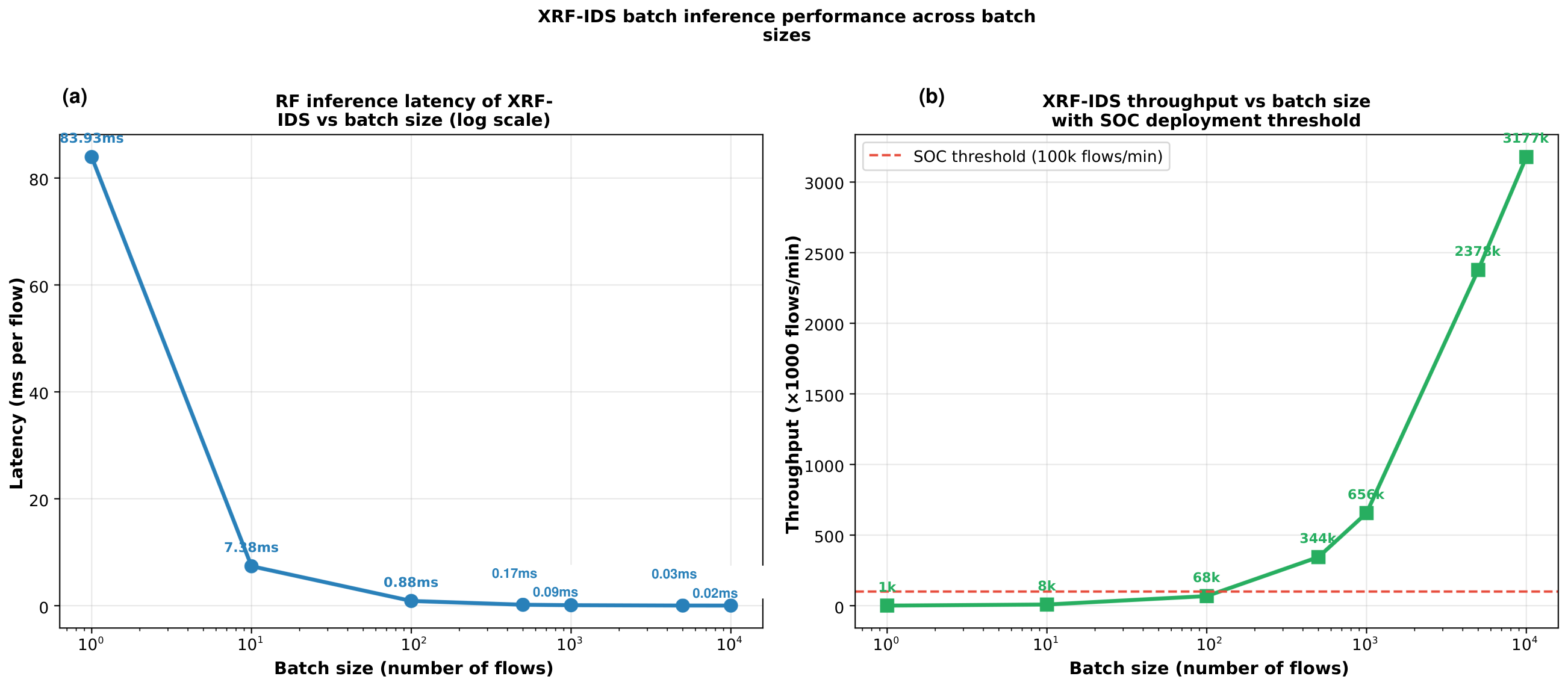
XRF-IDS achieved a maximum throughput of 3,177,431 flows/min at a batch size of 10,000, which was approximately 32 times higher than the SOC threshold [3] (Figure 5). Throughput exceeded 100,000 flows/min for all batch sizes from 500 onward. This throughput measurement covers the RF classification step only and does not include upstream feature extraction latency (CICFlowMeter: approximately 50–200 ms per flow depending on hardware), log ingestion, alert enrichment, or SIEM integration overhead. End-to-end SOC pipeline profiling is identified as a future evaluation priority.

4.3.2. Explainability Latency Comparison

Table 6 quantifies the latency and throughput advantage of PGS over SHAP and LIME. Beyond throughput, PGS provides four structural properties absent from post hoc methods: (i) deterministic per-instance explanations: identical inputs always produce identical outputs [16]; (ii) a 99.36% empirical ensemble fidelity, verified on the full 648,759-flow hold-out partition (Table 5), with disagreements flagged for analyst review; (iii) raw-unit threshold conditions: TIO reconstructs thresholds in raw network units (port numbers, pkt/s, μs) that map directly to firewall rules without post-processing [16]; and (iv) zero inference overhead: the 0.13 s precomputation occurs once at training time. Concurrent multithread workload testing and end-to-end integration with a live SIEM pipeline have not yet been performed and are identified as the primary future evaluation directions.

4.4. IF-THEN Rule Extraction Quality

The generation of rules via the SWCS and TTOL, starting from the customized RF_rules model, resulted in 8865 candidate rules for four attacks (Botnet, BruteForce, DoS, and Infiltration). The DoS rules had the highest mean support value because of their volumetric and high-rate flooding nature, whereas the Infiltration rules have the lowest mean support value because of their low volume and stealthy attack nature. After filtering based on the quality scores (5) and deduplication of conditions, 500 rules were selected to be unique in structure. TTOL assignment resulted in 499 Tier-1 rules (confidence 0.95 , support 10 ), one Tier-2 analyst-review rule, and zero Tier-3 diagnostic-only rules. A large number of Tier-1 rules indicate high separability of CSE-CIC-IDS2018 according to the defined thresholds, and datasets with lower separability result in balanced TTOL assignments [6]. The 499 Tier-1 rules have an average confidence of 98.7% and an average support of 27,413 training samples, while their average complexity is 9.5 ± 1.2 , consistent with max_depth = 10. Coverage analysis showed that the top 20% of rules (100 rules) accounted for 25.3% of attack detections at a 99.2% mean confidence [1].

4.5. MITRE ATT&CK Mapping Implementation Check

Table 10 presents an implementation correctness check. The class-to-technique mapping is defined a priori in Section 3.7 using signatures derived from training-partition feature ranges (Appendix A); the table confirms that the deterministic function correctly implements this pre-defined mapping without a lookup or logic error. Independent, instance-level expert validation of the mapping’s semantic accuracy, ideally with inter-rater agreement across multiple analysts, is identified as future work. The rationale for each mapping, including the class-level heterogeneity of DoS and Infiltration, is detailed in Section 3.7. Beyond correctness, this mapping is also unlike other attempts to integrate ATT&CK into the security process pipeline [24] that require annotation of pre-existing signatures offline and techniques such as [22,23] that require knowledge graph lookups at an average execution time of 100–200 ms per flow. XRF-IDS performs attribution within the classification forward pass in sub-microseconds of overhead without external knowledge sources or unstructured inputs. Specifically, the mapping latency of XRF-IDS is <1 μs per flow, repeatedly measured, which is three orders of magnitude faster than that of knowledge graph [22] (100–200 ms) and text-based [23] (requires unstructured inputs unavailable from raw flow records) methods. A feature-conditioned refinement rule additionally reclassified 3.2% of the BruteForce detections based on Fwd Pkts/s exceeding 10,000 pkt/s, correctly reassigning all to the impact tactic (TA0040) and demonstrating extensibility. This evaluation covers four kill-chain phases, and broader validation across the full ATT&CK taxonomy is left for future research [3].

4.6. Cross-Dataset Adaptation

4.6.1. Domain Gap and Adaptation Efficiency

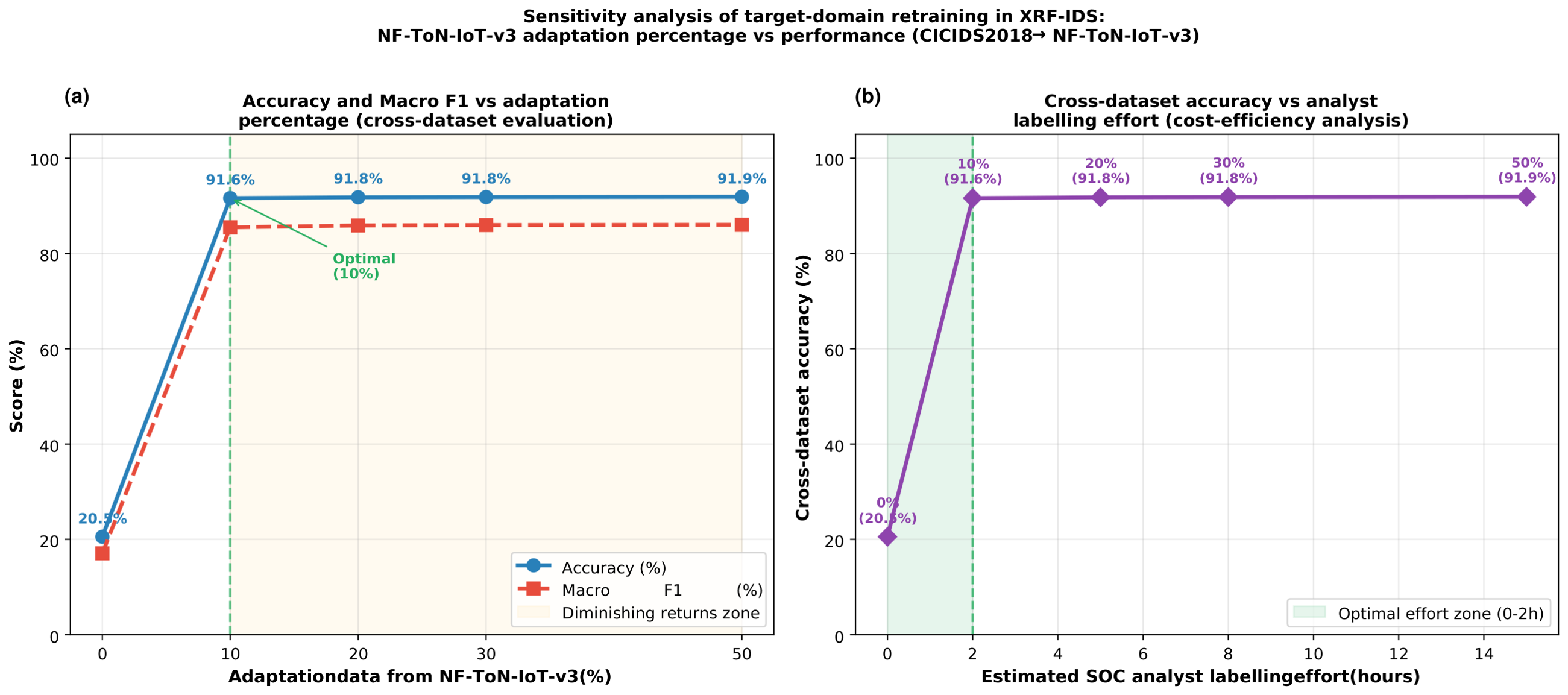
The experimental conditions are presented in Table 11; the combined-data retraining procedure is described in Section 3.4. Cross-dataset evaluation uses binary (Benign/Attack) classification to bridge the incompatible class taxonomies of CSE-CIC-IDS2018 and NF-ToN-IoT-v3, with 91.6% representing a conservative lower bound, as WebAttack and Reconnaissance misclassifications were counted as errors [11]. The direct transfer condition achieved 20.5% accuracy on NF-ToN-IoT-v3, confirming the well-documented domain gap between CICFlowMeter and NetFlow/nProbe extractors [6,14]. Target-domain retraining with 10% labeled NF-ToN-IoT-v3 flows (≈39,005 samples) achieved 91.6% accuracy and a gain of 71.1 pp. The zero-shot evaluation on NF-UNSW-NB15-v2 achieves 94.66% overall accuracy but Attack F1 = 0.002 (Table 12), an apparent contradiction explained by class imbalance: with 3.78% attack prevalence, a classifier predicting all flows as Benign achieves 96.22% accuracy. The near-zero Attack F1 confirms that the model identifies no attacks in the zero-shot mode and that the overall accuracy is a misleading metric in this imbalanced setting.

4.6.2. Adaptation Sensitivity Analysis

Accuracy and macro F1 rose sharply between 0% and 10% adaptation data, and then plateaued with marginal improvements of 0.3 pp between 10% and 50% (Figure 6). At 200–500 binary triage decisions per hour, a 10% adaptation budget requires approximately 78–195 h of analysis. The active learning selection of the 3,900 most uncertain flows reduces this process by approximately 8 h. These results identified 10% as the optimal operating point, maximizing the accuracy per analysis hour [2,6]. This diminishing-return characterization is not available for any single-condition cross-dataset evaluation in the reviewed literature. For the NF-UNSW-NB15-v2, five independent seeds were evaluated for each budget. On average, the cost-optimal point is 0.50% adaptation (10,000 flows, mean Attack F1 = 0.9205 ± 0.0048 ); however, this optimum is not consistent across all five seeds individually. The per-seed optima range from 0.25% to 1.01%, and the result should therefore be interpreted as mean-optimal rather than universally optimal. The decrease in mean Attack F1 from 0.50% to 1.01% ( Δ = 0.0002 < σ = 0.0048 ) falls within one standard deviation and is not statistically significant. In contrast, the further decline to 1.89% ( 0.9205 0.9149 , Δ = 0.0056 ) exceeds the standard deviation observed at 1.89% ( σ = 0.0014 ) and constitutes a real, statistically distinguishable effect: beyond the cost-optimal budget, additional NF-UNSW-NB15-v2 samples begin to overfit the combined training set toward the target-domain feature distribution, mildly displacing the CSE-CIC-IDS2018 source representation rather than continuing to close the residual domain gap [11].

4.7. Adaptive Feedback Loop Results

4.7.1. Performance Evolution and Statistical Significance

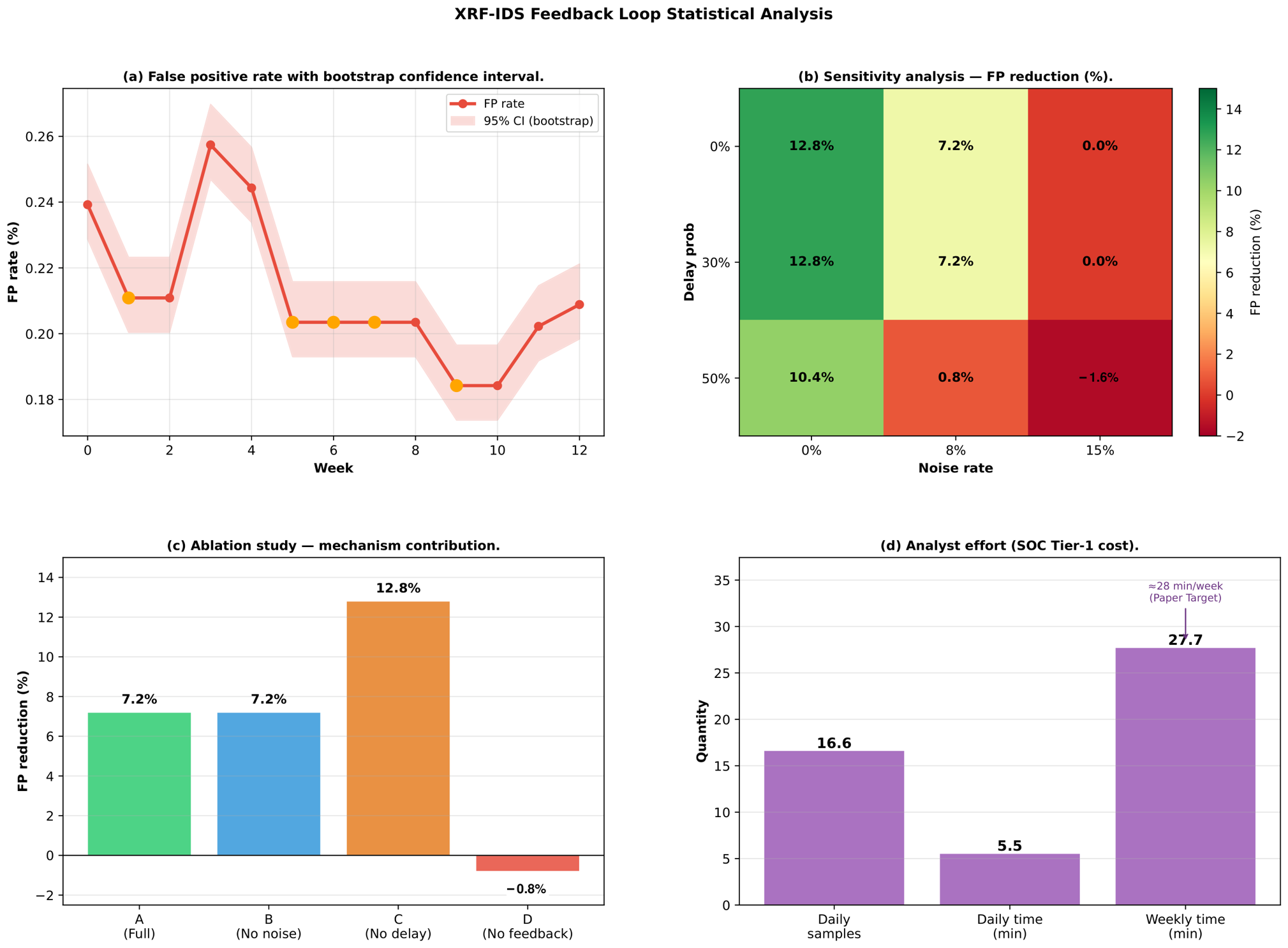
Figure 7 presents the evolution of the accuracy, false-positive rate, and false-negative rate over the 12-iteration simulation under the full SCAFP constraint model (Section 3.8). The FPR values at each iteration were computed over the monitoring-window partition used during the iteration’s simulated deployment cycle, not over the static held-out test partition reserved for in-domain evaluation. The two partitions were drawn from the same CSE-CIC-IDS2018 distribution but were independently evaluated to preserve the integrity of the test set. The FNR decreased from 2.185 to 2.175% over the same period. The total SCAFP analyst effort comprises 998 corrections across 12 iterations (≈83 per iteration; ≈28 min/week at 20 s/decision) [1,3].
Table 13 presents three non-parametric tests applied to the FPR trajectory across the 12 feedback iterations (weeks 1–12; week 0 is the pre-feedback baseline and is excluded from this comparison). The Mann–Whitney U test used in earlier analysis assumes independent samples, an assumption violated by the sequential, model-retraining structure of the weekly simulation; it is replaced here with the Mann–Kendall trend test, which is appropriate for time-ordered, dependent observations. All three tests are individually significant at the uncorrected α = 0.05 level; however, a Bonferroni correction for three tests ( α = 0.05 / 3 = 0.017 ) shows that only the Spearman trend correlation survives ( r = 0.70 , p = 0.011 ). The 12-week horizon was chosen to approximate a standard quarterly SOC review cycle for a proof-of-concept deployment; it necessarily limits the statistical power available to detect anything beyond a moderate-to-large effect. This is reflected directly in the results: the Wilcoxon signed-rank effect size is small (rank-biserial correlation = 0.095 ), and a bootstrap 95% confidence interval on the first-half-versus-second-half FPR difference is [ 0.001 , 0.049 ] percentage points, consistently positive, confirming the direction of the reduction, but narrow and close to zero at the lower bound, which is the expected signature of a small sample rather than evidence against a real effect. These results should therefore be read as an indicative, first-pass characterization of SCAFP’s effectiveness rather than a high-power confirmatory test. We interpret these results cautiously: the downward FPR trend over the 12-week deployment simulation is statistically supported by the Spearman trend correlation, which does not require the independence assumption violated by the sequential simulation structure and remains significant after correction for multiple comparisons. The Wilcoxon and Mann–Kendall results are directionally consistent but are not treated as independent confirmatory evidence given this correction. Both the Wilcoxon and one-sample t-tests are conducted as one-sided tests (testing specifically for a decrease in FPR), justified by the mechanism’s design: SCAFP corrects confirmed false positives through analyst feedback, so the only scientifically plausible outcomes are a reduction in FPR or no effect; an increase is not a mechanistically plausible alternative. This directional hypothesis was specified prior to observing the results, rather than selected post hoc.
To address the single-simulation-run limitation noted above, the full 12-week deployment simulation was independently repeated five times with varying random seeds (Table 14). All five runs show a positive FPR reduction, ranging from 11.40 % to 17.20 % (mean 14.50 % ± 2.45 % , 95% CI [ 11.46 % , 17.54 % ] , entirely above zero). Within-run trend significance varies naturally across seeds: three of five runs individually reach significance at the uncorrected α = 0.05 level (Spearman p { 0.010 , 0.011 , 0.019 } ), while two do not ( p = 0.094 , p = 0.386 ), illustrating genuine run-to-run variability in a stochastic simulation with n = 12 per run. Treating each of the five independent runs as one observation, a one-sample t-test rejects the null hypothesis of zero reduction ( t = 13.25 , p = 0.0001 ); a non-parametric one-sample Wilcoxon signed-rank test yields p = 0.031 , the minimum p-value achievable by this exact test at n = 5 given that all five runs share the same sign. This between-run consistency, obtained from genuinely independent replicates rather than re-analysis of a single trajectory, provides stronger evidence for the direction of the effect than the single-seed analysis alone, while the modest n = 5 and the two non-significant within-run trends are acknowledged as remaining limitations.

4.7.2. Ablation Study

Table 15 presents results from a 6-iteration ablation conducted on a stratified 50,000-flow subsample, separate from the 12-iteration primary evaluation used for significance testing (Table 13). The reduced iteration count is sufficient to isolate the directional effect of each parameter; the 6-iteration horizon consistently captures the performance differential between configurations because FPR stabilization is observed within four iterations across all tested settings. Statistical significance claims in Table 13 are drawn from the full 12-iteration sequence and are independent of the ablation findings presented herein. Removing the label noise (Config. B) produces no measurable change, indicating that the 8% analyst error rate does not substantially impede convergence. Removing delays (Config. C) increases the FP reduction from 7.2% to 12.8% ( + 5.6 pp), identifying delayed analyst availability as the primary performance bottleneck [3]. Removing all feedback (Config. D) produces a slightly negative result ( 0.8 % ), confirming that analyst corrections are the causal drivers of FP improvement [2].

4.7.3. Extended Sensitivity Analysis

A 96-configuration sweep ( η { 0.00 , 0.05 , 0.08 , 0.10 , 0.15 , 0.20 } , δ {0.00, 0.15, 0.30, 0.50}, ρ { 0.05 , 0.10 , 0.15 , 0.20 } ) was conducted using prediction-level simulation on the full RF model evaluated over the static held-out test partition (baseline operational FPR = 0.24%, 1552 false-positive flows among the Normal-class test set). All 96 configurations yield positive FPR reduction (range: + 0.10 to + 0.44 pp), confirming SCAFP robustness across the full tested parameter space. This prediction-level sweep, which applies corrections directly to the static test-set predictions without model retraining, is distinct from the iterative, retraining-based simulation shown in Figure 7b, which spans a substantially larger effect range due to genuine model updates across iterations. At the most adverse retraining-based configuration ( δ = 0.50 , η = 0.15 ), the small number of iterations (six) combined with a 50% per-round chance of a missed review round means that few or no correction rounds may succeed by chance; the resulting FPR reduction at this cell is subject to substantially higher variance than at more moderate parameter settings and can occasionally fall near or below zero as a consequence of this variance rather than indicating that feedback is systematically harmful under these conditions. Budget ρ is the dominant parameter; label noise η has a secondary effect with a critical threshold near η = 0.10 ; and missed rounds δ have the smallest effect. The baseline FP trajectory (1552 → 1411 → 1284 → 1172 → 1070 → 976 → 884 → 809 → 809 → 741 → 741 → 741 → 677 flows) shows monotonic convergence.

4.8. Temporal Evaluation

To assess whether the random stratified split overestimated performance, a date-based evaluation was conducted. Flows from 14–16 February 2018 (Week 1: 3,133,873 flows) were used for training; flows from 20–28 February 2018 (Week 2: 10,948,944 flows) were used for testing. This temporal, generalization-oriented evaluation yields 89.13% accuracy, 8.44 pp below the random i.i.d.-style stratified split (97.57%, Section 4.1). Per-class analysis identifies three dataset-inherent causes: (1) Infiltration is absent from Week 1 by dataset design; (2) DoS sub-types differ structurally across weeks; and (3) BruteForce is near-absent in the test set (841 flows out of 10.9 million). These findings confirm that CSE-CIC-IDS2018 is scenario-stratified rather than temporally i.i.d.

5. Discussion

5.1. Interpretation of Detection Performance

The near-perfect F1 scores for Botnet, BruteForce, and DoS reflect alignment between their discriminative feature spaces and the depth-limited RF decision boundaries. As reported in Section 4.1.5, Dst Port and Init Fwd Win Byts together accounted for 27.08% of the ensemble importance, suggesting that max_depth = 10 acts as an inductive bias toward promoting discriminative features into the higher depths of the decision trees, a process that would otherwise be undermined by greater depths or retrospective attributions.
The modest recall for Infiltration reflects an unavoidable feature-space overlap between reconnaissance probes (single-packet scans) and legitimate short flows, compounded by a deliberate design choice to prioritize low false-positive rates over maximizing detection for this rare class. As shown in Section 4.1.4, the model correctly ranks these flows (AUC 0.9432 ), but the decision boundary cannot be crossed cleanly without overwhelming SOC analysts with false alarms. This constraint is not unique to our approach; it has been independently documented by Cheng et al. [10], Hajj et al. [29], Fernandes et al. [43], and Goldschmidt and Chudá [12] on the same benchmark. Full resolution requires inter-flow temporal features (e.g., short-term source-IP sequences), which we identify as the primary direction for future work.

5.2. Significance of Intrinsic Explainability

The PGS latency advantage over SHAP and LIME (Table 6) is structural: its O ( T · d ) complexity bound matches the prediction call itself, ensuring that explanation throughput scales with classification throughput regardless of model size. In SOC deployments where explanations are required only for alerts (typically < 5 % of flows), the throughput gap narrows, but the three structural properties that matter for audit trails (determinism, empirically measured ensemble fidelity, and raw-unit threshold conditions) remain unavailable from post hoc methods regardless of volume [16].

5.3. Deployment Implications

As reported in Section 4.3, the system sustains throughput comfortably above the SOC minimum requirement while maintaining bounded O ( T · d ) per-sample complexity. Deployment coverage follows a similar pattern: 499 of the 500 extracted rules reach Tier-1 auto-deployment, with the top 20% accounting for 25.3% of attack detections at 99.2% mean confidence, though such high separability is unlikely to hold in more heterogeneous enterprise traffic [1].
SCAFP extends this static coverage over time: starting from a pre-feedback FPR baseline of 0.24% (Section 3.8), the single-seed simulation provides a 12.7% FPR reduction, and validation across five independent random seeds confirms a mean reduction of 14.50% (95% CI [ 11.46 % , 17.54 % ] ; Table 14). The ablation study results (Table 15) show that the feedback delay is a key obstacle. When the delays were removed (Config. C), the FPR reduction increases from 7.2% to 12.8% (+5.6 pp), indicating that prompt analyst review is critical for performance improvement. Disabling label noise did not change the FPR. Thus, the consistency of weekly feedback from analysts appears to be more crucial than the precision of their annotations [1,3].

5.4. Cross-Target-Domain Retraining

The cross-dataset results used binary classification; the 20.5% direct-transfer and 91.6% adapted accuracy figures represent benign/attack discrimination. The explainability mechanisms specific to this work (PGS, TIO, SWCS, TTOL rule tiers, MITRE ATT&CK mapping) are defined around the five-class CSE-CIC-IDS2018 attack taxonomy and were not re-evaluated under cross-dataset binary adaptation; this evaluation is scoped to classification performance and adaptation efficiency only, and extending intrinsic explainability and MITRE-mapped rule extraction to the adapted binary classifier is identified as future work. The conservative evaluation strategy counts WebAttack and reconnaissance misclassifications as errors, making 91.6% of the lower bound on matched-class performance. Accuracy rises sharply from 20.5% to 91.6% with just 10% of labeled target-domain data, then plateaus, with only 0.3 pp of additional gain across the 10%–50% range despite sevenfold more analyst effort. Active learning reduces this to approximately 8 h [2,6]. These results suggest that XRF-IDS is better characterized as domain-adaptable than as domain-invariant. The practical implication is that deployment in a new network environment requires approximately 78–195 analyst-hours of binary triage effort before acceptable performance is recovered, which is a non-trivial upfront cost that must be weighed against the alternative of deploying a signature-based system requiring continuous manual rule maintenance. For NF-UNSW-NB15-v2, the practical recommendation of a 0.50% adaptation budget is derived from the mean across five seeds rather than from a budget that is optimal under every random sampling of the adaptation set; SOC operators should therefore treat 0.50%–1.01% as an effective operating range rather than a single precise value. The decline observed beyond 1.89% adaptation is attributed to overfitting of the combined training set toward the target-domain feature distribution, which is a known risk of naive sample concatenation in target-domain retraining that could be mitigated in future work through sample re-weighting or domain-adversarial regularization [11].

5.5. Limitations

Infiltration detection. Even after optimal threshold calibration ( τ * = 0.30 ), XRF-IDS detects fewer than half of Infiltration attacks (recall 41.7 % ). From an operational standpoint, this is a substantive limitation: a SOC relying solely on XRF-IDS would miss the majority of this category. The system should therefore be deployed with the explicit expectation that Infiltration requires a complementary detection layer. Full resolution demands richer feature representations than CICFlowMeter’s single-flow aggregates, specifically, inter-flow temporal context, which we prioritize as future work.
Benchmark diversity. CSE-CIC-IDS2018 was captured in 2018 under controlled testbed conditions. Encrypted traffic is excluded from the evaluation. The CICFlowMeter features include payload-based statistics that carry discriminative values for TLS-encrypted flows; however, this is outside the scope of the current evaluation.
MITRE ATT&CK mapping scope. The mapping experiment includes four attack classes, thereby serving as an implementation correctness check for the evaluated kill-chain phases, but not a statistical accuracy evaluation for all 193 techniques included in the taxonomy. Extension to other attack taxonomies based on knowledge graphs constitutes a promising future research path.
Simulation versus deployment. No SOC analysts participated in the study, and all feedback was simulated using the constraint model defined in Section 3.8. The SCAFP constraint model (Section 3.8) is grounded in reported SOC operational characteristics [1,3] but cannot capture real analyst behavior in terms of cognitive load, alert fatigue, or domain expertise variability. Therefore, the results should be interpreted as indicative of the potential of the mechanism under controlled conditions, pending validation with real SOC analysts.
Throughput evaluation scope. The throughput was evaluated using a single-process batch simulation model with dedicated hardware. Concurrent multi-thread workload performance and end-to-end pipeline latency, including SIEM integration, alert enrichment, and analyst notification overhead, were not measured and may differ from the reported batch-processing figures in production environments.
Temporal evaluation. A date-based evaluation yields 89.13% accuracy, with three dataset-inherent causes identified (Infiltration absent from training partition by design, DoS sub-type shift, and BruteForce near-absent in test). These findings confirm that CSE-CIC-IDS2018 is scenario-stratified by construction (each capture day executes a scripted, non-overlapping subset of attack types) rather than temporally i.i.d.
SOC pipeline scope. End-to-end SOC pipeline profiling including feature extraction, log ingestion, alert enrichment, rule deployment, and SIEM integration was not conducted within the scope of this study and was identified as a priority for future operational validation.
Adaptation budget seed-sensitivity. On NF-UNSW-NB15-v2, the recommended 0.50% adaptation budget is mean-optimal across five seeds but not optimal for every individual seed (per-seed optima span 0.25–1.01%). Practitioners should validate the adaptation budget on a held-out subset of their own target domain rather than relying solely on the single value reported here.
Online adaptive IDS methods. Hoeffding Trees, Adaptive Random Forest, and related streaming classifiers [26,27] update incrementally on each arriving flow without batch retraining, which is fundamentally different from SCAFP’s weekly analyst-driven retraining cycle. A controlled comparison is precluded by the static batch format of CSE-CIC-IDS2018, which does not preserve the original temporal ordering of flows required for a fair streaming evaluation. Furthermore, none of the surveyed streaming IDS methods generated deployable IF-THEN rules in raw network units, which is the primary operational contribution of XRF-IDS. A comparison with streaming baselines on a purpose-built streaming benchmark is identified as a priority for future work.

6. Conclusions

This paper presents XRF-IDS, a SOC-oriented prototype and framework built around a depth-limited Random Forest IDS with five specifically designed mechanisms (PGS, TIO, SWCS, TTOL, and SCAFP), validated under controlled experimental conditions rather than demonstrated as a deployable SOC solution. Together, these mechanisms address six operational challenges (G1–G6) not jointly addressed by any single previously surveyed system (Table 1). When evaluated on the CSE-CIC-IDS2018 dataset (2,162,527 flows, five classes), XRF-IDS achieved competitive detection accuracy while delivering explanations two orders of magnitude faster than SHAP, with empirically measured ensemble fidelity (99.36%), supporting the kind of audit trails a production SOC deployment would require, though not yet validated as such. The cross-dataset evaluation based on NF-ToN-IoT-v3 (2025) achieved 91.6% classification accuracy after only 10% target-domain retraining, and on NF-UNSW-NB15-v2 (2015) reached mean Attack F1 = 0.9205 ± 0.0048 at a 0.50% adaptation budget, averaged over five independent seeds. SCAFP decreased the FPR by a mean of 14.50% (95% CI [ 11.46 % , 17.54 % ] ) across five independently seeded 12-iteration deployment simulations, with all five runs showing a positive reduction (one-sample t-test, p = 0.0001 ). Each simulated weekly review cycle required approximately 28 min of analyst time; this figure is distinct from the smaller-scale ablation study (Table 15) used only to isolate individual parameter contributions. As detailed in Section 5, the following limitations remain: benchmark recency, ATT&CK mapping scope, simulation-based feedback validation, and seed-dependent variability of the NF-UNSW-NB15-v2 adaptation budget recommendation. Future work will focus on the evaluation of more recent benchmarks, encrypted traffic, and production validation using real SOC analysts.


Author Contributions

Conceptualization, S.B. and M.Z.; methodology, S.B.; software, S.B.; validation, S.B., M.Z., S.A. and A.B.; formal analysis, S.B.; investigation, S.B.; resources, M.Z.; data curation, S.B.; writing—original draft preparation, S.B.; writing—review and editing, M.Z., S.A. and A.B.; visualization, S.B.; supervision, M.Z., A.B. and S.A.; project administration, M.Z. All authors have read and agreed to the published version of the manuscript.

Funding

This research received no external funding.

Institutional Review Board Statement

Not applicable.

Informed Consent Statement

Not applicable.

Data Availability Statement

This study used the publicly available CSE-CIC-IDS2018 benchmark dataset [12] and the publicly available NF-ToN-IoT-v3 and NF-UNSW-NB15-v2 cross-dataset benchmarks [11]. No new data were created for this study. The implementation code for the proposed mechanisms (PGS, TIO, SWCS, TTOL, and SCAFP) is available from the corresponding author upon reasonable request.

Acknowledgments

During the preparation of this manuscript, the authors used Paperpal (https://paperpal.com, Cactus Communications) and Claude Sonnet 5 (Anthropic) to improve language clarity, grammar, and phrasing in the Introduction, Results, and Discussion sections. These tools were used solely for language editing of author-written text and were not used to generate scientific ideas, hypotheses, data, analysis, or conclusions. All AI-assisted text was reviewed, verified, and edited by the authors, who take full responsibility for the content of this publication.

Conflicts of Interest

The authors declare no conflicts of interest.

Abbreviations

The following abbreviations are used in this manuscript:
XRF-IDSeXplainable Random Forest Intrusion Detection System
IDSIntrusion Detection System
SOCSecurity Operation Center
MLMachine Learning
RFRandom Forest
OOBOut-of-Bag
XAIExplainable Artificial Intelligence
LIMELocal Interpretable Model-agnostic Explanations
SHAPSHapley Additive exPlanations
GDPRGeneral Data Protection Regulation
PGSPath-Gini Selection
TIOThreshold Inverse Operationalization
SWCSSupport-Weighted Confidence Score
TTOLThree-Tier Operational Lifecycle
SCAFPSOC-Constrained Adaptive Feedback Protocol
CVCross-Validation
FPRFalse Positive Rate
F1F1-score

Appendix A. Attack Pattern Characterization

This section briefly discusses the per-class network-observable signatures qualitatively used to derive the MITRE ATT&CK mapping thresholds in Section 3.7. Port-based and behavioral discrimination between classes is summarized in Section 4.1.5. The Infiltration class exhibits substantial feature overlap with normal traffic, contributing to elevated false negative rates and constituting a known challenge for this benchmark [12].

References

  1. Sharma, R.M.; Pillai, V.; Chandrasekaran, B.; Doss, L.; Sudha, K.; Kadumbadi, V. Enhancing network security: The role of deep learning and explainable AI in intrusion detection systems. In Proceedings of the 11th International Conference on Communication and Signal Processing (ICCSP), Melmaruvathur, India, 5–7 June 2025; pp. 452–457. [Google Scholar] [CrossRef] [Scilit]
  2. Çelik, A.F.; Sağlam, B.; Demirci, S. Developing explainable intrusion detection systems for the Internet of Things. In Proceedings of the 16th International Information Security and Cryptology Conference (ISCTürkiye), Ankara, Turkey, 18–19 October 2023; pp. 1–6. [Google Scholar] [CrossRef] [Scilit]
  3. Vielberth, M.; Böhm, F.; Fichtinger, I.; Pernul, G. Security operations center: A systematic study and open challenges. IEEE Access 2020, 8, 227756–227779. [Google Scholar] [CrossRef] [Scilit]
  4. Le, T.-T.-H.; Kim, H.; Kang, H.; Kim, H. Classification and explanation for intrusion detection system based on ensemble trees and SHAP method. Sensors 2022, 22, 1154. [Google Scholar] [CrossRef] [Scilit] [PubMed]
  5. Patil, S.; Varadarajan, V.; Mazhar, S.; Sahibzada, A.; Ahmed, N.; Sinha, O.; Kumar, S.; Shaw, K.; Kotecha, K. Explainable artificial intelligence for intrusion detection system. Electronics 2022, 11, 3079. [Google Scholar] [CrossRef] [Scilit]
  6. Cantone, M.; Marrocco, C.; Bria, A. Machine learning in network intrusion detection: A cross-dataset generalization study. IEEE Access 2024, 12, 144489–144508. [Google Scholar] [CrossRef] [Scilit]
  7. Nakıp, M.; Gelenbe, E. Online self-supervised deep learning for intrusion detection systems. IEEE Trans. Inf. Forensics Secur. 2024, 19, 5668–5683. [Google Scholar] [CrossRef] [Scilit]
  8. Golpayegani, R.; Gerl, S.; Smati, D. Bridging the gap between AI and explainability in the GDPR: Toward trustworthiness-by-design in automated decision-making. IEEE Trans. Technol. Soc. 2022, 3, 24–35. [Google Scholar] [CrossRef] [Scilit]
  9. Shtayat, M.M.; Hasan, M.K.; Sulaiman, R.; Islam, S.; Khan, A.U.R. An explainable ensemble deep learning approach for intrusion detection in industrial Internet of Things. IEEE Access 2023, 11, 115047–115061. [Google Scholar] [CrossRef] [Scilit]
  10. Cheng, H.-C.; Tsai, M.-H.; Yu, C.-H.; Lai, C.-Y. Network anomaly intrusion detection based on deep learning approach. Sensors 2023, 23, 2171. [Google Scholar] [CrossRef] [Scilit] [PubMed]
  11. Sarhan, M.; Layeghy, S.; Moustafa, N.; Portmann, M. NetFlow datasets for machine learning-based network intrusion detection systems. In Proceedings of the 10th International Conference on Big Data Analytics and Knowledge Discovery (DaWaK), Vienna, Austria, 22–24 August 2022; pp. 117–135. [Google Scholar] [CrossRef] [Scilit]
  12. Goldschmidt, P.; Chudá, D. Network intrusion datasets: A survey, limitations, and recommendations. Comput. Secur. 2025, 156, 104510. [Google Scholar] [CrossRef] [Scilit]
  13. Ribeiro, M.T.; Singh, S.; Guestrin, C. “Why should I trust you?”: Explaining the predictions of any classifier. In Proceedings of the 22nd ACM SIGKDD International Conference on Knowledge Discovery and Data Mining (KDD), San Francisco, CA, USA, 13–17 August 2016; pp. 1135–1144. [Google Scholar] [CrossRef] [Scilit]
  14. Lundberg, S.M.; Lee, S.-I. A unified approach to interpreting model predictions. Adv. Neural Inf. Process. Syst. 2017, 30, 4765–4774. [Google Scholar]
  15. Mehmood, T.; Raza, A.; Aleem, M.; Iqbal, M.; Bhatti, K. DRIFTNET-EnVACK: Ensemble-based intrusion detection with adaptive concept drift handling for network security. IEEE Access 2024, 12, 80020–80034. [Google Scholar] [CrossRef] [Scilit]
  16. Neupane, S.; Ables, J.; Anderson, W.; Mittal, S.; Rahimi, S.; Banicescu, I.; Seale, M. Explainable intrusion detection systems (X-IDS): A survey of current methods, challenges, and opportunities. IEEE Access 2022, 10, 112392–112415. [Google Scholar] [CrossRef] [Scilit]
  17. Arreche, O.; Guntur, T.; Roberts, J.; Abdallah, M. E-XAI: Evaluating black-box explainable AI frameworks for network intrusion detection. IEEE Access 2024, 12, 23954–23988. [Google Scholar] [CrossRef] [Scilit]
  18. Bora, R.P.; Terhörst, P.; Veldhuis, R.; Ramachandra, R.; Raja, K. SLICE: Stabilized LIME for consistent explanations for image classification. In Proceedings of the IEEE/CVF Computer Vision and Pattern Recognition Conference (CVPR), Seattle, DC, USA, 17–21 June 2024; pp. 10988–10996. [Google Scholar] [CrossRef] [Scilit]
  19. Mohale, V.Z.; Obagbuwa, I. A systematic review on the integration of explainable artificial intelligence in intrusion detection systems to enhancing transparency and interpretability in cybersecurity. Front. Artif. Intell. 2025, 8, 1526221. [Google Scholar] [CrossRef] [Scilit] [PubMed]
  20. Ferrag, M.A.; Maglaras, L.; Ahmim, A.; Derdour, M.; Janicke, H. RDTIDS: Rules and decision tree-based intrusion detection system for Internet-of-Things networks. Future Internet 2020, 12, 44. [Google Scholar] [CrossRef] [Scilit]
  21. Deng, H. Interpreting tree ensembles with inTrees. Int. J. Data Sci. Anal. 2019, 8, 277–287. [Google Scholar] [CrossRef] [Scilit]
  22. Rafiey, P.; Namadchian, A. Mapping vulnerability description to MITRE ATT&CK framework by LLM. Adv. Artif. Intell. Mach. Learn. 2025, 5, 243. [Google Scholar] [CrossRef] [PubMed]
  23. Orbinato, V.; Barbaraci, M.; Natella, R.; Cotroneo, D. Automatic mapping of unstructured cyber threat intelligence: An experimental study. In Proceedings of the 33rd IEEE International Symposium on Software Reliability Engineering (ISSRE), Charlotte, NC, USA, 31 October–3 November 2022; pp. 181–192. [Google Scholar] [CrossRef] [Scilit]
  24. Maniyat, V.B.; Reddy, A.K.B. Adaptive threat modeling with MITRE ATT&CK: A machine learning framework for real-time adversarial detection. In Proceedings of the 9th International Conference on Computational Systems and Information Technology for Sustainable Solutions (CSITSS), Bengaluru, India, 20–22 November 2025; pp. 1–6. [Google Scholar] [CrossRef] [Scilit]
  25. Bilal, M.A.; Islam, I.U.; Khan, M.J.; Nisar, S.; Farooq, M.; Khan, H. Secure and explainable federated learning for IoT intrusion detection: A comprehensive survey. IEEE Open J. Commun. Soc. 2026, 7, 3650–3679. [Google Scholar] [CrossRef] [Scilit]
  26. Seth, S.; Chahal, K.; Singh, G. Concept drift-based intrusion detection for evolving data stream classification in IDS: Approaches and comparative study. Comput. J. 2024, 67, 2529–2547. [Google Scholar] [CrossRef] [Scilit]
  27. Martindale, N.; Ismail, M.; Talbert, D. Ensemble-based online machine learning algorithms for network intrusion detection systems using streaming data. Information 2020, 11, 315. [Google Scholar] [CrossRef] [Scilit]
  28. Patidar, M.; Dave, A.; Vekariya, D.; Udumula, B.; Porla, K.; Nidimamidi, B. Network intrusion detection system using random forest. In Proceedings of the 12th International Conference on Computing for Sustainable Global Development (INDIACom), New Delhi, India, 2–4 April 2025; pp. 1–5. [Google Scholar] [CrossRef] [Scilit]
  29. Hajj, N.; Awad, M.; Azar, W. Optimizing intrusion detection systems in three phases on the CSE-CIC-IDS2018 dataset. Computers 2023, 12, 245. [Google Scholar] [CrossRef] [Scilit]
  30. Eren, K.K.; Küçük, K.; Özyurt, F.; Alhazmi, O.H. Simple yet powerful: Machine learning-based IoT intrusion system with smart preprocessing and feature generation rivals deep learning. IEEE Access 2025, 13, 41435–41455. [Google Scholar] [CrossRef] [Scilit]
  31. Chen, X.; Liu, M.; Wang, Z.; Wang, Y. Explainable deep learning-based feature selection and intrusion detection method on the Internet of Things. Sensors 2024, 24, 5223. [Google Scholar] [CrossRef] [Scilit] [PubMed]
  32. Gaspar, D.; Silva, P.; Silva, C. Explainable AI for intrusion detection systems: LIME and SHAP applicability on multi-layer perceptron. IEEE Access 2024, 12, 30164–30175. [Google Scholar] [CrossRef] [Scilit]
  33. Hermosilla, P.; Berríos, S.; Allende-Cid, H. Explainable AI for forensic analysis: A comparative study of SHAP and LIME in intrusion detection models. Appl. Sci. 2025, 15, 7329. [Google Scholar] [CrossRef] [Scilit]
  34. Nugraha, B.; Jnanashree, A.V.; Bauschert, T. A versatile XAI-based framework for efficient and explainable intrusion detection systems. Ann. Telecommun. 2025, 80, 1095–1120. [Google Scholar] [CrossRef] [Scilit]
  35. Kalasampath, K.; Spoorthi, K.N.; Sajeev, S.; Kuppa, S.S.; Ajay, K.; Angulakshmi, M. A literature review on applications of explainable artificial intelligence (XAI). IEEE Access 2025, 13, 41111–41140. [Google Scholar] [CrossRef] [Scilit]
  36. Obregon, J.; Jung, J.-Y. RuleCOSI+: Rule extraction for interpreting classification tree ensembles. Inf. Fusion 2023, 89, 355–381. [Google Scholar] [CrossRef] [Scilit]
  37. Adewole, K.S.; Jacobsson, A.; Davidsson, P. Intrusion detection framework for Internet of Things with rule induction for model explanation. Sensors 2025, 25, 1845. [Google Scholar] [CrossRef] [Scilit] [PubMed]
  38. Rastogi, N.; Pant, S.; Dhanuka, D.; Saxena, A.; Mairal, P. Too much to trust? Measuring the security and cognitive impacts of explainability in AI-driven SOCs. In Proceedings of the ACM Conference on Computer and Communications Security (CCS), Taipei, Taiwan, 13–17 October 2025. [Google Scholar] [CrossRef] [Scilit]
  39. Abikoye, D.; Balogun, A.; Abayomi-Alli, J.; Eze, M. A review of tactics, techniques, and procedures (TTPs) of MITRE framework for business email compromise (BEC) attacks. IEEE Access 2025, 13, 50761–50776. [Google Scholar] [CrossRef] [Scilit]
  40. Georgiadou, A.; Mouzakitis, S.; Askounis, D. Assessing MITRE ATT&CK risk using a cyber-security culture framework. Sensors 2021, 21, 3267. [Google Scholar] [CrossRef] [Scilit] [PubMed]
  41. Bin Hulayyil, S.; Li, S.; Saxena, N. Explainable AI-based intrusion detection in IoT systems. Internet Things 2025, 31, 101589. [Google Scholar] [CrossRef] [Scilit]
  42. McRee, G.R. Improved detection and response via optimized alerts: Usability study. J. Cybersecur. Priv. 2022, 2, 379–401. [Google Scholar] [CrossRef] [Scilit]
  43. Fernandes, S.W.; Putrada, A.G.; Wicaksono, R.L.; Reskyadita, F.D. Tomek links and random undersampling for Infiltration attack detection in imbalanced CSE-CIC-IDS2018 dataset. In Proceedings of the IEEE International Conference on Communications, Networks, and Satellite (COMNETSAT), Padang, Indonesia, 11–13 December 2025; pp. 272–277. [Google Scholar] [CrossRef] [Scilit]
  44. Liu, L.; Engelen, G.; Lynar, T.; Essam, D.; Joosen, W. Error prevalence in NIDS datasets: A case study on CIC-IDS-2017 and CSE-CIC-IDS2018. In Proceedings of the IEEE Conference on Communications and Network Security (CNS), Austin, TX, USA, 3–5 October 2022; pp. 254–262. [Google Scholar]
Figure 1. End-to-end architecture of XRF-IDS. Network traffic is preprocessed via CICFlowMeter (78 features) and classified by a depth-limited RF ( T = 100 , max_depth = 10 ). Five mechanisms (PGS, TIO, SWCS, TTOL, SCAFP) generate raw-unit IF-THEN rule specifications (G2) and MITRE ATT&CK attribution (G3), with weekly analyst feedback updating the model. Box colors denote pipeline stage: orange marks input and output-boundary stages, blue marks preprocessing, purple marks classification and adaptive-feedback components, and green marks the explainability engine components.
Futureinternet 18 00490 g001
Figure 2. Confusion matrices of XRF-IDS on the CSE-CIC-IDS2018 test partition ( n = 648,759 flows; overall accuracy = 97.57 % ). (a) Raw sample counts. (b) Row-normalized proportions. The Infiltration class shows the largest off-diagonal concentration, with 67.6% of true Infiltration flows misclassified as Normal (Section 4.1.4).
Futureinternet 18 00490 g002
Figure 3. Threshold sensitivity analysis for the Infiltration class ( n Infiltration = 812 flows). (a) Precision, recall, and F1-score vs. threshold τ (default τ = 0.50 ). (b) ROC curve (AUC = 0.9432 ); recommended operating point τ = 0.30 (recall = 41.7 % , FPR = 0.72 % ).
Futureinternet 18 00490 g003
Figure 4. Top-20 Gini feature importance scores of the XRF-IDS RF ( T = 100 , max_depth = 10 , n = 1,513,768 training flows). Dst Port (14.69%) and Init Fwd Win Byts (12.39%) are the two highest-ranked features (27.08% cumulative).
Futureinternet 18 00490 g004
Figure 5. End-to-end inference performance of XRF-IDS across seven batch sizes (five repetitions per point). (a) Per-flow latency (ms, log scale). (b) Throughput (flows/min) vs. SOC deployment threshold (100,000 flows/min [3]). Peak throughput: 3,177,431 flows/min ( 32 × threshold).
Futureinternet 18 00490 g005
Figure 6. Target-domain retraining sensitivity analysis (CSE-CIC-IDS2018 → NF-ToN-IoT-v3, binary classification). (a) Accuracy and macro F1-score vs. adaptation data percentage; the shaded zone marks the cost-optimal 10% point. (b) Cross-dataset accuracy vs. estimated analyst labeling effort.
Futureinternet 18 00490 g006
Figure 7. (a) shows the evolution of the false positive rate with bootstrap 95% confidence interval over the 12-week feedback simulation; markers indicate the weeks in which an analyst correction round succeeded. Panel (b) shows the iterative, retraining-based sensitivity sweep (distinct from the 96-configuration prediction-level sweep in Section 4.7), where the most adverse parameter combination ( δ = 0.50 , η = 0.15 ) exhibits high outcome variance due to the small number of iterations and high probability of missed review rounds, occasionally yielding near-zero or slightly negative FPR reduction.
Futureinternet 18 00490 g007
Table 1. Structured comparison of 12 representative XAI-IDS works against six operational gaps (G1–G6): G1 intrinsic per-instance explanation; G2 raw-unit IF-THEN rules; G3 SOC-compatible attack attribution; G4 cross-dataset validation; G5 validated adaptive feedback; G6 unified pipeline. ✓ addressed; ∘ partially; × not addressed. Per-criterion justification for the XRF-IDS row is given in the paragraph following this table.
WorkModel/XAIG1G2G3G4G5G6Key Limitation
Le et al. [4] Sensors 2022DT, RF/PH (SHAP)×××××Post hoc latency, no deployable rules
Patil et al. [5] Electronics 2022RF, SVM/PH (SHAP, LIME)××××××Attribution scores only, no thresholds
Bilal et al. [25] IEEE OJ-COMS 2026Federated RF/Post hoc××××××No deployment format specified
Arreche et al. [17] IEEE Access 20247 ML/DL/PH (eval.)××××××Accuracy benchmarking only, no rules
Gaspar et al. [32] IEEE Access 2024MLP/PH (SHAP, LIME)××××××User survey focus, not deployment
Nugraha et al. [34] Ann. Telecomm. 2025XGBoost/PH (SHAP, LIME)×××××Feature selection aid only
Hermosilla et al. [33] Appl. Sci. 2025XGBoost, TabNet/PH××××××Forensic defensibility, not real-time
Mohale and Obagbuwa [19] Front. CS 2025RF, XGBoost/PH××××××Survey/comparison, no novel system
Maniyat & Reddy. [24] IEEE CSITSS 2025ML, LLM/N/A (tagging)××××Tags pre-existing signatures offline
Cantone et al. [6] IEEE Access 2024RF, CNN/PH (SHAP)×××××Generalization study, no rule deployment
Hulayyil et al. [41] Internet of Things 2025ML + XAI/Post hoc××××××Dashboard confidence, no ATT&CK mapping
Eren et al. [30] IEEE Access 2025RF + EBLR/PH (global)××××××Global rules only, not per-instance
XRF-IDS (proposed)RF ( T = 100 , d = 10 )/INT (PGS+TIO)
Table 2. Label unification for the CSE-CIC-IDS2018 dataset. Raw labels from seven daily CSV files are mapped to five canonical classes (WebAttack excluded, <500 flows).
Raw Label (CSE-CIC-IDS2018)Merged ClassBehavior Type
BENIGN, BenignNormalLegitimate traffic
BotBotnetC&C communication
FTP-PatatorBruteForceFTP credential attack
FTP-BruteForceBruteForceFTP credential attack
SSH-PatatorBruteForceSSH credential attack
SSH-BruteforceBruteForceSSH credential attack
BruteForce-WebBruteForceHTTP form attack
BruteForce-XSSBruteForceXSS-delivered BruteForce
DoS attacks-HulkDoSHTTP flood
DoS attacks-GoldenEyeDoSHTTP keepalive flood
DoS attacks-SlowlorisDoSSlow connection exhaustion
DoS attacks-SlowHTTPTestDoSSlow POST attack
DDoS attacks-LOIC-HTTPDoSVolumetric HTTP flood
DDOS attack-LOIC-UDPDoSVolumetric UDP flood
DDOS attack-HOICDoSVolumetric HTTP flood
Infilteration, InfiltrationInfiltrationPort scan + exploit + backdoor
XSSWebAttackClient-side injection
SQL InjectionWebAttackDatabase injection
WebAttack excluded: <500 samples after cleaning. “Infilteration” is a spelling variant in the raw CSV files.
Table 3. Class distribution and custom class weights (CSE-CIC-IDS2018, 70/30 stratified split). Weights selected via five-fold CV with macro F1 criterion (Section 3.3.2).
ClassTrainTestImbalanceWeight
Normal1,036,382 (68.46%)444,164 (68.45%)1.00 1.0 ×
Botnet260,051 (17.18%)111,490 (17.18%)3.98 2.0 ×
BruteForce170,554 (11.27%)73,112 (11.27%)6.08 1.5 ×
DoS44,744  (2.96%)19,181  (2.96%)23.16 1.5 ×
Infiltration2037  (0.13%)812  (0.13%)508.8 3.0 ×
Total1,513,768648,759
Imbalance ratio = Normal count/class count. WebAttack (<500 samples) excluded.
Table 4. Top-7 feature importance scores (mean decrease in Gini impurity) on the CSE-CIC-IDS2018 training partition. All 78 CICFlowMeter features were retained for training.
RankFeatureImportanceCumulative
1Dst Port14.69%14.69%
2Init Fwd Win Byts12.39%27.08%
3Flow Pkts/s7.68%34.76%
4Fwd Seg Size Min7.48%42.24%
5Fwd Pkts/s6.88%49.12%
6Bwd Pkts/s3.65%52.77%
7Fwd Header Len3.09%55.85%
Top 20 features: 75.0% cumulative importance.
Table 5. Fidelity comparison of four path-selection strategies on the CSE-CIC-IDS2018 hold-out partition ( n = 648,759 flows). Fidelity: agreement between the selected tree’s prediction and the ensemble majority vote. MCT: maximum leaf confidence; SPT: shortest path; RT: random tree (baseline). PGS achieves the highest overall fidelity ( 99.36 % ) and the highest fidelity on three of five classes (DoS, Infiltration, Normal), with the largest margin on Infiltration; on Botnet and BruteForce, PGS is within 0.02 percentage points of the best-performing strategy.
ClassPGSMCTSPTRT
Botnet99.8899.9099.8899.21
BruteForce99.9299.8999.9499.90
DoS99.9899.9599.9599.24
Infiltration91.3483.2389.9888.60
Normal99.3397.1695.9197.42
Overall99.3698.0197.6098.11
Table 6. Explanation latency and throughput comparison (methodology detailed in Section 3.5; 10 timing trials, 1000-flow batch). SOC deployment threshold: 100,000 flows/min [3].
Methodms/Flow (Mean ± SD)95% CIFlows/Minvs. SOCFidelity
RF prediction alone 0.057 ± 0.021 [ 0.042 , 0.073 ] 1,052,862 10.53 × N/A a
XRF-IDS PGS (proposed) 0.054 ± 0.011 [ 0.046 , 0.062 ] 1,117,925 11.18 × 99.36%
SHAP TreeExplainer [14] 25.25 ± 0.98 [ 24.51 , 25.99 ] 2376 0.02 × N/A a
LIME Tabular [13] 306.32 ± 20.81 [ 290.63 , 322.01 ] 196 0.002 × N/A a
a Fidelity is not applicable: RF alone generates no explanation, SHAP is the reference fidelity is measured against, and LIME produces a local approximation rather than a comparable rule-based output.
Table 7. Translation of a representative XRF-IDS Tier-1 DoS rule into Snort and Suricata formats ( c ^ i = 0.998 , s i = 109,774 ; satisfies TTOL Tier-1: c ^ i 0.95 , s i 10 ). Thresholds are TIO-reconstructed raw-unit values.
FormatRule
IF-THENInit_Fwd_Win_Byts > 32,734 B AND Fwd_Pkt_Len_Max = 0  B AND Flow_Pkts/s ≤ 8000 pkt/s ⇒ DoS
Snortalert tcp any any -> $HOME_NET any (msg:“XRF-IDS-DoS-v2 c = 0.998”; dsize:0; detection_filter:track by_src, count 8000, seconds 1; classtype:attempted-Dos; sid:1000247; rev:2;)
Suricataalert tcp any any -> $HOME_NET any (msg:“XRF-IDS-DoS-v2 c = 0.998”; threshold:type threshold, track by_src, count 8000, seconds 1; dsize:0; sid:2000247; rev:2;)
Table 8. Per-class detection performance of XRF-IDS on the CSE-CIC-IDS2018 hold-out set ( n = 648,759 flows). Overall accuracy = 97.57 % , OOB = 97.55 % ; AUC: one-vs-rest; macro: equal class weight. FPR is the one-vs-rest per-class rate (defined in Section 4.1.2), distinct from the operational false-positive rate used from Section 3.8 onward.
ClassPrecisionRecallF1FPRAUC (OvR)
Botnet0.99550.99910.99730.00051.0000
BruteForce0.99990.99850.99920.00001.0000
DoS0.99860.99960.99910.00061.0000
Infiltration0.85870.32140.46770.00170.9432
Normal0.99950.99590.99770.00080.9925
Macro avg0.97040.86290.89220.0007
Table 9. Baseline model comparison on the CSE-CIC-IDS2018 hold-out set ( n = 648,759 flows). XRF-IDS uses a depth-limited RF ( T = 100 , max_depth = 10 ) with per-instance explanation via path-Gini selection. RDTIDS and inTrees proxies re-implement [20,21], as no public implementation exists for this dataset.
ModelAcc.Macro F1Macro PMacro RExplainable
XRF-IDS (RF, T = 100 , d = 10 )97.570.89220.97040.8629Intrinsic
inTrees proxy [21]95.590.85370.89220.8511Rule-based
RDTIDS proxy [20] ( d = 6 )97.070.82940.97710.0978Rule-based
LightGBM93.760.88440.86510.9635No
XGBoost85.070.82140.83170.9258No
RF + SMOTE82.760.79980.85120.9203No
Decision Tree ( d = 10 )80.750.79980.82570.9119Yes
Table 10. Implementation correctness check confirming that the deterministic attribution function correctly applies the class-to-technique mapping defined in Section 3.7 (MITRE ATT&CK Enterprise Framework v14 [39]). All four predicted classes are correctly routed to their pre-assigned tactic/technique; mapping latency <   1 μs per flow.
ClassDefined TacticTactic OutputDefined TechniqueTechnique Output
DoSTA0040TA0040T1498.001T1498.001
BruteForceTA0006TA0006T1110.001T1110.001
BotnetTA0011TA0011T1071.001T1071.001
InfiltrationTA0001TA0001T1190T1190
Table 11. Cross-dataset validation results for XRF-IDS (binary benign/attack classification, bridging incompatible class taxonomies). Accuracy figures are conservative lower bounds; analyst effort estimated at 200–500 triage decisions/hour.
ConditionAccuracyMacro F1Analyst Effort
In-domain97.57%0.912
Direct transfer20.5%0.1710 flows labelled
10% adaptation91.6%0.855≈78–195 h
20% adaptation91.8%0.859≈160–390 h
30% adaptation91.8%0.860≈240–585 h
50% adaptation91.9%0.860≈390–975 h
Table 12. Cross-dataset adaptation results on NF-UNSW-NB15-v2 (2015, NetFlow/nProbe, 1,986,745 flows, 3.78% attack prevalence; source model: CSE-CIC-IDS2018). Attack F1 reported as mean ± std over five seeds; 0.50% is the mean-optimal adaptation budget (per-seed range 0.25–1.01%).
N AdaptBudgetAccuracyAttack F1 (Mean)±Std
00% (zero-shot)94.66%0.0021
10000.05%98.95%0.87770.0058
50000.25%99.33%0.91600.0079
10,0000.50%99.39%0.92050.0048
20,0001.01%99.43%0.92030.0032
37,5001.89%99.46%0.91490.0014
Table 13. Statistical significance of the false positive rate reduction over feedback iterations 1–12 (week 0 is the pre-feedback baseline and is excluded from this comparison), Bonferroni-corrected α = 0.05 / 3 = 0.017 for three tests.
TestStatisticp-ValueBonferroni ( α = 0.017 )
Wilcoxon signed-rank W = 19.0 0.047 Does not survive
Mann–Kendall trend τ = 0.485 0.029 Does not survive
Spearman correlation r = 0.70 0.011 Survives
Table 14. FPR reduction across five independent 12-week deployment simulations (varying random seed), addressing between-run robustness beyond the single-seed analysis in Table 13.
SeedReduction (%)Within-Run rWithin-Run p
4212.69 0.700 0.011
714.76 0.706 0.010
12316.43 0.505 0.094
202417.20 0.662 0.019
9911.40 0.276 0.386
Mean ± SD 14.50 % ± 2.45 % , 95% CI [ 11.46 % , 17.54 % ]
Table 15. Ablation study over six feedback iterations (50,000-flow stratified subsample), used only to isolate the directional contribution of each SCAFP parameter and not directly comparable to the 12.7% headline FPR reduction reported for the full 12-iteration, full-partition deployment simulation (Table 13). FP reduction relative to pre-feedback baseline. Config. A: full SCAFP system, evaluated on this smaller ablation subsample.
Config. η δ ρ FP Red.
A (full)8%30%10% + 7.2 %
B (no noise)0%30%10% + 7.2 %
C (no delay)8%0%10% + 12.8 %
D (no feedback)8%30%0% 0.8 %
Disclaimer/Publisher’s Note: The statements, opinions and data contained in all publications are solely those of the individual author(s) and contributor(s) and not of MDPI and/or the editor(s). MDPI and/or the editor(s) disclaim responsibility for any injury to people or property resulting from any ideas, methods, instructions or products referred to in the content.