An Effective Cooperative Coevolution–Differential Evolution Algorithm for Improving the Performance and Robustness of Ridesharing Systems with Trust Requirements

Abstract

Despite the growth of ridesharing services worldwide, the adoption of ridesharing remains low compared with other modes of transportation. Five important factors influencing the willingness to consider ridesharing include time/cost, service experience, traffic/environment, privacy, and safety. Information from social networks can provide potential value for improving service experience and trustworthiness of ridesharing services. However, the problem of optimizing ridesharing decisions based on consideration of trust requirements of participating drivers and riders and other constraints in ridesharing systems poses a challenge in the development of a solution algorithm due to high computational complexity. In addition, a ridesharing optimization problem considering trust requirements is typically non-convex and non-linear with discrete decision variables, making exact methods not applicable. Metaheuristic approaches can be applied to find solutions for non-convex and non-linear discrete constrained optimization problems. The goal of this paper is to develop an effective solution algorithm to improve the performance of ridesharing systems with trust requirements. To achieve the goal of this study, we develop a variant of the Differential Evolution (DE) algorithm by combining the Cooperative Coevolution approach with the DE approach. To verify the effectiveness of the new algorithm for solving the ridesharing optimization problem with trust requirements, we conducted experiments and compared the results obtained by the new algorithm with those obtained by sixteen other competitive algorithms. Comparison with other competitive algorithms based on the experimental results shows that the proposed algorithm significantly outperforms other competitive algorithms in terms of performance and robustness. The CC–DE algorithm achieves the highest average fitness values for all test cases, whereas the other algorithms achieve the highest average fitness values for at most 80% of the test cases. The CC–DE algorithm achieves a zero standard deviation of fitness function values for all test cases, whereas the other algorithms achieve a zero standard deviation for at most 80% of the test cases. For the two largest test cases, the CC–DE algorithm outperforms the other algorithms by at least 9.246% and 12.9867%, respectively, in terms of performance.

1. Introduction

Ridesharing and shared mobility support Sustainable Development Goals (SDGs) by reducing the total number of private vehicles on the road. They can lower carbon emissions, cut urban traffic congestion, and improve energy efficiency while expanding affordable public transit access for local communities. Therefore, ridesharing and shared mobility have attracted researchers’ attention, and there are many studies in the literature [1,2,3,4,5,6,7,8].

Despite the worldwide growth of ridesharing services, adoption of ridesharing is still low compared to other transport modes. This has sparked studies on participation intentions and the social aspects of ridesharing [9,10]. Ridesharing adoption remains lower than traditional transport modes due to psychological, operational, and structural barriers, including safety risks, privacy concerns, the intention–behavior gap, and inflexible scheduling. There are five key behavioral and psychological barriers to ridesharing. (1) trust and safety concerns: Riders express persistent anxiety regarding riding with strangers and personal physical security. Research highlighted in systematic reviews notes that safety perceptions heavily restrict market uptake [11]. (2) The intention–behavior gap: Users often display a positive attitude toward sustainable shared mobility, but fail to convert this into actual use due to entrenched daily commuting habits and reliance on private vehicles [12]. (3) Privacy and loss of personal space: Sharing a confined vehicle environment with unknown co-riders creates psychological discomfort and perceived privacy risks. (4) inconvenience and detours: Dynamic matching constraints and the need to accommodate other riders’ pickup or drop-off points add unpredictable travel time, reducing competitiveness against direct transit or private cars [13]. (5) Service reliability and waiting time: Uncertainty in real-time matching durations during peak traffic hours drives users back to reliable individual transportation modes [12].

To promote ridesharing, many studies have been done to analyze riders’ and drivers’ adoption behavior to support future decision-making and planning for ridesharing services. In the study of [14], 80 studies on riders’ ridesharing behavior have been reviewed to identify the motivating factors and barriers of ridesharing and classified in terms of demographic, psychological, and situational factors. The exploratory factor analysis in [15] suggests five factors influencing the willingness to consider ridesharing, including time/cost, service experience, traffic/environment, privacy, and safety. According to the study of [9], users of dynamic ridesharing services report that social interactions were relevant to mode choice. Consideration of information extracted from social media can improve service experience and safety of ridesharing services. The studies of [16,17] illustrate the potential value of information extracted from social media for ridesharing. Trust is a key factor for the adoption of ridesharing services. Therefore, the trust issue in ridesharing services has been studied in the context of ridesharing [18,19,20]. How to build and implement trust in ridesharing platforms and services has been studied in [21,22].

An interesting issue is to optimize ridesharing decisions based on consideration of trust between participating drivers and riders. Several solution methods have been proposed for improving the safety and trustworthiness of ridesharing services based on information from social networks, e.g., [23,24,25,26,27,28]. In the early stage of the development of solution methods for social ridesharing, Xia et al. considered both social and route networks in the proposed model in [23] to optimize both trust and cost in different carpooling teams. The study [24] considers a social-aware ridesharing group query problem and shows that this problem is NP-hard. The study [25] proposes an efficient method to match offers and requests in the social-aware ridesharing group query problem. The study of [26] proposes a cooperative game-theoretic approach to the social ridesharing problem based on a restricted class of social networks without considering the level of social relationship between ridesharing participants. In [27], a social network is introduced in the ridesharing optimization model to specify the levels of trust between ridesharing participants, and a self-adaptive metaheuristic algorithm is proposed to solve the optimization problem. More self-adaptive solution algorithms based on arbitrarily combining two strategies are proposed in [28] to solve the trust-based ridesharing optimization formulated in [27]. The study of [29] formulates a community-aware ridesharing group set query problem to find a set of ridesharing groups satisfying the spatial and social constraints of the riders while maximizing the number of served riders. The concept of cohesive ridesharing in geo-social networks was studied in [30].

The optimization problem formulation for trust-based ridesharing systems in [27,28] takes into account the flow balance constraints of the supply and demand of seats, the non-negative cost savings constraint, the single accepted bid constraint in each decision period for each driver, the minimal trust level requirements constraints for drivers and riders, and binary decision variables constraints. Due to the additional minimal trust level constraints for drivers and riders, the complexity of the optimization problem formulation for trust-based ridesharing systems is higher than the optimization problem formulation for ridesharing systems without considering trust requirements. Depending on the trust requirements and the types of decision variables, the optimization problem for trust-based ridesharing systems may be formulated as constrained integer programming problems or constrained mixed integer programming problems. Such optimization problems are typically non-convex, making exact methods not applicable. Metaheuristic approaches can be applied to find solutions for non-convex optimization problems. For example, several variants of the Differential Evolution (DE) algorithm based on arbitrarily combining two DE strategies have been developed to find solutions for trust-based ridesharing problems [27,28]. An interesting research question is to study whether one can improve the performance of Differential Evolution by combining a single DE strategy with another mechanism.

In the realm of evolutionary computation, the Cooperative Coevolution (CC) approach aims to efficiently solve large-scale, high-dimensional, and complex optimization problems by breaking a massive problem down into smaller, manageable subcomponents that evolve separately and cooperatively. CC can be combined with different types of metaheuristic approaches such as Particle Swarm Optimization (PSO) [31] and DE [32,33]. The studies [34,35,36] show that combining CC with PSO can work effectively. The studies of [37,38,39] show that combining CC with DE also improves the performance. A survey of CC based algorithms can be found in [40]. CC approach can be applied to optimization problems with continuous solution space (e.g., [41]) or discrete solution space (e.g., [42]). Several algorithms have been developed to solve ridesharing problems with trust requirements in the literature. However, the development of more effective solution algorithms to improve performance and robustness remains an important research issue. Although the CC approach has demonstrated its effectiveness in the literature, few studies have investigated the effectiveness of combining CC with DE to solve optimization problems in trust-based ridesharing systems. The goal of this paper is to investigate the effectiveness of applying the Cooperative Coevolution (CC) approach to improve the performance and robustness of trust-based ridesharing systems.

To achieve the goal of this study, we develop a variant of the DE algorithm called Cooperative Coevolution–Differential Evolution (CC–DE) algorithm by combining DE with the CC approach. The Cooperative Coevolution approach first splits variables. A big task with many $N$ decision variables is split into smaller subcomponents regardless of whether the variables are separable or non-separable [34]. Then it assigns the variables associated with each subcomponent to separate groups through random grouping [43]. As the optimization problem for trust-based ridesharing systems is a constrained optimization problem with binary decision variables, a fitness function must be designed properly based on an effective mechanism to handle constraints [44]. In this paper, the approach proposed by Deb [45] is adopted to define the fitness function. The fitness function is used to guide the solution-finding process. Based on the fitness function, we proposed a new algorithm that takes advantage of the features of divide-and-conquer, parallel evolution, and coadaptation in the CC approach.

To verify the effectiveness of the new algorithm for solving the optimization problem for trust-based ridesharing systems, we conducted experiments and compared the results obtained by the new algorithm with other competitive algorithms. The results show that the new algorithm significantly outperforms other competitive algorithms in terms of performance and robustness.

The differences between the proposed method and those presented in the related literature are summarized in

Table 1. Comparison of this paper with related papers.

Paper	Objective	Formulation	Algorithmic Novelty	Benchmark
[27]	To meet trust requirements in ridesharing systems.	A non-linear integer programming problem by extending the one in [36] with additional trust requirements constraints in ridesharing problem	A self-adaptive neighborhood search DE algorithm with two fixed standard DE Strategies.	Randomly generated ridesharing test cases
[28]	To study whether the old saying “Two Heads Are Better Than One” can be applied to create effective self-adaptive DE algorithms for the ridesharing problem with trust requirements.	A non-linear integer programming problem, which is the same as [28]	Six two-head-based self-adaptive neighborhood search DE algorithms obtained by arbitrarily combining two DE strategies selected from four standard DE strategies	The same as [27]
[39]	To develop a theory and algorithm to show that multiple ridesharing service providers can benefit from collaboration	An integer programming problem formulation without considering trust requirements	Combine a single DE strategy with CC framework to solve the ridesharing problem with binary decision variables.	Randomly generated ridesharing test cases
[43]	To propose a new Cooperative Coevolution framework capable of optimizing large-scale non-separable problems.	Assuming a continuous solution space without considering application-specific constraints	A new Cooperative Coevolution framework	Continuous benchmark functions
This paper	To study whether the CC approach can improve the performance and robustness of to improve the performance of ridesharing systems with trust requirements	The same as the one in [27]	Use a single DE strategy in the CC framework, design a fitness function to tackle the complex constraints arising from trust requirements, and adopt an effective method to guide the search processes	The same as [27]

. This paper is different from [27,28] as it focuses on combining the CC approach with a single DE strategy, whereas [27,28] focuses on combining a self-adaptation mechanism with two DE strategies. This paper is different from the original Cooperative Coevolution framework that combines a DE strategy to solve ridesharing optimization problems without considering trust requirements in [39]. This paper differs from the original Cooperative Coevolution framework presented in [43], which combines a DE strategy to solve optimization problems with a continuous solution space but does not consider application-specific constraints. The contributions of this paper are twofold: (1) the development of the CC–DE algorithm to solve the trust-based ridesharing optimization problem by combining the CC approach with a DE strategy, and (2) demonstrating the effectiveness of the CC–DE algorithm in solving the trust-based ridesharing optimization problem in terms of performance and robustness by comparing with other competitive algorithms.

The remainder of this paper is divided into four sections and is structured as follows. In Section 2, we review the trust-based ridesharing problem and the problem formulation. In Section 3, we present the development of the new algorithm obtained by combining CC with DE. In Section 4, we present the setting of the experiments conducted in this study and analyze the results obtained. This paper is concluded in Section 5.

2. Trust-Based Ridesharing Optimization Problem

A double auction is an appropriate and powerful model for the trust-based ridesharing optimization problem. Riders and drivers are modeled as buyers and sellers, respectively. Requirements of riders and drivers are represented by bids. Applying the double auction model, we can match riders (buyers) and drivers (sellers) by determining the winning bids. To formulate the trust-based ridesharing optimization problem with a double suction model, the list of notations in

Table 2. Notations of symbols, variables and parameters.

Variable	Meaning
$P$	the number of riders.
$D$	the number of drivers.
$K$	the number of pickup/drop-off locations.
$d$	a driver’s index, where $d\in \{1,2,3,\dots ,D\}.$
$J_d$	the number of bids submitted by driver $d\in \{1,2,\dots ,D\}.$
$p$	a rider’s index, where $p\in \{1,2,3,\dots P\}.$
$y_p$	a binary decision variable. $y_p$ will be set to 1 if the bid of rider $p$ is a winning bid and $y_p$ will be set to otherwise.
$x_{dj}$	a binary decision variable, $x_{dj}$ will be set to 1 if the $j-th$ bid of driver $d$ is a winning bid and $x_{dj}$ will be set to otherwise,.
$k$	a location’s index, where $k\in \{1,2,\dots ,K\}.$
$j$	$j-th$ bid submitted by driver $d$ where $j\in \{1,2,\dots ,J_d\}.$
${\mathrm{\Lambda }}_p$	the minimal trust level requested by rider $p$
${\mathrm{\Gamma }}_d$	the minimal trust level requested by driver $d$
$V$	the set of nodes in the social network.
$v_i$	a node index in $V$
$E$	the set of edges in the social network.
$e_{ij}$	a directed edge connecting the node $v_i$ to the node $v_j,$ where $v_i,v_j\in V$ and $e_{ij}\in E.$
$\mathrm{\Theta }$	a $\left|V\right|$ by $\left|V\right|$ trust level matrix with ${\mathrm{\Theta }}_{ij}$ denoting the level that $v_i$ trusts $v_j.$
$S(V,E,\mathrm{\Theta })$	a social network defined by a set of nodes of drivers and riders, $V$ a set of edges connecting nodes, $E$ and the trust level matrix, $\mathrm{\Theta }$
$R_d$	driver $d$’s request, where $R_d$ = $(L{o}_d,L{e}_d,{\omega }_d^e,{\omega }_d^l,a_d,{\overline{\tau }}_d,{\mathrm{\Gamma }}_d)$ includes driver $d$’s origin, $L{o}_d,$ destination, $L{e}_d,$ earliest departure time, ${\omega }_d^e,$ latest arrival time, ${\omega }_d^l,$ the number of available seats, $a_d,$ the maximum detour ratio, ${\overline{\tau }}_d,$ and the minimal trust level ${\mathrm{\Gamma }}_d$ requested by the driver.
$D\_BI{D}_{dj}$	the $j-th$ bid of driver $d$ where $D\_BI{D}_{dj}$ = $(q_{dj1}^1,q_{dj2}^1,\dots ,q_{djk}^1,\dots ,q_{djK}^1,q_{dj1}^2,q_{dj2}^2,\dots ,q_{djk}^2,\dots ,q_{djK}^2,{\pi }_{dj},o_{dj},c_{dj},a_d,{\mathrm{\Gamma }}_d),$ $q_{djk}^1$ is the number of seats to pick up rider $k$ at the requested location, $q_{djk}^2$ is the number of seats released after dropping riders at the requested location, $o_{dj}$ is the original transport cost of driver $d$ without ridesharing, $c_{dj}$ is the cost for driver $d$ to transport riders in the bid, $a_d$ is the total number of seats and ${\mathrm{\Gamma }}_d$ is the minimal trust level requested by the driver.
$R_p$	rider $p$’s request, where $R_p$ = $(L{o}_p,L{e}_p,{\omega }_p^e,{\omega }_p^l,n_p,{\mathrm{\Lambda }}_p)$ includes rider $p$’s origin $L{o}_p,$ destination, $L{e}_p,$ earliest departure time, ${\omega }_p^e,$ latest arrival time, ${\omega }_p^l,$ the number of seats requested, $n_p,$ and the minimal trust level, ${\mathrm{\Lambda }}_p.$
$P\_BI{D}_p$	the bid of rider $p$ where $P\_BI{D}_p$ = $(s_{p1}^1,s_{p2}^1,s_{p3}^1,\dots ,s_{pK}^1,s_{p1}^2,s_{p2}^2,s_{p3}^2,\dots ,s_{pK}^2,f_p,{\mathrm{\Lambda }}_p),$ $s_{pk}^1$ is the number of seats requested to pick up riders at the requested location, $s_{pk}^2$ is the number of seats released after dropping riders at the requested location, $f_p$ is the bid price and ${\mathrm{\Lambda }}_p$ is the minimal trust level requested by the rider.
$F(x,y)$	overall cost savings, $F(x,y)=\left({\displaystyle \sum _{p=1}^P{y}_p\left(f_p\right)}\right)+\left({\displaystyle \sum _{d=1}^D{\displaystyle \sum _{j=1}^{J_d}}{x}_{dj}{o}_{dj}}\right)- \left({\displaystyle \sum _{d=1}^D{\displaystyle \sum _{j=1}^{J_d}}{x}_{dj}{c}_{dj}}\right).$

is defined. Let $D$ and $P$ denote the number of drivers and the number of riders in the system. Let $R_d$ and $R_p$ denote the requirements of drivers and riders, respectively, where $d\in \{1,2,3,\dots ,D\}$ is the index of a driver and $p\in \{1,2,3,\dots P\}$ is the index of a rider. Please refer to Table 2 for the requirements $R_d$ and $R_p$. The ridesharing system generates $J_d$ bids for a driver $d$, where $d\in \{1,2,3,\dots ,D\}$ and one bid for rider $p$, where $p\in \{1,2,3,\dots P\}$. The bid $D\_BI{D}_{dj}$ represents the $j-th$ bid of driver $d$, where $d\in \{1,2,3,\dots ,D\}$ and $j\in \{1,2,\dots ,J_d\}$. The bid $P\_BI{D}_p$ represents the bid of rider $p$, where $p\in \{1,2,3,\dots P\}$. Please refer to Table 2 for the requirements $D\_BI{D}_{dj}$ and $P\_BI{D}_p$.

Formulating trust-based ridesharing optimization problems requires consideration of capacity constraints, a non-negative cost savings constraint, a weighted trust matrix, spatial-temporal constraints, a single accepted bid constraint for each driver, specification of an objective function, and definition of decision variables. We use a trust matrix $\mathrm{\Theta }$ to denote the level that $v_i$ trusts $v_j$, where $v_i$ and $v_j$ are nodes in the social network $V$. We use ${\mathrm{\Lambda }}_p$ and ${\mathrm{\Gamma }}_d$ to represent the minimal trust levels requested by rider $p$ and driver $d$, respectively. We define $x_{dj}$ and $y_p$ are the decision variables for drivers’ bids and riders’ bids, respectively, where $d\in \{1,2,3,\dots ,D\}$ and $j\in \{1,2,\dots ,J_d\}$ and $p\in \{1,2,3,\dots P\}$. Based as the notations mentioned above, we formulate the optimization problem to determine the winning bids in (1)–(9) as follows.

The capacity constraints require that the supply of seats must be equal to the number of requested seats at each pickup location (defined in (2)) and the released seats must be equal to the number of riders dropped at each drop-off location (defined in (3)). The non-negative cost savings requires that cost savings must be non-negative (defined in (4)). The single accepted bid constraint for each driver requires that in each decision period each driver has at most one bid accepted (defined in (5)). The trust constraints require that the minimal trust level for each driver (defined in (6)) and the minimal trust level for each rider must be satisfied (defined in (7)).

The objective function is defined as $F(x,y)={\displaystyle {\displaystyle \sum _{p=1}^P}{y}_p{f}_p}+{\displaystyle {\displaystyle \sum _{d=1}^D}{\displaystyle \sum _{j=1}^{J_d}}}{x}_{dj}(o_{dj}-c_{dj})$, which is the total cost savings.

$$\begin{array}{l}\underset{x,y}{\max } F(x,y)\\ s.t.\end{array}$$

(1)

$${\displaystyle \sum _{d=1}^D{\displaystyle \sum _{j=1}^{J_d}{x}_{dj}{q}_{djk}^1}=y_p{s}_{pk}^1} \forall p\in \{1,2,\dots ,P\} \forall k\in \{1,2,\dots ,P\}$$

(2)

$${\displaystyle \sum _{d=1}^D{\displaystyle \sum _{j=1}^{J_d}{x}_{dj}{q}_{djk}^2}=y_p{s}_{pk}^2} \forall p\in \{1,2,\dots ,P\} \forall k\in \{1,2,\dots ,P\}$$

(3)

$${\displaystyle {\displaystyle \sum _{p=1}^P}{y}_p{f}_p}+{\displaystyle {\displaystyle \sum _{d=1}^D}{\displaystyle \sum _{j=1}^{J_d}}{x}_{dj}{o}_{dj}}\ge {\displaystyle {\displaystyle \sum _{d=1}^D}{\displaystyle \sum _{j=1}^{J_d}}{x}_{dj}{c}_{dj}}$$

(4)

$${\displaystyle \sum _{j=1}^{J_d}}{x}_{dj}\le 1 \forall d\in \{1,\dots ,D\}$$

(5)

$$\begin{array}{l}{\displaystyle \sum _{k=1}^K{q}_{djk}^1{s}_{pk}^1}{x}_{dj}{y}_p({\mathrm{\Theta }}_{dp}{x}_{dj}{y}_p-{\mathrm{\Gamma }}_d)\ge 0\\ \forall d\in \{1,\dots ,D\}\forall j\in \{1,\dots ,J_d\}\forall p\in \{1,2,3,\dots P\}\end{array}$$

(6)

$$\begin{array}{l}{\displaystyle \sum _{k=1}^K{q}_{djk}^2{s}_{pk}^2}{x}_{dj}{y}_p({\mathrm{\Theta }}_{dp}{x}_{dj}{y}_p-{\mathrm{\Lambda }}_p)\ge 0 \\ \forall d\in \{1,\dots ,D\} \forall j\in \{1,\dots ,J_d\} \forall p\in \{1,2,3,\dots P\}\end{array}$$

(7)

$$x_{dj}\in \{0,1\} \forall d\in \{1,\dots ,D\} \forall j\in \{1,\dots ,J_d\}$$

(8)

$$y_p\in \{0,1\} \forall p\in \{1,2,3,\dots P\}$$

(9)

3. Development of a Metaheuristic Algorithm Based on CC and DE

3.1. Fitness Function

In evolutionary computation, a fitness function measures how close a candidate solution is to achieving a set goal, acting as a single figure of merit to guide the selection process. It assigns a score to each individual in a population to show how well it performs the desired task. Designing a proper fitness function for constrained optimization using evolutionary algorithms involves three main difficulties: balancing conflicting objectives, handling infeasible solutions, and tuning penalty parameters. Competing goals make it hard to reward progress toward the optimal objective value while simultaneously penalizing constraint violations. How to design the fitness function properly to guide the solutions to move toward the feasible region efficiently is an important issue. Approaches to handling constraints in evolutionary algorithms include penalty functions, feasibility rules, and repair algorithms [44]. These methods modify or extend standard unconstrained search routines to guide populations toward valid, optimal regions. The penalty function approach adds a cost value to the objective function proportional to the degree of constraint violation. The drawback of the penalty function approach is that it requires careful parameter tuning; an improper penalty can lead the algorithm to get stuck in infeasible zones or ignore good near-feasible paths. In feasibility rules, any feasible solution beats any infeasible solution; between two infeasible solutions, the one with less constraint violation wins; between two feasible solutions, the better objective value wins. The approach of feasibility rules is parameter-less and simple to implement. Repair algorithms take an infeasible offspring generated by standard crossover or mutation and transform it back into a feasible solution. The approach of repair algorithms is computationally expensive and highly dependent on domain knowledge. In this paper, the method proposed by Deb [45] is adopted to handle constraints in the proposed metaheuristic algorithm. The method proposed by Deb [45] is parameter-less and can be classified as one approach of feasibility rules. This approach can work for non-linear optimization problems with binary decision variables such as the one addressed in [46].

We define $S_{f\min }=\underset{(x,y)\in S_f}{\min }F(x,y)$ to characterize the object function value of the worst feasible solution in the current population. Based on the above notation, we define the fitness function $F_1(x,y)$ as follows:

$$F_1(x,y)=\left\{\begin{array}{l}F(x,y) if (x,y) \in S_f\\ U(x,y) otherwise\end{array}\right.$$

(10)

where

$$U(x,y)=S_{f\min }+U_1(x,y)+U_2(x,y)+U_3(x,y)+U_4(x,y)+U_5(x,y)$$

(11)

$$U_1(x,y)={\displaystyle \sum _{p=1}^P{\displaystyle {\displaystyle \sum _{k=1}^K}}{\displaystyle {\displaystyle \sum _{d=1}^D}{\displaystyle \sum _{j=1}^{J_d}\left|x_{dj}{q}_{djk}^1-y_p{s}_{pk}^1\right|}}+({\displaystyle {\displaystyle \sum _{d=1}^D}{\displaystyle \sum _{j=1}^{J_d}\left|x_{dj}{q}_{djk}^2-y_p{s}_{pk}^2\right|}})}$$

(12)

$$U_2(x,y)=\left|{\displaystyle {\displaystyle \sum _{d=1}^D}}(1-{\displaystyle {\displaystyle \sum _{j=1}^{J_d}}{x}_{dj}})\right|$$

(13)

$$U_3(x,y)=\min ({\displaystyle {\displaystyle \sum _{p=1}^P}{y}_p{f}_p}+{\displaystyle {\displaystyle \sum _{d=1}^D}{\displaystyle \sum _{j=1}^{J_d}}}{x}_{dj}{o}_{dj}-{\displaystyle {\displaystyle \sum _{d=1}^D}{\displaystyle \sum _{j=1}^{J_d}}}{x}_{dj}{c}_{dj}),0.0)$$

(14)

$$U_4(x,y)={\displaystyle {\displaystyle \sum _{d=1}^D}{\displaystyle \sum _{j=1}^{J_d}}}{\displaystyle {\displaystyle \sum _{p=1}^P}}\min ({\displaystyle {\displaystyle \sum _{k=1}^K}{q}_{djk}^1{s}_{pk}^1}{x}_{dj}{y}_p({\mathrm{\Theta }}_{dp}{x}_{dj}{y}_p-{\mathrm{\Gamma }}_d),0.0)$$

(15)

$$U_5(x,y)={\displaystyle {\displaystyle \sum _{d=1}^D}{\displaystyle \sum _{j=1}^{J_d}}}{\displaystyle {\displaystyle \sum _{p=1}^P}}\min ({\displaystyle {\displaystyle \sum _{k=1}^K}{q}_{djk}^2{s}_{pk}^2}{x}_{dj}{y}_p({\mathrm{\Theta }}_{dp}{x}_{dj}{y}_p-{\mathrm{\Lambda }}_p),0.0)$$

(16)

Note that $U_1(x,y)$ is used to handle constraints (2) and (3) and $U_2(x,y)$ is used to address constraint (5). Similarly, $U_3(x,y)$, $U_4(x,y)$ and $U_5(x,y)$ are used to address constraints (4), (6) and (7), respectively.

3.2. Cooperative Coevolution–Differential Evolution Algorithm

Cooperative coevolution divides a large, complex problem into smaller ones and uses multiple separate populations to solve them together. The key steps are: problem decomposition, subcomponent optimization, and cooperative evaluation. The Cooperative Coevolution approach first splits variables into several groups. A big task with many $N$ decision variables is split into smaller subcomponents regardless of whether the variables are separable or non-separable [34]. Then it assigns the variables associated with each subcomponent to separate groups through random grouping [43]. It is hard to determine interactions of variables in many optimization problems by analyzing the relationships between variables. Random grouping is a technique to efficiently allocate interacting variables into the same component. In the groundbreaking paper [43], Yang et al. prove that random grouping increases the probability of two interacting variables being allocated to the same subcomponent without prior knowledge of the nonseparability of a problem (Theorem 1 in [44]). Therefore, we adopted random grouping in developing the new algorithm.

Each group gets its own independent population or species to evolve. This divide-and-conquer method reduces complexity by avoiding the struggle of solving the original high-dimensional problem. The fitness function is used to evaluate the quality of an individual in the population to guide the evolution process.

An individual in a population is useful only if it works well with individuals from the other populations. The context vector combines individual components from different subpopulations into a single full-dimensional vector and represents a complete candidate solution. The context vector is used to share with the individuals from the other populations. The context vector serves as the primary communication channel for sharing information and progress across independent subpopulations. To test the quality of an individual, the CC algorithm inserts it into the context vector and tests it through the fitness function to evaluate the quality. An individual with high quality will be used to update the swarm best and the context vector. In Cooperative Coevolution, the context vector acts as a complete tentative solution to the overall problem.

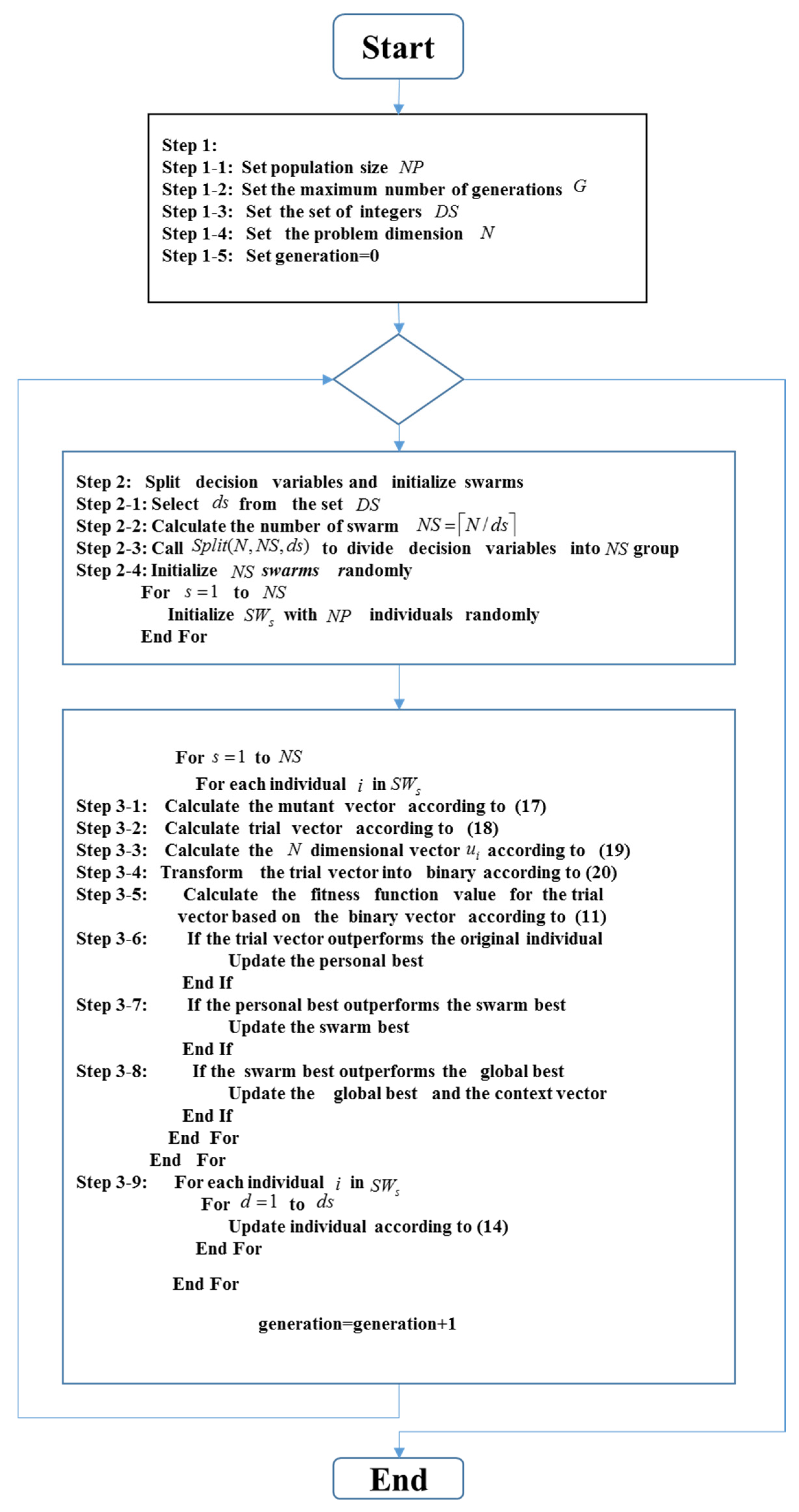
To describe the detailed operations of the Cooperative Coevolution (CC) approach, we define the notations used in

Table 3. Parameters, variables, and functions used in the algorithm.

Variable/Parameter	Meaning
$G$	total generations.
$t$	generation index.
$DS$	a set of integers for setting swarm dimensions.
$N$	$N={\displaystyle \sum _{d=1}^D{J}_d}+P$: problem dimension
$ds$	an integer selected from $DS.$
$NS$	$NS$= $⌈N/ds⌉$: the number of swarms, where $⌈N/ds⌉$ is the least integer greater than or equal to $N/ds.$
$s$	a swarm index, where $s\in \{1,2,\dots ,NS\}.$
$S{W}_s$	the $s$-th swarm.
$NP$	the population size in a swarm.
$\pi$	a permutation of the numbers in the set $\{1,2,\dots ,N\}.$
$R{G}_s$	the indices of decision variables associated with $S{W}_s,$ where $s\in \{1,2,\dots ,NS\}.$
$i$	the index of the $i$-th individual.
$S{W}_s.z_i$	the $i$-th individual in $S{W}_s.$
$S{W}_s.z_{id}$	the value of the $d$-th dimension of the $i$-th individual in $S{W}_s.$
$S{W}_s.\widehat{z}$	the best individual in $S{W}_s.$
$V_{\max }$	the maximum value of each dimension of an individual.
$\widehat{x}$	the $x$ component of the context vector obtained by concatenating the $x$ components of the best individual $S{W}_s.\widehat{z}$ for all $s\in \{1,2,\dots ,NS\}.$
$\widehat{y}$	the $y$ component of the context vector obtained by concatenating the $y$ component of the best individual $S{W}_s.\widehat{z}$ for all $s\in \{1,2,\dots ,NS\}.$
$\widehat{z}$	a context vector consisting of $x$ component and $y$ component.
$z_i$	a $N$ dimensional vector.
$S{W}_s.v_i$	a mutant vector for $S{W}_s.z_i$
$S{W}_s.v_{id}$	the value of the $d$-th dimension of $S{W}_s.v_i$
$S{W}_s.u_i$	a trial vector of $S{W}_s.v_i$
$S{W}_s.u_{id}$	the value of the $d$-th dimension of $S{W}_s.u_i$
$\mathrm{\Gamma }(i,s,S{W}_s.u_i,\widehat{z})$	a function that returns a $N$ dimensional vector defined in Function 1.
$u_i$	$u_i=\mathrm{\Gamma }(i,s,S{W}_s.u_i,\widehat{z}).$
$T(u_i)$	a function to transform $u_i$ to a binary vector defined in Function 2.
${\overline{u}}_i$	${\overline{u}}_i=T(u_i)$: a binary vector obtained by invoking $T(u_i).$
${\overline{z}}_s$	a $N$ dimensional binary vector representing the swarm best of $S{W}_s.$
$\overline{\widehat{z}}$	a $N$ dimensional binary vector of the global best.
${\rm N}(\mu ,{\sigma }^2)$	Gaussian distribution, where $\mu$ is the mean and ${\sigma }^2$ is the variance.
$sigmoid(z)$	$sigmoid(z)={\displaystyle \frac{1}{1+{\exp }^{-z}}}.$
$F_1(x,y)$	a fitness function,.
$f_i$	Scale factor for individual $i$ in a DE algorithm.
$Uniform(0,n)$	a random number in [0 $n$] generated by Uniform distribution.
$cr$	Crossover rate in a DE algorithm.
$Split(N,NS,ds)$	A function for splitting $N$ decision variables to $NS$ group randomly with each group consisting of at most $ds$ variables.

. Figure 1 shows the flowchart of the proposed CC–DE algorithm.

The function $Split(N,NS,ds)$ defined in Table 3 is used to randomly split the $N$ decision variables into the $NS$ group, each group with $ds$ variables. As the dimension of each group of decision variables is no greater than $ds$, the dimension of each individual is less than $N$.

The standard Differential Evolution approach improves an individual in a population by following three steps: creating a mutant vector, performing a crossover operation on the mutant vector to obtain a trial vector, constructing a dimensional vector to evaluate the performance of the trial vector, and selecting the trial vector if it outperforms the original individual. When the CC approach is combined with Differential Evolution, the algorithm improves an individual in a swarm by creating a mutant vector, performing a crossover operation on the mutant vector to obtain a trial vector, constructing a $N$ dimensional vector $u_i$, transforming $u_i$ into a binary vector ${\overline{u}}_i$ to evaluate the performance of the trial vector, and selecting the trial vector if it outperforms the original individual in the swarm. A mutant vector $S{W}_s.v_{id}$ in a swarm is computed according to (17). An element of the trial vector $S{W}_s.u_{id}$ in the $d$-th dimension is computed according to (18) based on the mutant vector $S{W}_s.v_{id}$. As the trial vector $S{W}_s.u_i$ considers only the decision variables in the swarm $S{W}_s$, we need to construct a $N$ dimensional vector based on $S{W}_s.u_i$ and the context vector $\widehat{z}$ according to (19) before evaluating the quality of the individual. The function $\mathrm{\Gamma }(i,s,S{W}_s.u_i,\widehat{z})$ defined in Function 1 is called in (19) to construct $N$ dimensional vector $u_i$ according to individual $S{W}_s.u_i$ and the context vector $\widehat{z}$. As the trial vector $u_i$ is real, we must transform it into a binary vector ${\overline{u}}_i$ by calling the function $T(u_i)$ defined in Function 2 according to (20) before computing the fitness function.

$$S{W}_s.v_{id}\leftarrow S{W}_s.z_{r_{1}d}+f_i(S{W}_s.z_{r_{2}d}-S{W}_s.z_{r_{3}d})$$

(17)

$$S{W}_s.u_{id}=\left\{\begin{array}{l}S{W}_s.v_{id} if Uniform(0,1)<c{r}_{DE}\\ S{W}_s.z_{id} otherwise\end{array}\right.$$

(18)

$$u_i=\mathrm{\Gamma }(i,s,S{W}_s.u_i,\widehat{z})$$

(19)

$${\overline{u}}_i=T(u_i)$$

(20)

Function 1  $\mathrm{\Gamma }(i,s,S{W}_s.u_i,\widehat{z})$

Input: $i,s,S{W}_s.u_i,\widehat{z}$

Output: $u_i$

For each $d\in \{1,2,\dots ,N\}$ If $d\in R{G}_s$                $u_{id}\leftarrow S{W}_s.u_{id}$ Else                $u_{id}\leftarrow {\widehat{z}}_d$ End If End For                Return $u_i$

Function 2  $T(u_i)$

Input: $u_i$

Output: ${\overline{u}}_i$

For each $d\in \{1,2,\dots ,N\}$              If $u_{id}>V_{\max }$                 $u_{id}\leftarrow V_{\max }$              Else If $u_{id}<-V_{\max }$                 $u_{id}\leftarrow -V_{\max }$              End If                Generate a random value $rsid$ from uniform distribution $Uniform(0,1)$                 ${\overline{u}}_{id}=\left\{\begin{array}{l}1 rsid<sigmoid(u_{id})\\ 0 otherwise\end{array}\right.$, where $sigmoid(u_{id})={\displaystyle \frac{1}{1+{\exp }^{-u_{id}}}}$ End For Return ${\overline{u}}_i$

4. Results

To verify the effectiveness of the new algorithm for solving the optimization problem for trust-based ridesharing systems, we conducted experiments and compared the results obtained by the CC–DE algorithm with those obtained by other competitive algorithms. The comparison with other competitive algorithms is based on four metrics: (1) performance metric, (2) robustness metric, (3) convergence rate metric, and (4) runtime metric. The performance metric is evaluated based on average fitness function values. The robustness metric is assessed based on the standard deviation of fitness function values. The convergence rate metric is based on average generations. The runtime metric is based on average runtime. We compare the 17 algorithms by analyzing the results for the four metrics as follows.

All the metaheuristic algorithms used for comparison with the proposed CC–DE algorithm were developed based on highly cited papers. The DE-1, DE-2, DE-3, DE-4, DE-5, and DE-6 algorithms were developed based on the highly cited paper [47]. The NSDE algorithm was developed based on the papers [48,49]. The PSO algorithm was developed based on the paper [50]. The SaNSDE algorithm was developed based on DE [47] and the concept of self-adaptation in paper [51]. The ALPSO algorithm was developed based on [52]. The Firefly algorithm was developed based on [53]. In summary, the algorithms used in this study are based on commonly used metaheuristic algorithms and their variants.

4.1. Experimental Setup

The algorithms to be compared include the proposed CC–DE algorithm, six standard DE algorithms, the NSDE algorithm, six two-head-based SaNSDE algorithms, the Firefly algorithm, the PSO algorithm, and a variant of the PSO algorithm called the ALPSO algorithm. The parameters of these algorithms used in the experiments are listed in

Table 4. Algorithmic specific parameters.

Algorithm	Parameters	Generation	Population Size	Maximum Value
DE-1	$c{r}_{DE}$ = 0.5 $f_i$: generated from $Uniform(0,2)$	$G$ = 10,000	$NP$ = 30	$V_{\max }$ = 4
DE-2	$c{r}_{DE}$ = 0.5 $f_i$: generated from $Uniform(0,2)$	$G$ = 10,000	$NP$ = 30	$V_{\max }$ = 4
DE-3	$c{r}_{DE}$ = 0.5 $f_i$: generated from $Uniform(0,2)$	$G$ = 10,000	$NP$ = 30	$V_{\max }$ = 4
DE-4	$c{r}_{DE}$ = 0.5 $f_i$: generated from $Uniform(0,2)$	$G$ = 10,000	$NP$ = 30	$V_{\max }$ = 4
DE-5	$c{r}_{DE}$ = 0.5 $F_i$: generated from $Uniform(0,2)$	$G$ = 10,000	$NP$ = 30	$V_{\max }$ = 4
DE-6	$c{r}_{DE}$ = 0.5 $f_i$: generated from $Uniform(0,2)$	$G$ = 10,000	$NP$ = 30	$V_{\max }$ = 4
SaNSDE(1,2)	$L$ = 1000, $cr$ = 0.5	$G$ = 10,000	$NP$ = 30	$V_{\max }$ = 4
SaNSDE(1,3)	$L$ = 1000, $cr$ = 0.5	$G$ = 10,000	$NP$ = 30	$V_{\max }$ = 4
SaNSDE(1,4)	$L$ = 1000, $cr$ = 0.5	$G$ = 10,000	$NP$ = 30	$V_{\max }$ = 4
SaNSDE(2,3)	$L$ = 1000, $cr$ = 0.5	$G$ = 10,000	$NP$ = 30	$V_{\max }$ = 4
SaNSDE(2,4)	$L$ = 1000, $cr$ = 0.5	$G$ = 10,000	$NP$ = 30	$V_{\max }$ = 4
SaNSDE(3,4)	$L$ = 1000, $cr$ = 0.5	$G$ = 10,000	$NP$ = 30	$V_{\max }$ = 4
PSO	$c_1$ = 0.4, $c_2$ = 0.6, $\omega$ = 0.4	$G$ = 10,000	$NP$ = 30	$V_{\max }$ = 4
ALPSO	$c_1$ = 0.4, $c_2$ = 0.6, $\omega$ = 0.4, $pc$ = 0.5	$G$ = 10,000	$NP$ = 30	$V_{\max }$ = 4
FA	${\beta }_0$ = 1.0, $\gamma$ = 0.2, $\gamma \alpha$ = 0.2	$G$ = 10,000	$NP$ = 30	$V_{\max }$ = 4
NSDE	$c{r}_{NSDE}$ = 0.5 $f_i$ = $0.5r_1+0.5$, where $r_1$ is generated from Gaussian distribution $N(0,1)$	$G$ = 10,000	$G$ = 10,000	$G$ = 10,000
CC–DE	$DS$ = {2, 5, 10, 15, 20, 25, 30, 35, 40, 45, 50, 55, 60, 65, 70}, $c{r}_{DE}$ = 0.5, $f_i$: generated from $Uniform(0,2)$	$G$ = 10,000	$G$ = 10,000	$G$ = 10,000

, where $G$, $NP$ and $V_{\max }$ are common parameters and other parameters are algorithm-specific parameters.

Ten test cases are used in the experiments. The data for the test cases can be downloaded from the link in [54].

Generation of test cases requires the function to generate drivers’ itineraries and the function to generate riders’ itineraries. The data generated for drivers are based on the specified number of drivers, the capacity of cars, the travel distance range of drivers, and the maximum number of bids. The data generated for riders are based on the specified number of riders, the number of seats requested, the travel distance range of riders, and the maximum detour ratio to transport riders. The maximum detour ratio is used to increase the probability of generating rider itineraries that can be matched. Fuel price is also considered in the generation of test cases to compute the bid price of riders and transport cost of drivers. The problem formulation is based on the assumption that the trust level data between drivers and riders and the trust requirements are available. It is assumed that the trust level data between drivers and riders has been extracted based on the historical ridesharing reputation records of drivers and riders, and the trust requirements have been set by drivers and riders. We set the trust level data and the trust requirements between drivers and riders according to the scenario to be simulated. For the existence of a solution, the trust level between drivers and riders on the same rides must be greater than or equal to the minimal trust level requested by drivers and riders. Readers may refer to the two scenarios provided in Section 5.1 of [27] and [35] for details about the generation of test case data.

4.2. Comparison Based on Performance Metric

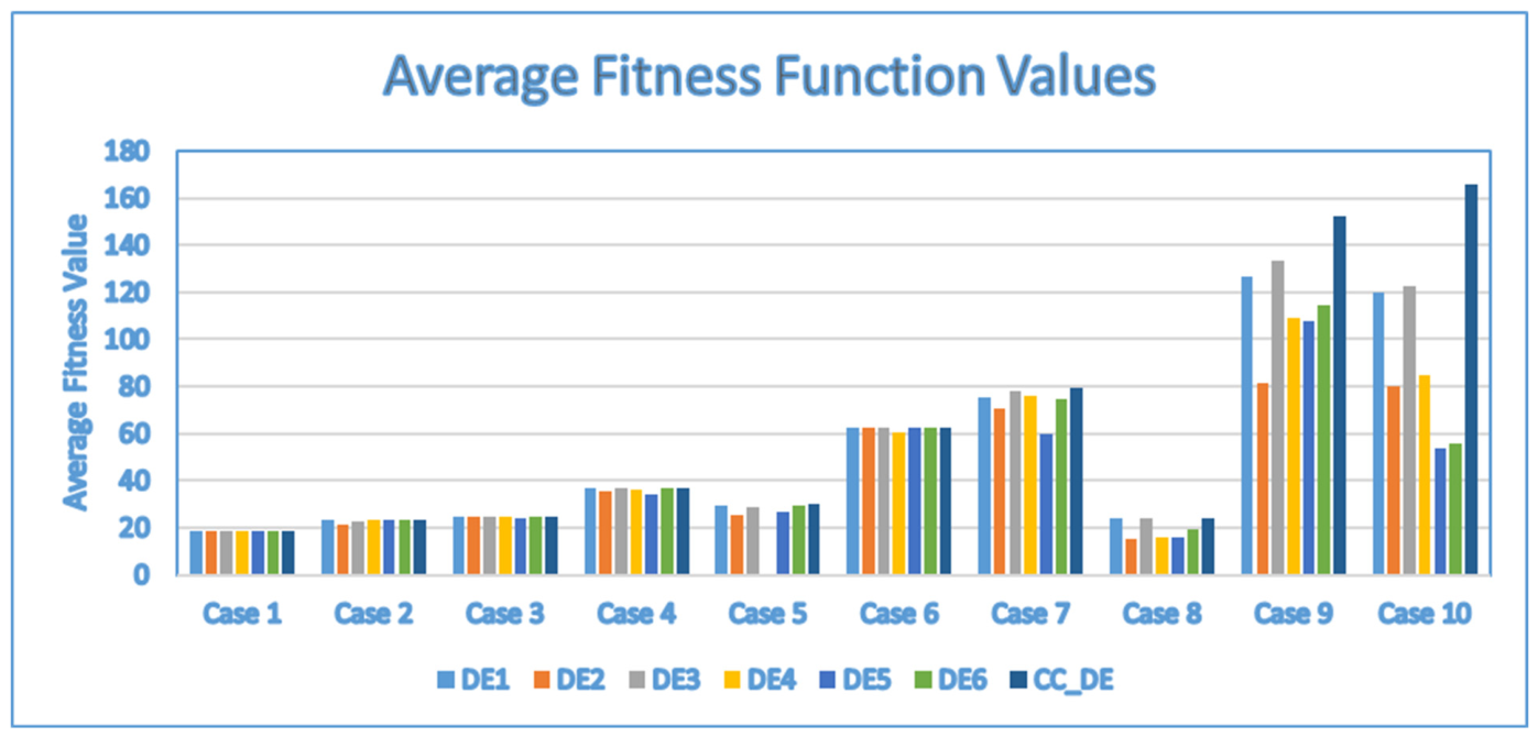
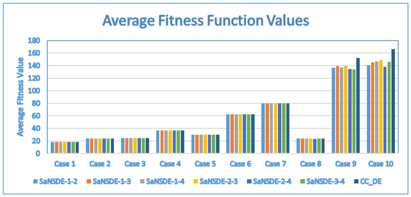
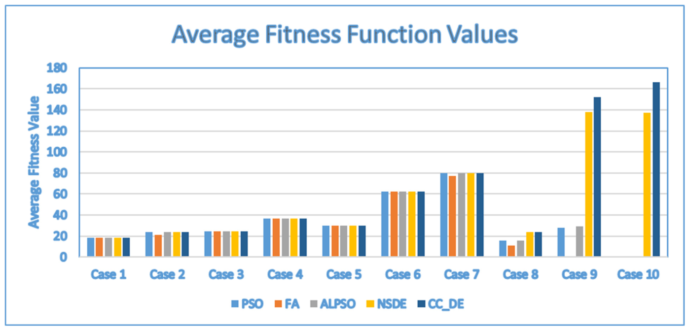
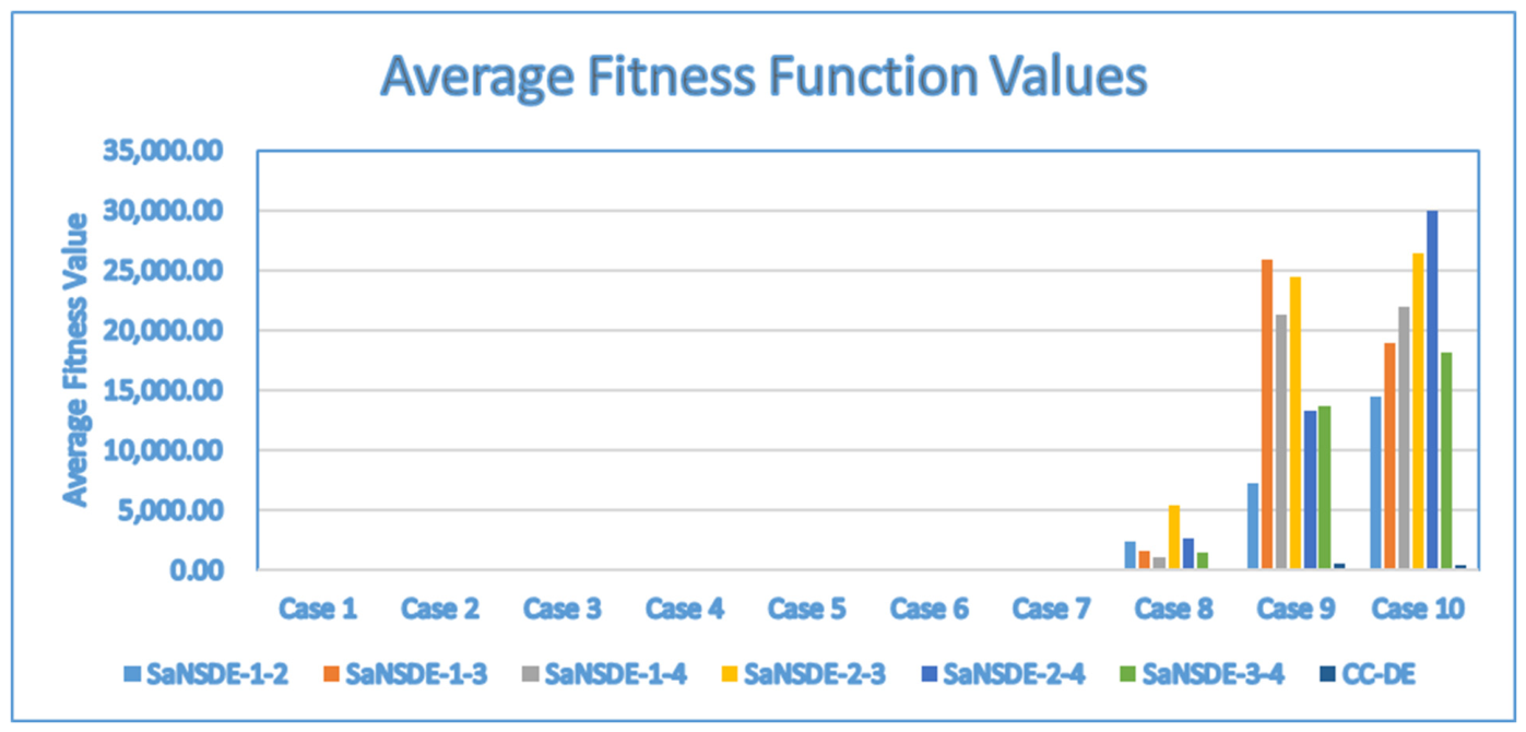
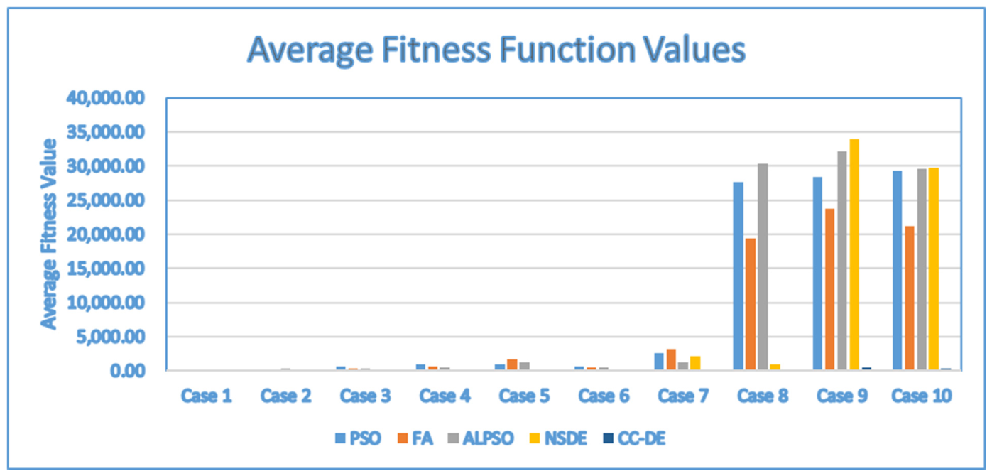
We evaluated the performance metric based on average fitness function values. The results are shown in

Table 5. Average fitness values for DE with six strategies and CC–DE algorithms.

Test Case	Participant (D/P)	DE1	DE2	DE3	DE4	DE5	DE6	CC–DE
1	4/10	18.305	18.305	18.305	18.305	18.305	18.305	18.305
2	5/11	23.518	21.1662	22.7885	23.518	23.518	23.518	23.518
3	5/12	24.79	24.79	24.3962	24.3962	24.0024	24.3962	24.79
4	6/12	36.58	35.4095	36.58	35.9755	34.1465	36.58	36.58
5	7/13	29.2442	25.482	29.0007	26.2379	26.8132	29.2442	30.063
6	8/14	62.18	62.18	62.18	60.7055	62.18	62.18	62.18
7	9/15	75.1808	70.481	78.1356	76.2821	59.7039	74.4286	79.64
8	20/20	23.644	15.4555	23.644	16.1718	16.0075	19.3717	23.644
9	30/30	126.2855	81.1175	133.3518	108.7805	107.5981	114.6592	151.977
10	40/40	120.0865	79.7772	122.8838	84.8821	53.8039	55.685	165.963

,

Table 6. Average fitness values for SaNSDE with the two combinations of strategies and CC–DE.

Test Case	Participant (D/P)	SaNSDE(1,2)	SaNSDE(1,3)	SaNSDE(1,4)	SaNSDE(2,3)	SaNSDE(2,4)	SaNSDE(3,4)	CC–DE
1	4/10	18.305	18.305	18.305	18.305	18.305	18.305	18.305
2	5/11	23.518	23.518	23.518	23.518	23.518	23.518	23.518
3	5/12	24.79	24.79	24.79	24.79	24.79	24.79	24.79
4	6/12	36.58	36.58	36.58	36.58	36.58	36.58	36.58
5	7/13	30.063	30.063	30.063	30.063	30.063	30.063	30.063
6	8/14	62.18	62.18	62.18	62.18	62.18	62.18	62.18
7	9/15	79.64	79.64	79.64	79.64	79.64	79.64	79.64
8	20/20	23.644	23.644	23.644	23.644	23.3851	23.644	23.644
9	30/30	136.5409	139.1137	137.1057	139.4738	134.7833	133.6144	151.977
10	40/40	140.6477	145.0836	146.8872	148.8646	137.7995	146.1111	165.963

and

Table 7. Average fitness values for PSO, FA, ALPSO, and CC-DE1.

Test Case	Participant (D/P)	PSO	FA	ALPSO	NSDE	CC–DE
1	3/10	18.305	18.305	18.305	18.305	18.305
2	5/11	23.518	20.9662	23.518	23.518	23.518
3	5/12	24.79	24.3962	24.79	24.79	24.79
4	6/12	36.58	36.58	36.58	36.58	36.58
5	7/13	30.063	30.063	30.063	30.063	30.063
6	8/14	62.18	62.18	62.18	62.18	62.18
7	9/15	79.64	77.3834	79.64	79.64	79.64
8	20/20	15.6939	10.8847	15.7567	23.5513	23.644
9	30/30	27.9224	−2.3761	28.9539	137.655	151.977
10	40/40	−2.5351	−4.0021	−0.5502	137.2235	165.963

for all the algorithms. Figure 2, Figure 3 and Figure 4 show the bar charts of the results of Table 5, Table 6 and Table 7, respectively.

Table 5 shows the average fitness values for the six DE algorithms corresponding to the six standard DE strategies and the CC–DE algorithm. The results show that the fitness function values obtained by the CC–DE algorithm are either the same as or greater than those obtained by the six DE algorithms. For smaller test cases such as Test Cases 1–7, the fitness function values obtained by the CC–DE algorithm are either the same as or close to those obtained by the six DE algorithms. The CC–DE algorithm significantly outperforms the six DE algorithms as the problem size grows.

Table 6 compares the average fitness values obtained by six SaNSDE variants and the proposed CC–DE algorithm. All algorithms achieve identical average fitness values on the first seven test cases, which indicates similar optimization performance on small-scale problems. On Test Case 8, CC–DE achieves the same highest average fitness value as five SaNSDE variants, while SaNSDE(2,4) produced a slightly lower value. More substantial differences occur on the two largest test cases. CC–DE obtains the highest average fitness values of 151.977 and 165.963 for Test Cases 9 and 10, respectively, and outperforms all six SaNSDE variants. These results suggest that the Cooperative Coevolution strategy employed by CC–DE becomes more effective as the problem size and search complexity increase.

Table 7 compares the performance of PSO, FA, ALPSO, NSDE, and the proposed CC–DE in terms of average fitness value. For the first seven test cases, CC–DE, NSDE, PSO, and ALPSO generally obtain identical average fitness values, whereas FA produces slightly inferior results on several instances. As the problem size increases, the superiority of CC–DE becomes evident. CC–DE achieves the highest average fitness values on Test Cases 8–10, outperforming all competing algorithms, with the largest improvement observed on the two largest problem instances. These results demonstrate that CC–DE provides superior solution quality and scalability and show it is highly effective for solving large and complex ridesharing optimization problems.

The Friedman test was conducted to statistically evaluate the differences among the 17 algorithms. The results of the Friedman test are as follows:

• Number of algorithms: 17
• Degrees of freedom: 16
• p-value: 1.12785 × 10⁻⁴ = 0.0001128

Therefore, the null hypothesis that all algorithms have equivalent performance is rejected. There is a statistically significant difference in the performance of the 17 algorithms. CC-DE1 achieved the lowest average rank (5.70), indicating the best overall ranking among the evaluated algorithms. In post-hoc comparisons, there are many pairwise p-values below 0.05. For example, for DE-5 and CC-DE1, the p-value is 0.00105. This indicates that there is a statistically significant difference between DE-5 and CC-DE1 at α = 0.05. For DE-2 and CC-DE1, the p-value is 0.00105. This indicates that there is a statistically significant difference between DE-2 and CC-DE1 at α = 0.05.

The Friedman test confirms significant differences among the compared algorithms. According to the average rankings in

Table 8. Average fitness rankings of the 17 algorithms from the Friedman test with $NP$ = 30.

Algorithm	Ranking
CC–DE	5.7
SaNSDE(2,3)	5.9
SaNSDE(1,3)	6.3
SaNSDE(1,4)	6.3
SaNSDE(1,2)	6.7
SaNSDE(3,4)	6.7
NSDE	7.15
SaNSDE(2,4)	7.45
DE-1	9
ALPSO	9.65
PSO	9.75
DE-3	10.2
DE-6	10.95
FA	12.35
DE-4	12.7
DE-2	13.1
DE-5	13.1

, CC–DE achieved the best ranking (5.70), followed by SaNSDE-2-3 (5.90) and SaNSDE-1-3/SaNSDE-1-4 (6.30).

4.3. Comparison Based on Robustness Metric

Table 9. Standard deviation of fitness function values obtained by six DE algorithms and the CC–DE algorithm.

Test Case	Participant (D/P)	DE1	DE2	DE3	DE4	DE5	DE6	CC–DE
1	4/10	0	0	0	0	0	0	0
2	5/11	0	5.3861	2.3068	0	0	0	0
3	5/12	0	0	1.2453	1.2453	1.6604	1.2453	0
4	6/12	0	2.4341	0	0.9733	4.3117	0	0
5	7/13	2.5892	4.9099	3.3592	7.1979	7.3465	2.5892	0
6	8/14	0	0	0	4.6667	0	0	0
7	9/15	6.4905	10.7481	3.1715	6.1819	18.2882	7.6642	0
8	20/20	0	9.1679	0	11.352	9.5636	8.6012	0
9	30/30	7.5179	42.649	6.4303	23.3827	17.3908	42.2574	0
10	40/40	24.6568	40.0971	14.6951	57.3518	52.6827	49.2159	0

presents the standard deviation of the fitness values obtained by six DE variants and the proposed CC–DE algorithm. A smaller standard deviation indicates better robustness and stability. The results show that CC–DE achieves a standard deviation of zero for all ten test cases. This demonstrates that it consistently obtains the same fitness values across independent runs. Although several DE variants also achieve zero standard deviation on small-scale problems, their stability deteriorates significantly as the problem size increases. In particular, for the largest test cases, several DE algorithms exhibit large variations in fitness values, while CC–DE maintains stability. These results indicate that the Cooperative Coevolution strategy effectively improves the robustness of CC–DE, enabling it to provide reliable and consistent optimization performance for large-scale optimization problems.

Table 10. Standard deviation of fitness function values obtained by six SaNSDE algorithms and the CC–DE algorithm.

Test Case	Participant (D/P)	SaNSDE(1,2)	SaNSDE(1,3)	SaNSDE(1,4)	SaNSDE(2,3)	SaNSDE(2,4)	SaNSDE(3,4)	CC–DE
1	4/10	0	0	0	0	0	0	0
2	5/11	0	0	0	0	0	0	0
3	5/12	0	0	0	0	0	0	0
4	6/12	0	0	0	0	0	0	0
5	7/13	0	0	0	0	0	0	0
6	8/14	0	0	0	0	0	0	0
7	9/15	0	0	0	0	0	0	0
8	20/20	0	0	0	0	0.5726	0	0
9	30/30	8.2936	5.282	5.3107	6.2373	17.8232	7.1908	0
10	40/40	17.4025	12.615	12.9272	10.1718	21.8929	14.6334	0

presents the standard deviations of the fitness values obtained by six SaNSDE variants and CC–DE. The smaller the standard deviation, the better the robustness and stability. For the first seven test cases, all algorithms achieve zero standard deviation, which indicates that they consistently obtained identical solutions for relatively small-scale problems. On Test Case 8, only SaNSDE(2,4) exhibits slight variability, while the other algorithms, including CC–DE, maintain zero standard deviation. However, for the two largest test cases, the robustness advantage of CC–DE becomes evident. CC–DE achieves zero standard deviation on both Test Cases 9 and 10, whereas all SaNSDE variants produce non-zero deviations. In particular, several SaNSDE variants exhibit large variations in fitness values and show reduced stability when solving large-scale optimization problems. These results indicate that the Cooperative Coevolution strategy significantly improves the robustness of CC–DE and makes it possible to consistently obtain high-quality solutions across independent runs.

Table 11. Standard deviation of fitness function values obtained by PSO, FA, ALPSO, NSDE, and CC–DE algorithms.

Test Case	Participant (D/P)	PSO	FA	ALPSO	NSDE	CC–DE
1	3/10	0	0	0	0	0
2	5/11	0	8.0695	0	0	0
3	5/12	0	1.2453	0	0	0
4	6/12	0	0	0	0	0
5	7/13	0	0	0	0	0
6	8/14	0	0	0	0	0
7	9/15	0	3.6634	0	0	0
8	20/20	7.005	5.9872	4.8561	0.2931	0
9	30/30	35.4394	0.3173	44.2064	8.9762	0
10	40/40	0.4426	0.4885	6.5933	18.3310	0

presents the standard deviations of the fitness values obtained by PSO, FA, ALPSO, NSDE, and CC–DE. A smaller standard deviation implies better robustness and stability. For the first seven test cases, CC–DE achieves zero standard deviation and indicates that it consistently obtains identical solutions across independent runs. Although most competing algorithms also exhibit stable behavior on small-scale problems, their robustness deteriorates as the problem size increases. For Test Cases 8–10, CC–DE maintains a standard deviation of zero, while PSO, FA, ALPSO, and NSDE exhibit varying degrees of instability. In particular, PSO, ALPSO, and NSDE show relatively large deviations on the largest test cases and reduced robustness for complex optimization problems. These results confirm that the Cooperative Coevolution strategy effectively enhances the robustness of CC–DE, enabling it to achieve reliable and consistent optimization performance.

Table 12. Average standard deviation rankings of the 17 algorithms from the Friedman test with $NP$ = 30.

Algorithm	Ranking
CC–DE	5.7
SaNSDE(1,3)	6.4
SaNSDE(2,3)	6.5
SaNSDE(1,4)	6.6
SaNSDE(3,4)	7.0
SaNSDE(1,2)	7.4
PSO	7.95
NSDE	8.05
ALPSO	8.25
SaNSDE(2,4)	8.45
DE-1	9.1
FA	9.15
DE-3	9.9
DE-6	11.85
DE-2	13.2
DE-5	13.6
DE-4	13.0

shows the average standard deviation rankings of the 17 algorithms. The Friedman test results with p-value: 0.0002368 demonstrate that the 17 algorithms have significantly different robustness levels in terms of the average standard deviation of solutions. CC–DE achieves the best average ranking and shows the highest stability among the compared algorithms. SaNSDE variants also show excellent robustness and obtain rankings close to CC–DE. In contrast, several conventional DE variants, especially DE-4, DE-5, and DE-2, exhibit larger variations and weaker robustness.

4.4. Comparison Based on Convergence Rate Metric

Table 13. Average number of generations for six DE algorithms and the CC–DE algorithm.

Test Case	Participant (D/P)	DE1	DE2	DE3	DE4	DE5	DE6	CC–DE
1	4/10	14.3	20.9	19.2	35.9	15.7	16	28.9
2	5/11	54.6	129.1	514.3	577.1	25.9	63.5	26.3
3	5/12	63.3	334.9	69.6	171.8	413.2	77.9	104.3
4	6/12	167.6	419.5	214.2	212.9	202	135.1	33.1
5	7/13	968.5	73.4	181	139.1	478.5	203.7	54.5
6	8/14	48.7	42.5	51.8	1056.4	341.2	41.7	26.9
7	9/15	860	165.5	932.7	1139.3	1054.7	1004	48.6
8	20/20	475	9261.1	1098.6	5027	14,904.6	6478.8	170.11
9	30/30	26,507.9	211.6	20,689.3	19,178	15,306.9	15,030	556.1
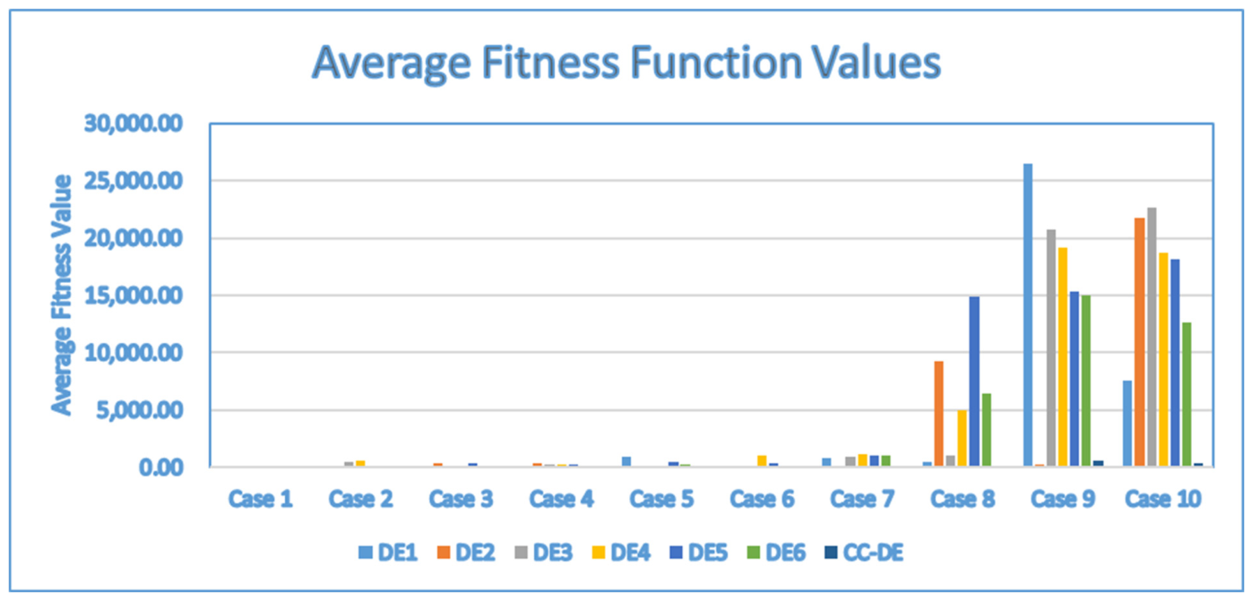
10	40/40	7556.1	21,756.2	22,660.2	18,684.8	18,172.4	12,640.3	392.8

compares the average number of generations required by six DE variants and the proposed CC–DE to obtain their best solutions. Figure 5 shows the bar charts of the results of Table 13. For the smaller test cases, several conventional DE variants converge as quickly as or slightly faster than CC–DE. However, as the problem size increases, the convergence advantage of CC–DE becomes increasingly evident. CC–DE achieves the fastest convergence on Test Cases 4–8 and 10, and ranks second on Test Case 9. In particular, for the largest problem instances, CC–DE required only 170.11, 556.1, and 392.8 generations on Test Cases 8–10, respectively, whereas most conventional DE variants require several thousand or even tens of thousands of generations. These results demonstrate that the Cooperative Coevolution strategy accelerates convergence on medium- and large-scale optimization problems while maintaining stable convergence behavior as the search space becomes increasingly complex.

Table 14. Average number of generations for six SaNSDE algorithms and the CC–DE algorithm.

Test Case	Participant (D/P)	SaNSDE(1,2)	SaNSDE(1,3)	SaNSDE(1,4)	SaNSDE(2,3)	SaNSDE(2,4)	SaNSDE(3,4)	CC–DE
1	4/10	2.6	2.3	3.4	2.7	1.9	2.7	28.9
2	5/11	7.2	10.6	5.6	6.1	5	5.3	26.3
3	5/12	8	8.7	6.3	8	7.7	8	104.3
4	6/12	9.3	21.1	8.2	7.8	10.4	12.2	33.1
5	7/13	12.1	19.6	10.3	9.8	7.6	11.2	54.5
6	8/14	7.2	8.6	7	7.5	6.5	8.8	26.9
7	9/15	145.5	95.7	47.6	25	172.9	79.9	48.6
8	20/20	2424.28	1628.5	1101.2	5433.6	2649.7	1428.4	170.11
9	30/30	7295.6	25,838	21,353.7	24,507.1	13,317.1	13,742.6	556.1
10	40/40	14,509.8	18,991.4	21,980.7	26,449.7	29,949.8	18,187.1	392.8

compares the average number of generations required by six SaNSDE variants and the proposed CC–DE to obtain their best solutions. Figure 6 shows the bar charts of the results of Table 14. For the first six test cases, the SaNSDE variants converge considerably faster than CC–DE and require only a few generations to reach the best solutions. However, as the problem size increased, the convergence advantage gradually shifted toward CC–DE. On Test Case 7, CC–DE ranks third among the seven algorithms. CC–DE achieves the fastest convergence on the three largest test cases, requiring only 170.1, 556.1, and 392.8 generations for Test Cases 8–10, respectively, whereas the SaNSDE variants require several thousand or even tens of thousands of generations. These results demonstrate that the Cooperative Coevolution strategy substantially improves convergence speed for large-scale optimization problems and exhibits much better scalability than the original SaNSDE variants.

Table 15. Average number of generations for PSO, FA, ALPSO, NSDE, and CC–DE.

Test Case	Participant (D/P)	PSO	FA	ALPSO	NSDE	CC–DE
1	3/10	43.6	52.7	82.5	106.9	28.9
2	5/11	233.1	134.9	266.6	51.2	26.3
3	5/12	691.8	328.3	406.9	49.8	104.3
4	6/12	929.1	573.1	548.6	154.54	33.1
5	7/13	969.5	1618.6	1196.6	118	54.5
6	8/14	638.3	546.5	483.4	36.9	26.9
7	9/15	2643.4	3206	1245.1	2173.4	48.6
8	20/20	27,714.3	19,374.3	30,399.2	911.6	170.11
9	30/30	28,346.9	23,731.4	32,209	33,899.3	556.1
10	40/40	29,242.7	21,267.9	29,617.2	29,677.1	392.8

compares the convergence speed of PSO, FA, ALPSO, NSDE, and the proposed CC–DE based on the average number of generations required to obtain the best solutions. Figure 7 shows the bar charts of the results of Table 15. CC–DE achieves the fastest convergence in eight out of ten test cases. Although NSDE converges faster than CC–DE on Test Case 3, CC–DE significantly outperforms all competing algorithms on larger problem instances. In particular, for Test Cases 8–10, CC–DE required only 170.11, 556.1, and 392.8 generations, respectively, whereas the other algorithms require thousands or tens of thousands of generations. These results demonstrate that the Cooperative Coevolution strategy significantly improves convergence speed and scalability, which enables CC–DE to efficiently solve large-scale optimization problems.

The Friedman test results in

Table 16. Average generation rankings of the 17 algorithms from the Friedman test with $NP$ = 30.

Algorithm	Ranking
SaNSDE(1,2)	4.4
SaNSDE(1,4)	4.5
SaNSDE(3,4)	4.65
SaNSDE(2,4)	4.8
SaNSDE(2,3)	5.65
CC–DE	5.9
SaNSDE(1,3)	6.4
DE-1	8.7
DE-6	9.1
DE-2	10.0
DE-3	10.6
DE-5	10.6
NSDE	11
DE-4	11.9
FA	14.1
ALPSO	15.3
PSO	15.4

with p-value = 0.0000000000812 demonstrate that the 17 algorithms have significantly different convergence speeds. Among them, SaNSDE variants achieve the fastest convergence, obtaining the best average rankings. CC–DE provides highly competitive convergence performance, ranking sixth overall and outperforming most traditional algorithms. PSO, ALPSO, and FA exhibit slower convergence, requiring significantly more generations to find solutions.

4.5. Comparison Based on Runtime

Table 17. Average runtime for six DE algorithms and the CC–DE algorithm.

Test Case	Participant (D/P)	SaNSDE(1,2)	SaNSDE(1,3)	SaNSDE(1,4)	SaNSDE(2,3)	SaNSDE(2,4)	SaNSDE(3,4)	CC–DE
1	4/10	3.910036	3.438385	4.8654	3.851685	2.932878	3.778974	41.3244
2	5/11	150.0398	242.2169	122.0469	123.0377	98.0361	104.7114	52.73571
3	5/12	163.5201	183.8365	132.2039	174.3178	168.0882	175.2911	215.4942
4	6/12	218.6795	526.8189	211.0596	189.4576	247.1613	287.6342	76.65993
5	7/13	316.3241	582.3299	346.0051	317.1698	311.7581	306.3035	125.2045
6	8/14	164.0884	166.1341	136.0377	153.6055	133.2419	183.4569	61.51896
7	9/15	6660.315	4251.427	2056.433	989.167	6659.944	3060.694	181.8257
8	20/20	7900.67	5785.963	3864.998	19,252.28	8723.311	4665.84	223.3187
9	30/30	56,986.22	208,773.6	174,060.8	199,049.1	102,073.5	236,556.5	2930.783
10	40/40	29,1305	188,441.2	451,674	545,441.8	615,479.5	375,085.8	10,358.63

shows the average runtime for six DE algorithms and the CC–DE algorithm. The results indicate that the CC–DE algorithm outperforms the six DE algorithms with only a few exceptions in most test cases.

The results in

Table 18. Average runtime for six SaNSDE algorithms and the CC–DE algorithm.

Test Case	Participant (D/P)	DE1	DE2	DE3	DE4	DE5	DE6	CC–DE
1	4/10	9.97153	14.3853	13.5302	25.3827	10.8917	11.3347	41.3244
2	5/11	56.8719	145.926	573.841	577.44	25.0911	63.2511	52.73571
3	5/12	58.1069	316.089	66.0615	171.553	496.022	78.8854	215.4942
4	6/12	178.797	465.255	239.853	292.352	272.876	154.789	76.65993
5	7/13	1101.32	72.4208	203.697	142.095	522.498	222.73	125.2045
6	8/14	49.3448	51.0357	52.6708	1100.65	356.008	43.9827	61.51896
7	9/15	1457.18	246.911	1392.54	1617.9	1951.71	1821.89	181.8257
8	20/20	1518.28	31,984.9	3405	16,759	49,599	21,077.2	223.3187
9	30/30	187,195	1622.6	151,948	145,334	115,101	115,868	2930.783
10	40/40	153,532	448,303	457,858	383,688	377,135	260,440	10,358.63

show that the CC–DE algorithm outperforms the six SaNSDE algorithms in terms of runtime, with only a few exceptions in most test cases. Similarly, the CC–DE algorithm outperforms the PSO, FA, ALPSO, NSDE, and CC–DE algorithms in terms of runtime, with only a few exceptions in most test cases, according to the results in

Table 19. Average runtime for PSO, FA, ALPSO, NSDE, and CC–DE.

Test Case	Participant (D/P)	PSO	FA	ALPSO	NSDE	CC–DE
1	3/10	30.6979	44.209	2149.36	87.4453	41.3244
2	5/11	214	162.353	10,635	64.3712	52.73571
3	5/12	579.618	743.041	16,923.2	55.2481	215.4942
4	6/12	938.28	2068.15	24,987	210.323	76.65993
5	7/13	804.055	7978.87	58,197.6	172.069	125.2045
6	8/14	519.053	1213.66	20,345.1	45.7169	61.51896
7	9/15	2628.78	24,682.7	84,547.8	4002.97	181.8257
8	20/20	74,249.8	263,365	114,127	3312.9	223.3187
9	30/30	62,172.4	935,684	241,582	272,972	2930.783
10	40/40	284,972	2,247,490	524,182	606,176	10,358.63

.

The Friedman test detected significant differences among the runtimes of the 17 algorithms (p = 7.23 × 10⁻⁸). Therefore, the null hypothesis of equal performance was rejected.

Table 20. Average runtime rankings of the 17 algorithms from the Friedman test with $NP$ = 30.

Algorithm	Ranking
CC–DE	4.2
DE-1	5.3
DE-6	5.6
DE-3	7.5
DE-2	7.8
SaNSDE(1,4)	7.9
NSDE	7.9
SaNSDE(1,2)	8.0
SaNSDE(2,4)	8.2
SaNSDE(2,3)	8.5
SaNSDE(3,4)	8.8
DE-5	9.4
DE-4	9.9
SaNSDE(1,3)	10.1
PSO	11.8
FA	15.8
ALPSO	16.3

shows the average runtime rankings of the 17 algorithms from the Friedman test.

4.6. Contribution of Cooperative Coevolution to Performance and Sensitivity

We conducted experiments to investigate the contribution of Cooperative Coevolution to improving performance. To investigate this contribution, we disabled Cooperative Coevolution by setting the set $DS$ to contain only one integer that is greater than the total number of decision variables. In this way, there is only one group in the solution-finding process, and we can assess the performance after disabling Cooperative Coevolution. The results obtained by disabling Cooperative Coevolution are shown in the third column, whereas those obtained by enabling Cooperative Coevolution are shown in the fifth column of

Table 21. Comparison of Average fitness values for CC–DE algorithm with CC Disabled and CC Enabled.

Test Case	Participant (D/P)	CC–DE (Setting of $\mathit{D}\mathit{S}$ to Disable CCC)		CC–DE (Setting of $\mathit{D}\mathit{S}$ the Same as the One Used in the Experiments to Enable CC)
1	4/10	18.305	$DS$ = {20}	18.305
2	5/11	23.518	$DS$ = {20}	23.518
3	5/12	24.79	$DS$ = {20	24.79
4	6/12	36.58	$DS$ = {20}	36.58
5	7/13	25.969	$DS$ = {20}	30.063
6	8/14	60.7055	$DS$ = {25}	62.18
7	9/15	73.581	$DS$ = {30}	79.64
8	20/20	−1.4775	$DS$ = {100}	23.644
9	30/30	−2.6244	$DS$ = {100}	151.977
10	40/40	−4.7486	$DS$ = {100}	165.963

. It is obvious that the contribution of Cooperative Coevolution to the improvement of performance tends to increase as the problem dimension grows.

We conducted experiments to compare the performance of the CC–DE algorithm for different population sizes. The results in

Table 22. Average fitness values for the CC–DE algorithm with different population sizes.

Test Case	Participant (D/P)	CC–DE ($\mathit{N}\mathit{P}$ = 10)	CC–DE ($\mathit{N}\mathit{P}$ = 30)	CC–DE ($\mathit{N}\mathit{P}$ = 50)
1	4/10	18.305	18.305	18.305
2	5/11	23.518	23.518	23.518
3	5/12	24.79	24.79	24.79
4	6/12	36.58	36.58	36.58
5	7/13	36.58	30.063	30.063
6	8/14	62.18	62.18	62.18
7	9/15	79.64	79.64	79.64
8	20/20	23.644	23.644	23.644
9	30/30	151.977	151.977	151.977
10	40/40	165.963	165.963	165.963

show that the performance of the CC–DE algorithm remains the same for population sizes $NP$ = 10, $NP$ = 30, and $NP$ = 50. Therefore, the CC–sDE algorithm is insensitive to population size.

As the scaling factor is randomly generated in the CC–DE algorithm, the CC–DE algorithm does not rely on a fixed scaling factor value. The average number of generations for the CC–DE algorithm is much smaller than the generation parameter $G$ ($G$ = 10,000 for Case 1 through 7 and $G$ = 50,000 for Case 8 through 10). Therefore, the performance of the CC–DE algorithm is insensitive to the generation parameter $G$.

We have two observations as follows:

(i).

The results in Section 4.3 (Comparison Based on the Robustness Metric) show that the CC–DE algorithm achieves a standard deviation of zero for all ten test cases. This means that the CC–DE algorithm consistently finds the same best solution for each test case.

(ii).

The results in Section 4.2 (Comparison Based on the Performance Metric) show that the CC–DE algorithm generates the highest-quality solutions for all test cases when compared with the other 16 algorithms.

It follows from observations (i) and (ii) that the CC–DE algorithm consistently finds high-quality solutions for all test cases compared with the other 16 algorithms.

When evaluating the convergence speed of metaheuristic algorithms, researchers primarily use two metrics: average number of generations and average runtime. Average number of generations is a hardware-independent measure, whereas average runtime is highly dependent on hardware and implementation of algorithms. According to the experimental results, CC–DE ranks sixth in terms of average generations and first in terms of average runtime among the 17 algorithms. As all experiments were conducted on the same hardware, this indicates that software implementation is an important factor in improving the average runtime. Although CC–DE ranks first in terms of average fitness value and average runtime, it ranks sixth in terms of average generation due to the use of the complex Cooperative Coevolution mechanism.

5. Conclusions

Although social ridesharing and trust-based ridesharing have attracted the research community’s attention, they pose challenges in the development of an effective algorithm to solve the corresponding optimization problems. The core challenges in developing algorithms for social or trust-based ridesharing involve high computational complexity, matching constraints, and trust level requirements. The computational complexity challenge arises from non-convex and non-linear integer programming problems in social or trust-based ridesharing systems, and this makes exact optimization methods not applicable. Consideration of spatial, temporal, and social relationships between participating ridesharing partners in social or trust-based ridesharing systems increases the search space exponentially, leading to combinatorial explosion. Metaheuristic approaches excel at solving social and trust-based ridesharing problems because they can handle complex constraints, integrate non-linear social metrics, and often find high-quality solutions in practice. However, their effectiveness may vary depending on the type of metaheuristic approach used. The goal of this paper is to study the effectiveness of combining the Cooperative Coevolution approach with Differential Evolution (DE) to improve the performance of trust-based ridesharing systems. We proposed a CC–DE algorithm by combining the CC approach with DE. To verify the effectiveness of the new algorithm for solving the optimization problem for trust-based ridesharing systems, we conducted experiments and compared the results obtained by the new algorithm with those obtained by other competitive algorithms. The comparison with other competitive algorithms is based on three metrics: (1) performance metric, (2) robustness metric, and (3) convergence rate metric. The performance metric is evaluated based on average fitness function values. The robustness metric is assessed based on the standard deviation of fitness function values. The convergence rate metric is assessed based on the average number of generations required to find the best solution.

For smaller test cases such as Test Cases 1–7, the fitness function values obtained by the CC–DE algorithm are close to those obtained by the six DE algorithms. The CC–DE algorithm significantly outperforms the six DE algorithms as the problem size grows. The Friedman test was conducted to statistically evaluate the differences among the 17 algorithms. The Friedman test confirms significant differences among the compared algorithms. According to the average rankings, CC–DE achieves the best ranking (5.70), followed by SaNSDE-2-3 (5.90) and SaNSDE-1-3/SaNSDE-1-4 (6.30).

The Friedman test demonstrates that the 17 algorithms have significantly different robustness levels in terms of the average standard deviation of solutions. CC–DE achieves the best average ranking, indicating the highest stability among the compared algorithms. SaNSDE variants also show excellent robustness, obtaining rankings close to CC–DE. In contrast, several conventional DE variants, especially DE-4, DE-5, and DE-2, exhibit larger variations and weaker robustness. The Friedman test demonstrates that the 17 algorithms have significantly different convergence speeds. SaNSDE variants achieve the fastest convergence, obtaining the best average rankings. CC–DE provides highly competitive convergence performance, ranks sixth overall, and outperforms most traditional algorithms. PSO, ALPSO, and FA exhibit slower convergence, requiring significantly more generations to find solutions. In summary, comparison with other 16 competitive algorithms based on the experimental results shows that the proposed algorithm significantly outperforms other competitive algorithms in performance and robustness metrics. However, CC–DE exhibits slower convergence due to the divide-and-conquer by random grouping approach.

Despite the interesting findings presented in this paper, several limitations remain. The preliminary results were based on ten instances generated based on a specific area. Validation of the proposed method on a real operational ridesharing platform is an interesting issue. The method proposed in this study is based on static ridesharing conditions. Modification of the proposed method is required to address the dynamic ridesharing problems. The results of this study show that the CC approach can be combined with a standard DE to improve performance and robustness. A new finding of this study is that the proposed algorithm developed by combining a single DE strategy with the CC approach outperforms the six variants of SaNSDE algorithms in terms of performance and robustness, where each SaNSDE algorithm is developed by combining two DE strategies with a self-adaptation mechanism. An interesting future research direction is to study whether the CC approach can be combined with other evolutionary computation approaches to improve performance and robustness.

References

1. Agatz, N.; Erera, A.; Savelsbergh, M.; Wang, X. Optimization for dynamic ride-sharing: A review. Eur. J. Oper. Res. 2012, 223, 295–303. [Google Scholar] [CrossRef] [Scilit]
2. Furuhata, M.; Dessouky, M.; Ordóñez, F.; Brunet, M.; Wang, X.; Koenig, S. Ridesharing: The state-of-the-art and future direc-tions. Transp. Res. Part B Methodol. 2013, 57, 28–46. [Google Scholar] [CrossRef] [Scilit]
3. Ting, K.H.; Lee, L.S.; Pickl, S.; Seow, H.-V. Shared Mobility Problems: A Systematic Review on Types, Variants, Characteristics, and Solution Approaches. Appl. Sci. 2021, 11, 7996. [Google Scholar] [CrossRef] [Scilit]
4. Mourad, A.; Puchinger, J.; Chu, C. A survey of models and algorithms for optimizing shared mobility. Transp. Res. Part B Methodol. 2019, 123, 323–346. [Google Scholar] [CrossRef] [Scilit]
5. Martins, L.C.; Torre, R.; Corlu, C.G.; Juan, A.A.; Masmoudi, M.A. Optimizing ride-sharing operations in smart sustainable cities: Challenges and the need for agile algorithms. Comput. Ind. Eng. 2021, 153, 107080. [Google Scholar] [CrossRef] [Scilit]
6. Qin, Z.T.; Zhu, H.; Ye, J. Reinforcement learning for ridesharing: An extended survey. Transp. Res. Part C Emerg. Technol. 2022, 144, 103852. [Google Scholar] [CrossRef] [Scilit]
7. Tian, S.; He, Z.; Dai, R.; Wang, J.; Yang, H. Commute with Community: Enhancing Shared Travel through Social Networks. In Proceedings of the 2024 International Conference on Generative Artificial Intelligence and Information Security, Kuala Lumpur, Malaysia, 10–12 May 2024; ACM: New York, NY, USA, 2024; pp. 274–279. [Google Scholar]
8. Hsieh, F.-S. Assessment and Realization of the Benefits of Collaboration Among Ridesharing Service Providers Based on Metaheuristic Algorithms. Smart Cities 2026, 9, 42. [Google Scholar] [CrossRef] [Scilit]
9. Sarriera, J.M.; Álvarez, G.E.; Blynn, K.; Alesbury, A.; Scully, T.; Zhao, J. To share or not to share: Investigating the social aspects of dynamic ridesharing. Transp. Res. Rec. 2017, 2605, 109–117. [Google Scholar]
10. Prieto, M.; Stan, V.; Baltas, G. New insights in peer-to-peer carsharing and ridesharing participation intentions: Evidence from the “provider-user” perspective. J. Retail. Consum. Serv. 2022, 64, 102795. [Google Scholar] [CrossRef] [Scilit]
11. Mitropoulos, L.; Kortsari, A.; Ayfantopoulou, G. A systematic literature review of ride-sharing platforms, user factors and barriers. Eur. Transp. Res. Rev. 2021, 13, 61. [Google Scholar] [CrossRef] [Scilit] [PubMed]
12. Wang, K.; Qi, L.; Yang, S.; Wang, C.; Zhou, R.; Liu, J. Towards Sustainable Mobility: Factors Influencing the Intention to Use Ride-Sharing in the Post-Pandemic Era. Sustainability 2025, 17, 8343. [Google Scholar] [CrossRef] [Scilit]
13. Gangadharaiah, R.; Brooks, J.; Boor, L.; Kolodge, K.; Jia, Y. Barriers and Benefits: Understanding Riders’ Views on Pooled Rideshare in the US. Vehicles 2025, 7, 13. [Google Scholar] [CrossRef] [Scilit]
14. Si, H.; Shi, J.; Hua, W.; Cheng, L.; De Vos, J.; Li, W. What influences people to choose ridesharing? An overview of the literature. Transp. Rev. 2023, 43, 1211–1236. [Google Scholar] [CrossRef] [Scilit]
15. Su, H.; Gangadharaiah, R.; Rosopa, E.B.; Brooks, J.O.; Boor, L.; Kolodge, K.; Rosopa, P.J.; Jia, Y. Exploration of factors that influence willingness to consider pooled rideshare. Transp. Res. Rec. 2024, 2678, 57–73. [Google Scholar] [CrossRef] [Scilit]
16. Tang, L.; Duan, Z.; Zhao, Y. Toward using social media to support ridesharing services: Challenges and opportunities. Transp. Plan. Technol. 2019, 42, 355–379. [Google Scholar] [CrossRef] [Scilit]
17. Cici, B.; Markopoulou, A.; Frias-Martinez, E.; Laoutaris, N. Assessing the potential of ride-sharing using mobile and social data: A tale of four cities. In Proceedings of the 2014 ACM International Joint Conference on Pervasive and Ubiquitous Computing, Seattle, WA, USA, 13–17 September 2014; ACM: New York, NY, USA, 2014; pp. 201–211. [Google Scholar]
18. Vaclavik, M.C.; Macke, J.; Silva, D.F. ‘Do not talk to strangers’: A study on trust in Brazilian ridesharing apps. Technol. Soc. 2020, 63, 101379. [Google Scholar] [CrossRef] [Scilit]
19. Najjar, M.S.; Dahabiyeh, L. Trust in the ride hailing service of the sharing economy: The roles of legitimacy and process transparency. J. Organ. End User Comput. (JOEUC) 2021, 33, 1–24. [Google Scholar]
20. Cheng, X.; Su, L.; Yang, B. An investigation into sharing economy enabled ridesharing drivers’ trust: A qualitative study. Electron. Commer. Res. Appl. 2020, 40, 100956. [Google Scholar] [CrossRef] [Scilit]
21. Shao, Z.; Yin, H. Building customers’ trust in the ridesharing platform with institutional mechanisms: An empirical study in China. Internet Res. 2019, 29, 1040–1063. [Google Scholar]
22. Wu, M.; Neill, S. Trust transfer and the intention to use app-enabled carpooling service. Asia Pac. J. Mark. Logist. 2021, 33, 1498–1512. [Google Scholar] [CrossRef] [Scilit]
23. Xia, J.; Curtin, K.M.; Huang, J.; Wu, D.; Xiu, W.; Huang, Z. A carpool matching model with both social and route networks. Comp. Environ. Urban Syst. 2017, 75, 90–102. [Google Scholar]
24. Li, Y.; Chen, R.; Chen, L.; Xu, J. Towards Social-Aware Ridesharing Group Query Services. IEEE Trans. Serv. Comp. 2017, 10, 646–659. [Google Scholar] [CrossRef] [Scilit]
25. Li, Y.; Wan, J.; Chen, R.; Xu, J.; Fu, X.; Gu, H.; Lv, P.; Xu, M. Top-kk Vehicle Matching in Social Ridesharing: A Price-Aware Approach. IEEE Trans. Knowl. Data Eng. 2021, 33, 1251–1263. [Google Scholar]
26. Bistaffa, F.; Farinelli, A.; Chalkiadakis, G.; Ramchurn, S.D. A cooperative game-theoretic approach to the social ridesharing problem. Artif. Intell. 2017, 246, 86–117. [Google Scholar] [CrossRef] [Scilit]
27. Hsieh, F.-S. Trust-Based Recommendation for Shared Mobility Systems Based on a Discrete Self-Adaptive Neighborhood Search Differential Evolution Algorithm. Electronics 2022, 11, 776. [Google Scholar] [CrossRef] [Scilit]
28. Hsieh, F.S. Applying “Two Heads Are Better Than One” Human Intelligence to Develop Self-Adaptive Algorithms for Ridesharing Recommendation Systems. Electronics 2024, 13, 2241. [Google Scholar] [CrossRef] [Scilit]
29. Nabila, S.; Hashem, T.; Anwar, S.; Islam, A.A.A. Efficient algorithms for community aware ridesharing. GeoInformatica 2024, 28, 403–432. [Google Scholar] [CrossRef] [Scilit]
30. Shim, C.; Sim, G.; Chung, Y.D. Cohesive Ridesharing Group Queries in Geo-Social Networks. IEEE Access 2020, 8, 97418–97436. [Google Scholar] [CrossRef] [Scilit]
31. Shami, T.M.; El-Saleh, A.A.; Alswaitti, M.; Al-Tashi, Q.; Summakieh, M.A.; Mirjalili, S. Particle swarm optimization: A comprehensive survey. IEEE Access 2022, 10, 10031–10061. [Google Scholar] [CrossRef] [Scilit]
32. Pant, M.; Zaheer, H.; Garcia-Hernandez, L.; Abraham, A. Differential Evolution: A review of more than two decades of research. Eng. Appl. Artif. Intell. 2020, 90, 103479. [Google Scholar] [CrossRef] [Scilit]
33. Ahmad, M.F.; Isa, N.A.M.; Lim, W.H.; Ang, K.M. Differential evolution: A recent review based on state-of-the-art works. Alex. Eng. J. 2022, 61, 3831–3872. [Google Scholar] [CrossRef] [Scilit]
34. Van den Bergh, F.; Engelbrecht, A.P. A cooperative approach to particle swarm optimization. IEEE Trans. Evol. Comput. 2004, 8, 225–239. [Google Scholar] [CrossRef] [Scilit]
35. Hsieh, F.-S.; Zhan, F.-M.; Guo, Y.-H. A solution methodology for carpooling systems based on double auctions and cooperative coevolutionary particle swarms. Appl. Intell. 2018, 49, 741–763. [Google Scholar] [CrossRef] [Scilit]
36. Hsieh, F.-S. Improving Performance and Robustness of Particle Swarm Optimization Metaheuristic Algorithms for Ridesharing Systems Based on a Cooperative Coevolution Approach. Electronics 2026, 15, 1682. [Google Scholar] [CrossRef] [Scilit]
37. Shi, Y.J.; Teng, H.F.; Li, Z.Q. Cooperative co-evolutionary differential evolution for function optimization. In Advances in Natural Computation, Proceedings of the First International Conference, Changsha, China, 27–29 August 2005; Springer: Berlin/Heidelberg, Germany, 2005; pp. 1080–1088. [Google Scholar]
38. Trunfio, G.A. A cooperative coevolutionary differential evolution algorithm with adaptive subcomponents. Procedia Comput. Sci. 2015, 51, 834–844. [Google Scholar] [CrossRef] [Scilit][Green Version]
39. Hsieh, F.-S. One Plus One Is Greater than Two for Multiple Ridesharing Service Providers: A Theoretical Proof and an Algorithm for Sustainable Collaborative Ridesharing. Systems 2026, 14, 1012. [Google Scholar] [CrossRef] [Scilit]
40. Ma, X.; Li, X.; Zhang, Q.; Tang, K.; Liang, Z.; Xie, W.; Zhu, Z. A survey on cooperative co-evolutionary algorithms. IEEE Trans. Evol. Comput. 2018, 23, 421–441. [Google Scholar] [CrossRef] [Scilit]
41. Liu, Y.; Yao, X.; Zhao, Q.; Higuchi, T. Scaling up fast evolutionary programming with cooperative coevolution. In Proceedings of the 2001 Congress on Evolutionary Computation, Seoul, Republic of Korea, 27–30 May 2001; IEEE: New York, NY, USA, 2001; Volume 2, pp. 1101–1108. [Google Scholar]
42. Wu, Y.; Wang, L.; Zhuang, X.; Wang, J.J.; Chen, J.F.; Zheng, J. A cooperative coevolutionary algorithm with problem-specific knowledge for energy-efficient scheduling in seru system. Knowl.-Based Syst. 2023, 274, 110663. [Google Scholar] [CrossRef] [Scilit]
43. Yang, Z.; Tang, K.; Yao, X. Large scale evolutionary optimization using cooperative coevolution. Inf. Sci. 2008, 178, 2985–2999. [Google Scholar] [CrossRef] [Scilit]
44. Coello, C.A.C. Theoretical and numerical constraint-handling techniques used with evolutionary algorithms: A survey of the state of the art. Comput. Methods Appl. Mech. Eng. 2002, 191, 1245–1287. [Google Scholar] [CrossRef] [Scilit]
45. Deb, K. An efficient constraint handling method for genetic algorithms. Comput. Methods Appl. Mech. Eng. 2000, 186, 311–338. [Google Scholar] [CrossRef] [Scilit]
46. Hsieh, F.-S. Improving Performance and Robustness with Two Strategies in Self-Adaptive Differential Evolution Algorithms for Planning Sustainable Multi-Agent Cyber–Physical Production Systems. Appl. Sci. 2025, 15, 10266. [Google Scholar] [CrossRef] [Scilit]
47. Price, K.; Storn, R.; Lampinen, J. Differential Evolution: A Practical Approach to Global Optimization; Springer: Berlin/Heidelberg, Germany, 2005. [Google Scholar]
48. Das, S.; Abraham, A.; Chakraborty, U.K.; Konar, A. Differential evolution using a neighborhood-based mutation operator. IEEE Trans. Evol. Comput. 2009, 13, 526–553. [Google Scholar] [CrossRef] [Scilit]
49. Yang, Z.; He, J.; Yao, X. Making a difference to differential evolution. In Advances in Metaheuristics for Hard Optimization; Michalewicz, Z., Siarry, P., Eds.; Springer: Berlin/Heidelberg, Germany, 2007; pp. 415–432. [Google Scholar]
50. Kennedy, J.; Eberhart, R.C. Particle swarm optimization. In Proceedings of IEEE International Conference on Neural Networks, Perth, Australia, 27 November–1 December 1995; IEEE: New York, NY, USA, 1995; pp. 1942–1948. [Google Scholar]
51. Qin, A.K.; Suganthan, P.N. Self-adaptive differential evolution algorithm for numerical optimization. In Proceedings of the 2005 IEEE Congress on Evolutionary Computation, Edinburgh, UK, 2–5 September 2005; IEEE: New York, NY, USA, 2005; Volume 2, pp. 1785–1791. [Google Scholar]
52. Wang, F.; Zhang, H.; Li, K.; Lin, Z.; Yang, J.; Shen, X.L. A hybrid particle swarm optimization algorithm using adaptive learning strategy. Inf. Sci. 2018, 436–437, 162–177. [Google Scholar] [CrossRef] [Scilit]
53. Yang, X.S. Firefly algorithms for multimodal optimization. In Stochastic Algorithms: Foundations and Applications; Lecture Notes in Computer Science; Springer: Berlin/Heidelberg, Germany, 2009; Volume 5792, pp. 169–178. [Google Scholar]
54. Test Data. Available online: https://drive.google.com/drive/folders/1W4OdMQ6z8O0fX38TpSVFcVbsbzJkjHy3?usp=sharing (accessed on 6 June 2026).
Figure 1. A Flowchart of the proposed CC–DE algorithm.
Futureinternet 18 00489 g001
Figure 2. Comparison with the performance of six standard DE algorithms for Cases 1–10.
Futureinternet 18 00489 g002
Figure 3. Comparison of the performance of six SaNSDE algorithms for Cases 1–10.
Futureinternet 18 00489 g003
Figure 4. Comparison of the performance of PSO, FA, ALPSO, and NSDE algorithms for Cases 1–10.
Futureinternet 18 00489 g004
Figure 5. Comparison with the average number of generations of six standard DE algorithms for Cases 1–10.
Futureinternet 18 00489 g005
Figure 6. Comparison with the average number of generations of six SaNSDE algorithms for Cases 1–10.
Futureinternet 18 00489 g006
Figure 7. Comparison with the average number of generations of PSO, FA, ALPSO, and NSDE algorithms for Cases 1–10.
Futureinternet 18 00489 g007