A Batch-Based VNF Deployment Mechanism for Privacy-Preserving Multi-Domain SFC Deployment Using Deep Reinforcement Learning

Abstract

Future 6G networks require higher performance and wider service coverage. Multi-domain Service Function Chain (SFC) deployment enables service provisioning across multiple network domains to meet these demands. However, when collaboration occurs among different network operators, privacy-preserving mechanisms are required to protect sensitive information such as internal topology and resource availability. Existing SIRM-based mechanisms, such as the Privacy-Preserving Deployment Mechanism (PPDM), address this challenge but suffer from structural limitations: PPDM performs whole-chain feasibility evaluation with extensive virtual occupation. This paper proposes a $\mathcal{B}$-Batch Sequential Deployment mechanism for privacy-preserving multi-domain SFC deployment. Instead of evaluating whole-chain feasibility at once, the proposed $\mathcal{B}$-Batch mechanism partitions each incoming SFC into fixed-size VNF batches and constructs a batch-level SIRM. This design confines virtual occupation to the current batch and reduces both its magnitude and duration while remaining fully compatible with the SIRM privacy model and the hierarchical multi-domain control architecture. A Deep Q-Network (DQN) is employed to learn substrate node selection policies based solely on SIRM-based state information, without exposing domain-internal topology or resource details. Simulation results on a three-domain AARNET substrate topology demonstrate that the proposed mechanism consistently improves deployment robustness under varying traffic intensities and SFC lengths, including short (3–6 VNFs), medium (6–9 VNFs), and long (9–12 VNFs) service chains. Compared with PPDM, the proposed $\mathcal{B}$-Batch mechanism achieves higher acceptance ratios under moderate-to-heavy traffic while reducing end-to-end delay and improving average substrate resource utilization. Node selection analysis further shows that smaller batch sizes preserve feasibility through compact node reuse, whereas larger batch sizes encourage broader substrate exploration. Overall, the proposed $\mathcal{B}$-Batch mechanism enhances feasibility preservation and deployment robustness in privacy-preserving multi-domain SFC orchestration.

1. Introduction

Service Function Chain (SFC) is one of the key enabling technologies for 6G networks, which aim to provide higher performance and wider service coverage than previous generations [1]. In SFC, traditional hardware-based middleboxes are replaced by software-based Virtual Network Functions (VNFs) that can be dynamically instantiated, scaled, or migrated as needed [2]. These VNFs process network traffic through an ordered sequence of service functions, such as firewalls, schedulers, or intrusion detection systems. Efficient SFC deployment requires solving the Virtual Network Embedding (VNE) problem, where VNFs and their virtual links must be mapped onto the substrate infrastructure while satisfying resource, quality-of-service (QoS), and security constraints [3].

Existing VNE solutions, such as GCN-assisted SFC deployment [4], fault-tolerant mapping algorithms [5], RAN-aware orchestration [6], and SDN-supported VNF scheduling [7], usually assume a single administrative domain where the orchestrator has full knowledge of the network topology and resource states. However, as network infrastructures evolve toward highly distributed 6G architectures [8], SFCs increasingly span multiple independent domains operated by different network operators. These operators may follow different operational policies and are often reluctant to disclose internal information such as link delays, node capacities, routing tables, or utilization patterns due to commercial competition and security considerations.

Although the single-domain assumption simplifies the VNE problem and often produces good results, it does not address privacy considerations among different operators. Early work attempted to address privacy issues in multi-domain environments using information abstraction techniques such as topology hiding and various cost summarization techniques [9,10]. While these approaches reduce information exposure, they still reveal aggregated resource information and often lead to suboptimal embedding decisions.

In multi-domain environments, SFC deployment must consider privacy constraints, as network operators are unwilling to share sensitive information such as internal topology and resource availability. To address this challenge, Cai et al. [11] proposed a privacy-preserving deployment mechanism (PPDM) for SFC deployment in a multi-domain environment. This approach represents the node feasibility using a binary matrix called the Service Intention Response Matrix (SIRM), where each element $(i,j)$ indicates whether the i-th VNF can be deployed on the j-th substrate node, helping to preserve privacy. However, PPDM evaluates all VNFs within an SFC simultaneously, requiring substrate nodes to temporarily reserve resources for all candidate VNFs during the SIRM construction process. This temporary reservation, called virtual occupation, uses substrate resources even if the VNFs are not finally deployed. As a result, fewer resources remain available for the next VNFs, and SFC deployment may fail due to insufficient capacity.

Motivated by these limitations, this work proposes a $\mathcal{B}$-Batch Sequential Deployment mechanism for privacy-preserving multi-domain SFC deployment. Instead of temporarily evaluating all VNFs in an SFC at once, the proposed $\mathcal{B}$-Batch mechanism groups VNFs into fixed-size batches and processes them using a Deep Reinforcement Learning (DRL) agent. By evaluating VNFs in batches, the number of VNFs involved in feasibility evaluation is reduced, resulting in a SIRM that more accurately reflects the current state of the substrate network. With a more precise SIRM, the DRL agent can make better decisions when selecting substrate nodes. Importantly, this approach remains fully compatible with the SIRM abstraction and therefore does not compromise domain privacy.

The remainder of this article is organized as follows. Section 2 reviews related work and summarizes the contributions of this study. Section 3 presents the system model and problem formulation for the SFC deployment problem, including the substrate network model and the SFC model, and revisits the formulation adopted from previous work. Section 4 describes the proposed system, which employs a DQN-based approach to solve the problem. Section 5 details the experimental setup. Section 6 discusses the experimental results and evaluation. Finally, Section 7 concludes the article.

2. Related Work

This section reviews previous studies on VNE and SFC deployment in NFV-enabled networks. The existing literature covers a wide range of approaches with different objectives and design choices, making direct comparison challenging. To provide a clearer perspective, this section is organized into three subsections. The first subsection presents a taxonomy of VNE and SFC deployment approaches and discusses their control characteristics. The second subsection focuses on DRL-based approaches for SFC deployment, which have attracted increasing attention in recent years. Finally, the third subsection discusses the contributions of this article and explains in detail how it differs from our prior conference paper.

2.1. Taxonomy of VNE and SFC Deployment Approaches

This subsection presents a taxonomy of existing VNE and SFC deployment approaches. Given the diversity of proposed solutions, a structured classification is necessary to systematically compare prior work and highlight key design choices adopted in the literature. The taxonomy, summarized in Table 1, categorizes existing approaches based on domain structure, control architecture, embedding mode, coordination strategy, security and privacy considerations, and optimization objectives. This classification provides a unified perspective on existing VNE and SFC deployment solutions.

Early studies on VNE and SFC deployment mainly focused on single-domain environments with centralized control, where the substrate network is fully observable. Classical optimization-based approaches, such as mixed-integer programming (MIP) with rounding, aim to maximize revenue under dynamic traffic [12]. To improve adaptability, reinforcement learning (RL)-based methods were introduced to support online embedding decisions, targeting objectives such as blocking ratio reduction and long-term revenue maximization [13]. More recent works integrate DRL with graph convolutional networks (GCNs) or policy-gradient methods to better capture network topology and resource correlations. These approaches achieve improvements in acceptance ratio, revenue, latency, and link utilization [4,14,15,16,17,18,19]. Some studies further distribute specific tasks across multiple agents to enhance performance in Internet of Things (IoT) environments [20]. Although these approaches demonstrate strong performance in single-domain scenarios, they rely on complete and centralized knowledge of the substrate network.

To address scalability and administrative autonomy, several studies extend SFC deployment to multi-domain environments. Some approaches retain centralized orchestration through a main controller while incorporating abstracted information from multiple domains into the main controller. These mechanisms include partitioning traffic matrix requests, average deployment cost estimation, and SLA awareness cost models  [9,21,22,23,24]. Other studies adopt distributed architectures using local controllers, local agents, or non-cooperative decision-making models, where each domain independently optimizes its local objectives. These methods typically focus on load balancing, QoS preservation, or consistent SFC reconfiguration [25,26,27]. Although these methods improve scalability and domain autonomy, they often require partial information exchange between domains, which may reduce solution optimality or expose sensitive information.

More recent research explicitly incorporates security and privacy-aware mechanisms into multi-domain SFC deployment. Federated learning-based approaches enable collaborative model training without sharing raw domain data, improving acceptance ratio and revenue while preserving privacy [28]. However, these approaches introduce communication overhead and potential noise during model aggregation. In parallel, SIRM-based methods abstract substrate information into binary feasibility indicators that prevent disclosure of internal topology and resource states [11].

Table 1. Taxonomy of SFC Deployment Approaches.

Base Algorithm	Domain Structure	Control Architecture	Embedding Mode	Coordination Strategy	Security Consideration	Optimization Objective
MIP with Rounding Based Algorithm [12]	Single Domain	Centralized	Online	Coordinated	No	Maximizing Revenue
RL [13]	Single Domain	Centralized	Online	Coordinated	No	Minimizing Blocking Ratio and Maximizing Revenue
GCN using Policy Gradient [14]	Single Domain	Centralized	Online	Coordinated	No	Maximizing Acceptance Ratio and Revenue
RL and GCN  [15]	Single Domain	Centralized	Online	Coordinated	No	Maximizing Acceptance Ratio and Revenue; Minimizing Latency
DRL [16]	Single Domain	Centralized	Online	Coordinated	No	Maximizing Acceptance Ratio, Revenue, and Link Pressure
DRL and GCN [4]	Single Domain	Centralized	Online	Coordinated	No	Maximizing Acceptance Ratio and Revenue
DRL and GCN [17]	Single Domain	Centralized	Online	Coordinated	No	Maximizing Long-term Revenue and Acceptance Ratio
Multiagent DRL [20]	Single Domain	Centralized	Online	Coordinated	No	Maximizing Utility and Revenue
DRL and GCN [18]	Single Domain	Centralized	Online	Coordinated	No	Maximizing Acceptance Ratio and Long-term Revenue
DRL [19]	Single Domain	Centralized	Online	Coordinated	No	Maximizing Acceptance Ratio and Utilization
Information Disclosure and Integer Programming [21]	Multi Domain	Centralized	Offline	Coordinated	Traffic-matrix partitioning	Minimizing Cost
Cost-efficient solving using MIP  [9]	Multi Domain	Centralized	Online	Coordinated	Deployment Cost	Maximizing Acceptance Ratio and Minimizing Cost
Solving cost efficient using MIP  [24]	Multi Domain	Centralized	Online	Coordinated	Deployment Cost	Minimizing Cost and Delay
DRL [25]	Multi Domain	Distributed	Online	Uncoordinated	Based on domain autonomy	Load-balancing Deployment; Maximizing QoS
DRL [22]	Multi Domain	Centralized	Online	Coordinated	SLA	Minimizing Latency and Cost; Maximizing Acceptance Ratio
Deep Learning [23]	Multi Domain	Centralized	Online	Coordinated	Blockchain	Orchestration Deployment
Column Generation [27]	Multi Domain	Distributed	Offline	Coordinated	Based on cost sharing	Minimizing embedding cost
Coordination-free orchestration [26]	Multi Domain	Distributed	Online	Uncoordinated	No	Maintaining QoS during VNF-FG reconfiguration
DRL and Federated Learning [28]	Multi Domain	Distributed	Online	Coordinated	Federated Learning-based privacy	Maximizing Acceptance Ratio and Revenue
DRL  [11]	Multi Domain	Centralized	Online	Coordinated	Based on SIRM	Maximizing Acceptance Ratio

Table 1. Taxonomy of SFC Deployment Approaches.

Base Algorithm	Domain Structure	Control Architecture	Embedding Mode	Coordination Strategy	Security Consideration	Optimization Objective
MIP with Rounding Based Algorithm [12]	Single Domain	Centralized	Online	Coordinated	No	Maximizing Revenue
RL [13]	Single Domain	Centralized	Online	Coordinated	No	Minimizing Blocking Ratio and Maximizing Revenue
GCN using Policy Gradient [14]	Single Domain	Centralized	Online	Coordinated	No	Maximizing Acceptance Ratio and Revenue
RL and GCN  [15]	Single Domain	Centralized	Online	Coordinated	No	Maximizing Acceptance Ratio and Revenue; Minimizing Latency
DRL [16]	Single Domain	Centralized	Online	Coordinated	No	Maximizing Acceptance Ratio, Revenue, and Link Pressure
DRL and GCN [4]	Single Domain	Centralized	Online	Coordinated	No	Maximizing Acceptance Ratio and Revenue
DRL and GCN [17]	Single Domain	Centralized	Online	Coordinated	No	Maximizing Long-term Revenue and Acceptance Ratio
Multiagent DRL [20]	Single Domain	Centralized	Online	Coordinated	No	Maximizing Utility and Revenue
DRL and GCN [18]	Single Domain	Centralized	Online	Coordinated	No	Maximizing Acceptance Ratio and Long-term Revenue
DRL [19]	Single Domain	Centralized	Online	Coordinated	No	Maximizing Acceptance Ratio and Utilization
Information Disclosure and Integer Programming [21]	Multi Domain	Centralized	Offline	Coordinated	Traffic-matrix partitioning	Minimizing Cost
Cost-efficient solving using MIP  [9]	Multi Domain	Centralized	Online	Coordinated	Deployment Cost	Maximizing Acceptance Ratio and Minimizing Cost
Solving cost efficient using MIP  [24]	Multi Domain	Centralized	Online	Coordinated	Deployment Cost	Minimizing Cost and Delay
DRL [25]	Multi Domain	Distributed	Online	Uncoordinated	Based on domain autonomy	Load-balancing Deployment; Maximizing QoS
DRL [22]	Multi Domain	Centralized	Online	Coordinated	SLA	Minimizing Latency and Cost; Maximizing Acceptance Ratio
Deep Learning [23]	Multi Domain	Centralized	Online	Coordinated	Blockchain	Orchestration Deployment
Column Generation [27]	Multi Domain	Distributed	Offline	Coordinated	Based on cost sharing	Minimizing embedding cost
Coordination-free orchestration [26]	Multi Domain	Distributed	Online	Uncoordinated	No	Maintaining QoS during VNF-FG reconfiguration
DRL and Federated Learning [28]	Multi Domain	Distributed	Online	Coordinated	Federated Learning-based privacy	Maximizing Acceptance Ratio and Revenue
DRL  [11]	Multi Domain	Centralized	Online	Coordinated	Based on SIRM	Maximizing Acceptance Ratio

2.2. Deep Reinforcement Learning Approaches for SFC Deployment

The previous subsection presented a taxonomy of SFC deployment approaches, highlighting the growing adoption of DRL to enable dynamic and efficient embedding decisions compared to traditional optimization and heuristic-based methods. As research progresses toward more realistic deployment scenarios in next-generation networks, SFC deployment is increasingly studied in multi-domain environments, which better capture the characteristics of 6G systems. Building on this discussion, this subsection focuses on the systematic application of DRL for solving SFC deployment problems in multi-domain settings.

Table 2. Summary of DRL-Based SFC Deployment Approaches in Multi-Domain Environments.

Reference	RL Algorithm	State Representation	Action Space	Reward Design	Optimization Objective
Quang et al. [25]	DDPG	VNF Pricing Information	Domain-Level Deployment Decision	Embedding Cost	Maximizing Acceptance Ratio for VNF Deployment
Andreoletti et al. [29]	Multi-Stage Q-learning with Shamir Secret Sharing	Multi-Stage Domain-Level Features	Multi-Stage Actor Decisions	Multi-Stage Deployment Cost	Minimizing Deployment Cost under Privacy Constraints
Toumi et al. [22]	DDPG	Partial Domain Information (Available Resources and Previous Deployments)	VNF Deployment Decision	Deployment Cost	Minimizing Deployment Cost and End-to-End Delay
Toumi et al. [30]	DQN	Partial Domain Information (Available Resources and Previous Deployments)	VNF Deployment Decision	Deployment Cost	Minimizing Deployment Cost and End-to-End Delay
Zhang et al. [31]	Policy Gradient with GCN	Substrate Network Feature Matrix	VNF Deployment Decision	Revenue-to-Consumption Ratio	Maximizing Acceptance Ratio and Revenue
Slim et al. [32]	Two-Stage Multi-Agent PPO	Inter-domain Features (Global Stage) and Intra-domain Features with Partial SFC (Local Stage)	Domain Selection (Global) and Node/Link Selection (Local)	Load Balancing (Global) and Acceptance-Based Reward (Local)	Maximizing Acceptance Ratio and Revenue
Zhang et al. [28]	DRL with Federated Learning	Local Domain Features and Local Model Parameters	Local Embedding Decisions	Revenue-to-Cost Ratio	Maximizing Acceptance Ratio and Revenue While Preserving Privacy
Zhang et al. [33]	Modified PPO	Substrate Node Features	VNF Deployment Decision	Adversarially Learned Reward	Maximizing Acceptance Ratio, Revenue, and Resource Balance Across Domains
Cai et al. [11]	DQN	Binary SIRM Representation	VNF Deployment Decision	Acceptance Ratio and Cost	Maximizing Acceptance Ratio while Minimizing Delay

summarizes representative DRL-based approaches, detailing their learning objectives as well as the design of state representations, action spaces, and reward functions used for SFC deployment.

Existing DRL-based SFC deployment approaches can first be categorized by their reliance on full or partial substrate information to make embedding decisions. Several studies directly utilize domain-level information—such as resource availability, topology features, or historical deployment states—to guide VNF or SFC deployment decisions [22,25,30,31,33]. These methods typically select deployment actions at the substrate node or domain level and achieve improved performance in terms of acceptance ratio, delay, or revenue when sufficient information is available. However, their dependence on explicit substrate information limits their applicability in multi-domain environments, where domains are reluctant to disclose internal states due to privacy or business concerns.

To address these limitations, several privacy-aware DRL-based SFC deployment approaches adopt different mechanisms to limit information disclosure, each introducing distinct design trade-offs. Cryptographic schemes such as Shamir Secret Sharing provide strong privacy guaranties, but may incur additional computational and communication overhead due to multi-stage secure aggregation [29]. Federated learning-based approaches reduce raw data sharing across domains, at the cost of additional communication and coordination overhead during training [28]. Representation learning-based methods aim to abstract substrate information by operating on learned embeddings rather than raw network data. For example, Slim and Bannour propose a hierarchical multi-agent DRL framework in which an inter-domain agent assigns sub-SFCs to candidate domains while intra-domain agents perform the detailed VNF deployment [32]. In their approach, domain-level representations are obtained by averaging node embeddings generated by a graph autoencoder. Although this abstraction hides explicit topology and resource values, the inter-domain agent operates on aggregated domain representations rather than node-level information, which may limit its visibility of fine-grained substrate conditions and potentially affect the quality of global deployment decisions.

In contrast, SIRM-based approaches abstract feasibility information into binary indicators that represent whether a substrate node can host a given VNF, without revealing internal topology or resource capacity information across domains [11]. By providing direct feasibility feedback while preserving domain privacy, SIRM enables the controller to learn deployment policies without relying on detailed topology representations. However, constructing the SIRM may involve temporary virtual resource reservations during feasibility evaluation. Under high traffic conditions, this process may reduce the accuracy of feasibility information and consequently affect the acceptance ratio of deployment.

2.3. Preliminary Version and Contributions of This Article

A preliminary version of this work was presented in our previous conference paper on Privacy-Preserving Sequential Deployment Mechanism (PPSDM) [34]. In PPSDM, the SFC deployment process was redesigned based on the privacy model of PPDM, while introducing a sequential deployment strategy that effectively reduces unnecessary resource reservation caused by per-SFC virtual occupation. In particular, PPSDM corresponds to a special case of the $\mathcal{B}$-Batch mechanism proposed in this paper, with batch size equal to one, where VNFs are deployed sequentially, but without repeatedly reserving resources for the entire SFC during feasibility check. The experimental results in the conference version demonstrated that this design significantly improves the acceptance ratio compared to PPDM, especially under high traffic conditions, while preserving the same SIRM-based privacy guaranties.

Building on PPSDM, which corresponds to the special case of batch size $B=1$, this work further develops the preliminary work by identifying a key limitation that was not previously analyzed: strict sequential deployment can introduce higher setup-time overhead due to multiple decision and signaling rounds.

This limitation becomes important in time-sensitive service scenarios, where rapid SFC provisioning is required. To address this issue, we propose the $\mathcal{B}$-Batch mechanism that allows multiple VNFs to be processed within a single orchestration round, thus reducing the number of SIRM exchanges and improving the efficiency of deployment.

However, increasing the batch size can reduce the accuracy of feasibility evaluation because more VNFs are considered within the same batch, increasing virtual occupation. As a result, the proposed method introduces a trade-off: smaller batch sizes, such as $B=1$, provide stronger feasibility preservation and higher acceptance ratios, while larger batch sizes reduce the number of orchestration rounds and setup-time overhead. Therefore, the batch size should be selected according to service requirements, network conditions, and service-level agreements (SLAs), depending on the desired balance between the feasibility of deployment and the setup-time overhead.

Furthermore, the main extension of this journal version is the systematic analysis of deployment granularity through the generalization of the batch size to $B\ge 1$. Unlike the preliminary PPSDM work, this analysis clarifies the trade-off between deployment performance and orchestration overhead under different SFC characteristics and substrate topologies. Specifically, the effectiveness of the $\mathcal{B}$-Batch mechanism is validated in three representative SFC scenarios: short SFCs with 3 to 6 VNFs, medium-length SFCs with 6 to 9 VNFs, and long SFCs with 9 to 12 VNFs, together with an additional substrate topology. The comparison is conducted using orchestration-overhead metrics, including signaling overhead and setup time, as well as deployment-performance metrics, including acceptance ratio, end-to-end delay, and resource utilization. This evaluation highlights how the SFC length and substrate topology influence the impact of the $\mathcal{B}$-Batch mechanism. It also clarifies that although PPSDM with $B=1$ is preferable when maximizing the feasibility of deployment and the acceptance ratio is the main objective, the $\mathcal{B}$-Batch mechanism with $B\ge 2$ can be more desirable when the setup time deployment is more important.

3. System Model and Problem Formulation

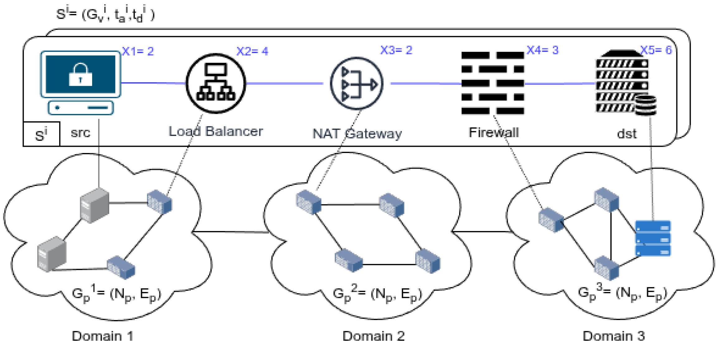
In this section, we describe the multi-domain system model and the corresponding problem formulation considered in this paper. We first introduce the SFC business model and then explain the substrate network model and the SFC model shown in Figure 1. The main symbols and notation used throughout the system model and problem formulation are summarized in

Table 3. List of Symbols and Notation.

Symbol	Description
$G_p$	Multi-domain Substrate Network
$N_p$	Set of Substrate Nodes
$E_p$	Set of Substrate Links
K	The number of Domains
$G_p^k$	A domain of Substrate Network
$N_p^k$	Set of Substrate Nodes in Domain k
$E_p^k$	Set of Substrate Links in Domain k
$e_{ij}^k$	Intra-domain Substrate Link Between Node $n_i^k$ and $n_j^k$
$e_{ij}^{k{k}^{\prime }}$	Inter-domain Substrate Link Between Node $n_i^k$ and $n_j^{k^{\prime }}$
$X_{n_j^k}^m$	Maximum Substrate Node Resource Capacity of $n_j^k$
$X_{n_j^k}^a$	Available Substrate Node Resource Capacity of $n_j^k$
$D_{e_{ij}^k}$	Intra-domain link propagation delay of link $e_{ij}^k$
$D_{e_{ij}^{k{k}^{\prime }}}$	Inter-domain link propagation delay of link $e_{ij}^{k{k}^{\prime }}$
$\mathcal{S}$	Set of requested SFCs
$s^l$	l-th requested SFC
$t_a^l$	Arrival time of l-th SFC
$t_d^l$	Departure time of l-th SFC
$G_v^l$	topology of l-th SFC
$v_i^l$	i-th VNF from l-th SFC
$x_{v_i^l}$	Resource requirement of VNF $v_i^l$
$d_{n_j^k}^{v_i^l}$	Node processing delay of l-th VNF deployed at Substrate Node $n_j^k$
${\xi }_{n_j^k}^{v_i^l}$	Intention of a VNF $v_i^l$ can be deployed to Substrate Node $n_j^k$, ${\xi }_{n_j^k}^{v_i^l}=\{0,1\}$
${\varphi }_{v_i^l}^{n_j^k}$	Whether $v_i^l$ is deployed on $n_j^k$
${\phi }_p^{v_i^l{v}_j^l}$	Whether virtual link between $v_i^l$ and $v_j^l$ is deployed to Substrate Path p
${\varrho }_{n_j^k}$	Resource utilization of Substrate Node $n_j^k$
${\rho }_{N_p}$	Resource utilization for all Substrate Nodes in $N_p$
$r(\delta \mid s,a)$	Reward by deployment intention $\xi$
$D_{s^l}$	End-to-end delay of SFC $s^l$
$O_{end}^{Ds}$	SFC end-to-end delay normalization
$r(\rho \mid s,a)$	Reward for refraining from reiterating the same Substrate Node selection
$r(s,a)$	Reward from the state s performing action a
B	Number of VNFs in a batch

. Finally, we present the problem formulation, including the objective function and the associated constraints.

3.1. SFC Business Model

The SFC business model considered in this paper consists of service providers (SPs), a virtual network operator (VNO), and infrastructure providers (InPs). Service providers (SPs) request network services in the form of SFCs. The VNO manages incoming SFC requests and coordinates their deployment. InPs maintain the substrate network within their respective administrative domains.

3.2. Substrate Network Model

We consider a multi-domain substrate network represented by an undirected graph

$$G_p=(N_p,E_p),$$

(1)

where $N_p$ denotes the set of all substrate nodes and $E_p$ denotes the set of all substrate links. The infrastructure is divided into K administrative domains. Each domain $k\in \{1,\dots ,K\}$ is modeled as a subgraph

$$G_p^k=(N_p^k,E_p^k),$$

(2)

where $N_p^k\subseteq N_p$ and $E_p^k\subseteq E_p$ denote the sets of substrate nodes and intra-domain links belonging to domain k, respectively. We denote by $e_{ij}^k$ the substrate link between two nodes within the same domain k, and by $e_{ij}^{k{k}^{\prime }}$ the substrate link connecting nodes in two different domains k and $k^{\prime }$. The associated propagation delays are given by $D_{e_{ij}^k}$ and $D_{e_{ij}^{k{k}^{\prime }}}$, respectively. Each substrate node $n_j^k$ in the domain k has a maximum resource capacity $X_{n_j^k}^m$ and an available capacity that varies over time $X_{n_j^k}^a\le X_{n_j^k}^m$.

3.3. SFC Model and Dynamic Request

We model the set of requested SFCs as

$$\mathcal{S}=\{s^1,s^2,\dots \},$$

(3)

where $s^l$ denotes the l-th SFC requested by a SP. Each SFC $s^l$ is characterized by its arrival time $t_a^l$ and departure time $t_d^l$, which together define its active lifetime within the system.

The internal structure of SFC $s^l$ is represented by a linear graph

$$G_v^l=(V_v^l,E_v^l),$$

(4)

where $V_v^l$ denotes the set of VNFs in $s^l$, and $E_v^l$ denotes the set of virtual links in $s^l$. The i-th VNF in $s^l$ is denoted by $v_i^l\in V_v^l$ and requires a certain amount of resources $x_{v_i^l}$ (e.g., CPU). When $v_i^l$ is deployed on the substrate node $n_j^k$ belonging to domain k, the processing delay incurred by this node is denoted by $d_{n_j^k}^{v_i^l}$. Therefore, each SFC $s^l$ specifies an ordered VNFs chain and service requirements that must be met by embedding the VNFs in substrate nodes and mapping virtual links in substrate paths. SFC requests arrive dynamically over time.

3.4. Problem Formulation

Based on the above models, we now present the problem formulation of the multi-domain SFC deployment problem. This formulation includes performance metrics, decision variables, an objective function, and constraints.

3.4.1. Performance Metrics

To evaluate the effectiveness of the proposed system, we consider the following metrics.

(a)

Acceptance Ratio.

The acceptance ratio measures the proportion of successfully embedded SFC among all SFC requests:

$$\begin{array}{c}\hfill \mathrm{AC}\_\mathrm{Ratio}={\displaystyle \frac{|{\mathcal{S}}_{\mathrm{suc}}|}{\left|\mathcal{S}\right|}},\end{array}$$

(5)

where $S_{\mathrm{suc}}$ denotes the set of successfully deployed SFCs. An SFC is considered successfully embedded if all VNFs and their associated virtual links are deployed without violating the resource constraints of the substrate nodes $N_p$.

(b)

End-to-End Delay.

The end-to-end delay $D_{s^l}$ quantifies the total latency experienced by SFC $s^l$ after deployment [11]. It consists of:

• Communication delay, including queueing, transmission, and propagation delays on intra-domain and inter-domain substrate links $e_{ij}^k$ and $e_{ij}^{k{k}^{\prime }}$ [11,35];
• Processing delay, represented by $d_{n_j^k}^{v_i^l}$, accounting for the time required for node $n_j^k$ to process VNF $v_i^l$ [11,35].

(c)

Resource Utilization.

Resource utilization characterizes the proportion of substrate node capacity that is being used. For a substrate node $n_j^k$ in the domain k, its utilization is represented as

$$\begin{array}{c}\hfill {\varrho }_{n_j^k}={\displaystyle \frac{{\sum }_{v_i^l\in V_{n_j^k}}{x}_{v_i^l}}{X_{n_j^k}^m}}\end{array}$$

(6)

where $V_{n_j^k}$ denotes the set of VNFs that are currently deployed on the substrate node $n_j^k$. The average utilization across all substrate nodes is then given by

$$\begin{array}{c}\hfill {\rho }_{N_p}={\displaystyle \frac{1}{|N_p|}}\sum _{n_j^k\in N_p}{\varrho }_{n_j^k}.\end{array}$$

(7)

3.4.2. Decision Variable

The actual embedding decisions are modeled using the following binary decision variables:

• VNF-to-substrate-node mapping:

  $${\varphi }_{v_i^l}^{n_j^k}=\left\{\begin{array}{cc}1,\hfill & \mathrm{if}\mathrm{VNF}{v}_i^l\mathrm{is}\mathrm{deployed}\mathrm{on}\mathrm{substrate}\mathrm{node}{n}_j^k,\hfill \\ 0,\hfill & \mathrm{otherwise}.\hfill \end{array}\right.$$

  (8)
• Virtual-link-to-substrate-path mapping:

  $${\phi }_p^{v_i^l{v}_j^l}=\left\{\begin{array}{cc}1,\hfill & \mathrm{if}\mathrm{the}\mathrm{virtual}\mathrm{link}\mathrm{between}{v}_i^l\mathrm{and}{v}_j^l\hfill \\ \hfill & \mathrm{is}\mathrm{routed}\mathrm{through}\mathrm{substrate}\mathrm{path}p,\hfill \\ 0,\hfill & \mathrm{otherwise}.\hfill \end{array}\right.$$

  (9)
• SFC acceptance variable:

  $$y_l=\left\{\begin{array}{cc}1,\hfill & \mathrm{if}\mathrm{SFC}\mathrm{request}{s}_l\mathrm{is}\mathrm{accepted},\hfill \\ 0,\hfill & \mathrm{otherwise}.\hfill \end{array}\right.$$

  (10)

3.4.3. Objective Function

The primary objective in practical multi-domain SFC deployment is to accommodate the maximum number of SFC requests while preserving the quality of the accepted services. Consequently, the goal function must explicitly account for both the quantity of accepted SFC requests and the end-to-end delay of the approved services. If the formulation just reduces the end-to-end delay, it may result in cautious placement selections that dismiss several SFC requests. Conversely, if the formulation just prioritizes the maximization of accepted SFCs requests, the accepted SFCs may incur significant end-to-end delays. Therefore, the goal function must equilibrate the acceptance of the SFC and the end-to-end delay.

Although resource utilization is a critical performance metric, as delineated in (6) and (7), direct optimization of resource utilization might require comprehensive information on the status of the resources, including node capacity, available resources, and current resource utilization. Revealing such information may contradict the privacy-preserving framework. Consequently, resource consumption remains an assessment measure, although the goal function emphasizes maximizing acceptability and minimizing delay.

Consequently, we introduce the binary acceptance variable $y_l$, where $y_l=1$ indicates that the SFC request $s_l$ is accepted and $y_l=0$ otherwise. The objective function is formulated as follows.

$$\underset{\{\varphi ,\phi ,y\}}{\max }\left(\lambda \sum _{s_l\in \mathcal{S}}{y}_l-\gamma \sum _{s_l\in \mathcal{S}}{y}_l{D}_{s_l}\right),$$

(11)

where $D_{s_l}$ denotes the end-to-end delay of the SFC request $s_l$, and $\lambda$ and $\gamma$ are weighting coefficients that control the trade-off between acceptance maximization and delay minimization. The term $y_l{D}_{s_l}$ ensures that the delay penalty is applied only to accepted SFC requests. In practice, $D_{s_l}$ can be normalized so that the acceptance and delay terms are comparable in the scalarized objective.

3.4.4. Constraints

The embedding decisions must satisfy the following constraints to ensure a valid and conflict-free deployment. Since SFC requests arrive and depart dynamically, the resource capacity constraint is imposed at each deployment decision time. Let $\mathcal{T}$ denote the set of deployment decision times, and let ${\mathcal{S}}_c\left(t\right)$ denote the set of accepted SFC requests that are currently deployed at time t.

(a)

Node Capacity Constraint.

For each substrate node, the total resource demand of all VNFs deployed on that node must not exceed its maximum capacity at any deployment decision time:

$$\begin{array}{c}\hfill \sum _{s_l\in {\mathcal{S}}_c\left(t\right)}\sum _{v_i^l\in N_v^l}{x}_{v_i^l}{\varphi }_{v_i^l}^{n_j^k}\left(t\right)\le X_{n_j^k}^m,\forall n_j^k\in N_p,\forall t\in \mathcal{T}.\end{array}$$

(12)

(b)

VNF Mapping Constraint.

Each VNF of an accepted SFC must be embedded on exactly one substrate node, whereas rejected SFCs are not mapped. This condition is enforced using the binary acceptance variable $y_l$:

$$\begin{array}{c}\hfill \sum _{n_j^k\in N_p}{\varphi }_{v_i^l}^{n_j^k}=y_l,\forall v_i^l\in N_v^l,\forall s_l\in \mathcal{S}.\end{array}$$

(13)

If $y_l=1$, the VNF $v_i^l$ must be assigned to exactly one substrate node. If $y_l=0$, no substrate node is selected for that VNF.

(c)

Virtual Link Mapping Constraint.

Similarly, each virtual link of an accepted SFC must be mapped onto exactly one substrate path connecting the substrate nodes that host the corresponding VNFs, whereas no path is selected for rejected SFCs:

$$\begin{array}{c}\hfill \sum _{p\in P_{n\left(v_i^l\right),n\left(v_j^l\right)}}{\phi }_p^{v_i^l{v}_j^l}=y_l,\forall (v_i^l,v_j^l)\in E_v^l,\forall s_l\in \mathcal{S}.\end{array}$$

(14)

where $P_{n\left(v_i^l\right),n\left(v_j^l\right)}$ denotes the set of candidate substrate paths between the substrate node hosting $v_i^l$ and the substrate node hosting $v_j^l$.

In summary, the multi-domain SFC deployment problem consists of finding ${\varphi }_{v_i^l}^{n_j^k}$, ${\phi }_p^{v_i^l{v}_j^l}$, and $y_l$ that satisfy the constraints (12)–(14) and optimize the objective function in (11).

4. Proposed Method

This section presents the proposed the $\mathcal{B}$-Batch mechanism for privacy-preserving multi-domain SFC deployment. We first revisit PPDM and its limitations and then describe the proposed mechanism.

4.1. PPDM Overview and Limitations

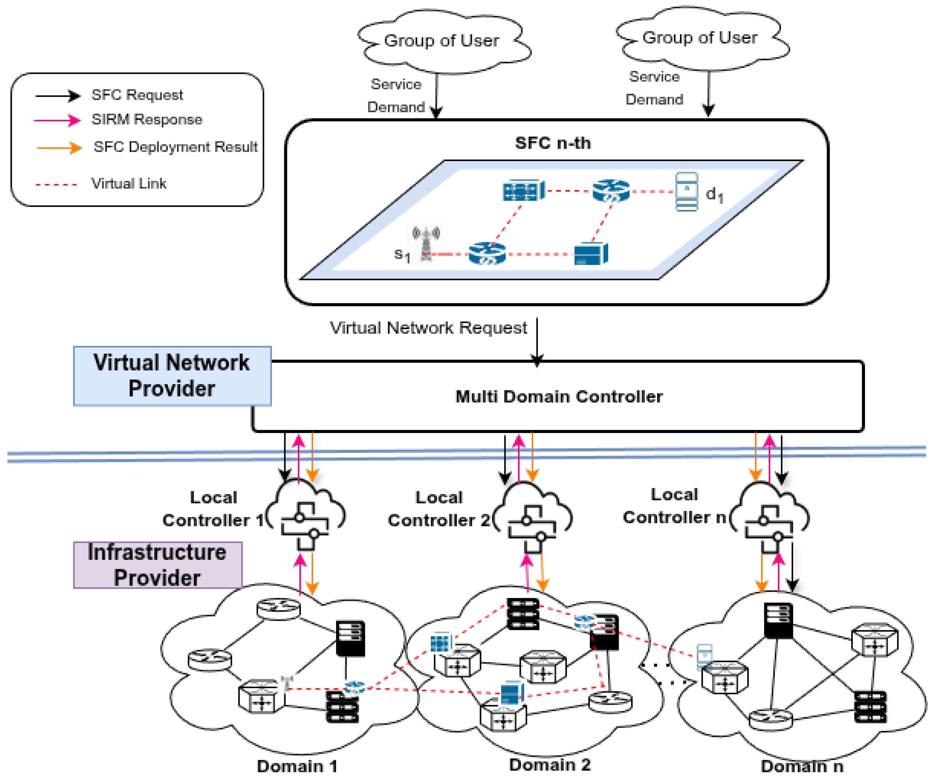
PPDM [11] adopts the hierarchical SFC deployment architecture (Figure 2) to preserve domain privacy. The architecture consists of two layers: a centralized Multi-Domain Controller (MDC) and multiple Local Controllers (LCs). The MDC, which is operated by the VNO, coordinates the end-to-end deployment of the SFC across multiple domains. Each LC, which is operated by the respective InP, is responsible for deploying VNFs and virtual links in the requested SFC within the domain. In order to preserve domain privacy, detailed substrate-level information is not shared among MDC and LC; instead, abstracted resource information called the Service Intention Response Matrix (SIRM) is shared among them. SIRM is a binary matrix where the (i, j) element ${\xi }_{n_j^k}^{v_i^l}$ takes the value 1 if VNF $v_i^l$ can be deployed on the substrate node $n_j^k$, and 0 otherwise.

Figure 3 illustrates the PPDM deployment procedure. When an SFC request arrives, the MDC distributes the request to all LCs. Each LC evaluates the feasibility of mapping VNFs onto its local substrate nodes based on its private resource information. Specifically, each LC constructs the corresponding elements of the SIRM, where ${\xi }_{n_j^k}^{v_i^l}\in \{0,1\}$ indicates whether a substrate node $n_j^k$ can host VNF $v_i^l$. These SIRM elements are then returned to the MDC and aggregated into a global SIRM. The MDC subsequently feeds this SIRM to the DQN agent, which selects a substrate node for each VNF in the SFC. The corresponding virtual links are then mapped onto the shortest paths in the substrate network.

A key characteristic of PPDM is that the feasibility of all VNFs in the SFC must be evaluated before the final decision on the deployment of the SFC is made. During this SIRM construction stage, whenever a substrate node is deemed capable of hosting a VNF, the required resources are temporarily reserved, even though the final deployment has not yet been determined. This temporary reservation is referred to as virtual occupation.

To reduce unnecessary evaluation and limit the number of candidate nodes, PPDM applies a top-$\eta$ node selection strategy, where only a subset of candidate nodes with higher capacity is considered. Although this approach helps reduce the number of evaluated nodes, it does not eliminate the effect of virtual occupation.

Because all VNFs are evaluated in advance, a single substrate node can reserve resources for multiple VNFs simultaneously. As a result, the effective capacity observed during the evaluation stage can be significantly lower than the actual physical capacity available after deployment. The available resources of the substrate node $n_j^k$ when evaluating the feasibility of VNF $v_i^l$ are expressed as

$$\begin{array}{c}\hfill X_{n_j^k}^a=X_{n_j^k}^m-\sum _{v_m^l\in N_d}{\xi }_{n_j^k}^{v_m^l}·x_{v_m^l}-\sum _{v_q^o\in N_c}{\varphi }_{v_q^o}^{n_j^k}·x_{v_q^o}\end{array}$$

(15)

where $N_d$ is the set of VNFs whose feasibility has already been evaluated within the current SFCs and $N_c$ is the set of VNFs belonging to the SFCs that are currently operating.

As provisional reservations in the second term accumulate, the remaining capacity observed during evaluation may become significantly smaller than the actual capacity available after the final deployment. Consequently, later VNFs may be incorrectly classified as infeasible, even though sufficient resources would exist if temporary reservations were released. This effect is reflected in the SIRM, where the feasibility indicators ${\xi }_{n_j^k}^{v_i^l}$ tend to become zero for all candidate substrate nodes. This situation is referred to as an ambiguous state, where no candidate node is marked as feasible (i.e., ${\xi }_{n_j^k}^{v_i^l}=0$ for all $n_j^k$). As a result, the DQN agent receives a degraded state representation with no feasible options, making it difficult to identify valid deployment decisions. This increases the likelihood of deployment failure and ultimately reduces the overall acceptance ratio achieved by PPDM.

4.2. $\mathcal{B}$-Batch Sequential Deployment Mechanism

As discussed earlier, PPDM evaluates the feasibility of an entire SFC in a single orchestration round. Consequently, each LC must maintain virtual reservations for all feasible VNFs throughout the orchestration cycle. This design results in cumulative virtual occupation across domains, which can significantly distort perceived resource availability.

To address this limitation, we propose the $\mathcal{B}$-Batch mechanism which evaluates the feasibility of $\mathcal{B}$ consecutive VNFs rather than the entire SFC. For each domain k, the LC computes and returns a compact batch-based SIRM. As a result, only VNFs within the current batch contribute to temporary resource reservations, thereby reducing both the magnitude and the duration of virtual occupation within the domain.

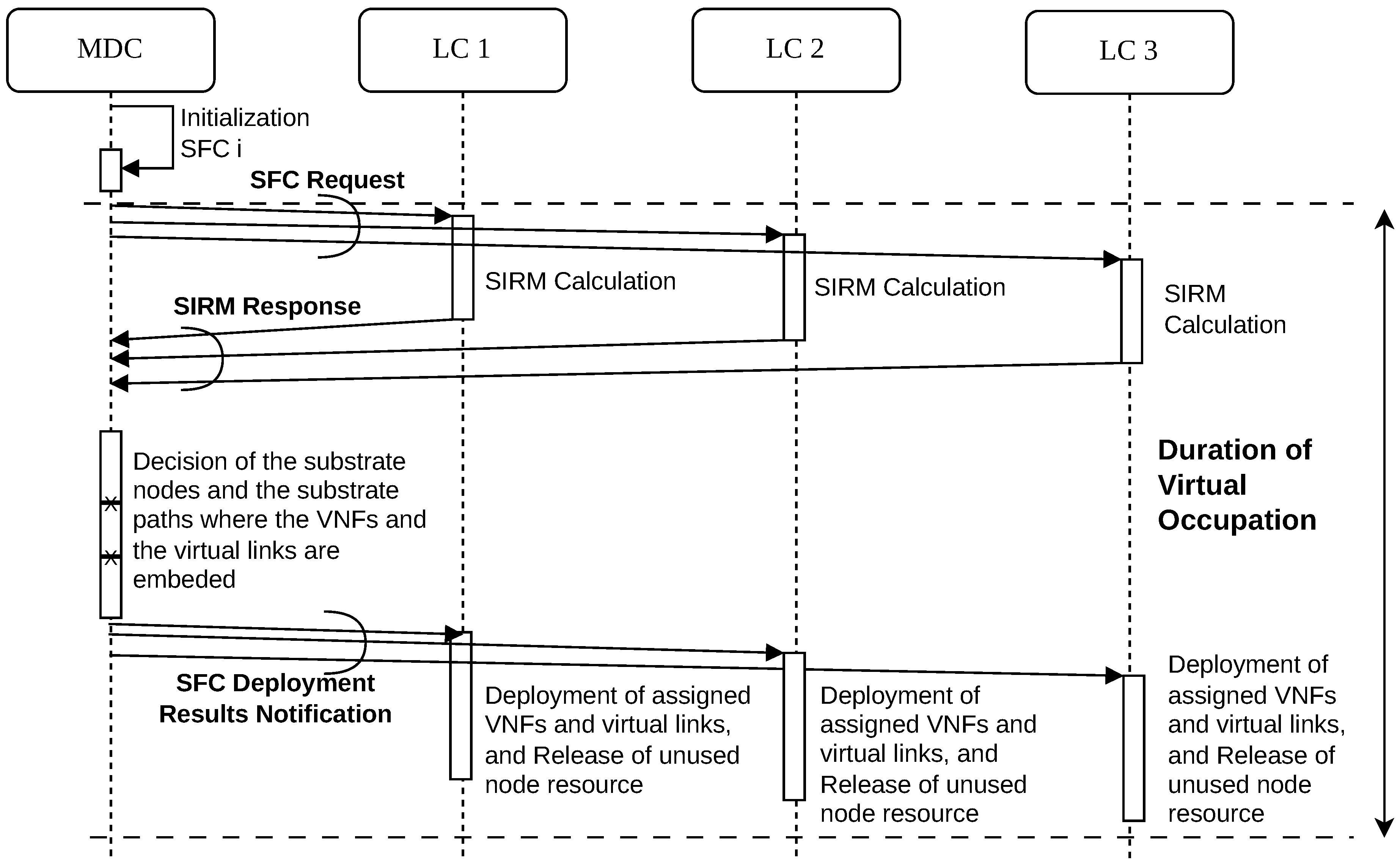
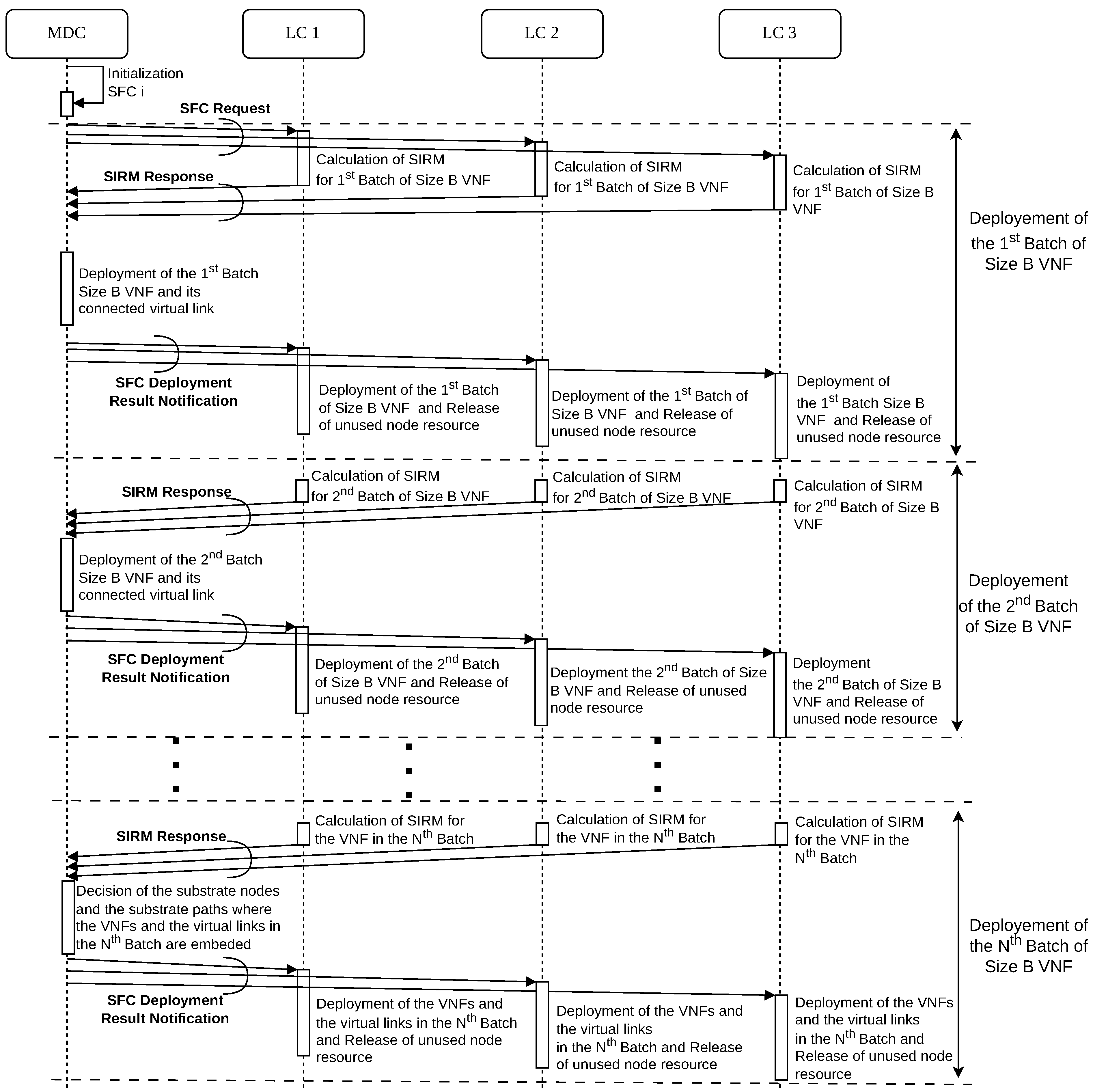
Figure 4 illustrates the general deployment procedure of the proposed the $\mathcal{B}$-Batch mechanism. When the MDC receives an SFC request, the complete SFC information is sent once to all LCs during the initialization phase. This information includes the SFC request identifier, VNF resource requirements, virtual link structure, and service ordering information.

After receiving the SFC request, each LC evaluates the feasibility of the VNFs according to the current batch identifier. For the current batch, the LC performs a local feasibility evaluation using its internal topology and resource information. Temporary resource reservations, referred to as virtual occupation, are applied only to VNFs within the current batch. Based on this evaluation, each LC constructs and returns a batch-level SIRM response to the MDC. The SIRM only contains binary feasibility indicators ${\xi }_{n_j^k}^{v_i^l}\in \{0,1\}$, where $\xi =1$ indicates that the substrate node $n_j^k$ can feasibly host VNF $v_i^l$, and $\xi =0$ otherwise.

Based on the SIRM responses received, the MDC estimates the predicted resource condition of the substrate nodes and ranks the feasible nodes. The MDC then selects the top-$\eta$ candidate nodes from the feasible SIRM entries and uses the resulting candidate set as the input to the DQN-based node selection process. This candidate selection strategy follows the general SIRM-based orchestration principle, where the MDC makes deployment decisions using feasibility indicators rather than detailed domain-internal resource information. In this study, top-$\eta$ selection is performed at the MDC to support global candidate comparison across multiple domains.

After the DQN determines the deployment decision for the VNFs in the current batch, the MDC sends the selected deployment result to the corresponding LC. The deployment notification includes control information such as the request ID (req_id), batch ID (sub_sfc_id), acknowledgment flag (ack), selected substrate-node mapping, and the next batch identifier. These identifiers are used to track the progress of deployment, synchronize batch-by-batch execution, and support rollback if a later batch fails.

Upon receiving the deployment notification, the corresponding LC performs the actual VNF deployment on the selected substrate nodes and releases unused virtual occupations from the current batch. If the deployment succeeds, the LC sends a success notification to the MDC together with the identifier of the next batch to be processed. This procedure continues until all batches of the SFC are successfully deployed. If a later batch fails, the MDC triggers a rollback for previously deployed batches and marks the SFC request as rejected.

Compared to PPDM, which performs a single SIRM exchange for the entire SFC, the proposed method introduces multiple SIRM exchanges in batches. This increases the signaling frequency, as multiple rounds of interaction between the MDC and the LC are required. However, each exchange involves fewer VNFs, resulting in a smaller feasibility evaluation at each step.

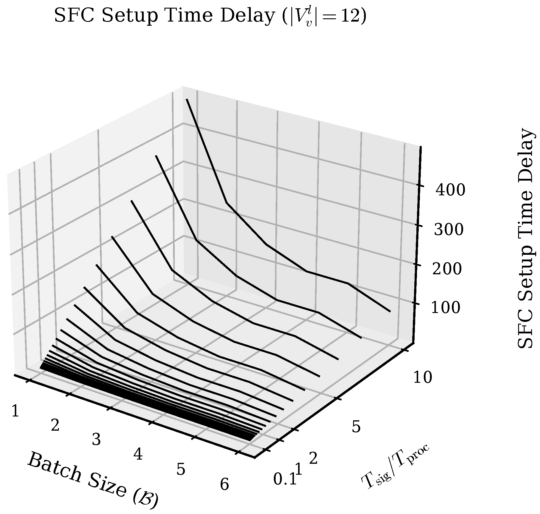
The total number of orchestration rounds depends on the batch size B. Smaller batch sizes result in more rounds, leading to a longer deployment setup time but more accurate feasibility evaluation. In contrast, larger batch sizes reduce the number of orchestration rounds, which can shorten the overall deployment setup time at the cost of reduced feasibility accuracy.

Under the proposed the $\mathcal{B}$-Batch mechanism, the virtual occupation is confined to the VNFs within the current batch, resulting in a smaller and shorter virtual occupation. Consequently, the effective available capacity of the substrate node $n_j^k$ during the feasibility evaluation is given by:

$$\begin{array}{c}\hfill X_{n_j^k}^a=X_{n_j^k}^m-\sum _{v_m^l\in N_{\mathcal{B}}}{\xi }_{n_j^k}^{v_m^l}·x_{v_m^l}-\sum _{v_u^l\in N_{\mathcal{E}}}{\varphi }_{v_u^l}^{n_j^k}·x_{v_u^l}-\sum _{v_q^o\in N_c}{\varphi }_{v_q^o}^{n_j^k}·x_{v_q^o},\end{array}$$

(16)

where $N_{\mathcal{B}}$ denotes the set of VNFs within the current batch whose feasibility has been evaluated, $N_{\mathcal{E}}$ denotes the set of VNFs in the current SFC that have already been deployed before the current batch, and $N_c$ denotes the set of VNFs belonging to SFC that are currently in operation. Note that the second term on the RHS represents the virtual occupation within the current batch, which is reduced compared to the virtual occupation over the entire SFC. The third and fourth terms represent the actual resource consumption of VNFs that have already been deployed in the current SFC and those belonging to active SFCs, respectively.

The proposed mechanism preserves privacy by limiting the information exchanged between the MDC and the LC. Each LC evaluates batch feasibility using its own local information, such as available resources, internal topology, and routing conditions. However, these detailed data are not shared with the MDC. The LC only returns binary SIRM feasibility indicators, which show whether a candidate substrate node can support a specific VNF in the current batch. Therefore, the MDC can make deployment decisions without knowing exact residual resources, internal topology, link states, or routing paths. However, because SIRM responses are exchanged repeatedly, the MDC may still observe coarse feasibility trends over time. For example, if a node is frequently feasible or becomes infeasible across several requests, the MDC may infer general resource availability or congestion. Thus, the proposed mechanism prevents direct disclosure of sensitive domain information, while repeated binary responses may still provide limited indirect information.

4.3. SFC Batch Partitioning

For the deployment decision process, the MDC sorts the VNFs based on their resource requirements in descending order. This sorting is used only to prioritize VNFs with higher resource demands during node selection. It does not change the logical service chain according to the original service chain in order of the SFC. The sorted VNF sequence is denoted as

$${\tilde{V}}^l=\{{\tilde{v}}_1^l,{\tilde{v}}_2^l,\dots ,{\tilde{v}}_{|V_v^l|}^l\},$$

where

$$x_{{\tilde{v}}_1^l}\ge x_{{\tilde{v}}_2^l}\ge \cdots \ge x_{{\tilde{v}}_{|V_v^l|}^l},$$

After sorting, the MDC partitions the sorted VNF sequence into fixed-size batches. The r-th batch of the l-th SFC request is defined as

$${\mathcal{B}}_r^l=\left\{{\tilde{v}}_{(r-1)\mathcal{B}+1}^l,{\tilde{v}}_{(r-1)\mathcal{B}+2}^l,\dots ,{\tilde{v}}_{\min (r\mathcal{B},|V_v^l\left|\right)}^l\right\},$$

where $r=1,2,\dots ,⌈|V_v^l|/\mathcal{B}⌉$ and $\mathcal{B}$ denotes the batch size. During the initialization phase, the MDC sends the complete SFC request only once to all LCs. This request includes the original service chain order, the VNF resource requirements, the virtual link structure, and the batch identifiers. After this initial transmission, the deployment process is coordinated batch-by-batch using the corresponding batch identifier.

The size of the batch $\mathcal{B}$ controls the granularity of the deployment process. A smaller $\mathcal{B}$ creates more batches and enables a finer-grained feasibility evaluation. This reduces the duration and magnitude of virtual occupation but increases the number of orchestration rounds. In contrast, a larger $\mathcal{B}$ reduces the number of orchestration rounds and signaling overhead, but may produce a coarser feasibility representation and increase the ambiguity of SIRM. Finally, after all VNFs have been mapped to substrate nodes, virtual links are routed according to the original service chain.

4.4. DRL Agent for Batch Deployment

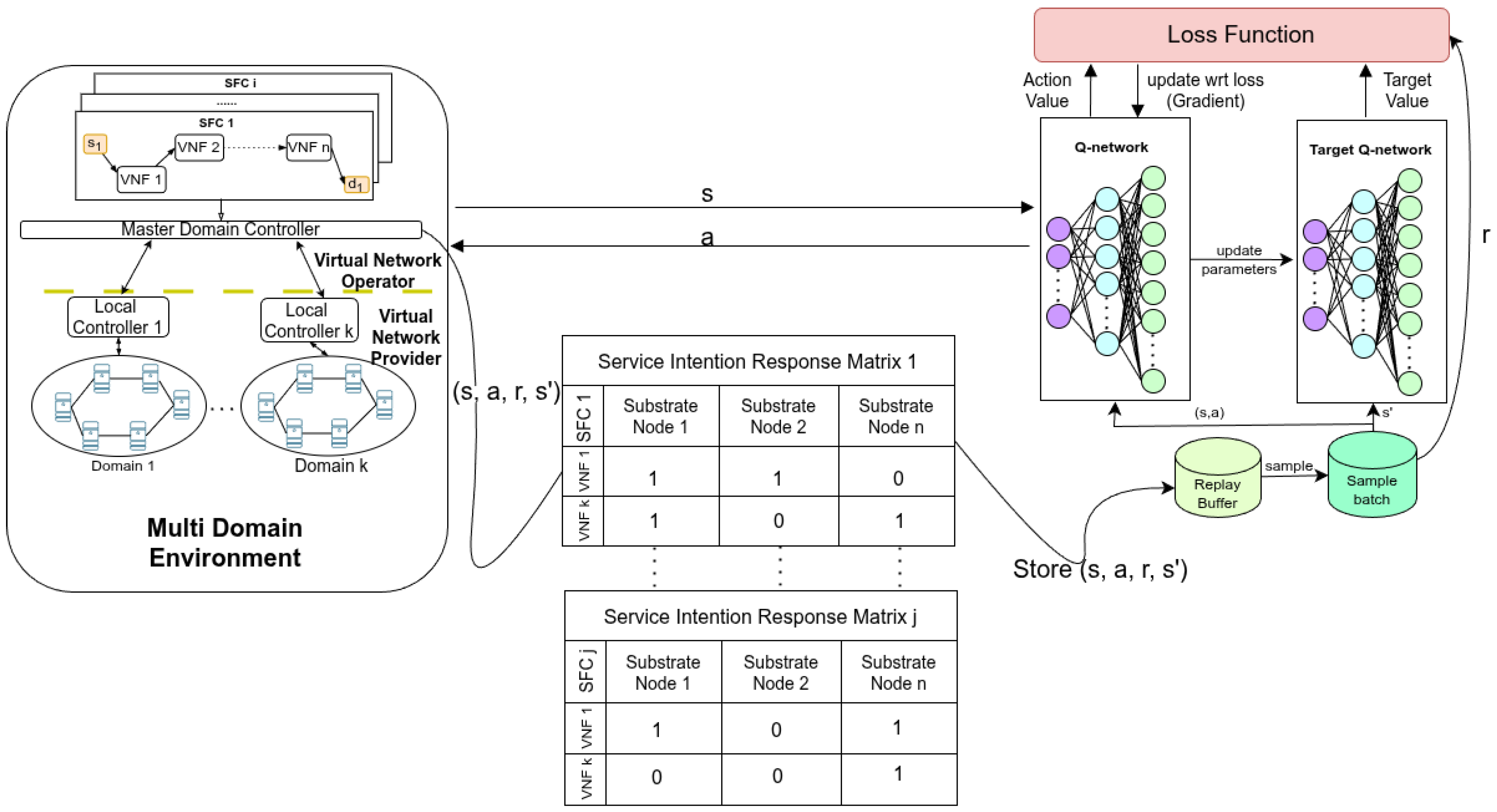
Figure 5 illustrates the DQN-based learning framework adopted for the proposed the $\mathcal{B}$-Batch mechanism. The general DRL formulation follows the conventional approach introduced in [11], while our contribution focuses on the proposed the $\mathcal{B}$-Batch mechanism. In this architecture, the multi-domain substrate network together with the proposed $\mathcal{B}$-Batch mechanism forms the environment, while the MDC acts as learning agents. At each decision step, the agent observes the state $s_t$ derived from the batch-level SIRM and selects an action $a_t$ corresponding to the deployment of a single VNF onto a substrate node. This sequential decision process continues until all VNFs in the current batch are deployed.

The state $s_t$ corresponds to the feasibility information at the batch level represented by the SIRM, which preserves domain privacy by providing the agent only with feasibility indicators rather than fine-grained substrate resource details; once the SIRM ${\xi }_{n_j^k}^{v_i^l}$ for all VNFs in the batch is constructed, the DQN agent sequentially uses each row corresponding to VNF $v_i^l$, containing feasibility information across all substrate nodes, as the state input to determine the deployment action.

The action $a_t$ represents the selection of a substrate node for the current VNF within the batch. The action space is discrete, and its size corresponds to the total number of substrate nodes in all domains. This design ensures that the agent operates in a finite action space. After all VNFs in the batch are deployed, the corresponding virtual links between the selected substrate nodes are activated. are routed using the shortest-path method.

The Q-network is implemented as a fully connected feedforward neural network that approximates the action-value function $Q(s_t,a_t)$. As shown in Figure 5, the size of the input layer is equal to the state dimension, denoted by state_size, where state_size corresponds to the total number of substrate nodes in all domains. The network then processes the input through several hidden layers. The output layer contains action_size neurons, where action_size corresponds to the total number of substrate nodes in all domains. Each output neuron represents the Q-value of selecting one substrate node for the current VNF.

The reward function adopted in this environment follows the formulation proposed in [11] and is defined as:

$$r_t=r(\delta \mid s_t,a_t)+\alpha ·{\rho }_{N_p,t}+\beta ·\left(O_{end,t}^{Ds}r(\rho \mid s_t,a_t)\right).$$

(17)

where each term captures a distinct system objective: (i) the feasibility reward $r(\delta \mid s_t,a_t)$, which reflects the SIRM-based feasibility result for the current VNF; (ii) the global substrate utilization term $\alpha ·{\rho }_{N_p,t}$, which encourages efficient resource usage based on node utilization; (iii) the delay-related term $\beta ·O_{end,t}^{Ds}$, which emphasizes the end-to-end delay performance; and (iv) the repetition penalty $r(\rho \mid s_t,a_t)$, which discourages repeated node selections.

It should be noted that the proposed DQN model uses a fixed-dimensional SIRM-based state representation and a discrete action space corresponding to the candidate substrate nodes. Therefore, the model is trained with a specific network configuration. If the number and ordering of substrate nodes remain unchanged, the input and output dimensions of the DQN model are preserved, and the trained model can still be applied to updated resource availability or traffic conditions represented through the SIRM. However, when the number of domains or the number of substrate nodes changes significantly, the state and action spaces can also change, which can affect the performance of the trained model. In such cases, partial or complete retraining may be required.

The Algorithm 1 summarizes the general training and deployment procedure of the proposed $\mathcal{B}$-batch mechanism. For each SFC request arriving, the VNF chain is partitioned into fixed-size batches, and the VNFs within each batch are processed sequentially. At each decision step, the environment constructs the SIRM and provides the corresponding state $s_t$ to the DQN agent, which selects an action $a_t$ corresponding to the deployment of the current VNF. The environment then executes the action, updates the availability of resources, and computes the reward $r_t$. If any VNF within a batch cannot be successfully deployed, the entire SFC request is rejected; otherwise, the process continues until all batches are successfully deployed. When each SFC deployed reaches its expiration time, the resources allocated to the expired SFC are released.

The agent is trained using the standard DQN framework. After executing the action $a_t$ in state $s_t$, the transition tuple $(s_t,a_t,r_t,s_{t+1})$ is stored in the replay buffer. When sufficient samples are available, a mini-batch is drawn to update the Q-network. For each sampled transition, the target value is computed as

$$y=r_t+\gamma \underset{a^{\prime }}{\max }\overline{Q}(s_{t+1},a^{\prime }),$$

(18)

where $\overline{Q}(·)$ denotes the target network and $\gamma$ is the discount factor. The Q-network parameters $\theta$ are updated by minimizing the temporal-difference loss

$$L\left(\theta \right)=\mathbb{E}\left[{(Q(s_t,a_t\mid \theta )-y)}^2\right],$$

(19)

using stochastic gradient descent. This optimization step reduces the discrepancy between the predicted and target Q-values, thus improving future action selection.

Algorithm 1 $\mathcal{B}$-Batch Sequential Deployment Mechanism for Multi-Domain SFCs

Input:  Set of SFC requests $\mathcal{S}$ Output:  Deployment decisions and trained DQN policy 1: Initialize Q-network $Q(·;\theta )$, target network $\overline{Q}(·;\overline{\theta })$, and replay buffer $\mathcal{D}$. 2: for each episode $e=1,2,\dots ,E$ do 3:       Reset environment and substrate resource state. 4:       for each arriving SFC request $s^l\in \mathcal{S}$ do 5:             Partition the VNF chain of $s^l$ into fixed batches $\{{\mathcal{B}}_1,{\mathcal{B}}_2,\dots \}$. 6:             $\mathit{success}\leftarrow \mathbf{true}$ 7:             for each batch ${\mathcal{B}}_b$ of SFC $s^l$ do 8:                  Construct batch-level SIRM for the current batch. 9:                  for each VNF $v_i^l\in {\mathcal{B}}_b$ do 10:                       Extract state $s_t$ from the SIRM row of $v_i^l$. 11:                       Select action $a_t$ using an $ϵ$-greedy policy based on $Q(s_t,·;\theta )$. 12:                       Execute deployment according to $a_t$. 13:                       if deployment fails then 14:                             $\mathit{success}\leftarrow \mathbf{false}$ 15:                             break 16:                       end if 17:                       Compute total reward $$r_t=r(\delta \mid s_t,a_t)+\alpha {\rho }_{N_p,t}+\beta O_{end,t}^{Ds}r(\rho \mid s_t,a_t).$$ 18:                       Observe next state $s_{t+1}$ and terminal flag $d_t$. 19:                       Store transition $(s_t,a_t,r_t,s_{t+1})$ in replay buffer $\mathcal{D}$. 20:                       if $\left|\mathcal{D}\right|$ is sufficient then 21:                             Sample a mini-batch from $\mathcal{D}$. 22:                             Compute target $$y_t=\left\{\begin{array}{cc}{r}_t,\hfill & \mathrm{if}{d}_t=1,\hfill \\ r_t+\gamma \underset{a^{\prime }}{\max }\overline{Q}(s_{t+1},a^{\prime };\overline{\theta }),\hfill & \mathrm{otherwise}.\end{array}\right.$$ 23:                             Update Q-network by minimizing $$L\left(\theta \right)=\mathbb{E}\left[{\left(y_t-Q(s_t,a_t;\theta )\right)}^2\right].$$ 24:                       end if 25:                       Periodically update target network $\overline{Q}(·;\overline{\theta })$. 26:                  end for 27:                  if not $\mathit{success}$ then 28:                       Trigger rejection or rollback procedure for $s^l$. 29:                       break 30:                  end if 31:             end for 32:             if $\mathit{success}$ then 33:                  Accept SFC request $s^l$. 34:             else 35:                  Reject SFC request $s^l$. 36:             end if 37:       end for 38: end for

5. Experimental Setup

This section outlines the experimental environment used to evaluate the proposed Fixed $\mathcal{B}$-Batch Sequential Deployment mechanism. All baseline and proposed algorithms operate on the same multi-domain substrate network, observe identical traffic traces for each random seed, and follow a unified evaluation protocol. The setup covers the physical substrate configuration, the stochastic SFC generation model, the benchmark methods, the reinforcement learning training procedure, and the testing methodology.

5.1. Substrate Network Configuration

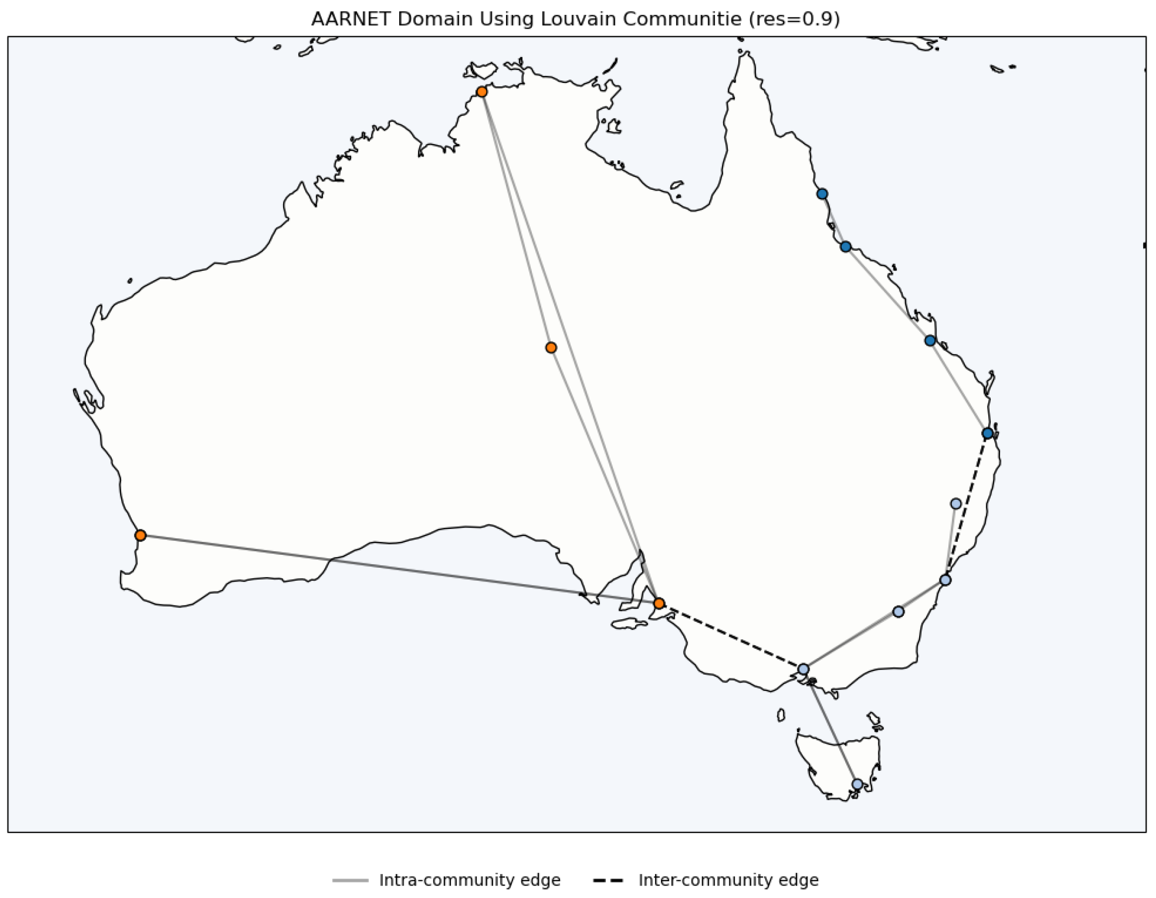
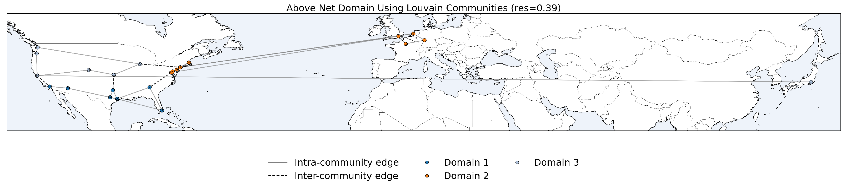
The substrate network is constructed from two real-world backbone topologies obtained from the Internet Topology Zoo: AARNET and AboveNet. The AARNET topology is used as the main evaluation topology, whereas AboveNet is used as an additional topology to verify whether the observed performance trends remain consistent under another substrate network structure. The detailed substrate node topologies of AARNET and AboveNet are provided in Appendix A, as shown in Figure A1 and Figure A2, respectively. The basic characteristics of the two topologies are summarized in

Table 4. Substrate network topologies used in the evaluation.

Topology	Number of Nodes	Number of Edges
AARNET	19	24
AboveNet	23	31

.

To emulate a multi-domain environment, each topology is divided into $K=3$ administrative domains using the Louvain community detection algorithm. For AARNET, the three domains are defined as follows:

$$D_1=\{1,4,5,6,7\},D_2=\{0,2,3,8,9,10,15,16\},D_3=\{11,12,13,14,17,18\}.$$

For AboveNet, the three domains are defined as follows:

$$D_1=\{0,1,4,5,6,7,8,9,12\},D_2=\{2,3,10,13,14,19,20\},D_3=\{11,15,16,17,18,21,22\}.$$

Each substrate node $n_j^k$ is assigned a computational capacity drawn from a random uniform distribution $U[7,19]$, representing normalized processing units. The available capacity $X_{n_j^k}^a$ is dynamically updated as VNFs are deployed and released during simulation. For both AARNET and AboveNet, link propagation delays are generated using the same uniform random delay settings, as summarized in

Table 5. Link Delay Settings in Multi-Domain Topology (Time Units).

Domain	Domain 1	Domain 2	Domain 3
Domain 1	U[5,10]	U[11,20]	U[21,30]
Domain 2	U[11,20]	U[5,10]	U[11,20]
Domain 3	U[21,30]	U[11,20]	U[5,10]

. Intra-domain links are assigned the lowest delay ranges, whereas links connecting more distant domains are assigned higher propagation-delay ranges. Using the same delay-generation settings for both topologies ensures that the comparison focuses on the effect of different substrate network structures rather than different delay configurations. These settings follow established practice in prior privacy-preserving SFC deployment studies. The substrate topology, domain partition, and link attributes remain fixed throughout the training and evaluation phases.

5.2. SFC Traffic and VNF Model

Incoming SFC requests follow a Markov-modulated Poisson process (MMPP), a two-state arrival model that captures the burstiness and temporal correlation typically observed in operational carrier and cloud networks. The arrival process alternates between a normal-load and a high-load state, in which the burst (high-load) regime produces approximately 50% denser arrivals than the low-load regime. This modulation enables the MMPP to capture realistic burstiness and workload variability beyond a stationary Poisson model.

Each SFC request comprises a sequence of VNFs whose length is selected using a uniform random generator across three categories. Short service chains contain between 3 and 6 VNFs, medium chains contain 6 to 9 VNFs, and long chains contain 9 to 12 VNFs. This distribution yields a representative blend of simple, moderate and complex SFCs, allowing a comprehensive evaluation of different embedding complexities.

For every VNF $v_i^l$, the computational demand and processing delay are drawn independently of uniform distributions: resource requirements of $U[2,8]$ and processing delays of $U[5,10]$. These randomized parameters emulate the heterogeneity of real deployments, where VNF workloads vary significantly in processing intensity and delay sensitivity. The SFC lifetimes follow an exponential distribution with rate parameter $\lambda =1$, a commonly used assumption in VNE and SFC orchestration studies. To ensure a fair comparison, all algorithms are evaluated using identical traffic traces for each experimental seed.

Although the experimental evaluation in this study focuses on sequential SFC chains, the SIRM-based feasibility-evaluation process is not inherently limited to linear chains. For a general SFC graph, each LC can still evaluate the feasibility of deploying the requested VNFs on its local substrate nodes and return the corresponding SIRM response without exposing internal topology or resource information. However, arbitrary SFC graphs require dependency-aware batch partitioning on the MDC side. In such cases, the MDC first determines a valid VNFs ordering or grouping based on the dependency relationships among VNFs and virtual links. The VNFs can then be partitioned into batches while preserving precedence constraints, and each batch can be processed using the same batch-level SIRM construction procedure.

5.3. Compared Algorithms

In this study, three deployment strategies are evaluated.

• PPDM. PPDM is implemented according to the corrected formulation presented in Section 4.1, incorporating capacity clamping, VNF-level reordering, and iterative top-$\eta$ candidate selection. Each domain computes its candidate set using $\eta =0.3|N_p^K|$.
• Exposing Privacy Deep Q-Network (EP-DQN). EP-DQN follows a similar learning framework to the PPDM algorithm, where the deployment strategy for SFCs is learned within a fully transparent network environment. Both the EP-DQN and the proposed approach employ the same DQN architecture to determine deployment decisions. However, EP-DQN utilizes detailed substrate resource information as input, which compromises domain privacy. In contrast, the proposed method replaces this information with the SIRM, enabling a fair comparison to evaluate the effectiveness of privacy-preserving decision-making in dynamic cross-domain SFC deployment.
• The $\mathcal{B}$-Batch Sequential Deployment Mechanism. The proposed approach groups the VNFs into batches, with batch sizes selected based on the length of the SFC, as shown in

  Table 6. Batch Size Settings for the Proposed $\mathcal{B}$-Batch Sequential Deployment Mechanism.

  SFC Length $|{\mathit{G}}_{\mathit{v}}^{\mathit{l}}|$	Allowed Batch Sizes $\mathcal{B}$
  Short SFCs	$1,2,3$
  Medium SFCs	$1,2,3,4,5$
  Long SFCs	$1,2,3,4,5,6$

  mitigating virtual occupation while maintaining compatibility with privacy-preserving constraints.

5.4. Training Settings

The reinforcement learning agent uses a DQN to solve the batch-based embedding task. For each substrate network, the training process consists of multiple episodes, where each episode contains 300 SFC arrival requests. During training, SFC requests are generated using an MMPP traffic model that alternates between normal-load and burst-load states, with mean interarrival times of 0.25 and 0.167 time units, respectively. The transition probability between the two states is set to $5\%$.

The Q-network consists of three fully connected layers with ReLU activation functions.

Table 7. DQN Hyperparameter Settings.

Parameter	Value
Discount factor $\gamma$	0.95
Learning rate	0.001
Optimizer	Adam
Q-network architecture	Fully connected (2 hidden layers: 256, 128 neurons, ReLU)
Input dimension	state_size
Output dimension	number of substrate nodes
Batch size	64
Replay buffer size	50,000
Initial exploration ${ϵ}_0$	1.0
Minimum exploration ${ϵ}_{\min }$	0.01
Decay schedule	${ϵ}_{t+1}=0.995{ϵ}_t$
Reward weights $(\alpha ,\beta )$	$(0.2,0.8)$
Normalization range	$[-1,1]$

summarizes the hyperparameters used during training. The state features related to substrate resource utilization ${\rho }_{N_p}$ and end-to-end delay $O_{end}^{Ds}\left(t\right)$ are normalized to the interval $[-1,1]$ to improve numerical stability. After the training reward becomes stable for each substrate network, the trained Q-network weights are saved and used for testing under different traffic conditions.

5.5. Testing Settings

System performance is evaluated under varying traffic loads by replacing the MMPP arrival process with fixed interarrival times. Following the normal-load and burst-load traffic regimes introduced earlier and also adopted in the training scenario, the testing considers a set of deterministic interarrival values for each regime. For the normal-load regime, the interarrival times are set to $\{1.5,0.75,0.375,0.25,0.125,0.0625\}$ time units. For the burst-load regime, the denser traffic conditions are modeled using interarrival times of $\{1.0,0.5,0.25,0.167,0.0833,0.0417\}$ time units. These configurations range from light to high-traffic operating conditions, enabling a comprehensive characterization of embedded performance across diverse workload intensities.

The Testing consists of 100 episodes, each containing 100 SFC arrivals, and is repeated under 10 independent random seeds. All SFC requests, including rejected arrivals, are included in the evaluation metrics to ensure an unbiased performance assessment.

5.6. Implementation Details

All simulations are implemented in Python using PyTorch 2.4.1 with CUDA 12.4, NetworkX 3.4, and NumPy 1.26. The experiments are executed on a workstation running Ubuntu 20.04.6 LTS, equipped with an Intel i9-9900K processor (5.0 GHz, 16 threads), an NVIDIA GeForce RTX 2080 Ti GPU, and 64 GB of RAM. Random seeds are fixed across all runs to ensure strict reproducibility.

6. Results and Analysis

This section evaluates the proposed $\mathcal{B}$-Batch mechanism from three complementary perspectives. First, we verify the training stability of all the mechanisms by observing the convergence of the rewards during the learning process. All models reach stable convergence after approximately 200 training episodes, indicating that the learned policies have stabilized. Second, we evaluated the performance of the testing under varying traffic loads, focusing on acceptance ratio, end-to-end delay, and substrate resource utilization. Third, we analyze the distribution of selected substrate nodes for each mechanism to assess load-balancing behavior. Finally, we analyze a normalized analytical approximation of the deployment setup time for the proposed system.

All mechanisms, PPDM, EP-DQN, and the $\mathcal{B}$-Batch mechanism operate under identical substrate topologies, traffic intensity settings, and VNF-generation patterns to ensure strict fairness. As outlined in the SFCs Traffic and VNF Model subsection, the results are reported separately for short, medium, and long SFCs to expose the impact of increasing embedding complexity. The detailed numerical results for the AARNET topology are provided in Appendix B, as shown in

Table A1. Acceptance Ratio (Mean ± Std) Across All Interarrival Times for Short SFCs in AARNET Topology.

Method	1.5	0.75	0.375	0.25	0.125	0.0625
PPDM	$98.90\pm 0.19$	$97.40\pm 0.31$	$92.69\pm 0.76$	$87.22\pm 1.11$	$71.86\pm 1.49$	$53.77\pm 1.47$
$\mathcal{B}$-Batch (B = 1)	$100\pm 0.0$	$100\pm 0.01$	$99.72\pm 0.05$	$98.35\pm 0.13$	$85.80\pm 0.66$	$60.87\pm 0.91$
$\mathcal{B}$-Batch (B = 2)	$99.38\pm 0.16$	$99.18\pm 0.16$	$98.18\pm 0.22$	$95.86\pm 0.52$	$82.50\pm 1.33$	$59.79\pm 1.53$
$\mathcal{B}$-Batch (B = 3)	$99.55\pm 0.12$	$98.79\pm 0.14$	$96.28\pm 0.45$	$92.53\pm 0.82$	$78.34\pm 1.39$	$57.57\pm 1.49$
EP-DQN	$75.41\pm 2.67$	$69.00\pm 2.19$	$59.59\pm 2.23$	$52.79\pm 2.06$	$40.27\pm 1.43$	$28.76\pm 1.20$

,

Table A2. Acceptance Ratio (Mean ± Std) Across All Interarrival Times for Medium SFCs in AARNET Topology.

Method	1.5	0.75	0.375	0.25	0.125	0.0625
PPDM	$81.75\pm 1.01$	$71.21\pm 1.11$	$56.56\pm 1.41$	$47.31\pm 1.19$	$32.61\pm 1.12$	$21.18\pm 0.83$
$\mathcal{B}$-Batch (B = 1)	$99.94\pm 0.03$	$99.28\pm 0.15$	$93.51\pm 0.52$	$81.06\pm 0.71$	$60.24\pm 1.13$	$38.18\pm 0.98$
$\mathcal{B}$-Batch (B = 2)	$97.85\pm 0.21$	$96.36\pm 0.27$	$89.12\pm 0.65$	$79.43\pm 0.91$	$56.72\pm 1.20$	$36.59\pm 0.96$
$\mathcal{B}$-Batch (B = 3)	$97.94\pm 0.19$	$94.21\pm 0.35$	$83.77\pm 0.68$	$73.27\pm 0.92$	$52.22\pm 1.09$	$34.02\pm 0.91$
$\mathcal{B}$-Batch (B = 4)	$95.25\pm 0.53$	$89.49\pm 0.56$	$76.85\pm 1.07$	$66.40\pm 1.32$	$46.99\pm 1.01$	$31.05\pm 0.93$
$\mathcal{B}$-Batch (B = 5)	$93.46\pm 0.57$	$86.60\pm 0.61$	$72.77\pm 0.67$	$62.14\pm 0.86$	$43.64\pm 0.85$	$28.59\pm 0.74$
EP-DQN	$46.06\pm 2.96$	$40.10\pm 2.21$	$32.65\pm 1.58$	$27.75\pm 1.25$	$20.18\pm 0.87$	$13.87\pm 0.66$

,

Table A3. Acceptance Ratio (Mean ± Std) Across All Interarrival Times for Long SFCs in AARNET Topology.

Method	1.5	0.75	0.375	0.25	0.125	0.0625
PPDM	$23.13\pm 2.30$	$20.86\pm 2.11$	$17.69\pm 1.65$	$15.58\pm 1.26$	$11.77\pm 0.87$	$8.45\pm 0.53$
$\mathcal{B}$-Batch (B = 1)	$98.39\pm 0.24$	$93.14\pm 0.70$	$79.16\pm 1.00$	$66.44\pm 0.82$	$43.95\pm 0.67$	$26.88\pm 0.61$
$\mathcal{B}$-Batch (B = 2)	$98.08\pm 0.22$	$92.11\pm 0.55$	$76.91\pm 1.04$	$63.84\pm 0.81$	$41.88\pm 0.61$	$25.65\pm 0.66$
$\mathcal{B}$-Batch (B = 3)	$92.27\pm 0.63$	$83.47\pm 1.07$	$67.38\pm 1.25$	$55.54\pm 1.22$	$36.75\pm 0.69$	$22.92\pm 0.72$
$\mathcal{B}$-Batch (B = 4)	$88.69\pm 0.68$	$77.46\pm 1.01$	$60.39\pm 1.23$	$49.18\pm 1.16$	$32.41\pm 0.98$	$20.36\pm 0.77$
$\mathcal{B}$-Batch (B = 5)	$84.51\pm 0.93$	$71.77\pm 1.00$	$54.71\pm 1.01$	$44.09\pm 0.96$	$28.81\pm 0.52$	$18.17\pm 0.51$
$\mathcal{B}$-Batch (B = 6)	$76.29\pm 1.08$	$63.09\pm 1.08$	$47.21\pm 0.82$	$38.04\pm 0.85$	$24.99\pm 0.60$	$15.81\pm 0.40$
EP-DQN	$10.76\pm 2.49$	$10.24\pm 2.29$	$9.48\pm 1.93$	$8.76\pm 1.68$	$7.39\pm 1.30$	$5.79\pm 1.05$

,

Table A4. End-to-End Delay (Mean ± Std) Across All Interarrival Times for Short SFCs in AARNET Topology.

Method	1.5	0.75	0.375	0.25	0.125	0.0625
PPDM	$184.93\pm 0.96$	$180.96\pm 1.10$	$176.14\pm 1.07$	$171.76\pm 1.33$	$161.04\pm 1.30$	$148.81\pm 1.30$
$\mathcal{B}$-Batch (B = 1)	$73.09\pm 0.10$	$76.73\pm 0.08$	$85.01\pm 0.26$	$93.56\pm 0.12$	$108.45\pm 0.28$	$112.76\pm 0.35$
$\mathcal{B}$-Batch (B = 2)	$118.01\pm 0.84$	$121.99\pm 0.87$	$128.16\pm 1.01$	$130.81\pm 1.1$	$131.34\pm 1.2$	$128.34\pm 1.41$
$\mathcal{B}$-Batch (B = 3)	$124.74\pm 1.83$	$127.52\pm 1.42$	$129.94\pm 1.26$	$131.01\pm 1.06$	$129.81\pm 1.05$	$126.84\pm 1.27$
EP-DQN	$113.08\pm 0.91$	$112.60\pm 0.66$	$111.48\pm 0.72$	$110.92\pm 0.65$	$108.8\pm 0.88$	$105.91\pm 0.74$

,

Table A5. End-to-End Delay (Mean ± Std) Across All Interarrival Times for Medium SFCs in AARNET Topology.

Method	1.5	0.75	0.375	0.25	0.125	0.0625
PPDM	$237.69\pm 1.94$	$236.7\pm 1.37$	$233.45\pm 1.18$	$230.89\pm 1.33$	$226.33\pm 0.61$	$220.08\pm 0.99$
$\mathcal{B}$-Batch (B = 1)	$150.36\pm 0.93$	$167.16\pm 0.94$	$192.57\pm 0.95$	$210.7\pm 0.57$	$220.22\pm 1.31$	$220.87\pm 1.47$
$\mathcal{B}$-Batch (B = 2)	$221.81\pm 0.7$	$235.73\pm 0.89$	$246.69\pm 0.93$	$249.59\pm 1.02$	$250.09\pm 0.99$	$247.92\pm 1.18$
$\mathcal{B}$-Batch (B = 3)	$238.83\pm 1.39$	$244.04\pm 1.29$	$248.77\pm 1.21$	$250.23\pm 0.88$	$249.35\pm 1.14$	$246.98\pm 1.64$
$\mathcal{B}$-Batch (B = 4)	$246.81\pm 1.09$	$251.67\pm 0.85$	$256.23\pm 0.76$	$256.75\pm 0.68$	$255.01\pm 0.75$	$252.73\pm 0.9$
$\mathcal{B}$-Batch (B = 5)	$269.66\pm 1.18$	$266.95\pm 1.23$	$263.87\pm 1.12$	$262.18\pm 1.02$	$258.5\pm 1.21$	$254.36\pm 1.24$
EP-DQN	$209.68\pm 3.61$	$211.36\pm 2.95$	$214.39\pm 2.37$	$214.68\pm 2.03$	$216.22\pm 1.21$	$216.16\pm 1.18$

,

Table A6. End-to-End Delay (Mean ± Std) Across All Interarrival Times for Long SFCs in AARNET Topology.

Method	1.5	0.75	0.375	0.25	0.125	0.0625
PPDM	$343.42\pm 5.0194$	$343.60\pm 4.94$	$344.92\pm 4.28$	$346.33\pm 3.34$	$347.06\pm 2.87$	$348.21\pm 1.68$
$\mathcal{B}$-Batch (B = 1)	$277.7951\pm 1.59$	$297.14\pm 1.21$	$318.07\pm 1.03$	$327.31\pm 1.18$	$335.91\pm 0.67$	$333.46\pm 1.39$
$\mathcal{B}$-Batch (B = 2)	$345.88\pm 0.87$	$361.11\pm 1.02$	$371.87\pm 1.19$	$374.71\pm 0.86$	$374.91\pm 1.29$	$372.58\pm 2.04$
$\mathcal{B}$-Batch (B = 3)	$385.56\pm 1.41$	$387.68\pm 1.03$	$386.48\pm 0.81$	$384.74\pm 1.25$	$380.64\pm 1.12$	$376.41\pm 1.17$
$\mathcal{B}$-Batch (B = 4)	$389.58\pm 0.99$	$390.03\pm 0.8$	$389.16\pm 1.25$	$387.79\pm 1.71$	$386.13\pm 1.91$	$382.17\pm 1.92$
$\mathcal{B}$-Batch (B = 5)	$371.09\pm 0.94$	$374.63\pm 0.99$	$376.71\pm 0.83$	$377.77\pm 1.09$	$376.57\pm 1.19$	$374.73\pm 1.43$
$\mathcal{B}$-Batch (B = 6)	$372.66\pm 1.75$	$373.46\pm 1.64$	$374.38\pm 1.4$	$374.82\pm 1.68$	$373.53\pm 1.43$	$372.94\pm 1.95$
EP-DQN	$312.81\pm 8.71$	$313.45\pm 8.94$	$314.31\pm 8.52$	$313.91\pm 7.39$	$315.73\pm 7.26$	$315.59\pm 6.45$

,

Table A7. Resource Utilization (Mean ± Std) Across All Interarrival Times for Short SFCs in AARNET Topology.

Method	1.5	0.75	0.375	0.25	0.125	0.0625
PPDM	$11.66\pm 0.07$	$17.16\pm 0.11$	$26.62\pm 0.13$	$33.94\pm 0.14$	$47.47\pm 0.09$	$59.19\pm 0.02$
$\mathcal{B}$-Batch (B = 1)	$11.16\pm 0.03$	$16.58\pm 0.07$	$27.73\pm 0.16$	$38.34\pm 0.08$	$59.00\pm 0.22$	$71.92\pm 0.16$
$\mathcal{B}$-Batch (B = 2)	$11.66\pm 0.08$	$17.29\pm 0.13$	$28.48\pm 0.21$	$36.68\pm 0.27$	$56.90\pm 0.24$	$69.39\pm 0.14$
$\mathcal{B}$-Batch (B = 3)	$11.76\pm 0.08$	$17.36\pm 0.12$	$27.88\pm 0.18$	$38.46\pm 0.26$	$52.96\pm 0.18$	$65.38\pm 0.09$
EP-DQN	$9.28\pm 0.06$	$12.09\pm 0.06$	$16.27\pm 0.07$	$19.32\pm 0.07$	$24.85\pm 0.06$	$29.93\pm 0.09$

,

Table A8. Resource Utilization (Mean ± Std) Across All Interarrival Times for Medium SFCs in AARNET Topology.

Method	1.5	0.75	0.375	0.25	0.125	0.0625
PPDM	$15.74\pm 0.04$	$20.17\pm 0.06$	$25.88\pm 0.05$	$29.27\pm 0.07$	$34.85\pm 0.09$	$39.53\pm 0.11$
$\mathcal{B}$-Batch (B = 1)	$19.16\pm 0.07$	$28.13\pm 0.12$	$43.36\pm 0.18$	$56.95\pm 0.13$	$67.74\pm 0.20$	$75.35\pm 0.09$
$\mathcal{B}$-Batch (B = 2)	$19.48\pm 0.09$	$28.58\pm 0.15$	$42.53\pm 0.14$	$51.11\pm 0.25$	$63.16\pm 0.24$	$70.58\pm 0.20$
$\mathcal{B}$-Batch (B = 3)	$18.31\pm 0.07$	$26.32\pm 0.13$	$38.23\pm 0.12$	$45.81\pm 0.13$	$57.10\pm 0.10$	$65.12\pm 0.19$
$\mathcal{B}$-Batch (B = 4)	$19.64\pm 0.07$	$26.81\pm 0.09$	$36.81\pm 0.06$	$43.21\pm 0.15$	$53.10\pm 0.09$	$60.84\pm 0.13$
$\mathcal{B}$-Batch (B = 5)	$17.58\pm 0.06$	$24.04\pm 0.12$	$33.08\pm 0.13$	$38.90\pm 0.16$	$47.95\pm 0.16$	$55.66\pm 0.28$
EP-DQN	$10.12\pm 0.10$	$12.13\pm 0.14$	$15.16\pm 0.21$	$17.17\pm 0.16$	$21.04\pm 0.14$	$24.88\pm 0.18$

and

Table A9. Resource Utilization (Mean ± Std) Across All Interarrival Times for Long SFCs in AARNET Topology.

Method	1.5	0.75	0.375	0.25	0.125	0.0625
PPDM	$12.01\pm 0.17$	$13.66\pm 0.19$	$16.21\pm 0.26$	$18.20\pm 0.28$	$22.03\pm 0.29$	$26.04\pm 0.24$
$\mathcal{B}$-Batch (B = 1)	$24.67\pm 0.10$	$35.14\pm 0.11$	$49.42\pm 0.09$	$57.69\pm 0.10$	$68.42\pm 0.11$	$74.40\pm 0.10$
$\mathcal{B}$-Batch (B = 2)	$27.25\pm 0.10$	$37.30\pm 0.14$	$49.74\pm 0.11$	$56.43\pm 0.17$	$65.12\pm 0.22$	$70.70\pm 0.24$
$\mathcal{B}$-Batch (B = 3)	$25.28\pm 0.08$	$33.36\pm 0.11$	$43.19\pm 0.17$	$48.83\pm 0.18$	$56.94\pm 0.22$	$62.63\pm 0.20$
$\mathcal{B}$-Batch (B = 4)	$22.74\pm 0.07$	$29.06\pm 0.07$	$36.97\pm 0.14$	$41.53\pm 0.10$	$48.79\pm 0.17$	$54.67\pm 0.12$
$\mathcal{B}$-Batch (B = 5)	$21.50\pm 0.09$	$27.05\pm 0.09$	$34.13\pm 0.08$	$38.27\pm 0.13$	$44.76\pm 0.23$	$50.28\pm 0.28$
$\mathcal{B}$-Batch (B = 6)	$19.94\pm 0.04$	$24.27\pm 0.06$	$29.70\pm 0.07$	$33.03\pm 0.15$	$38.60\pm 0.19$	$43.20\pm 0.30$
EP-DQN	$7.86\pm 0.30$	$8.60\pm 0.38$	$9.92\pm 0.52$	$11.08\pm 0.59$	$13.69\pm 0.67$	$16.89\pm 0.75$

. To further examine whether the observed batch-size behavior is consistent under a different substrate network structure, an additional topology-based evaluation using AboveNet is also conducted, with the corresponding detailed results reported in Appendix B, as shown in

Table A10. Acceptance Ratio (Mean ± Std) Across All Interarrival Times for Short SFCs in AboveNet Topology.

Method	1.5	0.75	0.375	0.25	0.125	0.0625
PPDM	$99.29\pm 0.10$	$98.41\pm 0.17$	$95.68\pm 0.15$	$91.95\pm 0.26$	$79.52\pm 0.63$	$61.80\pm 0.59$
$\mathcal{B}$-Batch (B = 1)	$100\pm 0.00$	$99.99\pm 0.01$	$99.83\pm 0.09$	$99.05\pm 0.12$	$91.34\pm 0.56$	$69.60\pm 0.75$
$\mathcal{B}$-Batch (B = 2)	$99.81\pm 0.02$	$99.47\pm 0.06$	$98.69\pm 0.12$	$97.58\pm 0.27$	$89.74\pm 0.99$	$69.13\pm 1.67$
$\mathcal{B}$-Batch (B = 3)	$99.71\pm 0.06$	$99.42\pm 0.11$	$98.01\pm 0.28$	$95.55\pm 0.47$	$85.29\pm 1.19$	$66.01\pm 1.57$
EP-DQN	$80.51\pm 1.40$	$71.23\pm 1.29$	$58.03\pm 1.31$	$49.14\pm 1.01$	$34.75\pm 1.06$	$23.49\pm 0.73$

,

Table A11. Acceptance Ratio (Mean ± Std) Across All Interarrival Times for Medium SFCs in AboveNet Topology.

Method	1.5	0.75	0.375	0.25	0.125	0.0625
PPDM	$88.36\pm 0.20$	$80.39\pm 0.32$	$67.24\pm 0.56$	$58.06\pm 0.59$	$42.09\pm 0.55$	$28.67\pm 0.44$
$\mathcal{B}$-Batch (B = 1)	$99.99\pm 0.01$	$99.86\pm 0.03$	$97.67\pm 0.16$	$92.07\pm 0.43$	$70.61\pm 0.99$	$45.71\pm 0.70$
$\mathcal{B}$-Batch (B = 2)	$99.55\pm 0.06$	$98.79\pm 0.15$	$94.76\pm 0.37$	$87.63\pm 0.89$	$65.78\pm 1.30$	$43.45\pm 1.18$
$\mathcal{B}$-Batch (B = 3)	$98.53\pm 0.29$	$96.56\pm 0.32$	$89.08\pm 0.60$	$80.51\pm 0.87$	$59.78\pm 1.16$	$40.14\pm 1.02$
$\mathcal{B}$-Batch (B = 4)	$95.98\pm 0.51$	$93.84\pm 0.34$	$85.32\pm 0.91$	$76.04\pm 1.10$	$55.73\pm 2.16$	$37.24\pm 0.79$
$\mathcal{B}$-Batch (B = 5)	$96.51\pm 0.34$	$91.39\pm 0.57$	$79.67\pm 0.84$	$69.58\pm 0.92$	$50.11\pm 0.84$	$33.45\pm 0.76$
EP-DQN	$47.61\pm 2.51$	$39.87\pm 1.91$	$30.66\pm 1.36$	$25.69\pm 0.97$	$17.88\pm 0.84$	$12.24\pm 0.64$

,

Table A12. Acceptance Ratio (Mean ± Std) Across All Interarrival Times for Long SFCs in AboveNet Topology.

Method	1.5	0.75	0.375	0.25	0.125	0.0625
PPDM	$43.15\pm 0.38$	$37.01\pm 0.37$	$29.37\pm 0.38$	$24.81\pm 0.49$	$17.44\pm 0.25$	$11.86\pm 0.23$
$\mathcal{B}$-Batch (B = 1)	$99.81\pm 0.05$	$98.36\pm 0.16$	$89.61\pm 0.33$	$78.30\pm 0.57$	$53.75\pm 0.86$	$33.19\pm 0.67$
$\mathcal{B}$-Batch (B = 2)	$98.39\pm 0.31$	$96.13\pm 0.28$	$85.72\pm 0.81$	$73.87\pm 0.97$	$50.04\pm 0.99$	$31.28\pm 0.63$
$\mathcal{B}$-Batch (B = 3)	$96.93\pm 0.38$	$90.43\pm 0.74$	$75.92\pm 1.28$	$63.99\pm 1.12$	$43.39\pm 0.88$	$27.52\pm 0.69$
$\mathcal{B}$-Batch (B = 4)	$91.97\pm 0.50$	$83.45\pm 0.65$	$67.99\pm 1.18$	$56.57\pm 1.30$	$38.21\pm 1.03$	$24.34\pm 0.72$
$\mathcal{B}$-Batch (B = 5)	$87.47\pm 1.01$	$76.53\pm 1.21$	$60.50\pm 1.18$	$49.84\pm 1.12$	$33.46\pm 0.75$	$21.60\pm 0.61$
$\mathcal{B}$-Batch (B = 6)	$78.73\pm 1.55$	$67.26\pm 1.52$	$52.39\pm 1.17$	$43.45\pm 0.88$	$29.18\pm 0.70$	$18.87\pm 0.57$
EP-DQN	$32.04\pm 0.02$	$27.17\pm 1.97$	$21.11\pm 1.29$	$17.43\pm 1.07$	$12.03\pm 0.60$	$8.02\pm 0.40$

,

Table A13. End-to-End Delay (Mean ± Std) Across All Interarrival Times for Short SFCs in AboveNet Topology.

Method	1.5	0.75	0.375	0.25	0.125	0.0625
PPDM	$120.77\pm 0.07$	$122.28\pm 0.15$	$123.21\pm 0.16$	$123.33\pm 0.26$	$120.14\pm 0.13$	$113.98\pm 0.19$
$\mathcal{B}$-Batch (B = 1)	$73.53\pm 0.09$	$76.81\pm 0.18$	$81.59\pm 0.2264$	$86.91\pm 0.20$	$99.28\pm 0.24$	$106.13\pm 0.36$
$\mathcal{B}$-Batch (B = 2)	$104.56\pm 1.02$	$111.59\pm 0.95$	$118.98\pm 0.92$	$122.49\pm 0.99$	$124.58\pm 1.11$	$121.61\pm 1.30$
$\mathcal{B}$-Batch (B = 3)	$126.57\pm 1.06$	$126.62\pm 1.06$	$127.62\pm 1.03$	$127.97\pm 0.97$	$126.31\pm 1.07$	$122.36\pm 1.11$
EP-DQN	$113.62\pm 1.42$	$111.81\pm 1.26$	$109.98\pm 0.88$	$108.02\pm 1.22$	$105.06\pm 1.37$	$103.55\pm 0.82$

,

Table A14. End-to-End Delay (Mean ± Std) Across All Interarrival Times for Medium SFCs in AboveNet Topology.

Method	1.5	0.75	0.375	0.25	0.125	0.0625
PPDM	$241.95\pm 0.21$	$240.68\pm 0.32$	$237.07\pm 0.16$	$234.47\pm 0.26$	$228.08\pm 0.22$	$222.22\pm 0.30$
$\mathcal{B}$-Batch (B = 1)	$152.25\pm 0.19$	$167.79\pm 0.32$	$185.77\pm 0.53$	$195.86\pm 0.48$	$207.31\pm 0.39$	$210.5\pm 0.39$
$\mathcal{B}$-Batch (B = 2)	$216.89\pm 0.65$	$227.04\pm 0.7$	$235.37\pm 0.72$	$236.87\pm 1.03$	$236.12\pm 1.05$	$233.63\pm 1.04$
$\mathcal{B}$-Batch (B = 3)	$240.93\pm 0.99$	$240.51\pm 0.93$	$238.92\pm 0.87$	$237.23\pm 0.88$	$235.02\pm 0.75$	$231.61\pm 1.29$
$\mathcal{B}$-Batch (B = 4)	$220.93\pm 1.29$	$226.51\pm 1.04$	$230.61\pm 0.85$	$231.35\pm 0.84$	$230.81\pm 0.75$	$229.04\pm 0.69$
$\mathcal{B}$-Batch (B = 5)	$249.14\pm 1.17$	$247.31\pm 1.01$	$244.51\pm 1.05$	$242.33\pm 1.21$	$239.26\pm 1.14$	$235.54\pm 1.18$
EP-DQN	$208.69\pm 2.17$	$207.93\pm 2.38$	$205.97\pm 2.03$	$205.01\pm 1.89$	$203.03\pm 2.26$	$201.17\pm 1.23$

,

Table A15. End-to-End Delay (Mean ± Std) Across All Interarrival Times for Long SFCs in AboveNet Topology.

Method	1.5	0.75	0.375	0.25	0.125	0.0625
PPDM	$329.24\pm 0.43$	$328.16\pm 0.34$	$325.87\pm 0.43$	$325.60\pm 0.52$	$322.47\pm 0.49$	$319.90\pm 0.57$
$\mathcal{B}$-Batch (B = 1)	$256.64\pm 0.32$	$273.7\pm 0.23$	$293.72\pm 0.28$	$303.35\pm 0.32$	$312.61\pm 0.29$	$314.96\pm 0.35$
$\mathcal{B}$-Batch (B = 2)	$314.68\pm 1.24$	$326.47\pm 1.31$	$335.69\pm 1.25$	$338.95\pm 1.11$	$339.94\pm 1.15$	$337.56\pm 1.81$
$\mathcal{B}$-Batch (B = 3)	$359.8\pm 1.28$	$359.13\pm 1.11$	$357.28\pm 1.38$	$356.18\pm 0.97$	$353.77\pm 1.13$	$350.86\pm 1.02$
$\mathcal{B}$-Batch (B = 4)	$347.06\pm 0.94$	$348.15\pm 0.93$	$347.85\pm 1.18$	$347.22\pm 1.47$	$346.46\pm 1.55$	$344.34\pm 1.68$
$\mathcal{B}$-Batch (B = 5)	$357.21\pm 0.62$	$356.74\pm 0.55$	$355.18\pm 0.64$	$353.92\pm 0.98$	$351.34\pm 0.99$	$349.42\pm 1.34$
$\mathcal{B}$-Batch (B = 6)	$354.96\pm 1.29$	$355.37\pm 1.75$	$355.74\pm 1.72$	$355.5\pm 1.67$	$355.1\pm 2.04$	$353.56\pm 2.15$
EP-DQN	$304.78\pm 1.34$	$303.43\pm 1.39$	$301.13\pm 1.86$	$298.43\pm 2.76$	$294.39\pm 2.36$	$291.68\pm 1.91$

,

Table A16. Resource Utilization (Mean ± Std) Across All Interarrival Times for Short SFCs in AboveNet Topology.

Method	1.5	0.75	0.375	0.25	0.125	0.0625
PPDM	$9.75\pm 0.02$	$14.38\pm 0.06$	$22.96\pm 0.08$	$30.27\pm 0.13$	$44.76\pm 0.20$	$57.95\pm 0.19$
$\mathcal{B}$-Batch (B = 1)	$10.88\pm 0.03$	$15.95\pm 0.06$	$25.56\pm 0.13$	$34.38\pm 0.22$	$54.28\pm 0.32$	$69.71\pm 0.14$
$\mathcal{B}$-Batch (B = 2)	$9.39\pm 0.06$	$14.19\pm 0.06$	$23.57\pm 0.19$	$32.11\pm 0.26$	$51.04\pm 0.30$	$66.47\pm 0.16$
$\mathcal{B}$-Batch (B = 3)	$10.08\pm 0.07$	$14.95\pm 0.10$	$24.14\pm 0.16$	$32.21\pm 0.21$	$49.35\pm 0.25$	$64.08\pm 0.17$
EP-DQN	$7.23\pm 0.05$	$9.19\pm 0.05$	$11.88\pm 0.07$	$13.67\pm 0.06$	$16.87\pm 0.06$	$19.63\pm 0.12$

,

Table A17. Resource Utilization (Mean ± Std) Across All Interarrival Times for Medium SFCs in AboveNet Topology.

Method	1.5	0.75	0.375	0.25	0.125	0.0625
PPDM	$14.89\pm 0.04$	$19.84\pm 0.07$	$26.90\pm 0.08$	$31.34\pm 0.06$	$39.07\pm 0.09$	$45.73\pm 0.08$
$\mathcal{B}$-Batch (B = 1)	$15.59\pm 0.05$	$24.06\pm 0.11$	$38.99\pm 0.20$	$50.03\pm 0.30$	$66.32\pm 0.23$	$74.85\pm 0.07$
$\mathcal{B}$-Batch (B = 2)	$17.21\pm 0.08$	$25.22\pm 0.11$	$38.73\pm 0.16$	$48.08\pm 0.22$	$61.61\pm 0.23$	$69.80\pm 0.22$
$\mathcal{B}$-Batch (B = 3)	$16.00\pm 0.06$	$23.24\pm 0.08$	$34.64\pm 0.11$	$42.44\pm 0.14$	$54.82\pm 0.12$	$63.59\pm 0.09$
$\mathcal{B}$-Batch (B = 4)	$15.20\pm 0.06$	$22.28\pm 0.10$	$33.16\pm 0.07$	$40.20\pm 0.07$	$51.29\pm 0.08$	$59.33\pm 0.10$
$\mathcal{B}$-Batch (B = 5)	$14.59\pm 0.09$	$20.59\pm 0.11$	$29.33\pm 0.13$	$35.19\pm 0.13$	$44.75\pm 0.15$	$52.52\pm 0.26$
EP-DQN	$8.81\pm 0.13$	$10.22\pm 0.15$	$12.31\pm 0.17$	$13.92\pm 0.17$	$16.70\pm 0.17$	$19.42\pm 0.22$

and

Table A18. Resource Utilization (Mean ± Std) Across All Interarrival Times for Long SFCs in AboveNet Topology.

Method	1.5	0.75	0.375	0.25	0.125	0.0625
PPDM	$12.96\pm 0.03$	$15.40\pm 0.02$	$18.69\pm 0.04$	$21.01\pm 0.04$	$25.11\pm 0.09$	$28.77\pm 0.06$
$\mathcal{B}$-Batch (B = 1)	$22.90\pm 0.08$	$33.71\pm 0.15$	$49.70\pm 0.19$	$58.86\pm 0.22$	$70.63\pm 0.11$	$76.80\pm 0.04$
$\mathcal{B}$-Batch (B = 2)	$20.82\pm 0.10$	$31.05\pm 0.14$	$45.35\pm 0.12$	$53.46\pm 0.20$	$63.85\pm 0.23$	$69.80\pm 0.25$
$\mathcal{B}$-Batch (B = 3)	$20.26\pm 0.09$	$27.91\pm 0.09$	$38.06\pm 0.12$	$43.93\pm 0.20$	$52.85\pm 0.24$	$59.35\pm 0.26$
$\mathcal{B}$-Batch (B = 4)	$19.62\pm 0.07$	$25.86\pm 0.09$	$34.14\pm 0.06$	$39.11\pm 0.12$	$47.01\pm 0.12$	$53.14\pm 0.17$
$\mathcal{B}$-Batch (B = 5)	$19.69\pm 0.07$	$24.98\pm 0.07$	$31.86\pm 0.10$	$35.94\pm 0.10$	$42.56\pm 0.09$	$48.19\pm 0.09$
$\mathcal{B}$-Batch (B = 6)	$17.40\pm 0.07$	$21.81\pm 0.12$	$27.64\pm 0.10$	$31.35\pm 0.13$	$37.49\pm 0.16$	$42.64\pm 0.23$
EP-DQN	$8.57\pm 0.10$	$9.63\pm 0.12$	$11.23\pm 0.19$	$12.37\pm 0.20$	$14.54\pm 0.19$	$16.65\pm 0.17$

.

6.1. Testing Performance Under Varying Traffic Loads

In the testing phase, all learned policies are frozen (i.e., the DQN parameters are fixed and no further updates are performed) and evaluated on the AARNET topology under deterministic interarrival settings that span from lower-traffic to high-traffic conditions. To ensure a fair and controlled comparison, the same pre-generated SFC arrival trace for each interarrival setting is replayed for all mechanisms and batch settings in each run. For all performance measures, we report the sample mean and standard deviation (SD) across runs.

The performance testing results in the AARNET topology are organized according to the three objective criteria defined in the Performance Metrics subsection—acceptance ratio, end-to-end delay, and resource utilization—and are presented separately for the SFC short, medium and long categories to reflect the increase in embedding complexity. To further examine whether the observed batch-size behavior is consistent under a different substrate network structure, an additional topology-based evaluation is presented separately.

6.1.1. Acceptance Ratio Across SFC Sizes

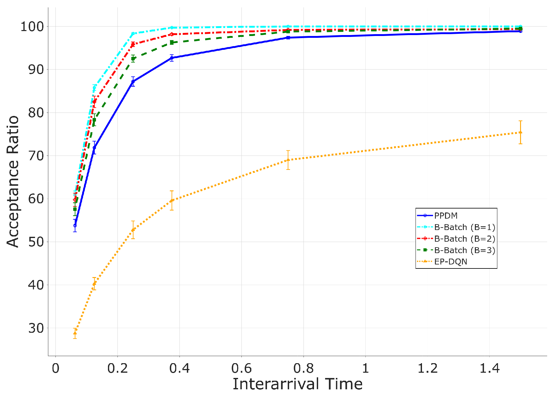
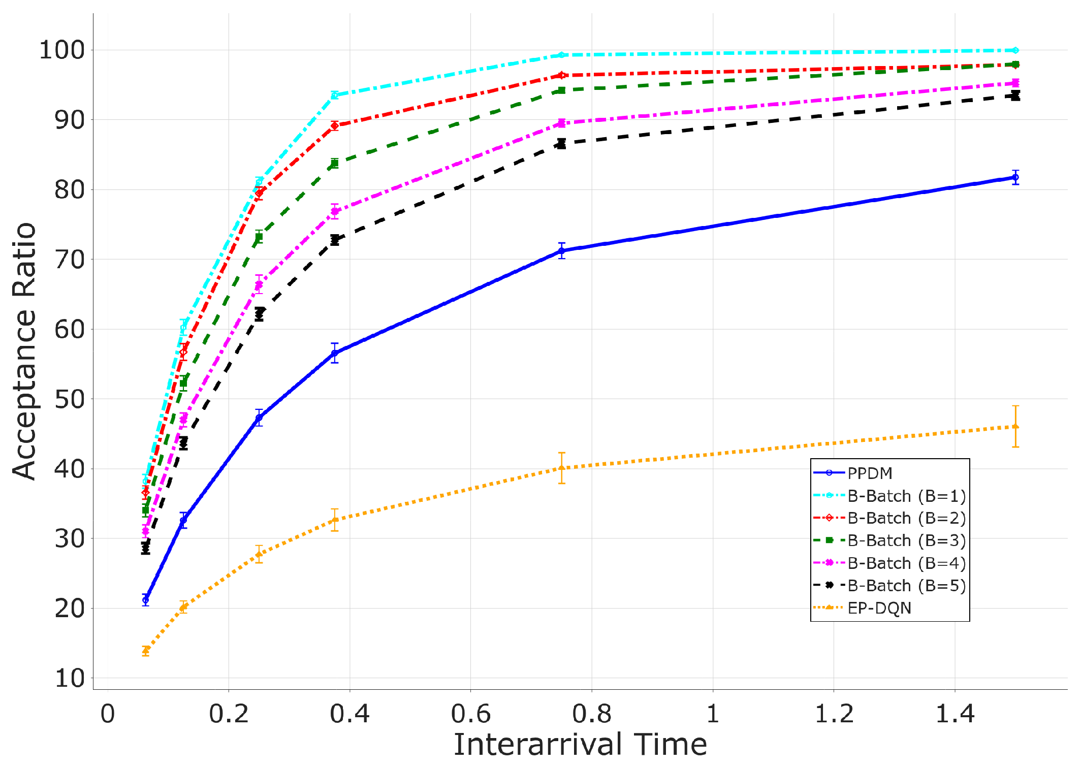
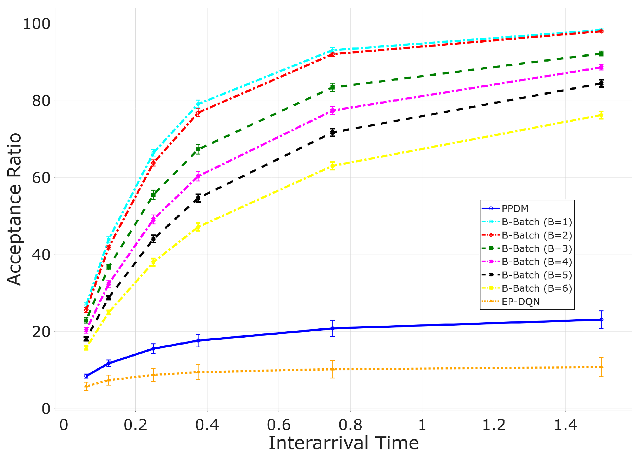
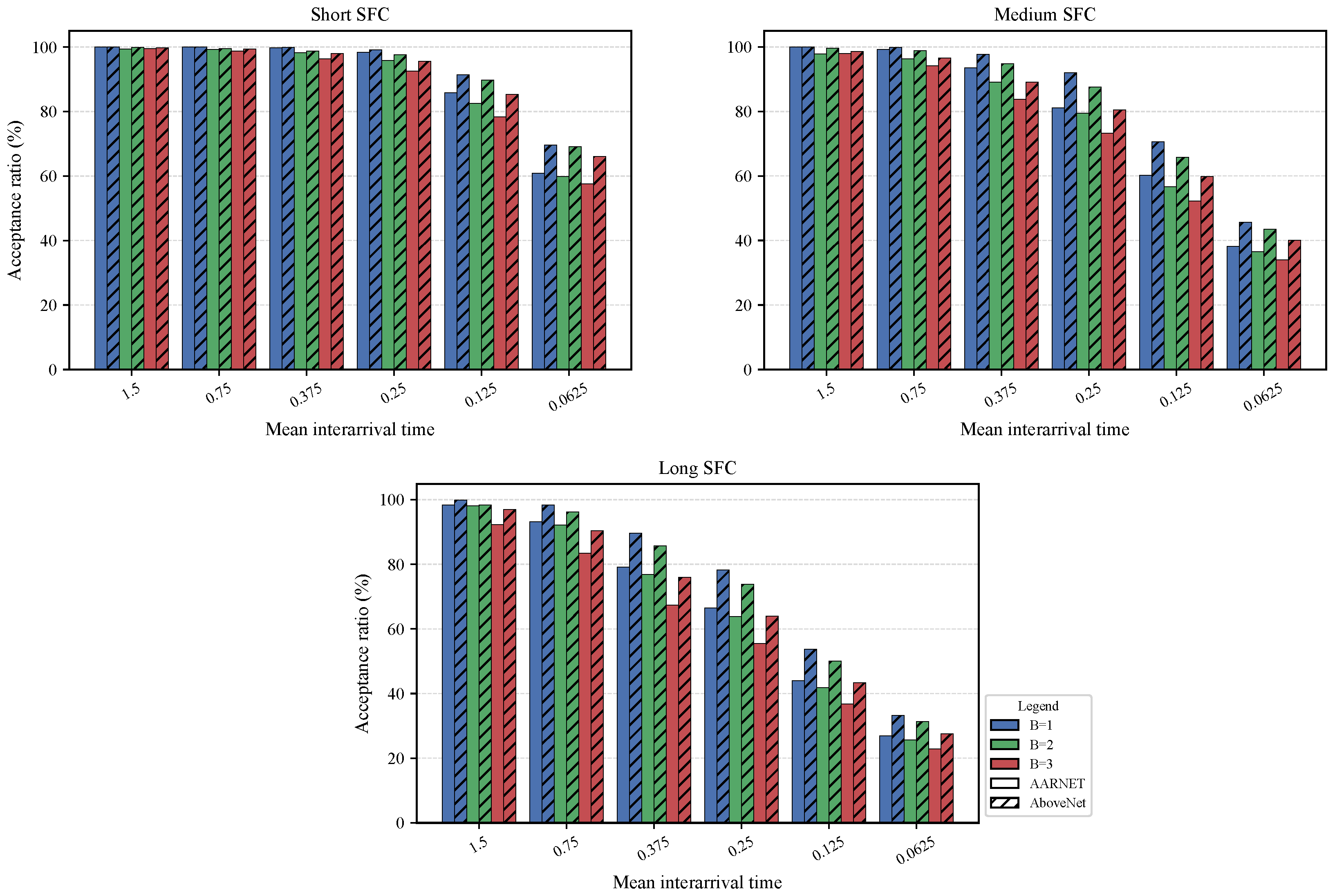
Figure 6, Figure 7 and Figure 8 illustrate the acceptance ratio under varying traffic intensities, with detailed performance for short, medium and long SFCs. In general, the proposed $\mathcal{B}$-Batch mechanisms demonstrate consistently higher acceptance ratios than PPDM and EP-DQN across all traffic regimes. The improvement is particularly clear under medium and heavy traffic conditions, where resource availability becomes more limited.

Figure 6 shows that, for short SFCs, the $\mathcal{B}$-Batch mechanisms outperform PPDM and EP-DQN throughout the full range of interarrival times. In light traffic, $\mathcal{B}=1$ achieves near-perfect acceptance, while PPDM and EP-DQN remain lower. As traffic load increases, the performance gap becomes more pronounced. For example, under the heaviest traffic condition ($T=0.0625$), PPDM and EP-DQN decrease to $53.77\%$ and $28.76\%$, respectively, while variants $\mathcal{B}$-Batch maintain higher acceptance ratios. Among the variants of the $\mathcal{B}$-Batch mechanism, smaller batch sizes provide better acceptance, with $\mathcal{B}=1$ achieving the highest acceptance ratio.

Figure 7 shows that the advantage of the $\mathcal{B}$-Batch mechanisms becomes more evident for medium SFCs. As traffic intensity increases, PPDM and EP-DQN experience a sharp decrease in the acceptance ratio. In contrast, the $\mathcal{B}$-Batch mechanisms maintain higher acceptance ratios across all traffic levels. Under the heaviest traffic condition, $\mathcal{B}=1$ achieves the highest acceptance ratio among the variants of the $\mathcal{B}$-Batch mechanism, followed by $\mathcal{B}=2$ and $\mathcal{B}=3$. This result indicates that increasing batch size gradually reduces acceptance performance because more VNFs are evaluated simultaneously during SIRM construction.

Figure 8 presents the acceptance ratio for long SFCs, where the embedding task is the most challenging. PPDM and EP-DQN show consistently low acceptance ratios across the traffic range, reflecting the difficulty of sustaining feasible embeddings for long SFCs under limited substrate resources. In contrast, the $\mathcal{B}$-Batch mechanisms achieve substantial improvements, especially under light and moderate traffic conditions. However, the acceptance ratio still decreases as the batch size increases, showing that smaller batch sizes are more effective in preserving feasible deployment options for long SFCs.

To better understand the observed trends, we further analyze the underlying causes of these results. We begin with the short SFC scenario, where the impact of batch size is most clearly observed. For short SFC, small batch sizes ($\mathcal{B}=1$) consistently achieve higher acceptance ratios, whereas PPDM, which constructs the SIRM over the entire SFC, exhibits lower acceptance in all traffic conditions. As traffic intensity increases, more SFCs are active simultaneously, reducing available substrate resources. Consequently, more substrate nodes are considered infeasible during SIRM construction, leading to a higher occurrence of ambiguous states. This reduces the number of feasible deployment options and the acceptance ratio.

EP-DQN exhibits an even lower acceptance ratio than PPDM across all SFC lengths. During state construction, all substrate nodes perform virtual occupation simultaneously, artificially locking network capacity. As a result, resources appear to be depleted earlier than in the actual system, creating a mismatch between the true availability of resources and the observed state. This mismatch increases the likelihood of ambiguous states, further reducing the number of feasible deployment options and lowering the acceptance ratio.

For medium and long SFCs, the difference in the acceptance ratio between small batches, large batches, PPDM, and EP-DQN becomes more pronounced. This is because SFCs with a larger number of VNFs require more simultaneous feasibility evaluations, which increases virtual resource occupation within a single SFC. As a result, ambiguous states occur more frequently, amplifying the negative impact of inaccurate state representation in EP-DQN and further widening the performance gap compared to the batch-based approach.

In general, the results indicate that smaller batch sizes consistently achieve higher acceptance ratios across all SFC lengths and traffic conditions, with the sequential deployment strategy ($\mathcal{B}=1$) providing the most robust embedding performance. This process can be explained by the level of ambiguity in the SIRM, which is fundamentally governed by virtual resource occupation during state construction. With increasing traffic intensity and longer SFC lengths, multiple VNFs must be evaluated simultaneously, leading to significant virtual reservation of substrate resources. This process artificially reduces the perceived availability of resources, causing many candidate substrate nodes to be incorrectly classified as infeasible. As a result, the SIRM becomes increasingly dominated by ambiguous states, where few feasible deployment options are identified. This effect is particularly severe in PPDM, which constructs the SIRM over the entire SFC and thereby amplifies virtual occupation. Although EP-DQN uses substrate node information rather than SIRM, its decision quality can still degrade under heavy traffic because resource depletion reduces the availability of feasible substrate nodes. In contrast, the proposed $\mathcal{B}$-Batch mechanism mitigates this issue by limiting feasibility evaluation to smaller subsets of VNFs. By reducing virtual resource occupation, the resulting SIRM more accurately reflects the true substrate state, enabling the DQN agent to make more reliable decisions. Consequently, feasible deployment options are better preserved even in high traffic conditions and large SFC sizes. These findings highlight that controlling SIRM ambiguity, rather than solely improving learning capability, is the key factor for robust multi-domain SFC embedding.

6.1.2. End-to-End Delay Testing

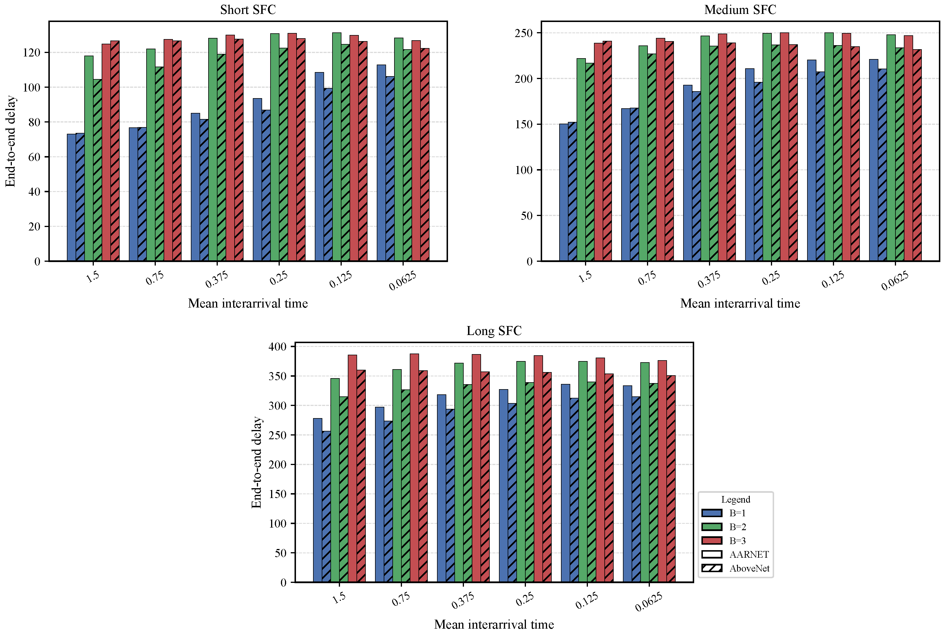
Figure 9 shows the end-to-end delay for short SFCs. PPDM consistently operates in a high-delay region across all traffic intensities, while EP-DQN achieves lower delay than PPDM. In contrast, the proposed $\mathcal{B}$-Batch mechanism with $\mathcal{B}=1$ provides the lowest delay among all mechanisms. For example, under light traffic, $\mathcal{B}=1$ achieves a delay of $73.10$ time units, which is substantially lower than PPDM and EP-DQN. The variants with $\mathcal{B}=2$ and $\mathcal{B}=3$ show intermediate delay performance and remain relatively stable across different traffic intensities. These results indicate that, for short SFCs, the smallest batch size provides the most favorable latency performance, while larger batch sizes result in a more stable but higher-delay operating region.

Figure 10 shows the delay performance for medium SFCs. PPDM again maintains relatively high delay values across all traffic intensities, while EP-DQN provides intermediate delay performance. Among the $\mathcal{B}$-Batch mechanism, $\mathcal{B}=1$ achieves the lowest delay in light traffic. However, its delay increases as the traffic load intensifies and approaches the PPDM baseline under heavy traffic. In contrast, larger batch sizes ($\mathcal{B}\ge 2$) generally produce longer delays, particularly under medium and heavy traffic conditions. For example, at $T=0.25$, the delay increases as the batch size increases, indicating that larger batches can introduce additional routing and/or deployment-induced latency for medium chains.

Figure 11 presents the delay results for long SFCs, where the latency overhead is the highest due to the increased embedding complexity. PPDM produces consistently high delay values under all traffic conditions. The proposed $\mathcal{B}$-Batch mechanism with $\mathcal{B}=1$ reduces the delay relative to PPDM and provides the best latency performance among privacy-preserving mechanisms. However, the delay increases substantially when larger batch sizes are used. Under the heaviest traffic conditions, for example, $\mathcal{B}=2$, $\mathcal{B}=3$, and $\mathcal{B}=4$ result in a longer delay than $\mathcal{B}=1$. EP-DQN achieves a lower delay than PPDM but remains higher than $\mathcal{B}=1$. In general, these results demonstrate that $\mathcal{B}=1$ provides the most favorable latency profile for delay-sensitive operation, while larger batch sizes may increase end-to-end delay, particularly for medium and long SFCs.

To better understand these observations, we analyze the underlying causes of the delay behavior. For short SFC, most scenarios operate under sufficient resource conditions, where the total SFC demand remains within the available substrate capacity. As a result, the top-$\eta$ candidate nodes remain relatively stable in all methods, and the difference in end-to-end delay is small. However, as traffic intensity increases, virtual occupation becomes more significant in larger batch sizes and PPDM, causing many feasibility indicators ${\xi }_{n_j^k}^{v_i^l}$ to be zero. This leads to ambiguous SIRM states, where the DQN agent cannot clearly identify suitable deployment candidates. Consequently, the acceptance ratio decreases, while the average end-to-end delay remains relatively unchanged.

For medium and long SFCs, the impact of virtual occupation becomes more pronounced, as the total virtual resource demand more frequently exceeds the available substrate capacity. In these cases, larger batch sizes and PPDM generate more ambiguous SIRM states during candidate selection. As a result, the DQN agent must select from a frequently changing top-$\eta$ candidate node set. This leads to the selection of different substrate nodes across consecutive VNFs, resulting in less compact service paths and increased end-to-end delay. In contrast, smaller batch sizes maintain a more stable candidate node set over a wider range of traffic conditions, enabling more consistent deployment decisions and more compact service paths.

EP-DQN exhibits lower end-to-end delay than PPDM, but a higher delay than the $\mathcal{B}$-Batch mechanism approach with $\mathcal{B}=1$. This behavior arises because EP-DQN performs a simultaneous virtual reservation for multiple VNFs during state construction. As a result, some substrate nodes appear to exhaust their available resources earlier than in the actual system and are therefore selected less frequently by the DQN agent. This leads to suboptimal and less consistent node selection across VNFs, producing less compact service paths.

In contrast, the $\mathcal{B}=1$ strategy more accurately reflects the true resource condition of the substrate nodes by limiting the virtual occupation. Consequently, the SIRM state remains more consistent across VNFs within the same SFC, allowing the DQN agent to repeatedly select the same or nearby substrate nodes. This results in more compact service paths and lower end-to-end delays. This effect becomes more pronounced for medium and long SFCs.

In general, the end-to-end delay results shown in Figure 9, Figure 10 and Figure 11 indicate that smaller batch sizes consistently achieve a lower and more stable delay across different SFC lengths and traffic intensities. In particular, the $\mathcal{B}$-Batch mechanism strategy with $\mathcal{B}=1$ provides the most compact deployment behavior. This is because smaller batches introduce minimal virtual occupation during the candidate selection stage, allowing the DQN agent to evaluate substrate nodes using more accurate and less constrained resource information. Consequently, the top-$\eta$ candidate node set remains stable across consecutive VNFs, allowing the DQN agent to repeatedly select the same or nearby substrate nodes and construct shorter service paths.

6.1.3. Resource Utilization Testing

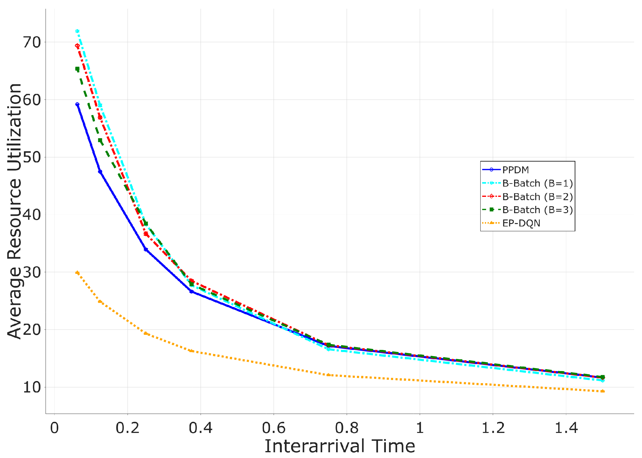
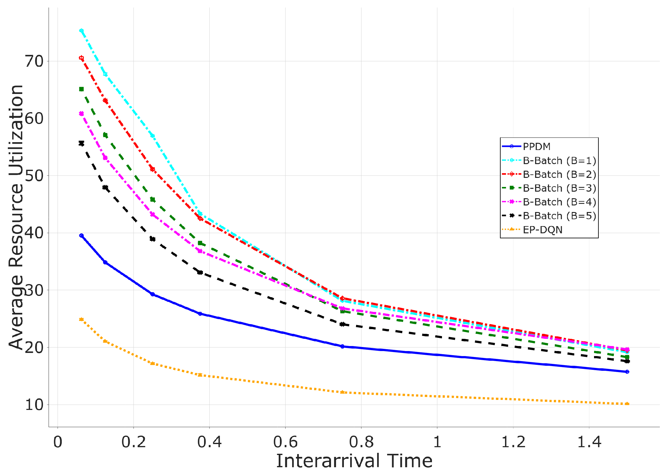
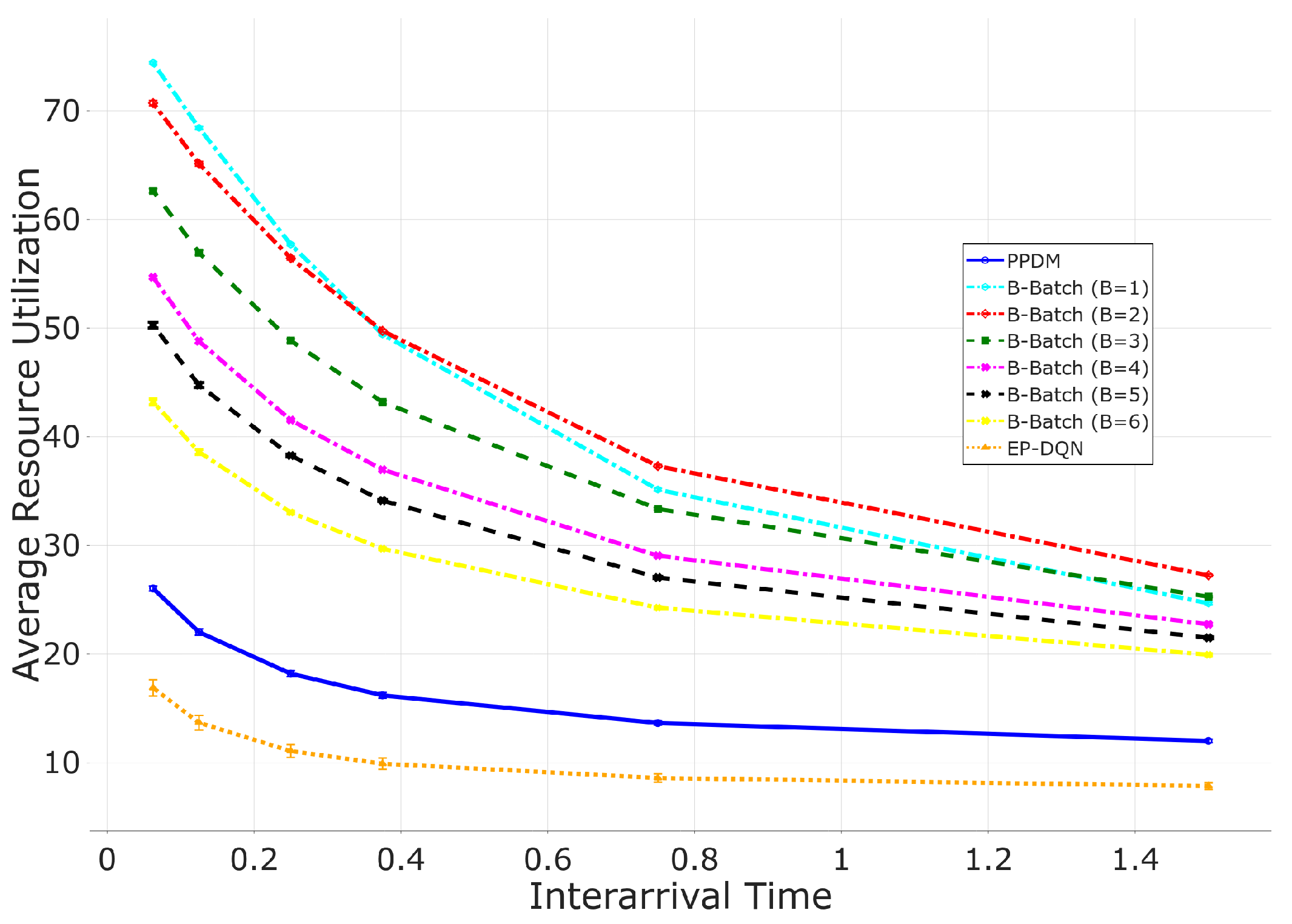
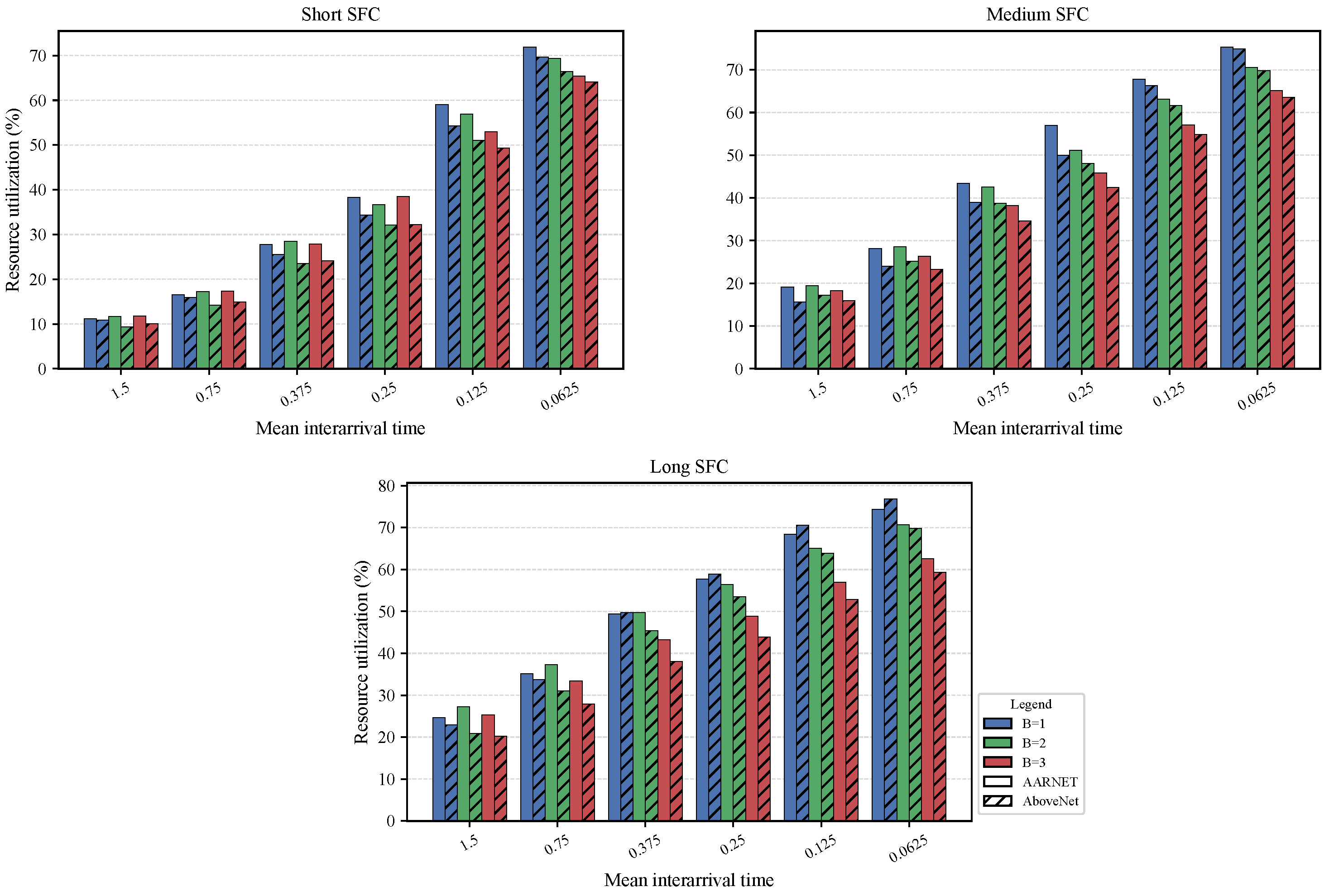
Figure 12, Figure 13 and Figure 14 illustrate the average utilization of substrate resources as a function of the interarrival time for short, medium, and long SFCs. In all scenarios, resource utilization increases as the interarrival time decreases, indicating that heavier traffic leads to higher substrate resource usage. This trend is consistent with the acceptance ratio results, where a larger number of successfully embedded SFCs increases the overall resource consumption.

Figure 12 shows the resource utilization results for short SFCs. Under light and moderate traffic conditions, all mechanisms operate in a low-utilization region because only a limited amount of substrate resources is required to embed short chains. As traffic intensity increases, resource utilization increases for all mechanisms, and the difference among the methods becomes more visible. Under the heaviest traffic conditions, the $\mathcal{B}$-Batch mechanisms achieve higher resource utilization than PPDM and EP-DQN, with $\mathcal{B}=1$ reaching the highest utilization. This result is consistent with the stronger acceptance performance of the proposed batch-based mechanisms under high traffic conditions.

Figure 13 shows the resource utilization behavior for medium SFCs. Compared with the short SFC scenario, the difference among the mechanisms becomes clearer because medium SFCs require more substrate resources for successful embedding. PPDM and EP-DQN show relatively low utilization, reflecting their lower acceptance ratios. In contrast, the $\mathcal{B}$-Batch mechanisms achieve substantially higher utilization, particularly with smaller batch sizes. In heavy traffic, $\mathcal{B}=1$ achieves the highest utilization, followed by larger batches. As $\mathcal{B}$ increases, substrate resource utilization gradually decreases, which is consistent with the reduction in the acceptance ratio caused by a greater virtual occupation during SIRM construction.

Figure 14 presents the utilization results for long SFCs. In this scenario, PPDM and EP-DQN maintain low utilization across the traffic range because only a small number of long SFC requests can be successfully embedded. In contrast, the $\mathcal{B}$-Batch mechanisms substantially increase the usage of substrate resources. Under the heaviest traffic conditions, the smaller batch sizes achieve the highest utilization, while utilization decreases as the batch size increases. This monotonic decline indicates that larger batch sizes introduce a higher virtual occupation, which reduces the number of feasible deployment options and leads to fewer successful embeddings.

To better understand these results, we further analyze the relationship between resource utilization, acceptance ratio, and batch size. For short SFCs, the difference in resource utilization between methods is relatively small under light to moderate traffic conditions, where all mechanisms operate in a low use regime (below 30%). As traffic intensity increases, resource utilization increases for all methods, and the performance gap becomes more visible. As traffic increased, the $\mathcal{B}$-batch mechanisms achieve higher utilization than PPDM, with $\mathcal{B}=1$ reaching the highest values. However, the increase in utilization does not always follow the same trend as the acceptance ratio. In some cases, methods with similar acceptance ratios exhibit different levels of utilization, indicating that resource usage is also influenced by how VNFs are distributed between substrate nodes.

For medium and long SFCs, resource utilization becomes more distinct between methods. As the total resource demand more frequently exceeds the available substrate capacity, the effect of batch size becomes more pronounced. Smaller batch sizes consistently achieve higher utilization, with $\mathcal{B}=1$ reaching the highest values under heavy traffic. In contrast, resource utilization decreases monotonically as the batch size increases, which is consistent with the reduction in the acceptance ratio due to the higher virtual occupation. Both PPDM and EP-DQN show low utilization compared to the proposed system, particularly for long SFCs, where only a small number of requests can be successfully embedded.

However, the relationship between acceptance ratio and resource utilization is not strictly linear. In several cases, particularly for $\mathcal{B}=1$, higher acceptance ratios do not directly translate into proportionally higher utilization. This behavior suggests that the agent tends to repeatedly select a compact subset of highly feasible substrate nodes, leading to embeddings with limited spatial dispersion across the substrate network. As a result, VNFs are concentrated on a small set of nodes rather than being distributed across the entire infrastructure, keeping the overall average utilization relatively lower despite the higher number of accepted requests.

This node-repetition behavior is consistent with the reward structure in Equation (17), where the repetition penalty $r(\rho \mid s_t,a_t)$ remains relatively small compared to the feasibility reward $r(\delta \mid s_t,a_t)$ and therefore provides only a weak incentive to diversify substrate node selections. Consequently, deployment decisions can lead to localized hotspot formation rather than uniformly balanced resource utilization across domains.

Overall, the results indicate that substrate resource utilization increases as traffic intensity increases, which is consistent with the higher number of successfully embedded SFCs. Across all scenarios, smaller batch sizes achieve higher utilization because they introduce a lower virtual occupation, allowing more SFCs to be successfully embedded. In contrast, larger batch sizes and PPDM introduce a higher virtual occupation, which limits the number of accepted requests and results in lower utilization.

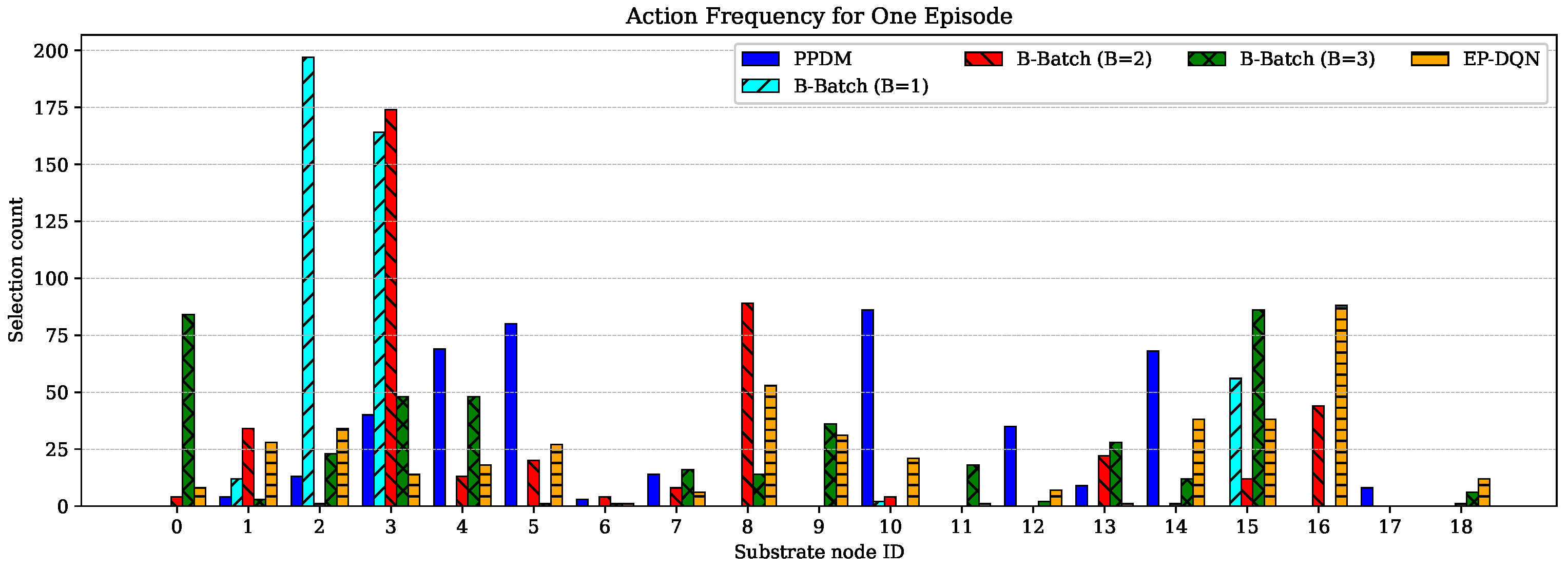
6.2. Node Selection Behavior Analysis

The node selection patterns of the evaluated mechanisms provide additional insight into the operational causes behind the acceptance-ratio, delay, and utilization trends reported above. For the node selection behavior analysis, we capture the substrate node choices from one representative testing episode, where the episode consists of 100 consecutive short SFC requests. This snapshot is used to provide an intuitive visualization of how each mechanism distributes its deployment decisions across substrate nodes under the same traffic realization. In this analysis, we consider the short SFC scenario, evaluated under both normal traffic conditions (interarrival time = 12) and burst traffic conditions (interarrival time = 8), to illustrate how different mechanisms respond to varying traffic intensities.

Figure 15 visualizes the substrate node selection frequency of each mechanism by counting how often each substrate node is selected during the episode. PPDM and EP-DQN exhibit a relatively wider spread of selections across the substrate, indicating that their decisions are not concentrated on a small set of nodes. For PPDM, this behavior is consistent with the virtual occupation effect, which causes the top-$\eta$ candidate substrate nodes to change progressively during the embedding process. In EP-DQN, the effect is even more pronounced, as virtual reservation is applied simultaneously across all candidate substrate nodes, leading to stronger distortion in resource availability. As a result, the policy is frequently forced to switch away from previously feasible substrate nodes toward alternative candidates and increasing dispersion of selected substrate node.

In contrast, the proposed $\mathcal{B}$-Batch mechanism demonstrates a more structured node selection pattern in the evaluated batch settings $\mathcal{B}\in \{1,2,3\}$. When $\mathcal{B}=1$, the selection frequency is noticeably concentrated on a small subset of highly feasible nodes, reflecting stronger reuse of nodes. This behavior aligns with the reward structure in Equation (17), where the feasibility reward $r(\delta \mid s_t,a_t)$ dominates the decision objective, while the repetition penalty $r(\rho \mid s_t,a_t)$ remains comparatively smaller after normalization. Consequently, once a feasible substrate node is identified, the agent is incentivized to repeatedly exploit it, which explains the higher acceptance ratio and the lower delay observed for $\mathcal{B}=1$ in the previous subsection.

For larger batch settings ($\mathcal{B}=2$ and $\mathcal{B}=3$), Figure 15 shows a more distributed selection profile, where deployments are spread over a broader set of substrate nodes compared to $\mathcal{B}=1$. This occurs because resource reservation within each batch increases virtual occupation more rapidly for repeatedly selected nodes, causing top-$\eta$ candidate change more frequently than $\mathcal{B}=1$.

In general, Figure 15 confirms that PPDM and EP-DQN exhibit a higher degree of virtual occupation, resulting in a more dispersed selection of substrate nodes. In contrast, the proposed $\mathcal{B}$-Batch mechanism introduces a lower virtual occupation and produces more consistent deployment patterns. Specifically, smaller batch sizes promote node reuse, while larger batch sizes encourage broader substrate exploration due to increased virtual-occupation-driven diversification.

6.3. Additional Evaluation on the AboveNet Topology

To further evaluate the generality of the proposed $\mathcal{B}$-Batch mechanism, we conduct an additional evaluation using the AboveNet topology. This evaluation examines whether the performance trends observed on AARNET remain consistent under a different substrate network structure. The comparison considers $\mathcal{B}=1$, $\mathcal{B}=2$, and $\mathcal{B}=3$ for short, medium, and long SFC scenarios under different mean interarrival times. The evaluation focuses on three metrics: acceptance ratio, end-to-end delay, and substrate resource utilization. The results are compared with those obtained on AARNET to analyze whether the trade-off between deployment feasibility and orchestration overhead is topology-dependent or remains consistent across different network structures.

6.3.1. Acceptance Ratio Comparison for Different Topologies

Figure 16 compares the acceptance ratio of AARNET and AboveNet for short, medium, and long SFCs under different mean interarrival times. In general, the acceptance-ratio trends of the $\mathcal{B}$-Batch mechanism are consistent across both topologies. In both AARNET and AboveNet, the acceptance ratio decreases as the mean interarrival time becomes shorter and the SFC length becomes longer. This is because heavier traffic and longer SFCs increase resource competition, making it more difficult to find feasible substrate nodes during deployment.

Under light traffic conditions, AARNET and AboveNet show relatively similar acceptance ratios for all evaluated batch sizes. However, under heavier traffic conditions, the difference between the two topologies becomes more noticeable. This difference is mainly due to differences in the availability of substrate nodes and the distribution of resources. AboveNet contains more substrate nodes than AARNET, which provides more candidate locations for VNF deployment. As a result, AboveNet can offer more feasible placement options under high traffic loads, improving the acceptance ratio.

6.3.2. End-to-End Delay Comparison

Figure 17 compares the end-to-end delay of AARNET and AboveNet for short, medium and long SFCs under different mean interarrival times. For short SFCs, the case $\mathcal{B}=1$ in both topologies shows an increasing delay as the mean interarrival time becomes shorter. This indicates that heavier traffic increases resource competition and makes it more difficult to select substrate nodes with low-delay deployment paths. For $\mathcal{B}=2$ and $\mathcal{B}=3$, the delay also increases with heavy traffic, but tends to become more stable starting from $T=0.25$. This stability occurs because ambiguous SIRM states become more frequent at lower interarrival times, limiting the availability of candidate candidates with low delay.

For medium and long SFCs, the delay becomes stable earlier than in short SFCs for each batch size. This is because longer SFCs require more VNF placements and virtual-link mappings, making the end-to-end delay more sensitive to resource availability and deployment decisions. Nevertheless, the overall delay trend remains consistent across AARNET and AboveNet. The difference in absolute delay values between the two topologies is mainly caused by differences in substrate resource availability and network structure, which produce different SIRM states during candidate selection.

6.3.3. Resource Utilization Comparison

Figure 18 compares the utilization of AARNET and AboveNet substrate resources. In both topologies, resource utilization increases as the mean interarrival time becomes shorter. This is because heavier traffic results in more active SFC requests being deployed on the substrate network.

Resource utilization also increases from short to long SFCs because longer SFCs require more VNF placements and consume more substrate resources. Across both topologies, smaller batch sizes generally lead to higher utilization. This occurs because smaller batches reduce virtual occupation during each orchestration round, improve deployment feasibility, and allow more SFC requests to be accepted. In contrast, larger batch sizes can reduce the acceptance ratio under heavy traffic, resulting in lower substrate resource utilization.

6.3.4. Summary of Topology Generality

The resource utilization results further support the acceptance-ratio and delay observations. Overall, the additional evaluation on AboveNet shows that the relative performance trends among different batch sizes remain consistent across both topologies. Smaller batch sizes generally achieve higher acceptance ratios because they reduce virtual occupation during each orchestration round. In addition, a topology with more feasible deployment options can provide lower-delay placements, which helps reduce the end-to-end delay.

These results indicate that the relationship between batch size and deployment feasibility is not specific to the AARNET topology but can also be observed under a different substrate network structure. Therefore, the AboveNet evaluation strengthens the generality of the proposed $\mathcal{B}$-Batch mechanism in different substrate network environments.

6.4. Signaling and Setup-Time Overhead Analysis

To model the setup time of an SFC request in a multi-domain environment, we express the total setup time as the sum of the aggregate MDC-side processing time and the cumulative signaling time across multiple orchestration rounds:

$$\begin{array}{c}\hfill T_{\mathrm{total}}=T_{\mathrm{processing}}+{\displaystyle \sum _{r=1}^R}{T}_{\mathrm{signaling}}\left(q_r\right),\end{array}$$

(20)

where R denotes the number of orchestration rounds required to complete the deployment, and $q_r$ represents the number of VNFs processed in the r-th round. For an SFC consisting of $|V_v^l|$ VNFs and a batch size $\mathcal{B}$, the number of orchestration rounds is defined as $R=\lceil \left|V_v^l\right|/\mathcal{B}\rceil$, and $q_r=\left|{\mathcal{B}}_r\right|$ corresponds to the size of the r-th batch.

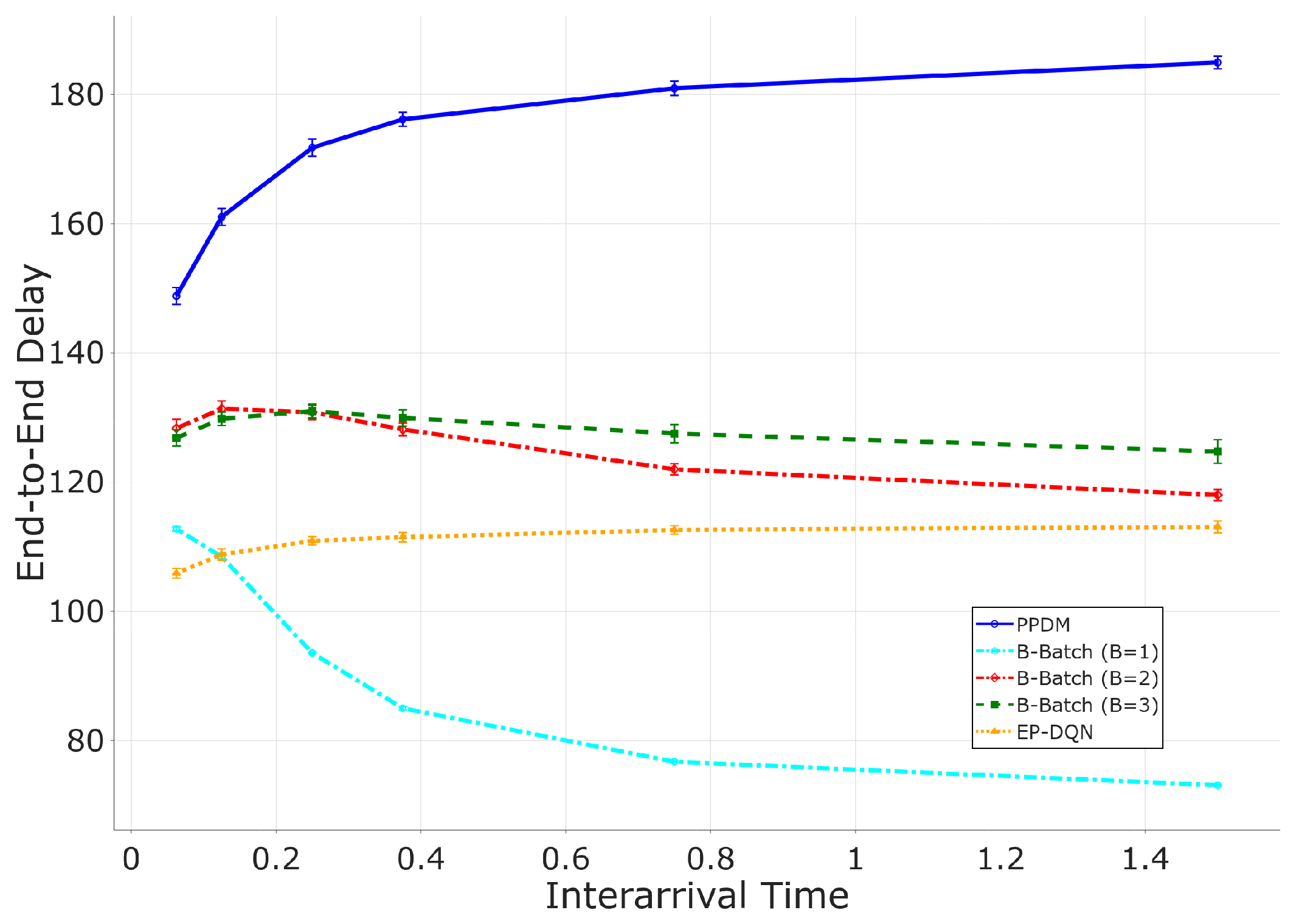
The term $T_{\mathrm{processing}}$ represents the aggregate processing time required to prepare and compute the deployment decision for an SFC request. It includes the initialization time $T_{\mathrm{init}}$, such as coordination between MDC and the LC, state construction, and the decision-making time $T_{\mathrm{deploy}}$, which represents the time required by the LC to deploy the VNFs based on the deployment decisions received from the MDC. In this approximation, these processing components are grouped into a single term because the analysis focuses on the additional signaling overhead introduced by batch-based orchestration.

The term $T_{\mathrm{signaling}}\left(q_r\right)$ denotes the signaling overhead incurred in the r-th orchestration round. This overhead includes the transmission of the current batch from the MDC to the LCs, the batch-level SIRM responses returned by the LCs, and the deployment decision notification sent from the MDC to the selected LCs. Each LC uses its local topology and resource information to evaluate batch feasibility, but only the SIRM response is shared with the MDC.

Figure 19 shows that the impact of $T_{\mathrm{signaling}}$ on the setup delay for long SFCs is scaled by the number of orchestration rounds, i.e., $\lceil \left|V_v^l\right|/\mathcal{B}\rceil$. Therefore, smaller batch sizes lead to higher setup-time overhead because they require more MDC–LC signaling rounds. When $T_{\mathrm{signaling}}$ is relatively small compared to $T_{\mathrm{proc}}$ (e.g., $T_{\mathrm{signaling}}/T_{\mathrm{proc}}=0.5$), the setup-time penalty introduced by smaller batches remains limited, making fine-grained batching acceptable. However, when communication between the MDC and the LCs is costly (e.g., $T_{\mathrm{signaling}}/T_{\mathrm{proc}}=2$), the setup-time penalty increases rapidly as the number of orchestration rounds grows. In such cases, larger batch sizes become more effective in reducing setup-time overhead. Therefore, the batch size $\mathcal{B}$ should be configured according to service requirements, network conditions, and SLAs, reflecting the trade-off between the setup-time overhead and the feasibility of deployment.

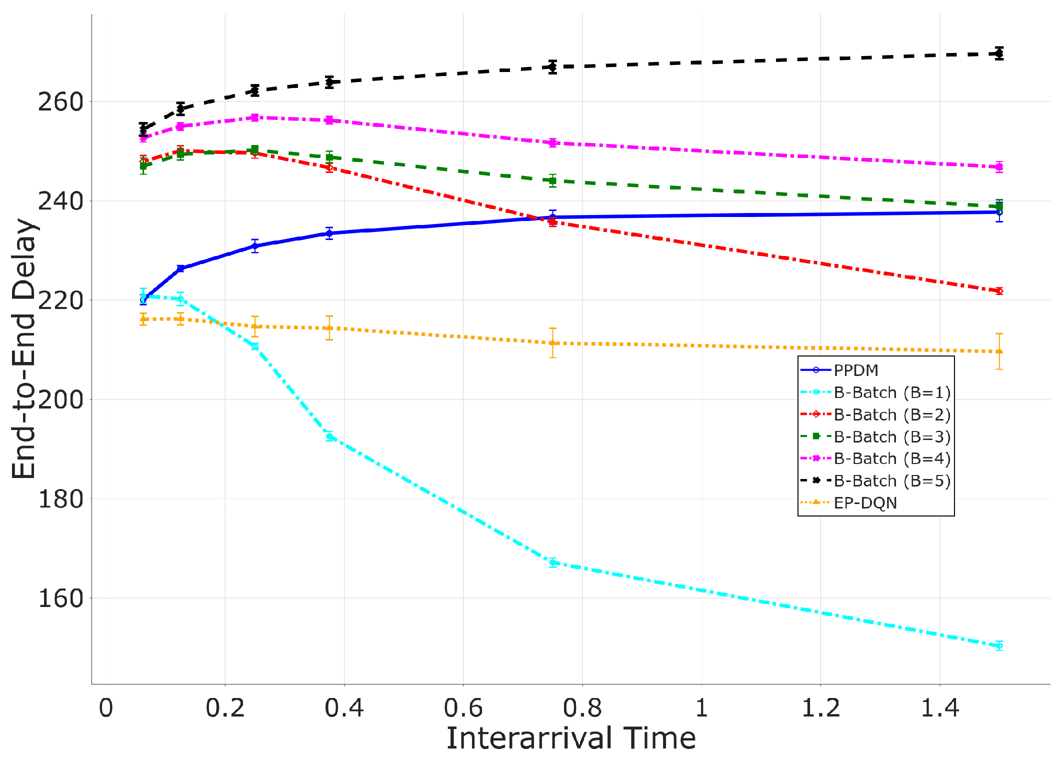
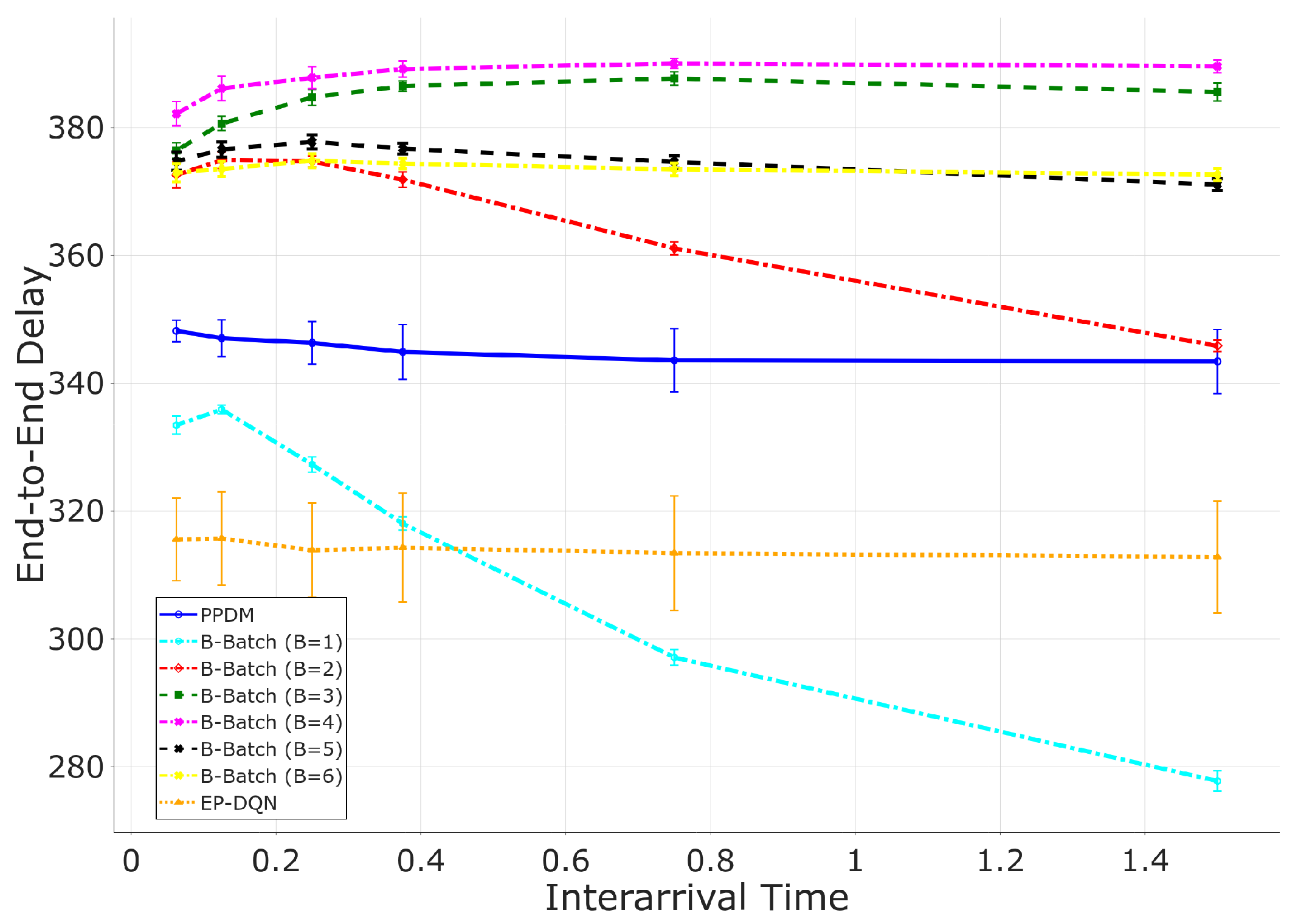
To evaluate this trade-off more directly,

Table 8. Comparison of batch-size trade-offs among different deployment mechanisms.

Deployment Mechanism	Control-ExchangeRounds	Setup-TimeOverhead	Acceptance RatioTendency	End-to-End DelayTendency
$\mathcal{B}=1$	Very High	Very High	Very High	Very Low
$\mathcal{B}=2$	High	High	High	Low
$\mathcal{B}=3$	Moderate	Moderate	Moderate	Moderate
$\mathcal{B}>3$	Low	Low	Low–Moderate	Very High
PPDM	Very Low	Low	Low	High
EP-DQN	Very Low	Low	Very Low	Moderate

summarizes the relationship among deployment granularity, control-exchange rounds, setup-time overhead, and deployment performance tendency. The signaling overhead is reflected in the setup-time model in Equation (20), where the signaling component is accumulated over multiple orchestration rounds. Therefore, the number of control-exchange rounds directly affects the setup-time overhead.

When $\mathcal{B}=1$, each round of orchestration processes only one VNF. This setting minimizes virtual occupation in each round, which can improve the feasibility of deployment and reduce end-to-end delay. However, it requires $R=|V_v^l|$ orchestration rounds, resulting in the highest setup-time overhead.

As $\mathcal{B}$ increases from 2 to values greater than 3, the number of control-exchange rounds and setup-time overhead decreases. However, larger batches also increase the number of VNFs evaluated within the same orchestration round, which may increase virtual occupation and degrade deployment feasibility. Therefore, $\mathcal{B}$ acts as a deployment granularity parameter that balances deployment feasibility, setup-time overhead, and signaling cost.

PPDM represents the full-chain deployment setting, where the whole SFC is evaluated in a single orchestration round. This setting requires only one control-exchange round and therefore has low setup-time overhead. However, because all VNFs are evaluated simultaneously, PPDM suffers from higher virtual occupation, which can reduce the acceptance ratio and increase the end-to-end delay.

EP-DQN has low control-exchange and setup-time overhead because it does not rely on repeated substrate-information exchanges during batch-level deployment. However, its acceptance ratio is very low in our experiments. This occurs because EP-DQN performs virtual occupation over all candidate substrate nodes during state construction, which increases the number of ambiguous states and reduces the feasibility of deployment.

7. Conclusions

This paper investigated privacy-preserving multi-domain SFC deployment in NFV-enabled infrastructures, where infrastructure domains are unwilling to disclose internal topology and resource states to a centralized orchestrator. To preserve privacy, we adopted the SIRM abstraction introduced in PPDM, which restricts inter-domain information exchange to binary feasibility indicators ${\xi }_{n_j^k}^{v_i^l}\in \{0,1\}$. Although this abstraction provides strong privacy isolation, PPDM constructs feasibility information for an entire SFC in a single orchestration round. As a result, virtual occupation can become long-lived and cumulative in the top-$\eta$ candidate set, especially under dense traffic. This condition can distort the SIRM state, reduce the availability of feasible deployment options, and lead to a lower acceptance ratio or unfavorable delay behavior.

To address this limitation, we proposed a $\mathcal{B}$-Batch mechanism that partitions each SFC into fixed-size VNF batches and constructs feasibility information at the batch level. By limiting virtual occupation to the VNFs within the current batch, the proposed mechanism reduces both the magnitude and duration of temporary resource reservation. At the same time, it remains compatible with the SIRM-based privacy model and the hierarchical multi-domain control architecture. A DQN agent was trained to select substrate nodes using only batch-level SIRM information, ensuring that no additional domain-internal topology or resource details are exposed during learning or deployment.

The proposed mechanism remains privacy-preserving because the MDC does not receive actual substrate resource information, internal topology, link states, or routing paths from each domain. Instead, each LC only returns binary SIRM feasibility indicators for the requested batch. However, compared to PPDM, repeated batch-level SIRM exchanges may expose more temporal feasibility patterns over time. For example, repeated binary responses may allow the MDC to observe whether a candidate node frequently becomes feasible or infeasible. Thus, the proposed method prevents direct disclosure of sensitive domain information, although the degree of privacy preservation against long-term inference may be weaker than one-round SIRM exchange mechanisms.

The evaluation on multi-domain AARNET and AboveNet topologies showed that the proposed mechanism improves deployment performance compared with the reference SIRM-based mechanisms, particularly PPDM. The results indicate that $\mathcal{B}$-Batch mechanism improves the reliability of the acceptance ratio under heavier traffic by preserving a more valid feasibility state. The additional evaluation on AboveNet further shows that the relative performance trends among different batch sizes remain consistent across both topologies. Smaller batch sizes generally achieve higher acceptance ratios because they reduce virtual occupation during each orchestration round. In addition, a topology with more feasible deployment options can provide lower-delay placements, which helps reduce the end-to-end delay.

The results also show that batch size $\mathcal{B}$ introduces a practical trade-off between acceptance ratio, end-to-end delay, substrate utilization, and setup-time overhead. Smaller batches reduce virtual occupation and improve feasibility accuracy, but require more orchestration rounds and therefore increase setup time. In contrast, larger batches reduce signaling overhead but may increase SIRM ambiguity. These findings show that $\mathcal{B}$ provides a tunable control parameter to balance privacy-preserving feasibility, deployment performance, and orchestration overhead.

Future work will focus on two directions. First, we will improve the adaptability and performance of the learning model deployment. In this direction, we will investigate topology-generalizable learning models, such as graph neural networks or attention-based architectures, to improve adaptability when the number of domains, substrate nodes, or network topology changes. We will also refine the reward formulation in Equation (17) to better align training optimization with testing objectives under high traffic, particularly by strengthening the relationship between feasibility preservation and delay-sensitive deployment decisions within the top-$\eta$ candidate nodes.

Second, we will strengthen the privacy-preserving aspect of the proposed framework through quantitative privacy analysis and mitigation techniques. In this direction, we will define privacy metrics to evaluate information leakage from repeated batch-level SIRM observations, including feasibility-pattern leakage, candidate-node exposure frequency, and resource-availability inference risk. We will then investigate mitigation techniques such as randomized SIRM responses, candidate rotation, and differential-privacy-based feasibility reporting. We will also explore federated learning for multi-domain policy training, enabling domains to collaboratively improve the DRL policy without exchanging raw substrate information or sensitive operational states.

References

1. Wang, C.X.; You, X.; Gao, X.; Zhu, X.; Li, Z.; Zhang, C.; Wang, H.; Huang, Y.; Chen, Y.; Haas, H.; et al. On the Road to 6G: Visions, Requirements, Key Technologies, and Testbeds. IEEE Commun. Surv. Tutor. 2023, 25, 905–974. [Google Scholar] [CrossRef]
2. Attaoui, W.; Sabir, E.; Elbiaze, H.; Guizani, M. VNF and CNF Placement in 5G: Recent Advances and Future Trends. IEEE Trans. Netw. Serv. Manag. 2023, 20, 4698–4733. [Google Scholar] [CrossRef]
3. Fischer, A.; Botero, J.F.; Beck, M.T.; de Meer, H.; Hesselbach, X. Virtual Network Embedding: A Survey. IEEE Commun. Surv. Tutor. 2013, 15, 1888–1906. [Google Scholar] [CrossRef]
4. Yan, Z.; Ge, J.; Wu, Y.; Li, L.; Li, T. Automatic Virtual Network Embedding: A Deep Reinforcement Learning Approach With Graph Convolutional Networks. IEEE J. Sel. Areas Commun. 2020, 38, 1040–1057. [Google Scholar] [CrossRef]
5. Zheng, D.; Shen, G.; Li, Y.; Cao, X.; Mukherjee, B. Service Function Chaining and Embedding With Heterogeneous Faults Tolerance in Edge Networks. IEEE Trans. Netw. Serv. Manag. 2023, 20, 2157–2171. [Google Scholar] [CrossRef]
6. Nguyen, T.N.; Le, T.V.; Nguyen, M.V.; Nguyen, H.N.; Vu, S. Optimizing Resource Allocation and VNF Embedding in RAN Slicing. IEEE Trans. Netw. Serv. Manag. 2024, 21, 2187–2199. [Google Scholar] [CrossRef]
7. Lu, M.; Gu, Y.; Xie, D. A Dynamic and Collaborative Multi-Layer Virtual Network Embedding Algorithm in SDN Based on Reinforcement Learning. IEEE Trans. Netw. Serv. Manag. 2020, 17, 2305–2317. [Google Scholar] [CrossRef]
8. Xiao, Y.; Ye, Z.; Wu, M.; Li, H.; Xiao, M.; Alouini, M.S.; Al-Hourani, A.; Cioni, S. Space-Air-Ground Integrated Wireless Networks for 6G: Basics, Key Technologies, and Future Trends. IEEE J. Sel. Areas Commun. 2024, 42, 3327–3354. [Google Scholar] [CrossRef]
9. Houidi, I.; Louati, W.; Ben Ameur, W.; Zeghlache, D. Virtual network provisioning across multiple substrate networks. Comput. Netw. 2011, 55, 1011–1023. [Google Scholar] [CrossRef]
10. Dietrich, D.; Rizk, A.; Papadimitriou, P. Multi-domain virtual network embedding with limited information disclosure. In Proceedings of the 2013 IFIP Networking Conference, New York, NY, USA, 22–24 May 2013; pp. 1–9. [Google Scholar]
11. Cai, J.; Zhou, Z.; Huang, Z.; Dai, W.; Yu, F.R. Privacy-Preserving Deployment Mechanism for Service Function Chains Across Multiple Domains. IEEE Trans. Netw. Serv. Manag. 2024, 21, 1241–1254. [Google Scholar] [CrossRef]
12. Chowdhury, M.; Rahman, M.R.; Boutaba, R. ViNEYard: Virtual Network Embedding Algorithms With Coordinated Node and Link Mapping. IEEE/ACM Trans. Netw. 2012, 20, 206–219. [Google Scholar] [CrossRef]
13. Wang, S.; Bi, J.; Wu, J.; Vasilakos, A.V.; Fan, Q. VNE-TD: A Virtual Network Embedding Algorithm Based on Temporal-Difference Learning. Comp. Netw. 2019, 161, 251–263. [Google Scholar] [CrossRef]
14. Ma, S.; Yao, H.; Mai, T.; Yang, J.; He, W.; Xue, K.; Guizani, M. Graph Convolutional Network Aided Virtual Network Embedding for Internet of Thing. IEEE Trans. Netw. Sci. Eng. 2023, 10, 265–278. [Google Scholar] [CrossRef]
15. Zhang, P.; Luo, Z.; Kumar, N.; Guizani, M.; Zhang, H.; Wang, J. CE-VNE: Constraint escalation virtual network embedding algorithm assisted by graph convolutional networks. J. Netw. Comput. Appl. 2024, 221, 103736. [Google Scholar] [CrossRef]
16. Xiao, X. DVNE-DRL: Dynamic Virtual Network Embedding Algorithm Based on Deep Reinforcement Learning. Sci. Rep. 2023, 13, 19789. [Google Scholar] [CrossRef]
17. Wang, T.; Fan, Q.; Li, X.; Zhang, X.; Xiong, Q.; Fu, S.; Gao, M. DRL-SFCP: Adaptive Service Function Chains Placement with Deep Reinforcement Learning. In Proceedings of the IEEE ICC 2021, Montreal, QC, Canada, 14–23 June 2021. [Google Scholar]
18. Wang, T.; Shen, L.; Fan, Q.; Xu, T.; Liu, T.; Xiong, H. Joint Admission Control and Resource Allocation of Virtual Network Embedding via Hierarchical Deep Reinforcement Learning. IEEE Transac. Serv. Comput. 2023, 17, 1001–1015. [Google Scholar] [CrossRef]
19. Tian, A.; Feng, B.; Huang, Y.; Zhou, H.; Yu, S.; Zhang, H. DRL-Based Two-Stage SFC Deployment Approach under Latency Constraints. In Proceedings of the IEEE INFOCOM Workshops 2024, Vancouver, BC, Canada, 20 May 2024. [Google Scholar]
20. Shah, H.A.; Zhao, L. Multiagent Deep-Reinforcement-Learning-Based Virtual Resource Allocation Through NFV in IoT. IEEE Internet Things J. 2021, 8, 3410–3424. [Google Scholar] [CrossRef]
21. Dietrich, D.; Rizk, A.; Papadimitriou, P. Multi-Provider Virtual Network Embedding With Limited Information Disclosure. IEEE Trans. Netw. Serv. Manag. 2015, 12, 188–201. [Google Scholar] [CrossRef]
22. Toumi, N.; Bagaa, M.; Ksentini, A. On Using Deep Reinforcement Learning for Multi-Domain SFC Placement. 2021 IEEE Global Communications Conference (GLOBECOM), Madrid, Spain, 07–11 December 2021. [Google Scholar]
23. Zhang, C.; Wang, X.; Dong, A.; Zhao, Y.; Li, F.; Huang, M. The Intelligent Multi-Domain Service Function Chain Deployment: Architecture, Challenges and Solutions. Int. J. Commun. Syst. 2021, 34, e4665. [Google Scholar] [CrossRef]
24. Yu, H.; Wen, T.; Di, H.; Anand, V.; Li, L. Cost efficient virtual network mapping across multiple domains with joint intra-domain and inter- domain mapping. Opt. Switch. Netw. 2014, 14, 233–240. [Google Scholar] [CrossRef]
25. Quang, P.T.A.; Bradai, A.; Singh, K.D.; Hadjadj-Aoul, Y. Multi-domain non-cooperative VNF-FG embedding: A deep reinforcement learning approach. In Proceedings of the IEEE INFOCOM Workshops, Paris, France, 29 April–2 May 2019; pp. 1–26. [Google Scholar] [CrossRef]
26. Castañeda Cisneros, J.; Pomares Hernández, S.E.; Pérez Sansalvador, J.C.; Rodríguez Henríquez, L.M.; Yangui, S.; Drira, K. Coordination-Free Multi-Domain NFV Orchestration for Consistent VNF Forwarding Graph Reconfiguration. IEEE Trans. Netw. Serv. Manag. 2022, 19, 5133–5151. [Google Scholar] [CrossRef]
27. Lin, R.; Yu, S.; Luo, S.; Zhang, X.; Wang, J.; Zukerman, M. Column Generation Based Service Function Chaining Embedding in Multi-Domain Networks. IEEE Trans. Cloud Comput. 2023, 11, 185–199. [Google Scholar] [CrossRef]
28. Zhang, P.; Chen, N.; Li, S.; Choo, K.R.; Jiang, C.; Wu, S. Multi-Domain Virtual Network Embedding Algorithm Based on Horizontal Federated Learning. IEEE Trans. Inf. Forensics Secur. 2023, 18, 3363–3378. [Google Scholar] [CrossRef]
29. Andreoletti, D.; Velichkova, T.; Verticale, G.; Tornatore, M.; Giordano, S. A Privacy-Preserving Reinforcement Learning Algorithm for Multi-Domain Virtual Network Embedding. IEEE Trans. Netw. Serv. Manag. 2020, 17, 2291–2304. [Google Scholar] [CrossRef]
30. Toumi, N.; Bagaa, M.; Ksentini, A. Hierarchical Multi-Agent Deep Reinforcement Learning for SFC Placement on Multiple Domains. In Proceedings of the 2021 IEEE 46th Conference on Local Computer Networks (LCN), Edmonton, AB, Canada, 4–7 October 2021; pp. 299–304. [Google Scholar] [CrossRef]
31. Zhang, P.; Wang, C.; Kumar, N.; Liu, L. Space-Air-Ground Integrated Multi-Domain Network Resource Orchestration Based on Virtual Network Architecture: A DRL Method. IEEE Trans. Intell. Transp. Syst. 2022, 23, 2798–2808. [Google Scholar] [CrossRef]
32. Slim, L.; Bannour, F. Hierarchical Multi-Agent Deep Reinforcement Learning with an Attention-based Graph Matching Approach for Multi-Domain VNF-FG Embedding. In Proceedings of the GLOBECOM 2023–2023 IEEE Global Communications Conference, Kuala Lumpur, Malaysia, 8–12 December 2023; pp. 2105–2110. [Google Scholar] [CrossRef]
33. Zhang, P.; Xu, Z.; Kumar, N.; Wang, J.; Tan, L.; Almogren, A. Generative adversarial imitation learning assisted virtual network embedding algorithm for space-air-ground integrated network. Comput. Commun. 2024, 228, 107936. [Google Scholar] [CrossRef]
34. Irawan, A.I.; Fukushima, Y.; Miura, H.; Yokohira, T. A Sequential VNF Deployment Mechanism for Privacy-Preserving Multi-Domain SFC Deployment. In Proceedings of the 2025 16th International Conference on Information and Communication Technology Convergence (ICTC), Jeju Island, Republic of Korea, 14–17 October 2025; pp. 1609–1614. [Google Scholar] [CrossRef]
35. Dwaraki, A.; Wolf, T. Adaptive service-chain routing for virtual network functions in software-defined networks. In Proceedings of the 2016 workshop on Hot topics in Middleboxes and Network Function Virtualization, New York, NY, USA, 22–26 August 2016; pp. 32–37. [Google Scholar]
Figure 1. Substrate Network Model and SFC Model.
Futureinternet 18 00312 g001
Figure 2. Hierarchical SFC Deployment Architecture.
Futureinternet 18 00312 g002
Figure 3. Timing Diagram of the PPDM SFC Deployment Mechanism.
Futureinternet 18 00312 g003
Figure 4. Timing diagram of The Proposed B -Batch Sequential Deployment Mechanism.
Futureinternet 18 00312 g004
Figure 5. DQN-Based Substrate Node Selection in the B -Batch Sequential Deployment Mechanism.
Futureinternet 18 00312 g005
Figure 6. Acceptance Ratio for Short SFCs.
Futureinternet 18 00312 g006
Figure 7. Acceptance Ratio for Medium SFCs.
Futureinternet 18 00312 g007
Figure 8. Acceptance Ratio for Long SFCs.
Futureinternet 18 00312 g008
Figure 9. End-to-End Delay for Short SFCs.
Futureinternet 18 00312 g009
Figure 10. End-to-End Delay for Medium SFCs.
Futureinternet 18 00312 g010
Figure 11. End-to-End Delay for Long SFCs.
Futureinternet 18 00312 g011
Figure 12. Average Resource Utilization for Short SFCs.
Futureinternet 18 00312 g012
Figure 13. Average Resource Utilization for Medium SFCs.
Futureinternet 18 00312 g013
Figure 14. Average Resource Utilization for Long SFCs.
Futureinternet 18 00312 g014
Figure 15. Substrate Node Selection Frequency Under Short SFC (one testing episode with 100 SFC requests).
Futureinternet 18 00312 g015
Figure 16. Acceptance ratio comparison between AARNET and AboveNet topologies for different batch sizes under short, medium, and long SFC scenarios.
Futureinternet 18 00312 g016
Figure 17. End-to-end delay comparison between AARNET and AboveNet topologies for different batch sizes under short, medium, and long SFC scenarios.
Futureinternet 18 00312 g017
Figure 18. Substrate resource utilization comparison between AARNET and AboveNet topologies for different batch sizes under short, medium, and long SFC scenarios.
Futureinternet 18 00312 g018
Figure 19. Impact of Batch Size on SFC Setup Deployment Time.
Futureinternet 18 00312 g019