
Article

Performance Assessment of DL for Network Intrusion Detection on a Constrained IoT Device

by
Armin Mazinani
*,
Daniele Antonucci
,
Luca Davoli
and
Gianluigi Ferrari
Internet of Things (IoT) Lab, Department of Engineering and Architecture, University of Parma, 43124 Parma, Italy
*
Author to whom correspondence should be addressed.
Future Internet 2026, 18(1), 34; https://doi.org/10.3390/fi18010034
Submission received: 25 November 2025 / Revised: 1 January 2026 / Accepted: 5 January 2026 / Published: 7 January 2026

Abstract

This work investigates the deployment of Deep Learning (DL) models for network intrusion detection on resource-constrained IoT devices, using the public CICIoT2023 dataset. In particular, we consider the following DL models: Long Short-Term Memory (LSTM), Gated Recurrent Unit (GRU), Recurrent Neural Network (RNN), Convolutional Neural Network (CNN), Temporal Convolutional Network (TCN), Multi-Layer Perceptron (MLP). Bayesian optimization is employed to fine-tune the models’ hyperparameters and ensure reliable performance evaluation across both binary (2-class) and multi-class (8-class, 34-class) intrusion detection. Then, the computational complexity of each DL model is analyzed—in terms of the number of Multiply–ACCumulate operations (MACCs), RAM usage, and inference time—through the STMicroelectronics Cube.AI Analyzer tool, with models being deployed on an STM32H7S78-DK board. To assess the practical deployability of the considered DL models, a trade-off score (balancing classification accuracy and computational efficiency) is introduced: according to this score, our experimental results indicate that MLP and TCN outperform the other models. Furthermore, Post-Training Quantization (PTQ) to 8-bit integer precision is applied, allowing the model size to be reduced by more than 90 % with negligible performance degradation. This demonstrates the effectiveness of quantization in optimizing DL models for real-world deployment on resource-constrained IoT devices.

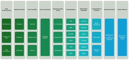
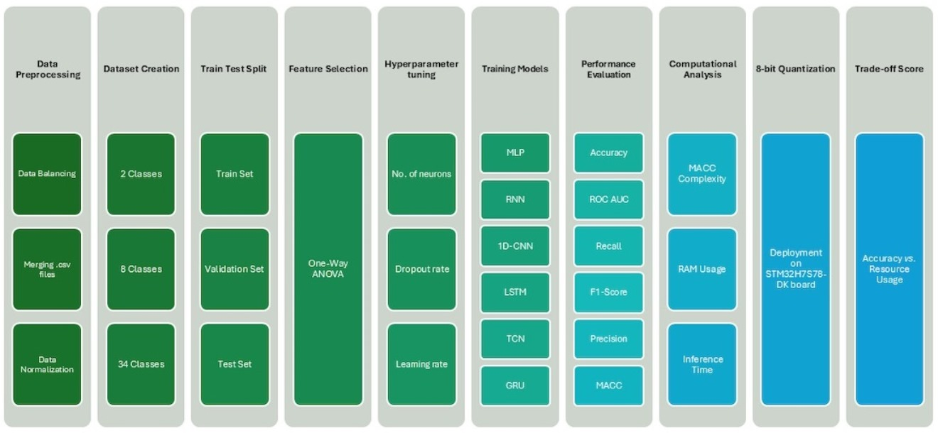
Graphical Abstract

1. Introduction

The Internet of Things (IoT) represents a revolutionary technological paradigm where physical objects—denoted as smart objects and embedded with sensors, software, and connectivity—seamlessly interact with each other and with end-users across heterogeneous communication networks. Therefore, the IoT enables continuous data collection, sharing, and analysis, sustaining innovative concepts such as smart cities, smart agriculture, smart healthcare, and smart homes [1]. In fact, the rapid expansion of IoT is largely driven by advancements in short- (e.g., BLE [2] and Wi-Fi [3]) and long-range wireless networks (e.g., NB-IoT and LoRaWAN [4]), edge computing, Software-Defined Networking (SDN), and sensor innovation [5]. As an example, Cisco foresees that, by 2030, the number of IoT-connected devices will be more than 500 B, owing to the increasing global adoption of IoT technologies across a variety of industries and sectors [6,7].
Nevertheless, this rapid growth also brings significant challenges, in particular with regard to scalability, security, privacy, and data management. As the number of connected devices increases, the detection of unauthorized access and malicious activity within IoT networks becomes an urgent concern [8,9], because the widespread deployment of IoT devices across diverse sectors makes them attractive targets for malicious actors, exposing these devices to a wide range of security threats and vulnerabilities [10].
To this end, security threats on IoT networks vary by network type—literature studies show that approximately 70 % of IoT devices exhibit security vulnerabilities, with an average of 25 faults detected per device [11]—while common vulnerabilities may include the following [12]:
  • Insecure communication: data transmission by IoT devices may occur without adequate encryption, enabling attackers to intercept or manipulate communication [13].
  • Lack of device identity management: the absence of robust Identity Management mechanisms complicates the verification of a device’s authenticity, creating potential security gaps in IoT networks.
  • Insufficient authentication and authorization: many IoT devices lack strong authentication and authorization protocols, allowing unauthorized individuals to access sensitive data or control devices.
To mitigate these risks, Intrusion Detection Systems (IDSs) are recognized as essential components of IoT security infrastructures, monitoring network traffic, detecting potential security threats, and preventing attacks, thereby enhancing the overall security of IoT systems [14]. Therefore, given the growing complexity and scale of IoT networks, the integration of IDSs is crucial to protect against increasingly sophisticated threats targeting connected IoT devices. Simultaneously, applying AI-based models—in particular, Machine Learning (ML) and Deep Learning (DL)—can significantly enhance the performance of IDSs, since these models improve the accuracy of detecting and classifying IoT attacks due to their ability to extract patterns of input data.
In this paper, the performance of different ML and DL models—namely, Simple Recurrent Neural Network (SimpleRNN); Long Short-Term Memory (LSTM); Gated Recurrent Unit (GRU); Multi-Layer Perceptron (MLP); one-dimensional Convolutional Neural Network (1D-CNN)—on a publicly available dataset, denoted as CICIoT2023 [15] and including network traffic traces comprising different attack classes—namely, Denial of Service (DoS); Distributed DoS (DDoS); Spoofing; Web; Brute Force; Recon; Mirai botnet—is detailed and discussed in terms of accuracy and computational complexity. Moreover, Post-Training Quantization (PTQ) is considered for compressing pre-trained models for efficient deployment on constrained IoT devices (e.g., STM32H7S78-DK board [16]).
The main contributions of the paper can be summarized as follows:
  • Resource-constrained IDS design for IoT nodes: We propose an AI-based IDS specifically tailored for deployment on resource-constrained IoT devices, further validated on a STM32H7S78-DK board to address realistic embedded constraints.
  • Comprehensive evaluation on a large-scale, highly imbalanced IoT dataset: The considered IDS is evaluated using the CICIoT2023 dataset, comprising over 46 M network traffic records collected from 105 IoT devices and featuring 34 distinct attack types (including DoS, DDoS, spoofing, brute-force, Mirai botnet attacks, etc.).
  • Systematic handling of class imbalance: A hybrid data balancing strategy, combining random undersampling and random oversampling, is introduced to mitigate the severe imbalance between benign and malicious traffic traces, improving model generalization while avoiding excessive training time and overfitting.
  • Multi-granularity attack classification analysis: Three dataset configurations—namely, binary (2-class), grouped (8-class), and fine-grained (34-class)—are considered, enabling a thorough analysis of the trade-offs between detection accuracy, computational cost, and deployability on a constrained hardware (HW).
  • Feature selection driven by statistical relevance: A one-way ANOVA-based feature ranking is employed to identify and retain the most important features, reducing input dimensionality and computational complexity while preserving essential attack-related correlations.
  • Bayesian optimization for HW-aware hyperparameter tuning: The performance of DL models is enhanced through BO, allowing an efficient exploration of the hyperparameter space while balancing accuracy and computational cost.
  • End-to-end HW-aware evaluation and deployment: Models are evaluated in terms of Multiply–Accumulate operations (MACCs), RAM usage, and inference latency using the STM Cube.AI Analyzer, ensuring practical deployability on a constrained IoT board.
  • Quantization-enabled efficiency enhancement: In order to reduce computational complexity and memory footprint, 8-bit integer quantization of weights and activations is applied, improving inference efficiency while maintaining competitive detection accuracy on the STM32H7S78-DK board.
The remainder of the paper is organized as follows: In Section 2, an overview of related works is given. Section 3 discusses a general representation of an IoT system, together with an overview of common vulnerabilities. Section 4 introduces the chosen dataset, the proposed data analysis techniques, and the considered ML and DL models. Section 5 presents the experimental performance results and the PTQ technique. Finally, in Section 6 we draw our conclusions.

2. Related Works

In order to provide some background on detection and classification of network intrusions and cyber-attacks targeting IoT architectures, in the following we analyze relevant state-of-the-art studies employing ML and DL models and associated evaluation metrics, providing insights into each model’s effectiveness in accurately classifying attacks within the IoT domain. For the sake of clarity and completeness, a comparison between these literature studies presented in the remainder of this section and the model proposed in this paper, along with its main research axes, is shown in Table 1.

2.1. ML/DL Models for IoT NIDS on CICIoT2023

In [17], the performance of several DL models—namely, Deep Neural Networks (DNNs) [25], CNNs, and RNNs—is discussed considering their application to a publicly available dataset (namely, CICIoT2023 [15]). The experimental results show that RNNs return the best performance among all the considered models—with an accuracy of 96.52 % , a precision of 96.25 % , a recall of 96.52 % , and an F1-score of 95.73 % . This reflects the effectiveness of RNNs in detecting both normal and malicious packets, outperforming the other evaluated DL models.
In [15], the authors evaluate five different ML methods—namely, Logistic Regression, Perceptron, AdaBoost, Random Forest (RF), and DNN—across three classification tasks—namely, binary, 8-class, and 34-class classification. Among them, RF demonstrates the highest performance with 83 % recall, 70 % precision, and 71 % F1-score for the 34-class classification, and 91 % recall, 70 % precision, and 71 % F1-score for the 8-class classification. Finally, RF excels in binary classification with 96 % recall, precision, and F1-score, demonstrating its robust performance across varying classification complexities.
In [18], a Federated Learning (FL)-based IDS, aiming at enhancing cybersecurity in IoT networks, is proposed, with FL achieving a 99.0 % accuracy in detecting binary attacks and showcasing the potential of FL in distributed environments where data privacy is essential. Then, class imbalance in the training dataset—a common issue in intrusion detection tasks—is addressed applying the Synthetic Minority Oversampling Technique (SMOTE) [26].
A hybrid model, combining LSTM networks with XGBoost to improve the detection of Mirai botnet attacks, is proposed in [19], benchmarking this approach against alternative models—including DNNs, CNNs, standalone LSTM, and a hybrid RF-LSTM model. Obtained experimental results show that LSTM-XGBoost outperforms the others, in detail achieving a 97.7 % accuracy and 97.4 % precision, recall, and F1-score, thus highlighting its ability to detect complex botnet patterns with high precision and reliability. Additionally, Mirai detection is explored in [20], where a DNN-Light Gradient Boosting Machine (LGBM) hybrid model achieves strong results with accuracy, precision, recall, and F1-score up to 95 % . This performance significantly exceeds that of other models, such as Support Vector Machine (SVM), LGBM, and Stochastic Gradient Descent (SGD), which reach 71 % , 85 % , and 52 % accuracy scores, respectively.
In [21], a CNN-based model is proposed for attack detection, featuring a 4.14  MB model size and a 6 s inference time. This CNN model outperforms alternative models (DNN and LSTM) for binary classification, showing precision, recall, and F1-score equal to 99.43 % , 99.40 % , and 99.41 % , respectively.
A DL-based DDoS detection mechanism is introduced in [22] using a modified GRU (mGRU) model optimized for low computational complexity. In detail, mGRU guarantees a very good performance, achieving 98 % precision, recall, and F1-score. Nevertheless, its efficiency is limited by a high execution time (equal to 10.49  s), indicating its inapplicability in real-time applications.
Finally, binary and multi-class detection of network attacks using classifiers such as SVM, AdaBoost, Decision Tree (DT), and RF are discussed in [23]. In detail, AdaBoost delivers strong results in binary classification, returning a 96 % recall, a 95 % precision, and a 96 % F1-score. However, the larger the number of classes, the more significant the performance degradation: The 8-class classification returns recall, precision, and F1-score drops to 48 % , 56 % , and 48 % , respectively, while the 34-class classification reflects 50 % recall, 58 % precision, and 49 % F1-score.

2.2. TinyML for Intrusion Detection

In [27], the authors investigate the efficiency of TinyML for IoT security by quantizing a two-layer LSTM model (with 64 and 32 units) into a TinyLSTM using TensorFlow Lite on the CICEVSE2024 dataset [28]. As a result, the quantized model achieves an F1-score of up to 99.83 % , while reducing the baseline model size of LSTM by 82 % , the inference time by 76.5 % , and the inference memory by 96.89 % .
Authors in [29] demonstrate the critical trade-offs in deploying TinyML for IoT cybersecurity, showing that while dynamic and static 16-bit floating point quantization techniques effectively balance performance (preserving over 85 % accuracy on the USTC-TFC2016 dataset [30] while halving model sizes and accelerating inference), more aggressive 8-bit integer quantization achieves maximum compression (up to 75 % size reduction) at the cost, however, of severe accuracy degradation. On the other hand, PQT maintains a high detection rate but sacrifices latency and efficiency gains, which are essential for real-time edge deployment.
In [24], a HW-aware intrusion detection framework jointly optimizing accuracy and deployability by enforcing strict flash, RAM, and computing constraints is presented. In detail, the authors combine HW-constrained grid search for tree-based models (LightGBM [31], XGBoost, and RF) with HW-aware neural architecture search for compact 1D-CNNs. The proposed approach is validated on the Edge-IIoTset dataset [32] with an on-device evaluation on an edge gateway–class platform. Notably, all models are evaluated using native inference formats, without applying quantization.
Finally, in [33], a TinyML model for IoT attack detection, combining a lightweight DT and a small NN with a Logistic Regression meta-learner, is deployed on an Arduino Nano 33 BLE Sense. The model achieves exceptional performance on the ToN-IoT dataset [34], returning 99.98 % accuracy, a 99.94 % F1-score, and a near-perfect false positive rate equal to 0.0009 , while operating with ultra-low latency ( 0.12  ms) and power consumption ( 0.01  mW).

3. Vulnerabilities in IoT Architectures

3.1. IoT Layers

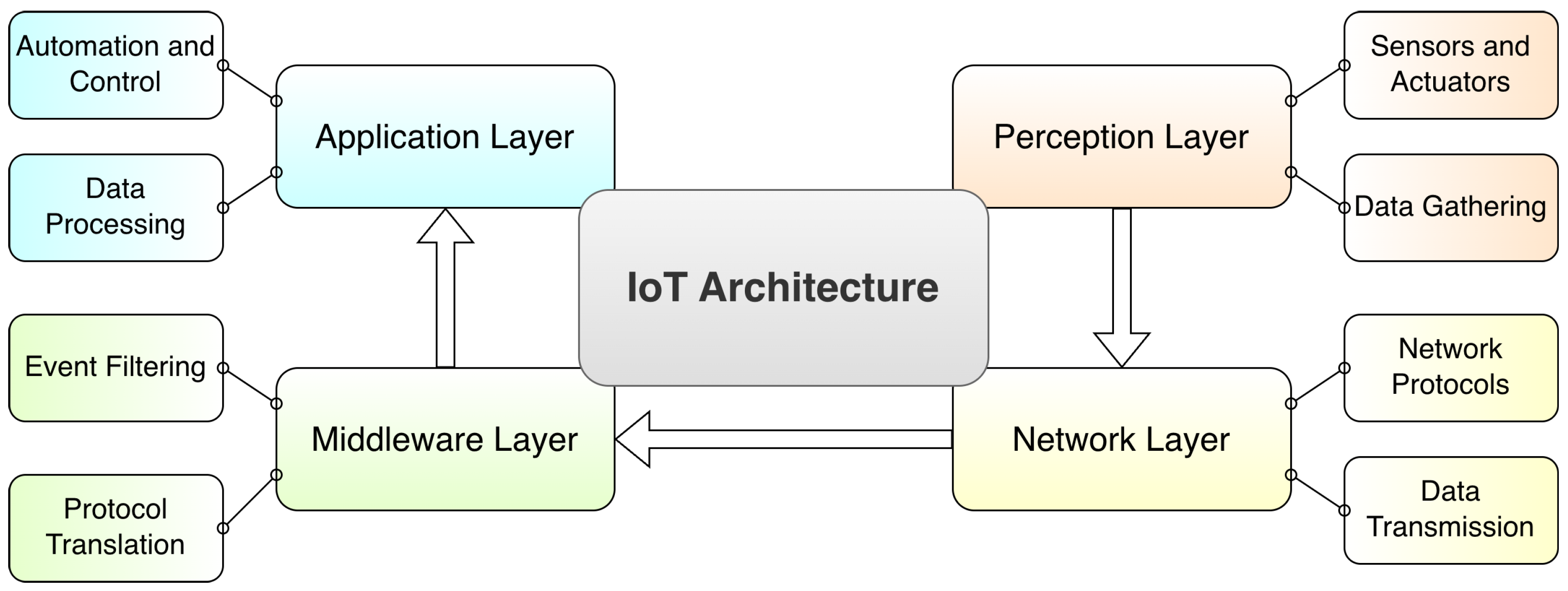
Before analyzing in detail the suitability of the considered AI models in supporting IDS in identifying and classifying IoT network attacks, it is useful to discuss the general architecture of an IoT system, as shown in Figure 1. In detail, an IoT node can be seen as composed of four layers, each featuring the following specific responsibilities in contributing to its seamless integration with other devices.
  • Perception Layer: This layer, also known as sensing layer, corresponds to the lowest layer in an IoT architecture and consists of physical devices—such as sensors, actuators, and smart appliances—directly interacting with the environment to collect and process real-time data.
  • Network Layer Inside an IoT domain, this layer manages the connectivity and the data transmission between IoT devices, gateways, and the higher layers, thus exploiting an ensemble of communication protocols (e.g., Zigbee, BLE, IEEE 802.11 Wi-Fi, LTE/5G cellular, LoRaWAN) to support seamless information transfer across the IoT ecosystem.
  • Middleware Layer: This layer acts as an intermediate layer between network and application layers and provides essential services such as data filtering, aggregation, and protocol translation, thus ensuring interoperability and easing efficient management and deployment of IoT applications.
  • Application Layer: This layer enables specific use cases by delivering services and insights to end-users and additional applications, in detail directly interfacing with the users and providing an ecosystem for the deployment of IoT applications (e.g., smart homes, healthcare, and industrial automation).

3.2. IoT Security Vulnerabilities

In the following, a brief discussion on well-known vulnerabilities of IoT systems is provided from different perspectives.

3.2.1. Active and Passive Attacks

Knowing that cyber-attacks affecting IoT networks can differ with respect to the specific targeted network, the following first classification can focus on the type of actor conducting the attack, namely active or passive:
  • Active attack: it refers to a type of security attack wherein the attacker engages in direct communication with the intended target system or network. This attack involves the deliberate alteration or disruption of a network’s operations through the injection of malicious traffic or the execution of unauthorized commands.
  • Passive attack: it is classified as a security attack wherein the attacker establishes an indirect connection with the target network and observes the communication occurring therein. In this case, an assailant would observe, intercept, or surreptitiously listen to data transfers without making any modifications or exerting any influence over the information, thus primarily aiming to illegally obtain access to sensitive or secret data or information without raising suspicion or detection.
For completeness, in Section 3.2.2, Section 3.2.3, Section 3.2.4 and Section 3.2.5, we delve into attacks specific for each IoT layer detailed in Section 3.1, namely: perception layer, network layer, middleware layer, application layer, respectively. A comprehensive summary of these attacks is given in Table 2.

3.2.2. Attacks to the Perception Layer

The main cyber-challenges the IoT perception layer might suffer for can be summarized as follows:
  • Tampering: This attack aims at creating a direct physical connection with the IoT device and controlling its operational tasks, then involving HW manipulation (e.g., establishing connections with ports or interfaces on the device) or modifications to its settings [35].
  • DoS: This attack foresees an attacker flooding the IoT sensors with an extraordinary volume of traffic or requests, leading to sensor overload, data loss, and service disruption [36].
  • Jamming: This corresponds to a deliberate attack strategy disrupting or obstructing wireless communication signals, thus preventing information transmission [37].
  • Fake node injection: This is one of the most severe attacks for an IoT device, since it features a malicious node to be injected into an IoT network to gain access to such network, then spreading misleading information across the network itself. Consequently, unauthorized nodes will enable an attacker to access the entire network.
  • Sleep deprivation attack: This attack aims at affecting the energy source of (often battery-powered) sensor nodes. In fact, this attack keeps IoT nodes active by altering their sleep cycle—usually employed to minimize their energy consumption—and, consequently, their functionalities, quickly depleting and disrupting the overall IoT network [38].

3.2.3. Attacks to the Network Layer

The main cyber-challenges affecting the network layer can be summarized as follows:
  • Routing attacks: This attack focuses on altering the routes established in the IoT network, thus aiming at transmitting data and messages to malicious intermediary nodes, or interfering with the network’s data transmission process.
  • IP Spoofing: This attack features a malicious node posing as another device or changing the origin IP address inside the packets flowing inside the network itself to tamper with the IoT network and gain unauthorized access.
  • Sybil attack: This attack foresees that the attacker will try to access the network by using a phony identity, in turn also activating fake nodes as normal devices within the network and impairing the network’s operation by creating incorrect and/or large amounts of information [39].
  • Traffic analysis attack: This attack targets to analyze and intercept data packets exchanged intra IoT nodes, as well as between IoT devices and remote entities, in order to extract valuable information.

3.2.4. Attacks to the Middleware Layer

The main cyber-challenges the middleware layer might suffer from can be summarized as follows:
  • Man-in-the-Middle (MITM) attack: This attack foresees the ability of an unauthorized entity to intercept (and potentially manipulate) the communication occurring between IoT devices.
  • Malwares: Threats like viruses, Trojan horses, and malware represent a (sub-)set of tools used by attackers to access (in an unauthorized way) undisclosed and private information, with data theft happening by exploiting executable codes (often developed in machine language).
  • DoS attack: This class of intrusion foresees an attacker overwhelming the IoT network with a heavy amount of requests, thus resulting in the network’s congestion due to excessive traffic. As a result, IoT devices deplete energy and resources, thus preventing the user from accessing his/her data.

3.2.5. Attacks to the Application Layer

Finally, the main cyber-challenges affecting the application layer can be summarized as follows:
  • Cross-Site Scripting (XSS): In this type of attack, the attacker adds harmful scripts to be run (at run-time) into the IoT node’s command-line or Web interfaces, thus compromising its responsiveness as well as the user’s protected information.
  • SQL injection: This attack occurs when the attacker succeeds in manipulating the input parameters used in an SQL query and in executing such malicious SQL queries into the target database.
  • Sniffing attack: This attack involves the ability of the attacker to successfully collect and monitor the data traffic between IoT devices and the services at the application layer, thus handling and controlling them without any authorized permission.

4. Proposed Model

In the following, the proposed IDS, designed to accurately identify and classify IoT attacks by means of AI models suitable for deployment on constrained IoT nodes, is discussed. The proposed models (detailed in Section 4.3) demonstrate their ability to discover intricate interconnections among features in the considered dataset. For completeness, as further outlined in Section 4.1.3, we selectively omit the features that do not significantly contribute to the classification process, thus obtaining an efficient training process execution by diminishing the complexity without sacrificing essential correlations.

4.1. Dataset

In this study, the CICIoT2023 dataset [15] comprising 46 , 686 , 579 records collected from 105 IoT devices, has been identified as the reference dataset. More in detail, the traffic traces include 1 , 098 , 195  benign records and 45 , 588 , 384  malicious records and encompass 33 types of cyber-attacks, including DoS, DDoS, spoofing, brute force, and Mirai Botnet attacks. For completeness, the extracted features and their corresponding descriptions are listed in Table 3.
As detailed in Table 4, three variations in the dataset have been considered in order to conduct a comprehensive evaluation: (i) a 34-class ( C = 34 ) dataset retaining all the attack types; (ii) an 8-class ( C = 8 ) dataset, obtained by grouping together similar classes of attack; and (iii) a binary (2-class, C = 2 ) dataset, obtained by splitting the network attacks into benign and malicious predominant classes. As a first remark, this allows for a thorough analysis of the performance returned by the proposed IDS exploiting different DL models. Then, as a second remark, reducing the number of classes enhances the approach applicability, decreases the training time, and lowers memory and computational requirements.
Looking at the distributions of the considered attack classes detailed in Table 4, it should be highlighted that the majority of the occurrences are related to DoS and DDos attacks, thus leading to an a priori imbalanced dataset. This aspect has to be carefully taken into account when discussing the performance of the AI models embedded in an IDS. Hence, for completeness, the class distributions for 2-, 8-, and 34-class configurations are listed in Table 5, Table 6, and Table 7, respectively.
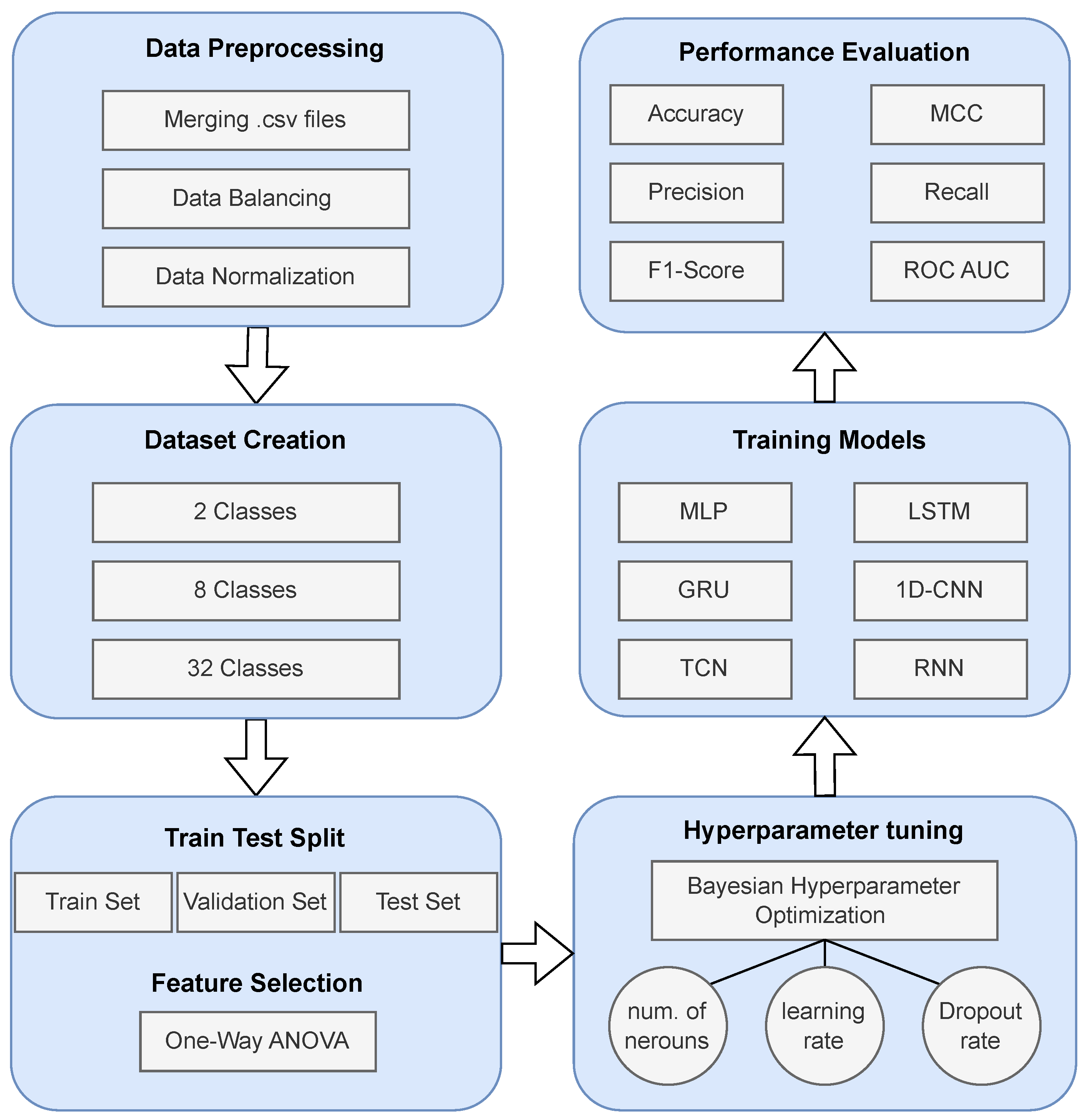
Finally, even for clarity and completeness, the overall approach adopted to refine the dataset—addressing its imbalance and complexity—and to train the chosen AI models is shown in Figure 2. Then, each AI algorithm is subsequently evaluated, exploiting the set of metrics detailed in Section 4.4.

4.1.1. Data Balancing

In order to address the imbalance of the dataset (as mentioned at the beginning of Section 4.1) and mitigate the overfitting effect, the target’s sample size has been defined as based on the data labeled as benign and representing normal network flows. Furthermore, a Random UnderSampler [40] has been applied in order to reduce the majority classes to match the target sample number—equal to 878 , 556 —and to ensure a more balanced class distribution without introducing any bias toward dominant categories. Then, a Random OverSampler [26] has been applied to the minority classes to increase their sample size, thus aligning them with the target. This combined approach enhances the ability of the model to generalize across both benign and malicious instances, thus improving the performance of the IDS while reducing the risk of false positives. Moreover, balancing the dataset before training prevents the model from learning the dominant class distribution, thus ensuring a more comprehensive understanding of all categories. The combined application of these sampling techniques addresses the challenge of oversampling a heavily imbalanced dataset, which may lead to extremely long training times and the risk of generating non-representative samples, possibly causing a degradation in the model’s ability to generalize.

4.1.2. Data Normalization

Since a normalization stage is essential for ensuring all features uniformly contribute to the model (preventing any single variable from dominating the learning process), they are measured on the chosen CICIoT2023 dataset on different scales. Unfortunately, this may negatively affect the models’ performance. Hence, using a scaler is crucial to mitigate the impact of these varying scales, leading to a fair consideration of each feature during model training.
To this end, a PowerTransformer [41], which not only normalizes the features but also stabilizes the variance and makes the data distribution more Gaussian-like, has been employed. This transformation is particularly beneficial, as the model’s convergence speed increases and its overall performance improves, thus allowing more effective learning and generalization. For each anomaly detection configuration (namely, 2, 8, and 34 classes), the dataset was partitioned into three subsets: 60 % for training, 20 % for validation, and 20 % for testing.

4.1.3. Feature Selection

Finally, particular attention has been dedicated to the quality of the dataset. Knowing that quality plays a critical role in the performance of ML/DL models, since datasets often contain features with low variance that contribute little to the model’s ability to capture underlying patterns, various feature selection techniques can be considered to retain only the most informative features.
Once the features are standardized to a uniform scale, different methods can be applied to rank their relevance. In this study, the one-way ANOVA approach [42] is employed to assess and rank each feature based on its significance, since ANOVA quantifies the extent to which a feature differentiates between the means of distinct classes, assigning higher scores to features exhibiting higher discriminatory capabilities.
Moreover, to further refine the selection, a threshold to identify a significant drop in feature importance between consecutive features has been applied. In particular, a 30 % drop in the ANOVA score between two adjacent features has been set as the cut-off to distinguish highly relevant features from those with a limited impact. Nevertheless, the selection of a minimum number of features is generated.
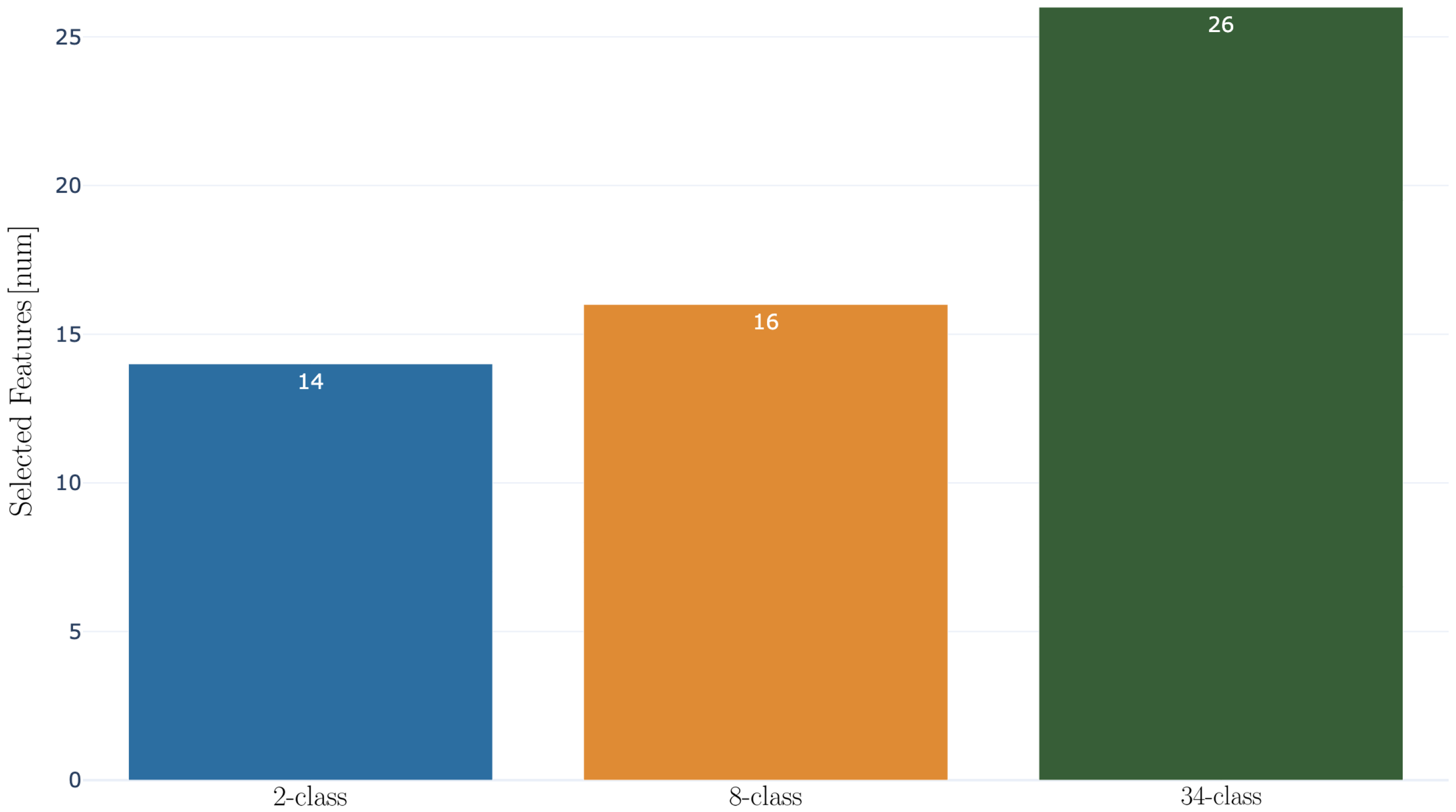
Overall, this approach was applied to all three versions of the dataset (2-class, 8-class, and 34-class), each characterized by distinct distributions of benign instances. Consequently, feature selection was performed separately for each version, with many features consistently identified as top contributors across all three datasets. As shown in Figure 3, increasing the number of classes requires retaining additional features to effectively correlate them with specific classes. This impacts both the size and complexity of the trained models, as a larger feature set can potentially result in a simpler model for classifying the attack.
In particular, the following features (from the list in Table 3) have been selected for each dataset:
  • 2-class dataset: rst count, urg count, Variance, Flow duration, Std, Radius, Covariance, Header Length, Max, ack flag number, AVG, Magnitude, HTTPS, Tot size.
  • 8-class dataset: Variance, RST count, URG count, Std, Radius, Magnitude, AVG, Tot size, Max, Min, Covariance, Protocol type, Flow duration, Header Length, Tot sum, ack flag number.
  • 34-class dataset: ICMP, fin flag number, Protocol Type, Variance, Header Length, syn flag number, rst count, Magnitude, AVG, Radius, Std, urg count, Min, Tot size, Max, Covariance, rst flag number, syn count, flow duration, TCP, psh flag number, Tot sum, UDP, fin count, ack flag number, ack count.

4.2. Hyperparammeter Optimization

With specific regard to DL models, it is well-known that hyperparameters, although remaining fixed during the training process, still play a crucial role in determining the model’s architecture and the overall performance efficiency. Consequently, an automatic tuning of categorical, discrete, and continuous hyperparameters is accomplished through a Hyperparammeter Optimization (HPO) task. More in detail, the primary goal of HPO is to identify the optimal hyperparameters’ set x by minimizing the chosen performance metric, i.e., as
x = arg min x X f ( x )
where x represents the optimal hyperparameters’ set, f ( x ) corresponds to the model’s performance metric evaluated on a validation set x X , and X denotes the hyperparameter search space, i.e., the set of all possible combinations of hyperparameter values.
Moreover, we consider a BO for hyperparameter tuning: this effectively enhances the performance of the evaluated DL models by systematically exploring the hyperparameters’ space and balancing both exploration and exploitation. On the operational side, the KerasTuner library [43] has been employed to effectively implement BO. For the sake of completeness, Table 8 presents the optimized parameters along with their defined ranges in the search space.

4.3. Model Training

In the following, we present the DL models that have been evaluated in this study, highlighting their strengths and limitations. For clarity and completeness, their shared general architecture is outlined in Figure 4.

4.3.1. SimpleRNN

SimpleRNN’s cells represent the most lightweight RNN layer, with a SimpleRNN’s layer featuring m hidden units, n features, and o outputs, taking an input x t R n at time t and processing it to produce an input activation equal to
a t = f input ( W x · x t + b x )
where W x R n × m is the input weight matrix; and b x R n is the bias vector.
Then, SimpleRNN updates the hidden state by using the previous state and the activation function as follows:
h t = f hidden ( W h · h t 1 + a t + b h )
where W h R m × m is the hidden weight matrix; and b h R m is the hidden state bias vector.
Finally, the output is calculated as
y t = f output ( W y · h t + b y )
where W y R m × o is the hidden-to-output weight matrix; and b y R o is the output bias vector. Note that, in our particular case, f input and f hidden correspond to the REctified Linear Unit (ReLU) activation function [44], while f output corresponds to the softmax function [45].
Moreover, unlike traditional FeedForward Networks (FFNs) [46], RNNs have connections forming cycles, allowing them to maintain hidden state information and capture temporal dependencies. RNNs are employed in tasks like Natural Language Processing (NLP), speech recognition, and time-series prediction. However, they face challenges like the vanishing gradient problem, which limits their ability to capture long-term dependencies [47].

4.3.2. Long Short-Term Memory (LSTM)

LSTM networks address the vanishing gradient problem afflicting the RNN models. In detail, LSTMs use memory cells with gates to regulate information flow, allowing them to capture and remember long-term dependencies in sequential data. An LSTM architecture typically consists of memory cells along with input, forget, and output gates. These components commonly use the sigmoid function ( σ ) as the recurrent activation and the hyperbolic tangent function (tanh) as the standard activation—in our implementation, the ReLU function is instead used as activation function. The architecture is based on the following layers:
i t = σ ( W i x · x t + W i h · h t 1 + b i ) f t = σ ( W f x · x t + W f h · h t 1 + b f ) g t = tanh ( W g x · x t + W g h · h t 1 + b g ) o t = σ ( W o x · x t + W o h · h t 1 + b o ) c t = f t · c t 1 + i t · g t h t = o t · tanh ( c t )
where i t ( 0 , 1 ) m is the input gate state; f t ( 0 , 1 ) m is the forget gate state; o t ( 0 , 1 ) m is the output gate state; c t R m is the cell state using the cell update g t ( 1 , 1 ) m ; and h t ( 1 , 1 ) m is the hidden state update. Input matrices W i x , W f x , W g x and W o x , associated with the input, have dimensions n × m ; hidden matrices W i h , W f h , W g h and W o h , associated with the previous hidden state, have dimensions m × m .
Finally, it is noteworthy to highlight that LSTMs excel in tasks involving time-series data, NLP, and speech recognition, making them suitable for applications requiring the modeling of intricate temporal relationships and handling of sequential patterns. Therefore, an adequate data processing is essential to prevent overfitting and to minimize computational complexity when using these models. Despite their effectiveness, they are susceptible to exploding gradients, particularly in regression problems [48].

4.3.3. Gated Recurrent Unit (GRU) and Bidirectional GRU

Similarly to LSTMs, GRUs offer an efficient solution for sequence modeling, exhibiting similar limitations to LSTM but benefiting from a simplified architecture, which makes them—in terms of both efficiency and complexity— more suitable to edge computing [49]. The difference between GRU and LSTM lies on the cells type, which involve the following operations:
z t = σ ( W z x · x t + W z h · h t 1 + b z ) r t = σ ( W r x · x t + W r h · h t 1 + b r ) h ˜ t = tanh ( W o x · x t + r t ( W o h · h t 1 ) + b o ) h t = ( 1 z t ) h t 1 + z t h ˜ t
where z t ( 0 , 1 ) m is the update gate; r t ( 0 , 1 ) m is the reset gate; h ˜ t R m , h t R m represent the candidate hidden state and hidden state update, respectively. Input matrices W z x , W r x and W o x , associated with the input layer, have dimensions n × m ; hidden matrices W z h , W r h and W o h , associated with the previous hidden state, have dimensions m × m .

4.3.4. Multi-Layer Perceptron (MLP)

MLP is the simplest FFN, composed of multiple neurons layers. Then, being trained using backpropagation, MLPs are versatile and employed in various applications, such as classification and regression tasks [50]. The architecture is based on the following layers:
Input Layer : h ( 1 ) = W ( 1 ) · x + b ( 1 ) Hidden Layers : h ( i ) = W ( i ) · h ( i 1 ) + b ( i ) , i = 2 , , N Output Layer : a ( N + 1 ) = W ( N + 1 ) · h ( N ) + b ( N + 1 ) y ^ = softmax ( a ( N + 1 ) )
where W ( 1 ) R n × m is the input weight matrix; b ( 1 ) R n is the input bias vector; W ( i ) R m × m is the hidden weight matrix; b ( i ) R m is the hidden bias vector, with i = 2 , , N ; W ( N + 1 ) R m × o is the output weight matrix; b ( N + 1 ) R o is the output bias vector.

4.3.5. 1-Dimensional CNN (1D-CNN)

CNNs are DL architectures designed for visual data processing, being highly effective for image data thanks to their ability in capturing spatial hierarchies. However, they can be used also for sequence classification by transforming data sequences using convolutional operations. Unfortunately, CNNs demand a high computational power and may impose some limitations on the time-series data in order to work properly [51]. For clarity, a 1D CNN can be analytically described as
Convolutional Layer : Z ( i ) = W ( i ) X ( i 1 ) + b ( i ) , A ( i ) = Activation ( Z ( i ) ) Pooling Layer : P ( i ) = MaxPooling ( A ( i ) ) Flatten Operation : P flat ( i ) = Flatten ( P ( i ) ) Fully Connected Layer : F ( i ) = W ( i ) · P flat ( i ) + b ( i ) , H ( i ) = Activation ( F ( i ) ) i = 1 , , N
where Z ( i ) R T i × F i denotes the pre-activation feature map obtained by convolving the input from the previous layer X ( i 1 ) R T i 1 × C i , with the weight matrix (or filter tensor) W ( i ) R F i × K i × C i via the convolution operator ⊛, and adding the bias vector b ( i ) R F i ; T i 1 is the temporal length of the input; C i is the number of input channels; F i is the number of convolutional filters; K i is the filter size, for layer i = 2 , , N . The activated feature map is given by A ( i ) R T i × F i , which is obtained by applying a non-linear activation function ϕ ( · ) (e.g., ReLU, sigmoid, tanh) to Z ( i ) . The pooled feature map is P ( i ) R T p , i × F i where the max-pooling operator selects, for each channel, the maximum value within each pooling window W k , according to MaxPooling ( A ( i ) ) k = max t W k A t ( i ) , thereby reducing the temporal resolution from T i to T p , i . The flattened representation P flat ( i ) R T p , i × F i is obtained by applying the vectorization operator, denoted as vec ( · ) , that re-arranges all the elements of P ( i ) into a one-dimensional vector. Finally, H ( i ) R D i is the activated output of the fully connected layer, where D i corresponds to the number of neurons in the layer.

4.3.6. Temporal Convolutional Network (TCN)

TCN is a particular 1D-CNN-based DL model proposed for processing sequential data and featuring three key features: (i) Causal Convolutions, preventing information leakage from future to past data and ensuring that predictions are made only on the basis of current and past data and are not influenced by future information; (ii) Dilated Convolutions, allowing the model to capture long-range temporal dependencies in the data and improving its ability to extract features from sequences; (iii) Flexible Sequence Length Handling, enabling TCN to process sequential data with any length and mapping them to output sequences with the same length [52].

4.4. Evaluation Metrics

In order to assess the performance of the chosen DL models on the selected dataset for the IDS of interest, the following evaluation metrics have been employed.

4.4.1. Accuracy

Accuracy (denoted as A ) measures the ratio between the number of correctly predicted instances and the total number of instances. It can be expressed as
A = TP + TN TP + TN + FP + FN
where TP, TN, FP, and FN represent the numbers of true positives, true negatives, false positives, and false negatives, respectively. The accuracy A ranges from 0 (with none of the instances being correctly classified) to 1 (with all instances being correctly classified). Although A is an indicator of the overall model performance, it may be misleading in the case of imbalanced datasets.

4.4.2. Precision

Precision (denoted as P ) indicates the ratio between the number of correctly predicted positive cases and the total number of positives. It can be expressed as
P = TP TP + FP .
The precision P ranges from 0 (worst case) to 1 (best case). Consequently, a high precision is associated with a low false positive rate, making it critical in applications where false positives are critical.

4.4.3. Recall

Recall (denoted as R and also as sensitivity) measures how effectively the model allows to detect truly positive instances. It can be defined as the ratio between the number of true positives and the sum between the number of true positives and false negatives (i.e., the number of all positives):
R = TP TP + FN .
The recall R ranges from 0 (worst case) to 1 (best case). Therefore, a high recall is essential when missing positive cases is detrimental, such as in medical diagnoses or intrusions detection.

4.4.4. F1-Score

The F1-Score (denoted as F ) balances precision P and recall R as follows:
F = 2 × P × R P + R = 2 × TP 2 × TP + FP + FN .
The F1-Score F ranges from 0 (if the precision P or the recall R is 0) to 1 (indicating perfect precision and recall). It is useful especially for imbalanced datasets, as it simultaneously takes into account both false positives and false negatives.

4.4.5. Matthews Correlation Coefficient (MCC)

The MCC is defined as follows:
M = ( TP × TN ) ( FP × FN ) ( TP + FP ) ( TP + FN ) ( TN + FP ) ( TN + FN ) .
Unlike the F1-Score, the MCC offers a more balanced perspective on the performance by incorporating all confusion matrix elements, with values ranging from 1 (no prediction at all) to + 1 (perfect prediction).
Unlike accuracy, the MCC is more robust in the case of imbalanced datasets.

4.4.6. Cohen’s Kappa Coefficient

The Cohen’s Kappa Coefficient [53] (denoted as κ ) is a statistical measure quantifying the agreement between predicted and actual labels, while adjusting for agreement occurring by chance. It is defined as follows:
κ = 2 × ( TP × TN FN × FP ) ( TP + FP ) × ( FP + TN ) + ( TP + FN ) × ( FN + TN ) .
Unlike accuracy, κ provides a more reliable evaluation in the presence of class imbalance. In fact, κ values range from 1 (complete disagreement) to + 1 (perfect agreement), where 0 indicates a random agreement. In other words, the best case is with | κ | close to 1.

4.4.7. Receiver Operating Characteristic (ROC) Curve and Area Under Curve (AUC)

The ROC curve r ( x ) is a function of a threshold x: more precisely, it returns the accuracy of a binary classifier deciding on the basis of the threshold x. It corresponds to the ratio between true positives and false positives, namely r ( x ) = TP / FP . The AUC can be expressed as follows:
AUC = 0 1 r ( x ) d x
where r ( x ) is the ROC curve. The AUC represents the model’s capability to distinguish between classes. In fact, a perfect classifier has an AUC equal to 1, while an AUC equal to  0.5 denotes a limited discrimination ability.

4.5. Model Complexity

In the following, the computational complexity of the considered models is evaluated in terms of three metrics, namely: (i) Multiply–ACCumulate operations (MACCs), (ii) RAM usage, and (iii) inference time. The evaluation has been conducted through the STMicroelectronics Cube.AI Analyzer tool [16], a cloud-based platform designed to assess the performance of ML/DL models on resource-constrained devices, with 32-bit floating point (FP32) models being deployed on a STM32H7S78-DK board [16] featuring a 600 MHz ARM Cortex-M7 microcontroller, 620 KB internal memory, and 16 MB external RAM.
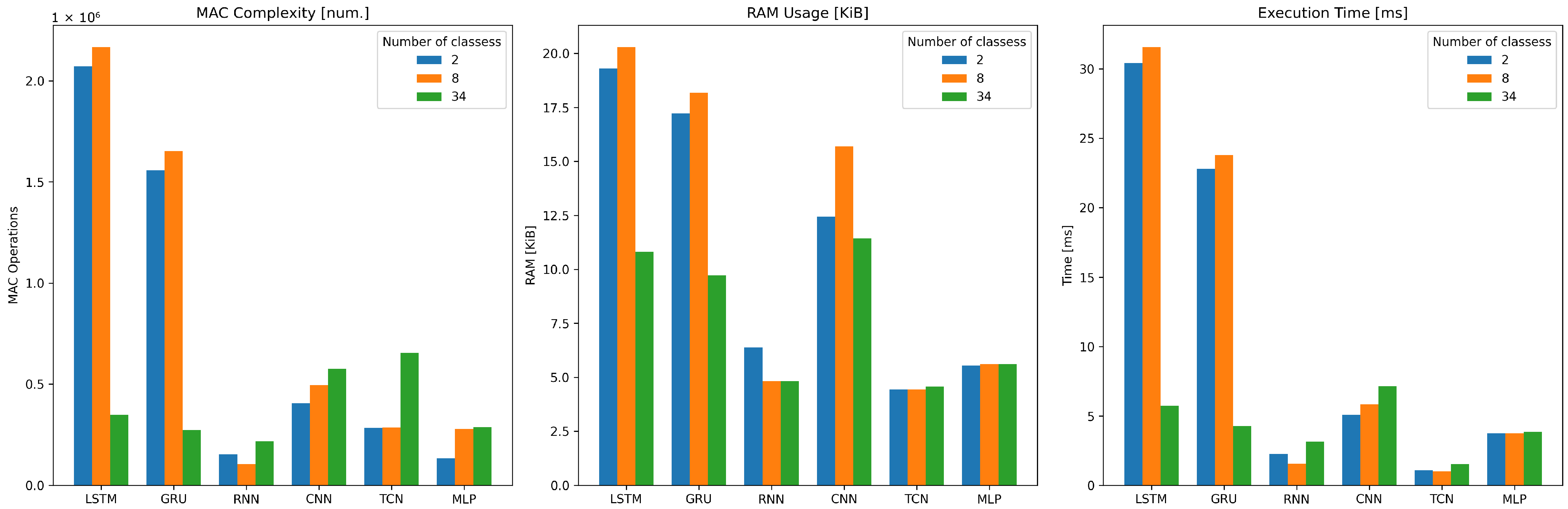
The obtained experimental results, shown in Figure 5 and detailed in Table 9 for clarity and completeness, indicate LSTM as the model which has the highest computational demand and requires substantially more MACCs and RAM than the other algorithms. In contrast, TCN and MLP exhibit the lowest average computational complexities, with TCN achieving a 94.61 % reduction in the inference time (if compared to LSTM) and using approximately 73 % less RAM than GRU. Similarly, MLP reduces the number of MACCs by 84.73 % in comparison to LSTM. This makes both TCN and MLP suitable for deployment on resource-constrained devices, where computational efficiency is fundamental.
Finally, it should be highlighted that the considered DL models have been evaluated not only on the basis of their accuracy in detecting several types of attacks, but also considering their deployability according to multiple computational metrics. To this end, given the challenges of deploying complex AI models on resource-constrained devices, an 8-bit integer (INT8) quantization of activations and weights has been applied to further reduce the computational complexity and enhance the efficiency. A detailed discussion of these quantization techniques and their impact on the performance is given in Section 5.2.

5. Results

In order to present the findings of the proposed experimental analysis, detailing the performance of each considered DL model discussed in Section 4.3, we first analyze each model’s ability to accurately classify network traffic, distinguishing between benign and malicious network activities. Then, we examine the models’ performance across different classes and levels of complexity, looking for the optimal configuration suitable for real-time IoT security applications. We recall the following:
  • The selected performance metrics are: accuracy A , precision P , recall R , F1-Score F , MCC M , and Cohen’s Kappa Coefficient κ .
  • The selected complexity evaluation metrics are: number of MACCs, RAM usage, and inference time.

5.1. Network Traffic Classification Performance

As shown in Table 10, LSTM achieves the highest performance in the context of 2-class ( C = 2 ) anomaly detection, providing the highest accuracy ( 99.37 % ) and showing high values of the other evaluation metrics. Instead, as shown in Table 11, LSTM still demonstrates slightly better results in the context of 8-class ( C = 8 ) anomaly detection, outperforming the other models in terms of accuracy, precision, recall, F1-score, Cohen’s Kappa Coefficient, and MCC. Finally, as detailed in Table 12, considering the more complex 34-class ( C = 34 ) anomaly detection task, MLP emerges as the top-performing model, achieving the highest accuracy, F1-score, Cohen’s Kappa Coefficient, MCC, and recall. Nevertheless, the differences (in terms of performance) returned by the models are minimal, showing that no single model consistently dominates across all the tasks. Therefore, the trade-off between computational efficiency and complexity should guide the model’s selection, in particular with regard to applications requiring a deployment on resource-constrained devices or real-time processing environments.
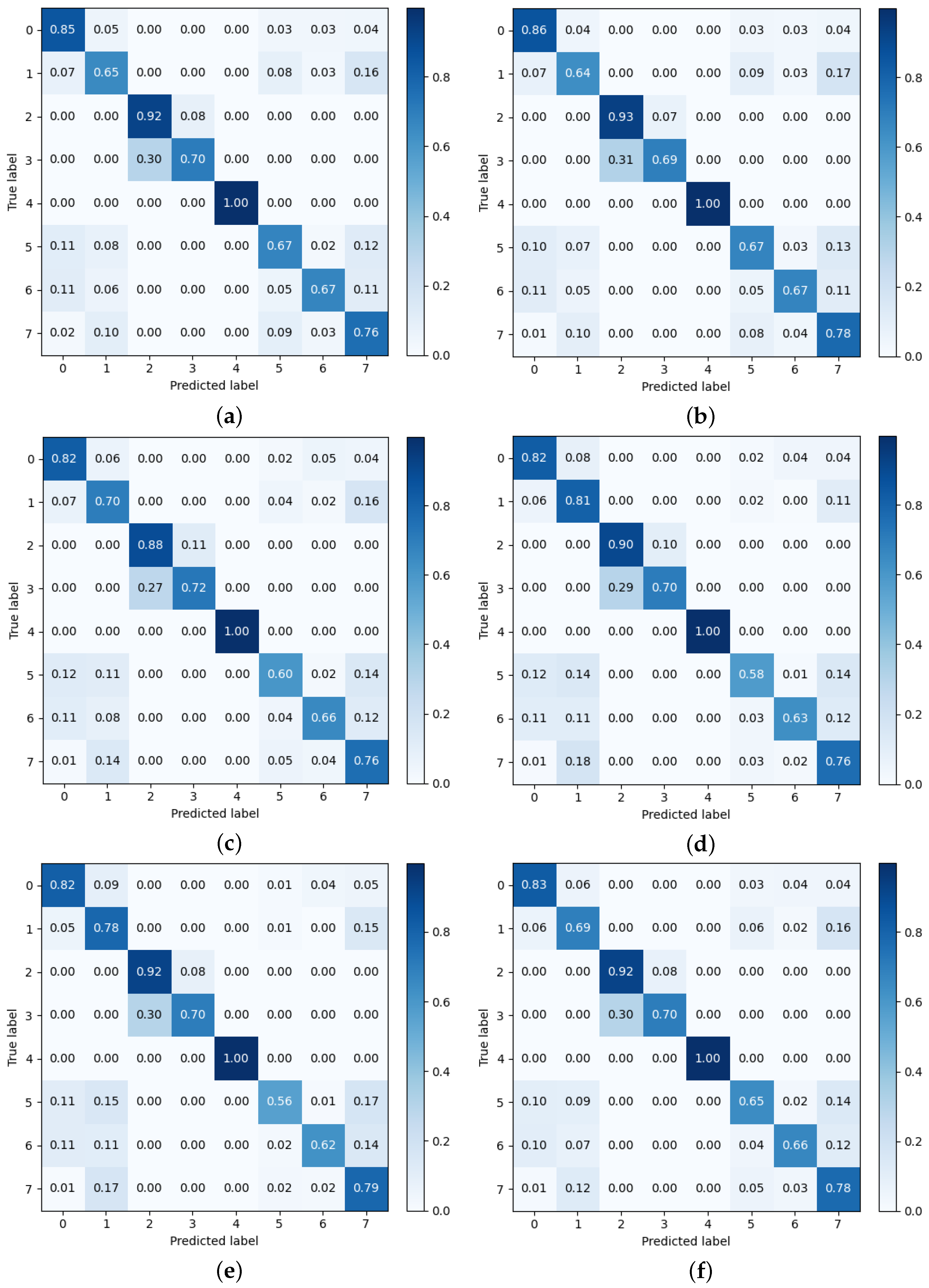
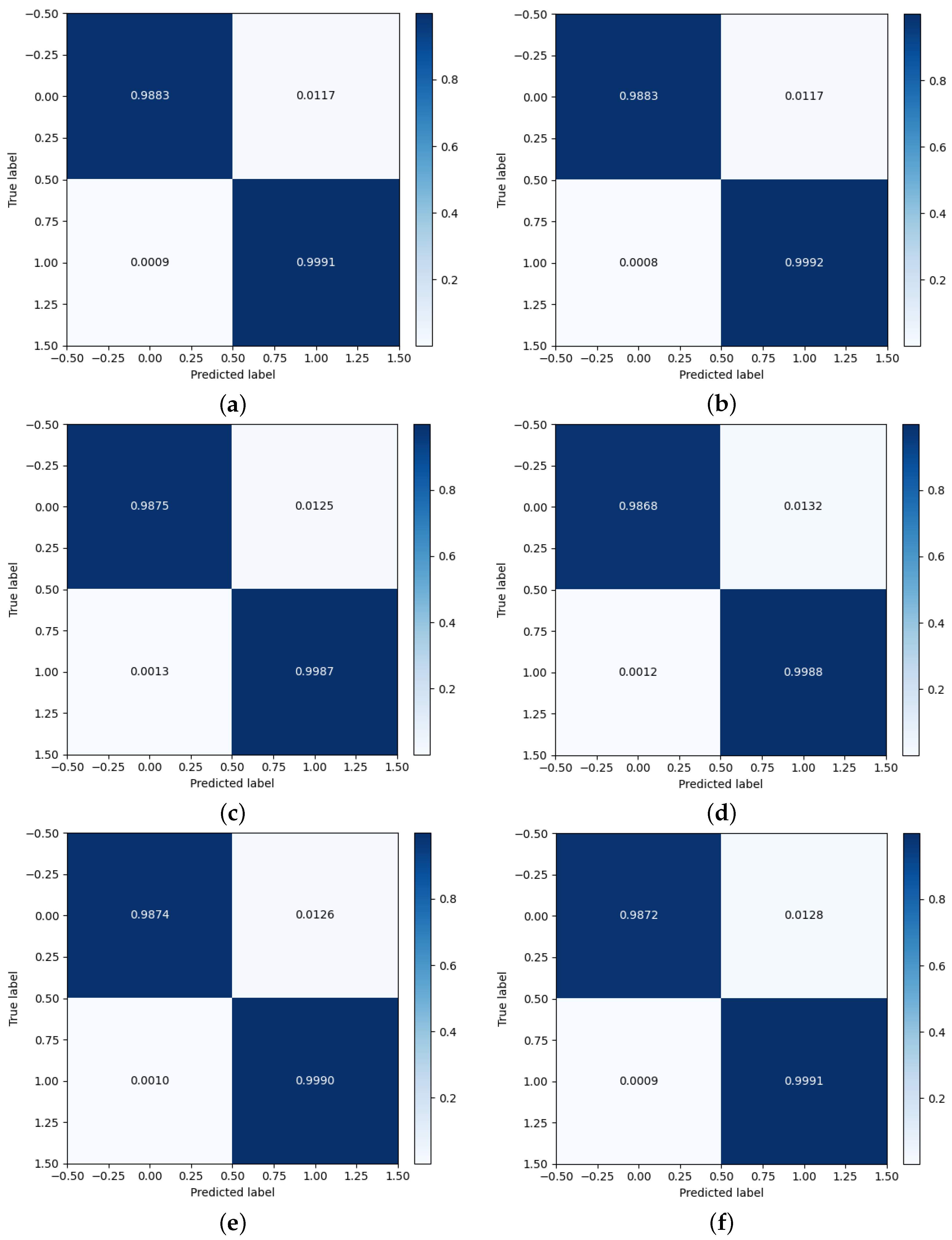
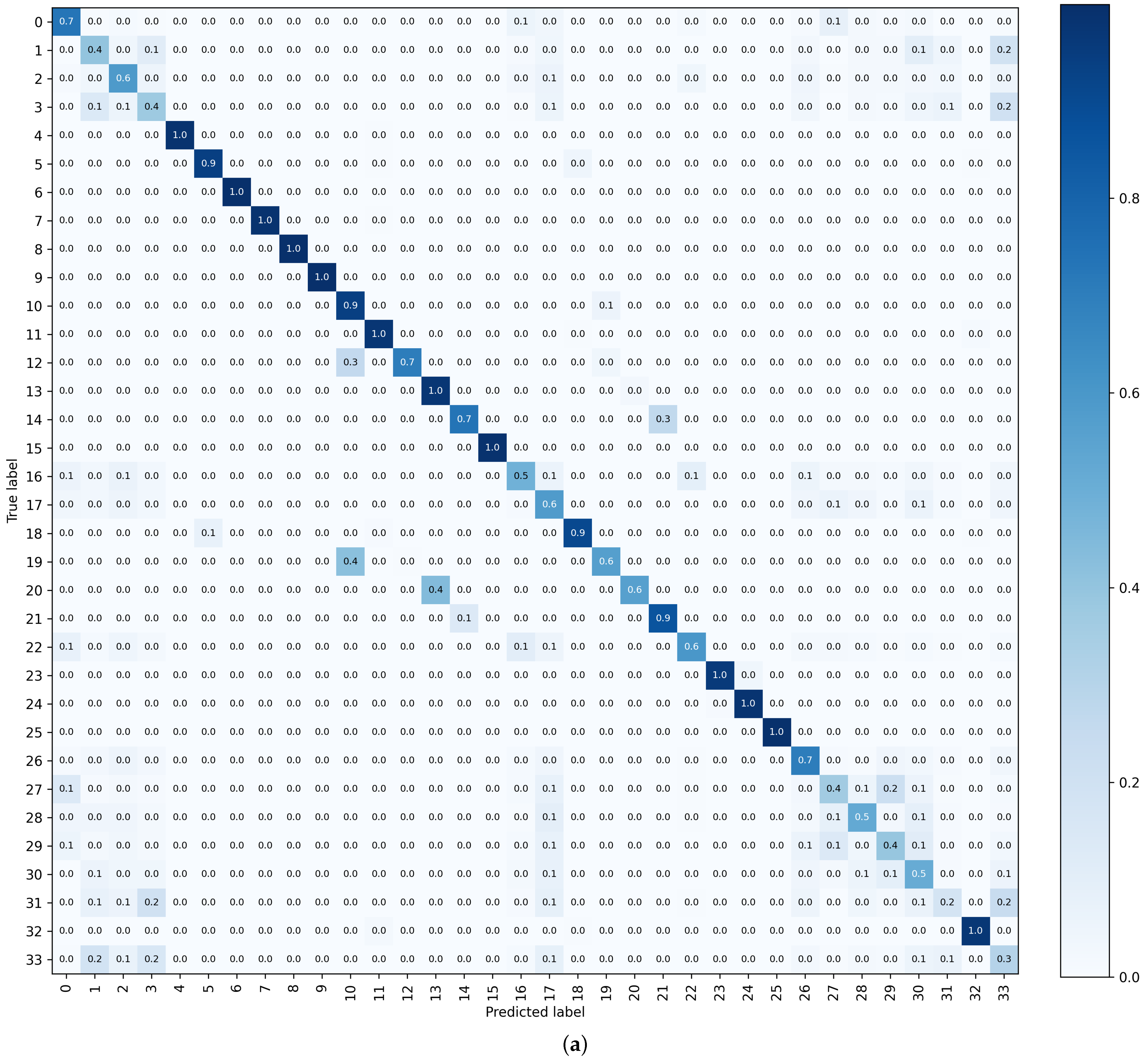
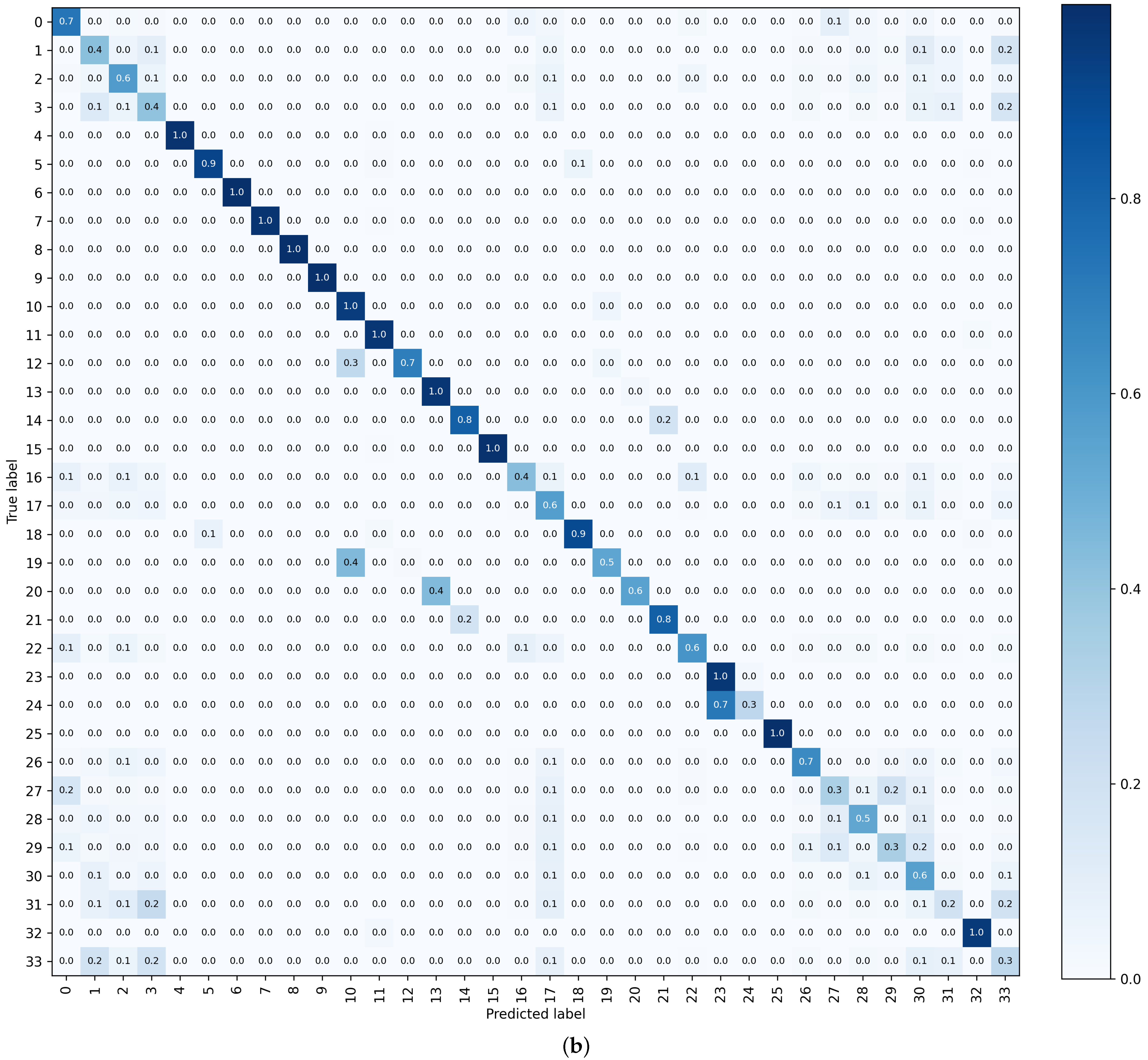
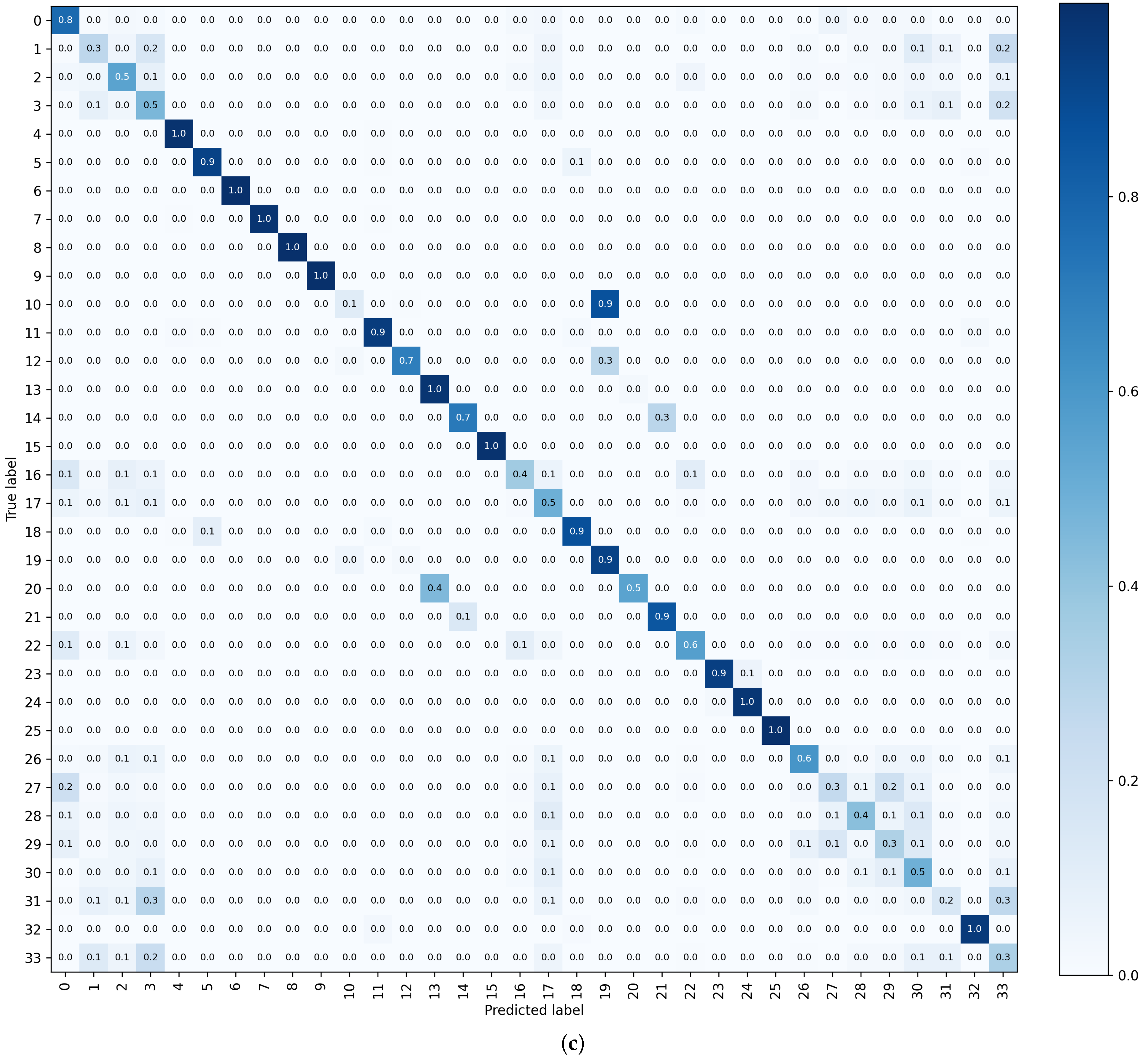
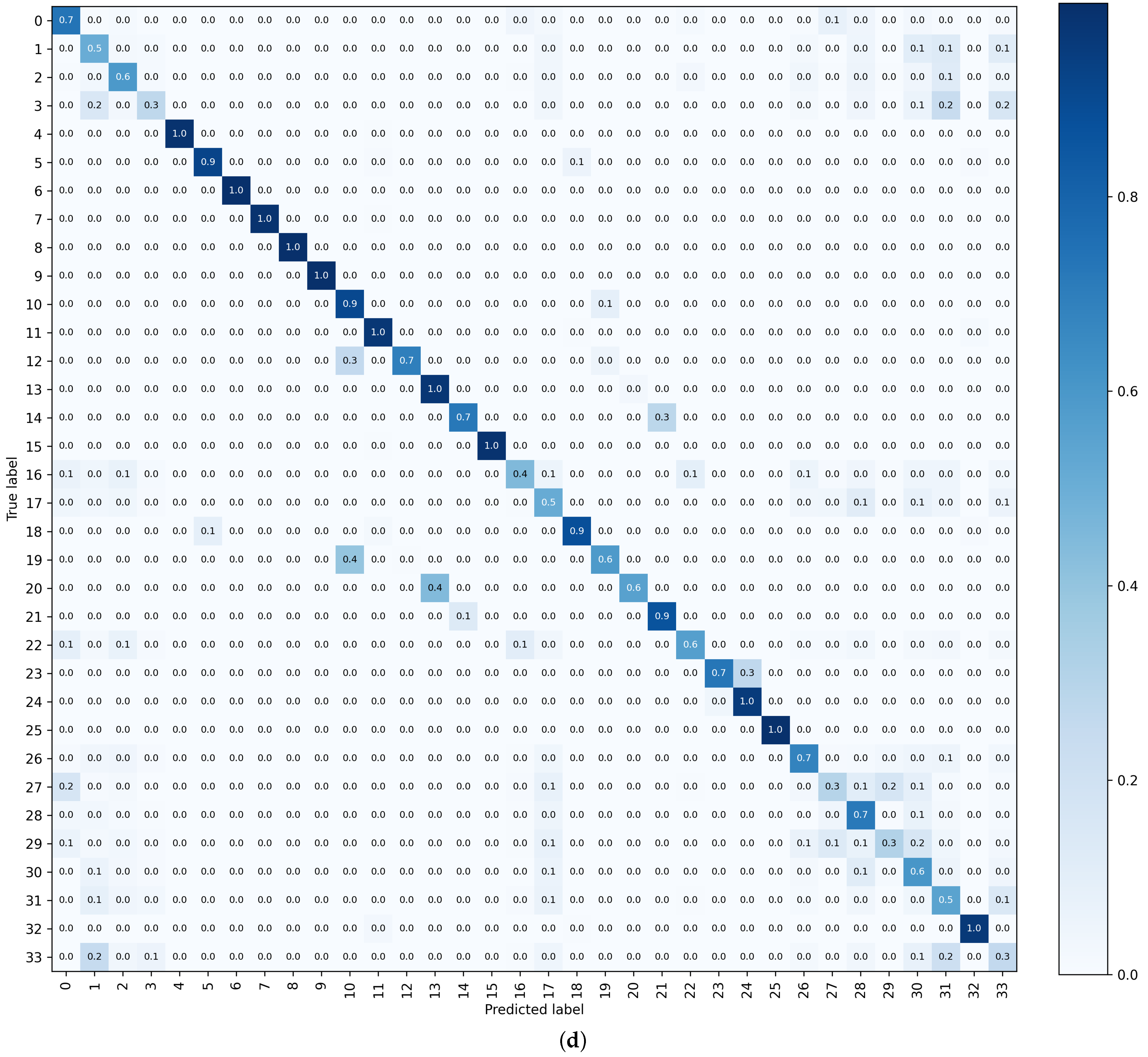
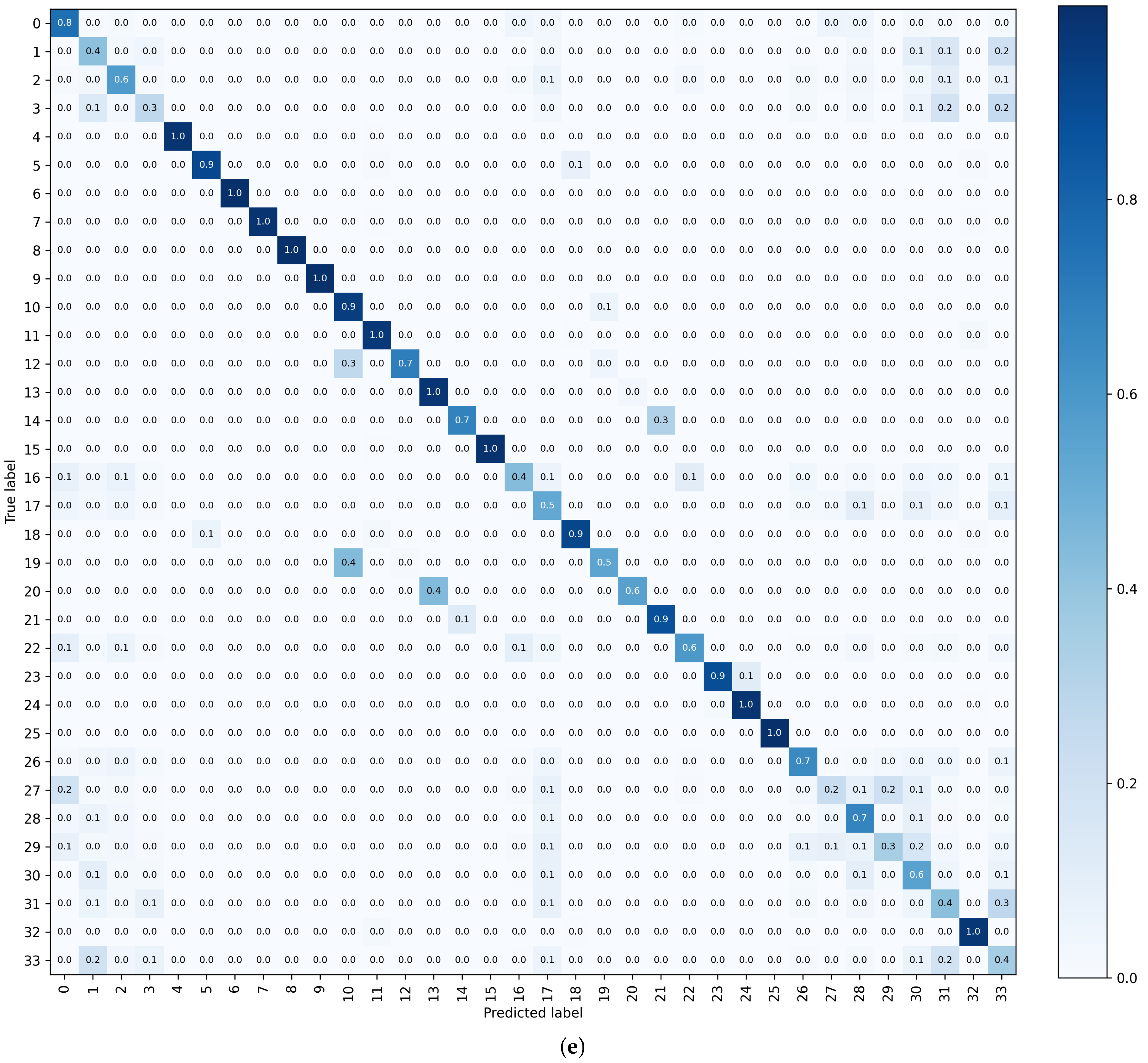
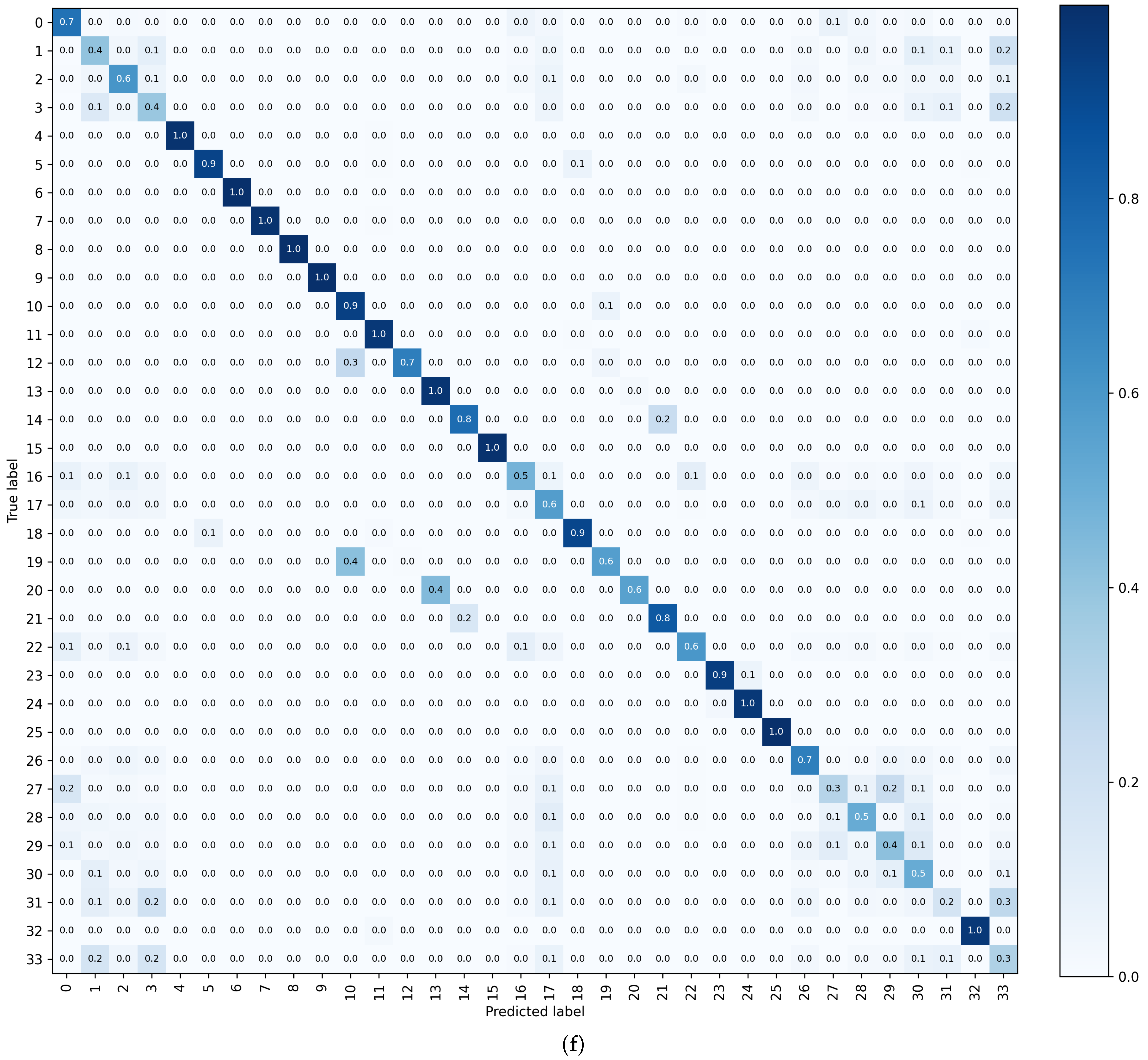
Then, in order to check the validity of the results not only on the basis of overall metrics, but also at class level, confusion matrices returned by 2-, 8-, and 34-class configurations, together with the mapping between attack classes and their corresponding numerical labels, are detailed in Appendix A.

5.2. Post-Training Quantization (PTQ)

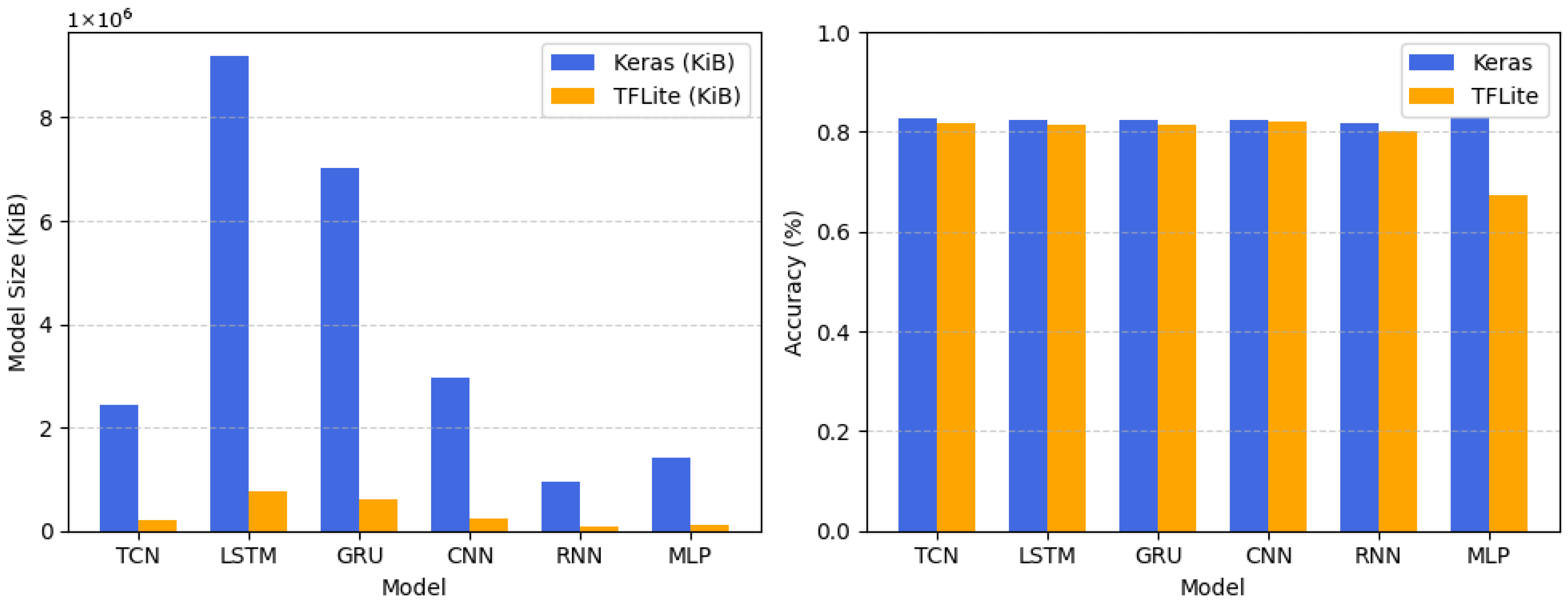
Since (as mentioned in Section 4) it is of interest to verify the deployability of the considered DL models on resource-constrained IoT devices, the application of a PTQ technique emerges as a highly effective mechanism to reduce the computational complexity and enhance the efficiency. In detail, PTQ specifically focuses on compressing pre-trained models for efficient deployment on tiny IoT devices by converting models’ weights from FP32 values to INT8 values, thus significantly reducing both model size and memory footprint and enhancing inference efficiency without requiring a re-training. On the operational side, we employ both Keras and TensorFlow Lite (TFlite) libraries, with PTQ compressing and quantizing the Keras model by converting it to the TFLite format, which, in turn, corresponds to a lightweight data representation useful for deploying ML and DL models on resource-constrained embedded devices [54].
After applying PTQ on the considered AI models, the obtained results are shown in Figure 6, where an average model size’s reduction of 91.24 % , with an average accuracy drop of only 4 % across all considered anomaly detection classes, is shown. This highlights the significance of quantization to optimize resource utilization and energy efficiency in constrained devices. In fact, quantizing CNNs to an 8-bit representation usually results in a slight performance degradation with the benefit of a significant memory utilization reduction [55].

5.3. Accuracy-Computational Complexity Trade-Off

In order to simultaneously evaluate both accuracy and computational complexity of the considered DL models, we define a new trade-off score, denoted as ψ , to provide a balanced assessment by considering normalized accuracy alongside computational complexity (including the number of MACCs, RAM usage, and execution time) [56]. In the following, we summarize the steps required to calculate ψ . We remind you that ψ is an effective evaluation metric in relative terms, i.e., it allows you to fairly compare a set of DL models among themselves. In other words, ψ does not represent an “absolute” performance metric of a single DL model.

5.3.1. Metrics Normalization

All the considered complexity metrics are normalized to the range [ 0 , 1 ] using the following min–max scaling strategy:
ϑ k ( norm ) ϑ k ϑ k ( min ) ϑ k ( max ) ϑ k ( min )
where k { macc , ram , itime } corresponds to the considered complexity metric (namely: number of MACCs, RAM usage, inference time, respectively); ϑ k represents the original value of the k-th complexity metric; ϑ k ( min ) and ϑ k ( max ) correspond to the minimum and maximum values of ϑ k across all considered DL models; ϑ k ( norm ) is the normalized value of the k-th complexity metric.

5.3.2. Efficiency Score Computation

In order to represent the computational complexity of each considered model, we introduce an efficiency score, denoted as ξ , defined as the following weighted average of the normalized complexity metrics (defined in Section 5.3.1):
ξ w macc · ϑ macc ( norm ) + w ram · ϑ ram ( norm ) + w itime · ϑ itime ( norm )
where w macc , w ram , and w itime represent the weights assigned to each complexity metric, respectively. In order to avoid a biased performance analysis, we assign the same weight to all considered complexity metrics, i.e., we set w macc = w ram = w itime = 1 / 3 .

5.3.3. Trade-Off Score

Finally, the trade-off score ψ , balancing the ratio between normalized accuracy ϑ A ( norm ) and efficiency score ξ , is defined as follows:
ψ ϑ A ( norm ) ξ .
According to the definition in (12), a high value of ψ is representative of a better performance jointly considering accuracy and computational resource utilization.
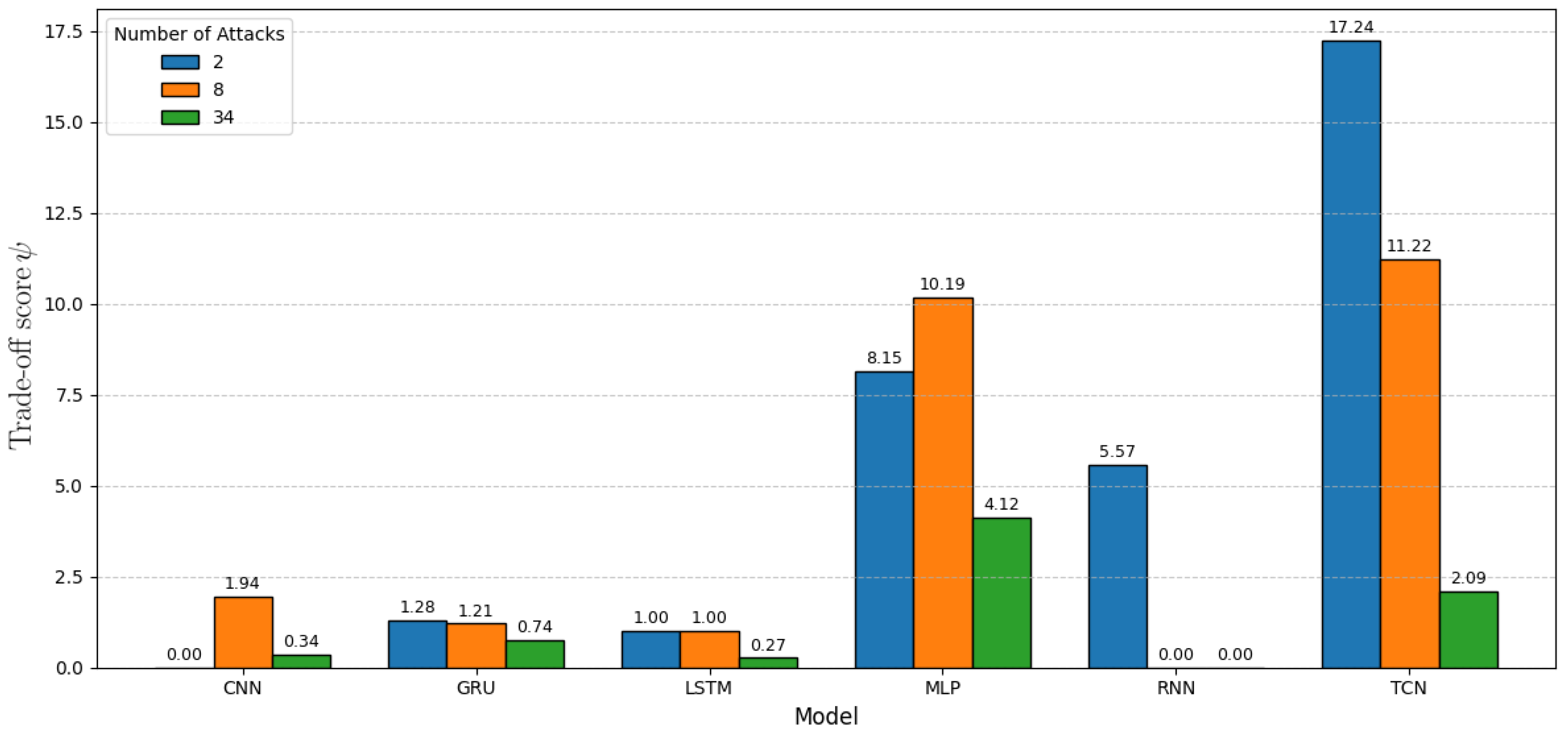
For completeness, the trade-off score ψ obtained by the considered DL models across the different datasets is shown in Figure 7. As can be observed, TCN emerges as the algorithm offering the most efficient balance between accuracy and computational complexity in the 2- and 8-class cases, i.e., in simple intrusion detection scenarios. In the more complex 34-class scenario, MLP is instead the algorithm returning the best trade-off.

5.4. Deployment on Resource-Constrained Devices

To evaluate the practical feasibility of deploying DL models on resource-constrained devices, quantized TCN and MLP models—being the best-performing models, according to the results shown in Section 5.3.3—were implemented and tested on the STM32H7S78-DK board, trying to assess how the number of output classes affects the algorithms’ computational and memory requirements when executed directly on the target HW.
In more detail, the complexity was analyzed in terms of the number of MACCs, RAM usage, and inference time, with these metrics obtained through on-board profiling tools and real-time measurements during the inference phase on the STM32H7S78-DK board. The obtained metrics are shown in Table 13, where 8-bit quantized (INT8) TCN and MLP models have been considered for the different output class configurations of interest—namely, for C { 2 , 8 , 34 } . For completeness, in Table 13 we also recall the accuracies of the algorithms.
For the sake of completeness, the relative percentage difference (denoted as Δ ϑ ) between the performance (for a given metric) returned by unquantized (FP32) and quantized (INT8) TCN and MLP models, considering the different output class configurations (namely, C { 2 , 8 , 34 } ), is shown in Table 14. In particular, this percentage difference is calculated as follows:
Δ ϑ k = ϑ k ( int 8 ) ϑ k ( fp 32 ) ϑ k ( fp 32 ) · 100
where k { A , macc , ram , itime , flash , msize } corresponds to the considered evaluation (either performance or complexity) metric (namely, accuracy, number of MACCs, RAM usage, inference time, flash usage, model size, respectively); ϑ k ( fp 32 ) and ϑ k ( int 8 ) represent the original value of the k-th metric returned by unquantized (FP32) and quantized (INT8) DL models, respectively. For better readability, instead of including the values of flash memory occupation and model size in Table 9 (for FP32 DL models) and Table 13 (for INT8 DL models), they have been included in Table 15 (columns 5–8).
As highlighted in Table 14, INT8 quantization produces a significant model size reduction for both TCN and MLP, exceeding 90 % in most cases. In particular, with regard to MLP, the number of MACCs remains essentially consistent (with variations smaller than 1 % ), the RAM usage increases moderately (between + 36 % and + 53 % ), the inference time decreases (between 16 % and 21 % ), and the flash usage is significantly reduced (between 71 % and 73 % ), thus reflecting lower weight storage needs. This highlights how dense layers (e.g., MLP) benefit from reduced computational cost and memory requirements (when quantized), thus leading to faster inference despite slightly higher RAM demands.
In contrast, TCN provides a different result. While model size is also reduced by more than 90 % and flash usage remains nearly constant, RAM usage and inference time of quantized versions increase substantially—between + 309 % and + 574 % , and between + 225 % and + 425 % , respectively. This behavior primarily occurs because TCN architectures, in particular one-dimensional convolutional layers, cannot be fully quantized to INT8, while, instead, MLP supports complete INT8 quantization. This is particularly evident given the type of MACCs shown in Table 15 as follows:
  • smul_f32_f32 performs a scalar multiplication between two FP32 values;
  • op_f32_f32 represents a generic operation—such as addition, activation, or normalization—applied to FP32 data;
  • smul_s8_s8 and op_s8_s8 perform, adopting signed INT8 data types, the same operations operated by MACCs 1 and 2;
  • smul_s8_f32 and smul_f32_s8 perform conversions from signed INT8 to FP32 and vice versa.
Thus, it is clear how TCN limitations in INT8 quantization arise because of an increased internal complexity—in terms of additional layers and MACCs, mainly dilated convolutions and dynamic padding—being not supported in integer form by both TensorFlow Lite and Cube-AI [57] from STMicroelectronics [58]. This leads to an unexpected increase in both RAM and flash memory usage, since several conversion and intermediate operations (to bridge between FP32 and INT8 arithmetic) are required during the quantization task. Specifically, the following apply:
  • As indicated by the operations’ breakdown, the bulk of the computation still relies on FP32 multiplications (namely, smul _ f 32 _ f 32 ), with several conversion layers having to be added before and after convolutional and element-wise operations (e.g., smul _ s 8 _ f 32 and smul _ f 32 _ s 8 ).
  • Each additional layer requires temporary buffers to store intermediate activations in both FP32 and INT8 formats: this drastically increases the RAM consumption at runtime, and in the worst case, the device has insufficient internal RAM, temporary buffers have to be stored into external RAM, and the performance degrades much more.
  • Each quantized layer needs to store its scale and zero-point parameters for proper rescaling between quantized tensors: this results in the need to add metadata that partially hinders the expected flash memory reduction. Moreover, as discussed for RAM, in the case of insufficient internal flash memory, an external memory should be used, further degrading the performance.
The final result is that, even though quantization decreases the overall weight storage by about 90 % , the proliferation of intermediate buffers and conversion operations results in higher runtime memory demands and slightly larger flash usage—especially in architectures which make extensive use of convolutional and residual connections, e.g., TCN.
Overall, the obtained results highlight that INT8 quantization effectively reduces model and memory requirements for embedded deployment, while its impact on RAM and inference time depends on the specific model architecture. Comparing the accuracy of FP32 and INT8 implementations of MLP and TCN models for all classes, it can be seen (from Table 14) that the accuracy loss due to quantization is negligible in binary anomaly detection ( C = 2 ), but increases when multiple classes (namely, C { 8 , 34 } ) are considered.

5.5. Quantized Models Accuracy-Computational Complexity Trade-Off

Finally, we evaluate the performance of quantized TCN and MLP models on the anomaly detection task using the trade-off score ψ . For the 2-class task, both TCN and MLP models achieve high accuracy (above 99 % ), with TCN slightly outperforming MLP, albeit with higher resource usage due to mixed-precision quantization (as discussed in Section 5.4). Then, as the task complexity increases (with 8-class and 34-class configurations), TCN maintains significantly higher accuracy and trade-off score, whereas the fully quantized MLP sacrifices accuracy in exchange for reduced model size and complexity.

5.6. Limitations of the Proposed Work

Finally, for the sake of clarity and completeness, it might be useful to highlight that, despite the promising performance of the proposed IDS and the consequent HW-aware evaluation, the following limitations emerge from our experimental analysis:
  • Quantization support for complex architectures: While MLP models can be fully quantized to INT8 with minimal impact on performance, TCN architectures suffer from incomplete quantization due to the presence of dilated convolutions and dynamic padding. This leads to increased RAM usage (up to + 574 % ) and inference time (up to + 425 % ) despite significant reductions in model size.
  • Trade-off between accuracy and computational efficiency: Although quantization reduces model size and flash usage, the accuracy of fully quantized MLP models decreases slightly (average drop 4 % ), highlighting the trade-off between resource efficiency and detection performance, in particular for multi-class ( C = 34 ) scenarios.
  • Scope of the evaluation: The study focuses on a single constrained platform (STM32H7S78-DK) and FP32-to-INT8 quantization schemes. Results may differ on alternative HW platforms, bit-widths, or DL frameworks, limiting the generality of the deployment conclusions.

6. Conclusions

The proposed study focuses on the integration of IDSs in IoT networks to protect against increasingly sophisticated threats targeting connected IoT devices. In particular, different DL models—namely, LSTM, GRU, RNN, CNN, TCN, and MLP—have been evaluated over a publicly available dataset (namely, CICIoT2023) including network traffic traces comprising different attack classes, for anomaly detection on resource-constrained IoT devices. Then, BO has been applied to optimize the hyperparameters of the considered DL models, which have then been evaluated for both binary (2-class) and multi-class (8-class, 34-class) intrusion detection tasks. The models’ performance has been assessed on an STM32H7S78-DK board (virtually available through the cloud-based STM Cube.AI Analyzer tool) considering the number of MACCs, RAM usage, and inference time as computational complexity metrics. Then, their deployability on resource-constrained IoT devices has been evaluated by introducing a trade-off score ψ , balancing both classification accuracy and computational complexity, obtaining that TCN and MLP guarantee the most efficient balance with respect to the other DL models, on the basis of the specific intrusion detection task. Furthermore, PTQ has been considered in order to evaluate the impact, on both model size and classification accuracy, of parameter quantization (from FP32 to INT8). The obtained experimental results demonstrate a significant model size reduction (greater than 80 % ) for both TCN and MLP with all considered classes. However, there are differences between TCN and MLP: Models based on dense layers (such as MLP) benefit from lower computational costs and memory requirements after quantization; convolution-based models (such as TCN), instead, exhibit increased runtime and RAM usage—particularly when the number of output classes grows—while showing only a marginal increase in the number of MACCs. These findings highlight that post-training INT8 quantization should be applied by taking into account the considered model and the final goal (e.g., latency or computational complexity).   

Author Contributions

Conceptualization, A.M., D.A., L.D. and G.F.; methodology, A.M., D.A., L.D. and G.F.; software, A.M. and D.A.; validation, A.M., D.A., L.D. and G.F.; formal analysis, A.M., D.A., L.D. and G.F.; investigation, A.M., D.A., L.D. and G.F.; resources, A.M. and D.A.; data curation, A.M., D.A., L.D. and G.F.; writing—original draft preparation, A.M., D.A., L.D. and G.F.; writing—review and editing, A.M., D.A., L.D. and G.F.; visualization, A.M., D.A., L.D. and G.F.; supervision, L.D. and G.F.; project administration, L.D. and G.F.; funding acquisition, L.D. and G.F. All authors have read and agreed to the published version of the manuscript.

Funding

This work was partially supported by the European Union’s Horizon Europe research and innovation program Key Digital Technology (KDT) Joint Undertaking (JU) under grant agreement No. 101097267, OPEVA project—“OPtimization of Electric Vehicle Autonomy,” and grant agreement No. 101139769, DistriMuSe project—“Distributed Multi-Sensor Systems for Human Safety and Health.” This work was also partially supported by the European Union—Next Generation EU under the Italian National Recovery and Resilience Plan (NRRP), Mission 4, Component 2, Investment 1.3, CUP J33C22002880001, partnership on “Telecommunications of the Future” (PE00000001—program “RESTART”), and by the Italian Complementary National Plan (PNC)–I.1 “Research initiatives for innovative technologies and pathways in the health and welfare sector,” D.D. 931 of 06/06/2022, the “DigitAl lifelong pRevEntion” (DARE) initiative, code PNC0000002, CUP B53C22006240001. The KDT JU received support from the European Union’s Horizon Europe research and innovation programme and the nations involved in the mentioned projects. The work reflects only the authors’ views; the European Commission is not responsible for any use that may be made of the information it contains.

Institutional Review Board Statement

Not applicable.

Informed Consent Statement

Not applicable.

Data Availability Statement

The data presented in this study have been derived from the public dataset “CICIoT2023: A Real-Time Dataset and Benchmark for Large-Scale Attacks in IoT Environment” at https://doi.org/10.3390/s23135941.

Conflicts of Interest

The authors declare no conflicts of interest. The funders had no role in the design of the study; in the collection, analyses, or interpretation of data; in the writing of the manuscript; or in the decision to publish the results.

Abbreviations

    The following abbreviations are used in this manuscript:
1D-CNNOne-dimensional Convolutional Neural Network
AUCArea Under Curve
DDoSDistributed DoS
DLDeep Learning
DNNDeep Neural Network
DoSDenial of Service
DTDecision Tree
FFNFeedForward Network
FLFederated Learning
GRUGated Recurrent Unit
HPOHyper-Parameter Optimization
IDSIntrusion Detection System
IoTInternet of Things
LGBMLight Gradient Boosting Machine
LSTMLong Short-Term Memory
MACCMultiply–ACCumulate operation
MCCMatthews Correlation Coefficient
MITMMan-in-the-Middle
MLMachine Learning
MLPMulti-Layer Perceptron
NLPNatural Language Processing
PTQPost-Training Quantization
ReLUREctified Linear Unit
RFRandom Forest
ROCReceiver Operating Characteristic
SDNSoftware-Defined Networking
SGDStochastic Gradient Descent
SimpleRNNSimple Recurrent Neural Network
SMOTESynthetic Minority Oversampling Technique
SVMSupport Vector Machine
TCNTemporal Convolutional Network
TFliteTensorFlow Lite
XSSCross-Site Scripting

Appendix A. Confusion Matrices of the Considered DL Models

As detailed in Section 5.1, in the following the confusion matrices returned by 2-, 8-, and 34-class configurations, are shown in Figure A1, Figure A2, and Figure A3, respectively, along with the corresponding mapping between attack classes and their corresponding numerical labels, listed in Table A1, Table A2, and Table A3, respectively.
Figure A1. Confusion matrices returned by the considered FP32 DL models in the 2-class ( C = 2 ) anomaly detection: (a) LSTM, (b) GRU, (c) RNN, (d) CNN, (e) TCN, (f) MLP.
Futureinternet 18 00034 g0a1
Table A1. Label encoding for the binary ( C = 2 ) classification.
ClassLabelClassLabel
Attack0Benign1
Figure A2. Confusion matrices returned by the considered FP32 DL models in the 8-class ( C = 8 ) anomaly detection: (a) LSTM, (b) GRU, (c) RNN, (d) CNN, (e) TCN, (f) MLP.
Futureinternet 18 00034 g0a2
Table A2. Label encoding for the 8-class ( C = 8 ) classification.
ClassLabelClassLabelClassLabel
Benign0DoS3Spoofing6
Brute Force1Mirai4Web-based7
DDoS2Reconnaissance5
Figure A3. Confusion matrices returned by the considered FP32 DL models in the 34-class ( C = 34 ) anomaly detection: (a) LSTM, (b) GRU, (c) RNN, (d) CNN, (e) TCN, (f) MLP.
Futureinternet 18 00034 g0a3aFutureinternet 18 00034 g0a3bFutureinternet 18 00034 g0a3cFutureinternet 18 00034 g0a3dFutureinternet 18 00034 g0a3eFutureinternet 18 00034 g0a3f
Table A3. Label encoding for the 34-class ( C = 34 ) classification.
ClassLabelClassLabelClassLabel
Benign0DDoS-SynonymousIP Flood12Mirai-greeth flood23
Backdoor Malware1DDoS-TCP Flood13Mirai-greip flood24
Browser Hijacking2DDoS-UDP Flood14Mirai-udpplain25
Command Injection3DDoS-UDP Fragmentation15Recon-Host Discovery26
DDoS-ACK Fragmentation4DNS Spoofing16Recon-OS Scan27
DDoS-HTTP Flood5Dictionary Brute Force17Recon-Ping Sweep28
DDoS-ICMP Flood6DoS-HTTP Flood18Recon-Port Scan29
DDoS-ICMP Fragmentation7DoS-SYN Flood19SQL Injection30
DDoS-PSHACK Flood8DoS-TCP Flood20Uploading Attack31
DDoS-RSTFIN Flood9DoS-UDP Flood21Vulnerability Scan32
DDoS-SYN Flood10MITMArp Spoofing22XSS33
DDoS-SlowLoris11

References

  1. Rejeb, A.; Suhaiza, Z.; Rejeb, K.; Seuring, S.; Treiblmaier, H. The Internet of Things and the Circular Economy: A Systematic Literature Review and Research Agenda. J. Clean. Prod. 2022, 350, 131439. [Google Scholar] [CrossRef] [Scilit]
  2. Hirsch, C.; Davoli, L.; Grosu, R.; Ferrari, G. DynGATT: A Dynamic GATT-based Data Synchronization Protocol for BLE Networks. Comput. Netw. 2023, 222, 109560. [Google Scholar] [CrossRef] [Scilit]
  3. Davoli, L.; Belli, L.; Cilfone, A.; Ferrari, G. Integration of Wi-Fi Mobile Nodes in a Web of Things Testbed. ICT Express 2016, 2, 95–99. [Google Scholar] [CrossRef] [Scilit]
  4. Pagliari, E.; Davoli, L.; Ferrari, G. Harnessing Communication Heterogeneity: Architectural Design, Analytical Modeling, and Performance Evaluation of an IoT Multi-Interface Gateway. IEEE Internet Things J. 2024, 11, 8030–8051. [Google Scholar] [CrossRef] [Scilit]
  5. Premalatha, B.; Prakasam, P. A Review on FoG Computing in 5G Wireless Technologies: Research Challenges, Issues and Solutions. Wirel. Pers. Commun. 2024, 134, 2455–2484. [Google Scholar] [CrossRef] [Scilit]
  6. Salsano, S.; Veltri, L.; Davoli, L.; Ventre, P.L.; Siracusano, G. PMSR–Poor Man’s Segment Routing, a Minimalistic Approach to Segment Routing and a Traffic Engineering Use Case. In Proceedings of the 2016 IEEE/IFIP Network Operations and Management Symposium (NOMS), Istanbul, Turkey, 25–29 April 2016; pp. 598–604. [Google Scholar] [CrossRef] [Scilit]
  7. Zikria, Y.B.; Ali, R.; Afzal, M.K.; Kim, S.W. Next-Generation Internet of Things (IoT): Opportunities, Challenges, and Solutions. Sensors 2021, 21, 1174. [Google Scholar] [CrossRef] [Scilit]
  8. Belli, L.; Cirani, S.; Davoli, L.; Ferrari, G.; Melegari, L.; Picone, M. Applying Security to a Big Stream Cloud Architecture for the Internet of Things. Int. J. Distrib. Syst. Technol. (IJDST) 2016, 7, 37–58. [Google Scholar] [CrossRef] [Scilit]
  9. Heidari, A.; Jabraeil Jamali, M.A. Internet of Things Intrusion Detection Systems: A Comprehensive Review and Future Directions. Clust. Comput. 2022, 26, 3753–3780. [Google Scholar] [CrossRef] [Scilit]
  10. Jiang, X.; Lora, M.; Chattopadhyay, S. An Experimental Analysis of Security Vulnerabilities in Industrial IoT Devices. ACM Trans. Internet Technol. 2020, 20, 16. [Google Scholar] [CrossRef] [Scilit]
  11. Bertino, E.; Islam, N. Botnets and Internet of Things Security. Computer 2017, 50, 76–79. [Google Scholar] [CrossRef] [Scilit]
  12. Khan, M.A.; Salah, K. IoT Security: Review, Blockchain Solutions, and Open Challenges. Future Gener. Comput. Syst. 2018, 82, 395–411. [Google Scholar] [CrossRef] [Scilit]
  13. Davoli, L.; Protskaya, Y.; Veltri, L. An Anonymization Protocol for the Internet of Things. In Proceedings of the 2017 International Symposium on Wireless Communication Systems (ISWCS), Bologna, Italy, 28–31 August 2017; pp. 459–464. [Google Scholar] [CrossRef] [Scilit]
  14. Asharf, J.; Moustafa, N.; Khurshid, H.; Debie, E.; Haider, W.; Wahab, A. A Review of Intrusion Detection Systems Using Machine and Deep Learning in Internet of Things: Challenges, Solutions and Future Directions. Electronics 2020, 9, 1177. [Google Scholar] [CrossRef] [Scilit]
  15. Neto, E.C.P.; Dadkhah, S.; Ferreira, R.; Zohourian, A.; Lu, R.; Ghorbani, A.A. CICIoT2023: A Real-Time Dataset and Benchmark for Large-Scale Attacks in IoT Environment. Sensors 2023, 23, 5941. [Google Scholar] [CrossRef] [Scilit] [PubMed]
  16. STMicroelectronics. Discovery Kit with STM32H7S7L8 MCU. Available online: https://www.st.com/en/evaluation-tools/stm32h7s78-dk.html (accessed on 1 January 2026).
  17. Abbas, S.; Bouazzi, I.; Ojo, S.; Al Hejaili, A.; Sampedro, G.A.; Almadhor, A.; Gregus, M. Evaluating Deep Learning Variants for Cyber-Attacks Detection and Multi-Class Classification in IoT Networks. Peerj Comput. Sci. 2024, 10, e1793. [Google Scholar] [CrossRef] [Scilit] [PubMed]
  18. Abbas, S.; Al Hejaili, A.; Sampedro, G.A.; Abisado, M.; Almadhor, A.S.; Shahzad, T.; Ouahada, K. A Novel Federated Edge Learning Approach for Detecting Cyberattacks in IoT Infrastructures. IEEE Access 2023, 11, 112189–112198. [Google Scholar] [CrossRef] [Scilit]
  19. Vajrobol, V.; Gupta, B.B.; Gaurav, A.; Chuang, H.M. Adversarial Learning for Mirai Botnet Detection based on Long Short-Term Memory and XGBoost. Int. J. Cogn. Comput. Eng. 2024, 5, 153–160. [Google Scholar] [CrossRef] [Scilit]
  20. Gharaibeh, H.; Aljaidi, M.; Nasayreh, A.; Al-Na’amneh, Q.; Jaradat, A.S.; Samara, G.; Al Mamlook, R.E. Deep Feature Extraction Framework Based on DNN for Enhancing Mirai Attachment Classification in Machine Learning. In Proceedings of the 2023 2nd International Engineering Conference on Electrical, Energy, and Artificial Intelligence (EICEEAI), Zarqa, Jordan, 27–28 December 2023; pp. 1–5. [Google Scholar] [CrossRef] [Scilit]
  21. Becerra-Suarez, F.L.; Tuesta-Monteza, V.A.; Mejia-Cabrera, H.I.; Arcila-Diaz, J. Performance Evaluation of Deep Learning Models for Classifying Cybersecurity Attacks in IoT Networks. Informatics 2024, 11, 32. [Google Scholar] [CrossRef] [Scilit]
  22. Aguru, A.D.; Erukala, S.B. A Lightweight Multi-Vector DDoS Detection Framework for IoT-enabled Mobile Health Informatics Systems using Deep Learning. Inf. Sci. 2024, 662, 120209. [Google Scholar] [CrossRef] [Scilit]
  23. Kumar, A.G.; Rastogi, A.; Ranga, V. Evaluation of Different Machine Learning Classifiers on New IoT Dataset CICIoT2023. In Proceedings of the 2024 International Conference on Intelligent Systems for Cybersecurity (ISCS), Gurugram, India, 3–4 May 2024; pp. 1–6. [Google Scholar] [CrossRef] [Scilit]
  24. Diab, A.; Chehade, A.; Ragusa, E.; Gastaldo, P.; Zunino, R.; Baghdadi, A.; Rizk, M. Intrusion Detection on Resource-Constrained IoT Devices with Hardware-Aware ML and DL. arXiv 2025, arXiv:2512.02272. [Google Scholar]
  25. Saxe, J.; Berlin, K. Deep Neural Network based Malware Detection using Two Dimensional Binary Program Features. In Proceedings of the 2015 10th International Conference on Malicious and Unwanted Software (MALWARE), Fajardo, PR, USA, 20–22 October 2015; pp. 11–20. [Google Scholar] [CrossRef] [Scilit]
  26. The Imbalanced-Learn Developers. RandomOverSampler. Available online: https://imbalanced-learn.org/stable/references/generated/imblearn.over_sampling.RandomOverSampler.html (accessed on 1 January 2026).
  27. Thapa, S.; Poudel, S.; Abouyoussef, M. TinyML-Enabled Intrusion Detection for Securing Electric Vehicle Supply Equipment (EVSE). In Proceedings of the 2025 1st International Conference on Secure IoT, Assured and Trusted Computing (SATC), Dayton, OH, USA, 25–27 February 2025; pp. 1–5. [Google Scholar] [CrossRef] [Scilit]
  28. Buedi, E.D.; Ghorbani, A.A.; Dadkhah, S.; Ferreira, R.L. Enhancing EV Charging Station Security Using a Multi-dimensional Dataset: CICEVSE2024. In Proceedings of the Data and Applications Security and Privacy XXXVIII, San Jose, CA, USA, 15–17 July 2024; pp. 171–190. [Google Scholar] [CrossRef] [Scilit]
  29. Arcot, S.; Masum, M.; Kader, M.S.; Saha, A.; Chowdhury, M. TinyML for Cybersecurity: Deploying Optimized Deep Learning Models for On-Device Threat Detection on Resource-Constrained Devices. In Proceedings of the 2024 IEEE International Conference on Big Data (BigData), Washington, DC, USA, 15–18 December 2024; pp. 5542–5550. [Google Scholar] [CrossRef] [Scilit]
  30. Wang, W.; Zhu, M.; Zeng, X.; Ye, X.; Sheng, Y. Malware Traffic Classification using Convolutional Neural Network for Representation Learning. In Proceedings of the 2017 International Conference on Information Networking (ICOIN), Da Nang, Vietnam, 11–13 January 2017; pp. 712–717. [Google Scholar] [CrossRef] [Scilit]
  31. Ke, G.; Meng, Q.; Finley, T.; Wang, T.; Chen, W.; Ma, W.; Ye, Q.; Liu, T.Y. LightGBM: A Highly Efficient Gradient Boosting Decision Tree. In Proceedings of the 31st International Conference on Neural Information Processing Systems, Long Beach, CA, USA, 4–9 December 2017; pp. 3149–3157. [Google Scholar] [CrossRef]
  32. Ferrag, M.A.; Friha, O.; Hamouda, D.; Maglaras, L.; Janicke, H. Edge-IIoTset: A New Comprehensive Realistic Cyber Security Dataset of IoT and IIoT Applications for Centralized and Federated Learning. IEEE Access 2022, 10, 40281–40306. [Google Scholar] [CrossRef] [Scilit]
  33. Sharma, A.; Rani, S.; Shabaz, M. An Optimized Stacking-Based TinyML Model for Attack Detection in IoT Networks. PLoS ONE 2025, 20, e0329227. [Google Scholar] [CrossRef] [Scilit] [PubMed]
  34. Booij, T.M.; Chiscop, I.; Meeuwissen, E.; Moustafa, N.; Den Hartog, F.T. ToN_IoT: The Role of Heterogeneity and the Need for Standardization of Features and Attack Types in IoT Network Intrusion Data Sets. IEEE Internet Things J. 2022, 9, 485–496. [Google Scholar] [CrossRef] [Scilit]
  35. Sengupta, J.; Ruj, S.; Das Bit, S. A Comprehensive Survey on Attacks, Security Issues and Blockchain Solutions for IoT and IIoT. J. Netw. Comput. Appl. 2020, 149, 102481. [Google Scholar] [CrossRef] [Scilit]
  36. Syed, N.F.; Baig, Z.; Ibrahim, A.; Valli, C. Denial of Service Attack Detection through Machine Learning for the IoT. J. Inf. Telecommun. 2020, 4, 482–503. [Google Scholar] [CrossRef] [Scilit]
  37. Pirayesh, H.; Kheirkhah Sangdeh, P.; Zeng, H. Securing ZigBee Communications Against Constant Jamming Attack Using Neural Network. IEEE Internet Things J. 2021, 8, 4957–4968. [Google Scholar] [CrossRef] [Scilit]
  38. Balueva, A.; Desnitsky, V.; Ushakov, I. Approach to Detection of Denial-of-Sleep Attacks in Wireless Sensor Networks on the Base of Machine Learning. In Studies in Computational Intelligence; Springer International Publishing: Berlin/Heidelberg, Germany, 2019; pp. 350–355. [Google Scholar] [CrossRef] [Scilit]
  39. Yan, J.; Jiang, T.; Lin, L.; Wu, Z.; Ye, X.; Tian, M.; Wang, Y. A Novel Sybil Attack Detection Scheme in Mobile IoT based on Collaborate Edge Computing. EURASIP J. Wirel. Commun. Netw. 2023, 2023, 25. [Google Scholar] [CrossRef] [Scilit]
  40. The Imbalanced-Learn Developers. RandomUnderSampler. Available online: https://imbalanced-learn.org/stable/references/generated/imblearn.under_sampling.RandomUnderSampler.html (accessed on 1 January 2026).
  41. Scikit-Learn. PowerTransformer. Available online: https://scikit-learn.org/stable/modules/generated/sklearn.preprocessing.PowerTransformer.html (accessed on 1 January 2026).
  42. SciPy Core Developer. One-Way ANOVA Tests. Available online: https://docs.scipy.org/doc/scipy/reference/generated/scipy.stats.f_oneway.html (accessed on 1 January 2026).
  43. Keras Google Group. KerasTuner. Available online: https://keras.io/keras_tuner/ (accessed on 1 January 2026).
  44. Keras Google Group. ReLU layer. Available online: https://keras.io/api/layers/activation_layers/relu/ (accessed on 1 January 2026).
  45. Keras Google Group. Layer Activation Functions—Softmax. Available online: https://keras.io/api/layers/activations/#softmax-function (accessed on 1 January 2026).
  46. Alsadi, N.; Gadsden, S.A.; Yawney, J. Intelligent Estimation: A Review of Theory, Applications, and Recent Advances. Digit. Signal Processing 2023, 135, 103966. [Google Scholar] [CrossRef] [Scilit]
  47. Zhang, J.; Man, K. Time Series Prediction using RNN in Multi-Dimension Embedding Phase Space. In Proceedings of the 1998 IEEE International Conference on Systems, Man, and Cybernetics (SMC), San Diego, CA, USA, 11–14 October 1998; Volume 2, pp. 1868–1873. [Google Scholar] [CrossRef] [Scilit]
  48. Al-Selwi, S.M.; Hassan, M.F.; Abdulkadir, S.J.; Muneer, A. LSTM Inefficiency in Long-Term Dependencies Regression Problems. J. Adv. Res. Appl. Sci. Eng. Technol. 2023, 30, 16–31. [Google Scholar] [CrossRef] [Scilit]
  49. Khandelwal, S.; Lecouteux, B.; Besacier, L. Comparing GRU and LSTM for Automatic Speech Recognition; Research Report; LIG: Saint-Martin-d’Hères, France, 2016; Available online: https://hal.science/hal-01633254 (accessed on 1 January 2026).
  50. Kurt, I.; Ture, M.; Kurum, A.T. Comparing Performances of Logistic Regression, Classification and Regression Tree, and Neural Networks for Predicting Coronary Artery Disease. Expert Syst. Appl. 2008, 34, 366–374. [Google Scholar] [CrossRef] [Scilit]
  51. Zhao, B.; Lu, H.; Chen, S.; Liu, J.; Wu, D. Convolutional Neural Networks for Time Series Classification. J. Syst. Eng. Electron. 2017, 28, 162–169. [Google Scholar] [CrossRef] [Scilit]
  52. Mazinani, A.; Davoli, L.; Ferrari, G. Deep Learning Algorithms for Cryptocurrency Price Prediction: A Comparative Analysis. Distrib. Ledger Technol. Res. Pract. 2025, 4, 1–38. [Google Scholar] [CrossRef] [Scilit]
  53. McHugh, M.L. Interrater Reliability: The Kappa Statistic. Biochem. Medica 2012, 22, 276–282. [Google Scholar] [CrossRef] [Scilit]
  54. Abadi, M.; Agarwal, A.; Barham, P.; Brevdo, E.; Chen, Z.; Citro, C.; Corrado, G.S.; Davis, A.; Dean, J.; Devin, M.; et al. TensorFlow: Large-Scale Machine Learning on Heterogeneous Distributed Systems. arXiv 2016, arXiv:1603.04467. [Google Scholar] [CrossRef] [Scilit]
  55. Wu, J.; Leng, C.; Wang, Y.; Hu, Q.; Cheng, J. Quantized Convolutional Neural Networks for Mobile Devices. In Proceedings of the 2016 IEEE Conference on Computer Vision and Pattern Recognition (CVPR), Los Alamitos, CA, USA, 27–30 June 2016; pp. 4820–4828. [Google Scholar] [CrossRef] [Scilit]
  56. Mazinani, A.; Davoli, L.; Pau, D.P.; Ferrari, G. Air Quality Estimation with Embedded AI-Based Prediction Algorithms. In Proceedings of the 2023 International Conference on Information Technology Research and Innovation (ICITRI), Jakarta, Indonesia, 16 August 2023; pp. 87–92. [Google Scholar] [CrossRef] [Scilit]
  57. STMicroelectronics. STM32Cube.AI (X-CUBE-AI v10.0)—Free AI Model Optimizer for STM32. Available online: https://stm32ai.st.com/stm32-cube-ai (accessed on 1 January 2026).
  58. Burrello, A.; Dequino, A.; Pagliari, D.J.; Conti, F.; Zanghieri, M.; Macii, E.; Benini, L.; Poncino, M. TCN Mapping Optimization for Ultra-Low Power Time-Series Edge Inference. In Proceedings of the 2021 IEEE/ACM International Symposium on Low Power Electronics and Design (ISLPED), Newport Beach, CA, USA, 5–7 August 2021; pp. 1–6. [Google Scholar] [CrossRef] [Scilit]
Figure 1. General mapping of an IoT architecture.
Futureinternet 18 00034 g001
Figure 2. Data workflow and model definition and evaluation.
Futureinternet 18 00034 g002
Figure 3. One-way ANOVA feature selection: number of selected features per type of dataset.
Futureinternet 18 00034 g003
Figure 4. General architecture of the considered DL models.
Futureinternet 18 00034 g004
Figure 5. Comparison, in terms of number of MACCs, RAM usage, and inference time, between the considered FP32 ML and DL models.
Futureinternet 18 00034 g005
Figure 6. Comparison of the considered DL models, in terms of model size and accuracy, using both Keras and TensorFlow Lite, averaged across all dataset classes.
Futureinternet 18 00034 g006
Figure 7. Trade-off score ψ obtained by the considered DL models across 2-, 8-, and 34-class datasets.
Futureinternet 18 00034 g007
Table 1. Comparison of related studies and the proposed model across key evaluation criteria.
Ref.Model (s)Feature
Selection
Data
Balancing
Hyperparameter
Tuning
IoT Deployability
Assessment
Quantization
[17]RNN
[15]RF
[18]Federated Learning
[19]LSTM+XGBoost
[20]DNN+LGBM
[21]CNN
[22]Modified GRU
[23]RF
[24]1D-CNN
Proposed
Model
TCN
Table 2. Network attacks categorized along their main targeted architecture layer.
LayerAttack TypeDescription
Perception LayerTamperingPhysically accessing and controlling IoT HW or altering settings.
DoSOverwhelming IoT sensors with traffic, causing data loss and service disruption.
JammingInterfering with wireless communication (e.g., Wi-Fi, Bluetooth), blocking data transmission.
Fake node injectionAdding unauthorized nodes to spread false information across the network.
Sleep deprivationKeeping sensor nodes active to deplete battery power and disrupt network operations.
Network LayerRouting attacksAltering network paths to redirect data to malicious nodes or disrupt communication.
IP spoofingUsing falsified IP addresses to impersonate trusted devices.
Sybil attackCreating fake identities to generate incorrect data and disrupt network functionality.
Traffic analysisIntercepting data packets to extract valuable information.
Middleware LayerMitMIntercepting and potentially manipulating communication between IoT devices and middleware.
MalwareUsing malicious software like viruses or Trojans to access sensitive information.
DoSOverloading the network with data, consuming resources and preventing legitimate access.
Application LayerXSSEmbedding malicious scripts into an IoT platform interface, compromising data and device functionality.
SQL injectionExecuting unauthorized SQL commands by altering input data in database queries.
Sniffing attackMonitoring data traffic between IoT devices and application services without permission.
Table 3. Features contained in the CICIoT2023 dataset.
FeatureDescriptionFeatureDescription
tsTimestampSMTPIndicates if the app. layer protocol is SMTP
flow durationDuration of the packet’s flowSSHIndicates if the app. layer protocol is SSH
Header LengthHeader lengthIRCIndicates if the app. layer protocol is IRC
Protocol TypeIP, UDP, TCP, IGMP, ICMP, Unknown (Integers)TCPIndicates if the transport layer protocol is TCP
DurationTime-to-Live (TTL)UDPIndicates if the transport layer protocol is UDP
RateRate of packet transmission in a flowDHCPIndicates if the app. layer protocol is DHCP
SrateRate of outbound packets transmission in a flowARPIndicates if the link layer protocol is ARP
DrateRate of inbound packets transmission in a flowICMPIndicates if the network layer protocol is ICMP
fin flag number% of packets with FIN flags in the windowIPvIndicates if the network layer protocol is IP
syn flag number% of packets with SIN flags in the windowLLCIndicates if the link layer protocol is LLC
rst flag number% of packets with RST flags in the windowTot sumSummation of packets lengths in flow
psh flag number% of packets with PSH flags in the windowMinMinimum packet length in the flow
ack flag number% of packets with ACK flags in the windowMaxMaximum packet length in the flow
ece flag number% of packets with ECE flags in the windowAVGAverage packet length in the flow
cwr flag number% of packets with CWR flags in the windowStdStandard deviation of packet length in the flow
ack countNo. of packets with ACK flag set in the same flowTot sizePacket’s length
syn countNo. of packets with SYN flag set in the same flowIATThe time difference with the previous packet
fin countNo. of packets with FIN flag set in the same flowNumberNo. of packets in the flow
urg countNo. of packets with URG flag set in the same flowMagnitude(Average of the lengths of incoming packets in the flow +
average of the lengths of outgoing packets in the flow)0.5
rst countNo. of packets with RST flag set in the same flowRadius(Variance of the lengths of incoming packets in the flow +
variance of the lengths of outgoing packets in the flow)0.5
HTTPIndicates if the app. layer protocol is HTTPCovarianceCovariance of the lengths of incoming and outgoing packets
HTTPSIndicates if the app. layer protocol is HTTPSVarianceVariance of the lengths of incoming packets in the flow/
variance of the lengths of outgoing packets in the flow
DNSIndicates if the app. layer protocol is DNSWeightNo. of incoming packets × No. of outgoing packets
TelnetIndicates if the app. layer protocol is Telnet
Table 4. Classification of network attacks and their occurrences, divided by their major class.
DatasetSamples No.
2 Classes
( C = 2 )
8 Classes
( C = 8 )
34 Classes
( C = 34 )
MaliciousDDoSACK_Fragmentation 23 , 365
HTTP_Flood2360
ICMP_Flood 586 , 613
ICMP_Fragmentation 36 , 833
PSHACK_Flood 333 , 880
RSTFINFlood 329 , 190
SYN_Flood 330 , 999
SlowLoris1928
SynonymousIP_Flood 292 , 280
TCP_Flood 367 , 051
UDP_Flood 440 , 357
UDP_Fragmentation 23 , 504
DoSHTTP_Flood5930
SYN_Flood 163 , 947
TCP_Flood 217 , 539
UDP_Flood 270 , 629
Miraigreeth_flood 80 , 162
greip_flood 61 , 335
udpplain 72 , 657
SpoofingDNS_Spoofing 14 , 662
MITM-ArpSpoofing 25 , 175
ReconHostDiscovery 10 , 868
OSScan8172
PingSweep149
PortScan6640
VulnerabilityScan3059
WebSQLInjection429
CommandInjection404
BrowserHijacking453
XSS302
Uploading_Attack105
Backdoor_Malware283
BruteForceDictionaryBruteForce1045
Benign 89 , 695
Table 5. Class distribution for the binary ( C = 2 ) classification configuration.
Class%
Benign 2.352
Malicious 97.648
Table 6. Class distribution for the 8-class ( C = 8 ) classification configuration.
Class%Class%
DDoS 72.087 Recon 0.759
DoS 17.330 Web 0.053
Mirai 5.642 BruteForce 0.028
Spoofing 1.042 Benign 2.352
Table 7. Class distribution for the 34-class ( C = 34 ) classification configuration.
Class%Class%
DDoS-ICMP_Flood 15.423 DDoS-ACK_Fragmentation 0.611
DDoS-UDP_Flood 11.593 DNS_Spoofing 0.383
DDoS-TCP_Flood 9.634 Recon-HostDiscovery 0.288
DDoS-PSHACK_Flood 8.771 R e c o n O S S c a n 0.210
DDoS-SYN_Flood 8.695 Recon-PortScan 0.176
DDoS-RSTFINFlood 8.665 DoS-HTTP_Flood 0.154
DDoS-SynonymousIP_Flood 7.707 VulnerabilityScan 0.080
DoS-UDP_Flood 7.108 DDoS-HTTP_Flood 0.062
DoS-TCP_Flood 5.722 DDoS-SlowLoris 0.050
DoS-SYN_Flood 4.346 DictionaryBruteForce 0.028
Benign 2.352 BrowserHijacking 0.013
Mirai-greeth_flood 2.125 CommandInjection 0.012
Mirai-udpplain 1.908 SqlInjection 0.011
Mirai-greip_flood 1.610 XSS 0.008
DDoS-ICMP_Fragmentation 0.969 Backdoor_Malware 0.007
MITM-ArpSpoofing 0.659 Recon-PingSweep 0.005
DDoS-UDP_Fragmentation 0.615 Uploading_Attack 0.003
Table 8. Hyperparameters considered for the model tuning, along with their defined ranges.
Model TypeHyperparamaterRange
Generic
Parameter
Learning Rate[ 1 × 10 4 , 1 × 10 2 ]
Batch Normalization[True, False]
Activation Function[tanh, relu]
Model-specific
Parameter
RNNNo. Layers[1, 2] (step = 1)
Layer Units[64, 512] (step = 16)
Dropout Value[ 0.2 , 0.4 ] (step = 0.1 )
Dense Units[324, 256] (step = 16)
CNNConvolutional Filters[32, 256] (step = 32)
Kernel Size[3, 5, 7]
Pool Size[2, 4] (step = 1)
Dilatation Rate[2, 4, 8]
Table 9. Experimental results related to the computational complexity returned by the considered FP32 DL models.
ModelMACC Complexity [num.]RAM Usage [KiB]Inference Time [ms]
C = 2 C = 8 C = 34 C = 2 C = 8 C = 34 C = 2 C = 8 C = 34
LSTM 2 , 072 , 016 2 , 166 , 576 348 , 384 19.30 20.29 10.82 30.42 31.57 5.725
GRU 1 , 558 , 272 1 , 651 , 872 273 , 696 17.23 18.17 9.72 22.79 23.78 4.247
RNN 152 , 880 105 , 808 217 , 472 6.38 4.82 4.82 2.253 1.564 3.141
CNN 406 , 112 494 , 848 575 , 904 12.44 15.69 11.44 5.074 5.84 7.137
TCN 282 , 816 284 , 832 653 , 472 4.45 4.45 4.57 1.099 1.017 1.534
MLP 132 , 800 278 , 944 288 , 384 5.54 5.61 5.61 3.745 3.747 3.851
Table 10. Performance of the considered FP32 DL models in the 2-class ( C = 2 ) anomaly detection.
Model A F P R κ M ROC-AUC
LSTM 0 . 9937 0 . 9897 0 . 9923 0 . 9886 0 . 7990 0 . 8155 0 . 9986
GRU 0 . 9937 0.9896 0 . 9923 0.9885 0.7983 0.8150 0.9985
RNN 0.9931 0.9890 0.9919 0.9877 0.7868 0.8052 0.9984
CNN 0.9928 0.9884 0.9916 0.9871 0.7780 0.7977 0.9984
TCN 0.9932 0.9889 0.9919 0.9877 0.7863 0.8047 0.9984
MLP 0.9932 0.9888 0.9918 0.9875 0.7837 0.8026 0.9985
Table 11. Performance of the considered FP32 DL models in the 8-class ( C = 8 ) anomaly detection.
Model A F P R κ M ROC-AUC
LSTM 0 . 7795 0.8830 0.8860 0.8807 0.7291 0.7292 0 . 9802
GRU 0.7789 0 . 8877 0 . 8896 0 . 8867 0 . 7391 0 . 7392 0.9799
RNN 0.7678 0.8630 0.8731 0.8566 0.6862 0.6888 0.9790
CNN 0.7758 0.8692 0.8761 0.8643 0.6977 0.6987 0.9790
TCN 0.7716 0.8795 0.8841 0.8761 0.7190 0.7191 0.9796
MLP 0.7776 0.8823 0.8855 0.8800 0.7268 0.7268 0.9798
Table 12. Performance of the considered FP32 DL models in the 34-class ( C = 34 ) anomaly detection.
Model A F P R κ M ROC-AUC
LSTM 0.6962 0.8682 0 . 8897 0.8674 0.8547 0.8564 0 . 9952
GRU 0.7021 0.8587 0.8831 0.8604 0.8469 0.8485 0.9946
RNN 0.6900 0.8033 0.8697 0.8074 0.7900 0.7973 0.9947
CNN 0.7016 0.8584 0.8816 0.8571 0.8434 0.8451 0.9949
TCN 0.7149 0.8602 0.8856 0.8594 0.8460 0.8481 0.9950
MLP 0 . 7258 0 . 8694 0.8895 0 . 8687 0 . 8561 0 . 8577 0.9948
Table 13. Experimental results related to the computational complexity (in terms of accuracy, MACCs, RAM usage, and inference time) returned by quantized INT8 TCN and MLP models.
Model A MACC Complexity [num.]RAM Usage [KiB]Inference Time [ms]
C = 2 C = 8 C = 34 C = 2 C = 8 C = 34 C = 2 C = 8 C = 34 C = 2 C = 8 C = 34
TCN 0.9932 0.7712 0.6848 293 , 116 295 , 168 674 , 836 18.52 18.52 31.45 3.569 3.768 8.074
MLP 0.9931 0.6147 0.4155 131 , 968 277 , 904 287 , 344 7.72 8.76 8.76 1.479 2.918 3.059
Table 14. Relative difference ( Δ % ) between 32-bit (FP32) and quantized 8-bit (INT8) TCN and MLP models, in terms of accuracy, MACCs, RAM, inference time, flash, and model size.
Model Δ A (%) Δ MACC (%) Δ RAM (%) Δ Inference Time (%) Δ Flash (%) Δ Model Size (%)
C = 2 C = 8 C = 34 C = 2 C = 8 C = 34 C = 2 C = 8 C = 34 C = 2 C = 8 C = 34 C = 2 C = 8 C = 34 C = 2 C = 8 C = 34
TCN 0.01 0.05 4.21 + 3.61 + 3.61 + 3.23 + 308.90 + 308.90 + 574.20 + 225.0 + 269.7 + 424.8 + 1.36 + 1.19 0.13 90.89 90.86 91.17
MLP 0.01 20.94 42.75 0.62 0.38 0.35 + 36.25 + 52.59 + 52.59 16.39 21.24 19.86 71.63 73.27 73.28 84.30 90.72 80.24
Table 15. Detail on the type and number of MACCs, flash and model size returned by FP32 and quantized INT8 TCN and MLP models.
Model C MACCFlash Size [MB]Model Size [MB]
FP32INT8FP32INT8FP32INT8
TCN2smul_f32_f32 280 , 546
op_f32_f32 2270
smul_s8_s8 290
smul_s8_f32 10 , 812
smul_f32_f32 280 , 256
smul_f32_s8 1024
op_s8_s8 30 , 734
1.08 1.10 3.25 0.29
TCN8smul_f32_f32 282 , 472
op_f32_f32 2360
smul_s8_s8 872
smul_s8_f32 10,848
smul_f32_f32 281,600
smul_f32_s8 1024
op_s8_s8 824
1.09 1.10 3.28 0.29
TCN34smul_f32_f32 650 , 626
op_f32_f32 2846
smul_s8_s8 6754
smul_s8_f32 21 , 684
smul_f32_f32 643 , 872
smul_f32_s8 1216
op_s8_s8 1310
2.50 2.49 7.49 0.65
MLP2smul_f32_f32 131 , 938
op_f32_f32 862
smul_s8_s8 131 , 938
op_s8_s8 30
0.51 0.15 1.60 0.15
MLP8smul_f32_f32 277 , 784
op_f32_f32 1160
smul_s8_s8 277 , 784
op_s8_s8 120
1.07 0.29 3.25 0.29
MLP34smul_f32_f32 286 , 834
op_f32_f32 1550
smul_s8_s8 286 , 834
op_s8_s8 510
1.10 0.30 3.35 0.30
Disclaimer/Publisher’s Note: The statements, opinions and data contained in all publications are solely those of the individual author(s) and contributor(s) and not of MDPI and/or the editor(s). MDPI and/or the editor(s) disclaim responsibility for any injury to people or property resulting from any ideas, methods, instructions or products referred to in the content.