Scalable and Efficient GCL Scheduling for Time-Aware Shaping in Autonomous and Cyber-Physical Systems

Abstract

The evolution of the internet towards supporting time-critical applications, such as industrial cyber-physical systems (CPSs) and autonomous systems, has created an urgent demand for networks capable of providing deterministic, low-latency communication. Autonomous vehicles represent a particularly challenging use case within this domain, requiring both reliability and determinism for massive data streams—a requirement that traditional Ethernet technologies cannot satisfy. This paper addresses this critical gap by proposing a comprehensive scheduling framework based on Time-Aware Shaping (TAS) within the Time-Sensitive Networking (TSN) standard. The framework features two key contributions: (1) a novel baseline scheduling algorithm that incorporates a sub-flow division mechanism to enhance schedulability for high-bandwidth streams, computing Gate Control Lists (GCLs) via an iterative SMT-based method; (2) a separate heuristic-based computation acceleration algorithm to enable fast, scalable GCL generation for large-scale networks. Through extensive simulations, the proposed baseline algorithm demonstrates a reduction in end-to-end latency of up to 59% compared to standard methods, with jitter controlled at the nanosecond level. The acceleration algorithm is shown to compute schedules for 200 data streams in approximately one second. The framework’s effectiveness is further validated on a real-world TSN hardware testbed, confirming its capability to achieve deterministic transmission with low latency and jitter in a physical environment. This work provides a practical and scalable solution for deploying deterministic communication in complex autonomous and cyber-physical systems.

1. Introduction

The internet is undergoing a fundamental transformation, evolving from a best-effort service model to a robust infrastructure capable of supporting time-critical applications. This shift is driven by the rise of complex cyber-physical systems (CPSs), which integrate computation, networking, and physical processes, as well as the broader Industrial Internet of Things (IIoT) and autonomous systems [1]. All of these domains demand deterministic communication with bounded low latency and jitter. Time-Sensitive Networking (TSN), a set of IEEE 802.1 standards [2], has emerged as the cornerstone technology to provide these guarantees over standard Ethernet, making it foundational for the future internet of autonomous and critical systems [3].

Among these emerging applications, autonomous vehicles present one of the most demanding use cases for deterministic networking [4]. The in-vehicle network (IVN) of a modern autonomous vehicle must reliably handle a massive influx of data from a diverse sensor suite (e.g., LiDAR, radar, cameras) and process critical control commands with stringent timing constraints [5,6]. The challenge is further compounded by the need to support mixed-criticality traffic, where safety-critical Time-Triggered (TT) flows, which often require co-scheduling of computation and communication [7], must coexist with less critical best-effort (BE) traffic. Effectively scheduling such hybrid traffic is a key challenge in automotive network design [8,9]. Consequently, the performance requirements for IVNs far exceed the capabilities of legacy bus-based architectures like CAN or even early automotive Ethernet concepts [10].

The primary mechanism within TSN for achieving such deterministic guarantees is the Time-Aware Shaper (TAS), defined in IEEE 802.1Qbv [11]. TAS operates by orchestrating packet transmissions according to a pre-calculated Gate Control List (GCL). While highly effective, the generation of an optimal GCL is an NP-complete problem [12], presenting a major scalability and efficiency challenge, particularly in complex systems like autonomous vehicles.

This paper addresses this gap by proposing a comprehensive and scalable GCL scheduling framework. Our contributions are twofold: first, a novel baseline scheduling algorithm featuring a sub-flow division mechanism to enhance schedulability, which computes GCLs via an iterative SMT-based approach, and second, a heuristic-based acceleration algorithm designed for rapid GCL generation in large-scale scenarios. Using the demanding context of in-vehicle networks as a primary validation use case, we demonstrate through extensive simulations and physical testbed experiments that our framework provides a practical and efficient solution for deploying deterministic communication in real-time systems.

Related Work

Before the widespread adoption of TSN, other deterministic protocols like the Time-Triggered Protocol (TTP) were foundational in safety-critical systems. TTP utilizes a static schedule known as a Message Descriptor List (MEDL), which is conceptually analogous to the GCL in TAS, to orchestrate network communication [13]. Building on this legacy, the IEEE 802.1 [2] Time-Sensitive Networking (TSN) task group, established in 2012, standardizes a suite of protocols to enable deterministic communication over standard Ethernet. These protocols build upon foundational standards like IEEE 802.3 for Ethernet [14] and IEEE 802.1Q for bridging [2]. Key TSN components that form the infrastructure for deterministic scheduling include mechanisms for precise time synchronization (IEEE 802.1AS [15]) and centralized network configuration (IEEE 802.1Qcc [16]). The application of TSN is extensive, representing a key technology for future communication paradigms such as the 5G-enabled Industrial IoT [17].

The generation of Gate Control Lists (GCLs) for the Time-Aware Shaper (TAS) is a well-known NP-complete problem [12], and a comprehensive overview of solution methodologies can be found in recent surveys [18]. Various approaches have been explored, including:

• Integer Linear Programming (ILP): This method formulates the scheduling problem using linear inequalities with an objective function to evaluate solution quality. Widely used ILP solvers include CPLEX [19] and Gurobi [20].
• Satisfiability Modulo Theories (SMT): SMT solvers, such as Z3 [21], are employed to find solutions for problems described by first-order logic formulas, combining Boolean satisfiability with theories like linear arithmetic.
• Heuristic Algorithms: When finding optimal solutions is computationally infeasible due to problem complexity, heuristic algorithms are used to find suitable, near-optimal solutions within a reasonable time frame. These can range from general metaheuristics to problem-specific strategies [22].
• Deep Learning: The capability of deep learning models to handle complex decision making, predict network dynamics, and learn from extensive datasets makes them a promising tool for TSN scheduling problems, with recent work exploring approaches like reinforcement learning [23].
• Tabu Search: This metaheuristic method systematically explores the solution space, maintaining a “tabu list” of recently visited solutions or moves to prevent cycling and guide the search out of local optima [24].

It is important to note that the aforementioned approaches primarily address the offline scheduling problem, where the complete set of traffic requirements is known beforehand. A complementary research area focuses on online scheduling, where scheduling decisions are made dynamically as traffic arrives. Online methods are particularly relevant for handling unforeseen or aperiodic data flows, which are also present in automotive applications. A notable example is the work by Patti et al. on a deadline-aware online scheduler specifically for automotive TSN flows [25]. The research presented in this paper firmly belongs to the offline scheduling paradigm, aiming to generate a highly optimized GCL based on a known set of time-triggered streams to guarantee their deterministic performance.

While precise algorithms like ILP and SMT can determine optimal GCLs, their computational time often grows exponentially with the number of traffic flows and network complexity, rendering them impractical for large-scale, dynamic in-vehicle networks where quick GCL recalculation might be necessary. Approximate methods, including various heuristics and machine learning techniques, aim to reduce this computation time but may do so at the cost of sacrificing some determinism in terms of achieving the absolute lowest latency and jitter. Thus, a significant research challenge persists in developing TAS scheduling algorithms that can efficiently generate GCLs for a large number of data flows while ensuring high schedulability and strictly adhering to the demanding low-latency and low-jitter requirements of autonomous driving applications. This paper aims to address this gap by proposing a novel TAS-based scheduling algorithm along with optimization techniques designed for such environments.

2. System Model

This section details the system model for Time-Sensitive Networking (TSN) scheduling, outlining the foundational assumptions, key definitions, mathematical constraints, and the proposed algorithms. While the model is primarily motivated and validated by the demanding requirements of in-vehicle networks, its principles are broadly applicable to various real-time systems within the Future Internet and IoT paradigms. The primary objective is to achieve deterministic data transmission for time-critical applications.

2.1. System Overview and Assumptions

The TSN model developed and analyzed in this study operates under several foundational assumptions to ensure a well-defined framework for scheduling:

• Known Network Topology: The physical and logical topology of the in-vehicle network, including the interconnection of TSN switches and end-stations, as well as critical parameters like the bandwidth of each communication link, is considered known and defined prior to the scheduling process. Furthermore, this network topology is assumed to remain static after the Gate Control Lists (GCLs) are computed and deployed, meaning no dynamic changes to links or devices are considered during the operational phase governed by a specific GCL.
• Defined Data Stream Attributes: All relevant attributes of the data streams requiring deterministic transmission are known in advance. These attributes are crucial for scheduling and include, but are not limited to, the cycle period at which each stream is generated, its assigned Priority Code Point (PCP) value (which maps to a specific queue), and the length (in bytes or transmission time at a given link speed) of its data frames or packets.
• Centralized Network Configuration Paradigm: The network model adheres to the fully centralized configuration paradigm, as outlined in the IEEE 802.1Qcc standard for TSN. In this model, a Centralized Network Configuration (CNC) entity has a global view of the network and is responsible for all aspects of network configuration, including the collection of stream requirements, computation of schedules (GCLs), and their distribution to the relevant TSN switches.
• Predictable Interferences and Underlying Fault Tolerance: While real-world networks are subject to various interferences, it is assumed for the scheduling model that either such interferences are predictable and accounted for, or that underlying fault tolerance mechanisms (e.g., frame replication and elimination for reliability as per IEEE 802.1CB [26], not explicitly modeled here but assumed to be complementary) manage transient errors or link failures. The scheduling algorithm itself focuses on conflict-free transmission paths under normal operating conditions.
• Sufficient Buffer Capacity: It is assumed that the memory buffers within the TSN switches are sufficiently sized to handle the transient storage of frames. The primary goal of the offline GCL scheduling is to prevent the formation of persistent queues by ensuring that frames are forwarded shortly after their arrival, thereby precluding the possibility of buffer overflow under normal, scheduled operation.
• Sub-flow Capability (for Baseline Algorithm): The baseline scheduling algorithm incorporates a sub-flow division mechanism. Therefore, TSN transceivers (end-stations) are assumed to be capable of segmenting original data streams into smaller sub-flows before transmission and reassembling these sub-flows at the receiving end-station. This segmentation and reassembly process is assumed to be transparent and not compromise the integrity or informational content of the original data stream.
• Fine-grained Time Slotting (for Acceleration Algorithm): The scheduling computation acceleration algorithm, introduced later as an optimization, conceptualizes the scheduling hyperperiod as being divisible into fine-grained discrete time slots (e.g., 1 µs). It is assumed that the TSN switches support GCL operations with a temporal granularity compatible with this slot size.

2.2. Key Definitions and Symbols

To formally describe the scheduling problem and algorithms, we define key terms and mathematical symbols in

Table 1. Symbols and definitions used in this paper.

Symbol	Definition
S	Set of schedulable data streams
$F_i$	An individual data stream i
$L_i$	Length of data stream $F_i$ (e.g., in bytes)
$t_i$	Transmission time of data stream $F_i$ on a given link
$T_i$	Period of data stream $F_i$ (original stream’s period)
$D_i$	Deadline of data stream $F_i$ (relative to its release in a cycle)
$P_i$	Transmission path (sequence of links/switches) for data stream $F_i$
$PC{P}_i$	Priority Code Point value assigned to data stream $F_i$
$\mathcal{T}$	Hyperperiod of the GCL schedule
$A_i$	Available time duration calculated for potential sub-flow division of stream $F_i$ within its period
$N_i$	Number of sub-streams data stream $F_i$ is divided into (if $N_i=1$, no division)
$a_{i,x}$	Transmission time of the x-th sub-stream of data stream $F_i$
$U_i$	Number of cycle instances (occurrences) of stream $F_i$ within one hyperperiod $\mathcal{T}$
${\delta }_i$	Maximum allowed inter-cycle start time variation (jitter) for stream $F_i$
StreamSchedulingTime	Reserved time duration to account for TSN switch internal processing and scheduling overhead per hop
${\mathrm{LatencyRequirements}}_i$	Maximum allowed end-to-end latency for stream $F_i$
${\mathrm{JitterRequirements}}_i$	Maximum allowed end-to-end jitter for stream $F_i$ (variation in latency)
${\varphi }_{i,\mu }$	Scheduled start time of transmission for an undivided data stream $F_i$ in its $\mu$-th cycle instance within the hyperperiod
${\phi }_{i,j,\mu }$	Scheduled start time of transmission for the j-th sub-stream of data stream $F_i$ in its $\mu$-th cycle instance within the hyperperiod

. A data stream ($F_i$) refers to a sequence of packets with specific timing and QoS requirements. The hyperperiod ($\mathcal{T}$) is the least common multiple of the periods of all scheduled streams, representing the overall repeating cycle of the GCL. The Gate Control List (GCL) itself is a schedule that dictates, for each output queue of a TSN switch port, the time intervals during which its gate is open or closed.

The characterization of each data stream $F_i$ (length $L_i$, transmission time $t_i$, period $T_i$, deadline $D_i$, path $P_i$, and priority $PC{P}_i$) provides the input for the scheduling algorithms. The goal is to determine the start times ${\varphi }_{i,\mu }$ or ${\phi }_{i,j,\mu }$ for all streams/sub-streams. It is important to note that the total end-to-end delay experienced by a flow comprises several components: sending delay (serialization delay, calculable from $L_i$ and link speed), propagation delay (dependent on medium and distance), processing delay (time taken by TSN switches for GCL execution and forwarding, measurable), and queuing delay. The primary aim of the TAS scheduling algorithms presented is to minimize or strictly bound the queuing delay by ensuring conflict-free, pre-scheduled transmission opportunities.

2.3. Gate Control Constraints

The generation of a valid Gate Control List (GCL) by any scheduling algorithm must ensure that all data streams, or their constituent sub-streams if applicable, meet a set of predefined constraints. These constraints are essential for guaranteeing deterministic transmission, meeting deadlines, and avoiding conflicts within the Time-Sensitive Network. The primary variable to be determined by the scheduling process is the transmission start time, ${\phi }_{i,j,\mu }$, for each sub-stream instance.

The key constraints are as follows:

1.

Stream Transmission Order and Deadline (Edge Constraints): For each original data stream $F_i$, divided into $N_i$ sub-streams ($N_i\ge 1$), these sub-streams must be transmitted sequentially within each of its $U_i$ cycle instances in the hyperperiod $\mathcal{T}$. The transmission of the last sub-stream must complete before the stream’s deadline $D_i$ for that cycle instance.

$$(\mu -1)T_i<{\phi }_{i,1,\mu }<{\phi }_{i,1,\mu }+a_{i,1}<{\phi }_{i,2,\mu }<\cdots <{\phi }_{i,N_i,\mu }<{\phi }_{i,N_i,\mu }+a_{i,N_i}<(\mu -1)T_i+D_i$$

(1)

This fundamental constraint enforces two critical properties for each stream instance. First, it guarantees the sequential, non-overlapping transmission of all constituent sub-streams. Second, it imposes a hard real-time deadline, $D_i$, relative to the start of the period, by which the entire stream transmission must be completed. Similar deadline-based constraints are foundational in the formal modeling of Time-Aware Shaping schedules [25].

2.

Inter-Cycle Start Time Variation (Interval Fairness): To maintain a predictable transmission pattern and limit jitter introduced by scheduling variations across different cycles of the same stream, the start time of any given sub-stream $f_{i,j}$ in any cycle instance $\mu$ (where $\mu >1$) should not deviate excessively from its start time in the first cycle instance ($\mu =1$), relative to their respective cycle start times. This deviation is bounded by ${\delta }_i$.

$${\phi }_{i,j,\mu }-(\mu -1)T_i-{\phi }_{i,j,1}\le {\delta }_i,\mathrm{for}\mu >1$$

(2)

This helps in ensuring that a stream does not drift uncontrollably within its allocated periodic windows over the hyperperiod. This type of constraint is crucial for bounding the scheduling jitter, which is the variation in a stream’s latency over time. By limiting this deviation with ${\delta }_i$, the algorithm provides a more predictable transmission pattern, a key requirement for many real-time control applications [7].

3.

Inter-Hop Scheduling Delay (Node Timing): For any sub-stream $f_{i,j}$ traversing its path $P_i$, let ${\phi }_{i,j,\mu }^{\left(h\right)}$ denote its scheduled start of transmission time from hop h. For any two consecutive hops h and $h+1$ along $P_i$, the start time at hop $h+1$ must account for the transmission time $a_{i,j}$, the propagation delay ${\mathrm{PropDelay}}^{(h,h+1)}$, and the per-hop processing time StreamSchedulingTime at node $h+1$.

$${\phi }_{i,j,\mu }^{(h+1)}\ge {\phi }_{i,j,\mu }^{\left(h\right)}+a_{i,j}+{\mathrm{PropDelay}}^{(h,h+1)}+\mathrm{StreamSchedulingTime}$$

(3)

This formulation models the per-hop delay accumulation. The end-to-end latency of a stream is composed of fixed delays (serialization and propagation) and variable delays (queuing and processing). This constraint explicitly accounts for the propagation delay over the physical link and allocates a budget, StreamSchedulingTime, for the variable processing delay within the switch (e.g., for GCL lookup and gate operations), ensuring a valid schedule across multiple hops [6].

4.

End-to-End Latency and Jitter: For each cycle instance $\mu$ of an original stream $F_i$, the total time $B_{i,\mu }$ from the start of its first sub-stream ($f_{i,1}$) at the source node to the completion of its last sub-stream ($f_{i,N_i}$) at the final destination node must not exceed the stream’s end-to-end latency requirement.

$$B_{i,\mu }=({\phi }_{i,N_i,\mu }^{\left(\mathrm{dest}\right)}+a_{i,N_i})-{\phi }_{i,1,\mu }^{\left(\mathrm{src}\right)}\le {\mathrm{LatencyRequirements}}_i$$

(4)

Furthermore, the variation in this end-to-end latency across all $U_i$ cycle instances of stream $F_i$ within the hyperperiod must be bounded by its jitter requirement.

$$\underset{\mu \in [1,U_i]}{max}\left\{B_{i,\mu }\right\}-\underset{\mu \in [1,U_i]}{min}\left\{B_{i,\mu }\right\}\le {\mathrm{JitterRequirements}}_i$$

(5)

Equation (4) bounds the total end-to-end latency for each stream instance, measured from the start of the first sub-stream’s transmission at the source to the completion of the last sub-stream’s transmission at the destination. Equation (5) further constrains the end-to-end jitter by limiting the difference between the maximum and minimum observed latencies across all cycle instances. Guaranteeing both latency and jitter bounds is critical for automotive applications [25].

5.

No-Conflict (Resource Exclusivity): On any given transmission link or switch output port, only one sub-stream can be transmitted at any point in time. Thus, for any two distinct sub-stream transmissions that are scheduled on the same output port, their transmission windows must not overlap.

$$({\phi }_{x,k,{\mu }_x}^{\left(p\right)}+a_{x,k}\le {\phi }_{y,l,{\mu }_y}^{\left(p\right)})\vee ({\phi }_{y,l,{\mu }_y}^{\left(p\right)}+a_{y,l}\le {\phi }_{x,k,{\mu }_x}^{\left(p\right)})$$

(6)

This constraint is the core of conflict-free scheduling on any shared resource, typically an egress port of a switch. It enforces mutual exclusion in the time domain, ensuring that no two frames are scheduled for transmission at the same time on the same link. This formulation is a fundamental requirement in nearly all TAS scheduling problem definitions [18].

6.

Link Bandwidth Utilization: The sum of the bandwidth utilized by all original data streams $F_i$ routed over any particular communication link l must not exceed the link’s capacity. This is typically ensured during an initial schedulability analysis phase.

$$\mathrm{For}\mathrm{any}\mathrm{link}l,\sum _{F_i\mathrm{traversing}\mathrm{link}l}{\displaystyle \frac{t_i}{T_i}}<1$$

(7)

This constraint represents a fundamental schedulability test. Before attempting to solve the complex GCL scheduling problem, this check ensures that the network links are not over-subscribed in terms of average bandwidth utilization. A network path that fails this test is inherently unschedulable for the given set of flows, making this a necessary prerequisite for any successful time-aware shaping [27].

2.4. Baseline Scheduling Algorithm with Sub-Flow Division

The baseline scheduling algorithm presented in this work is designed to generate a feasible and efficient Gate Control List (GCL) for Time-Sensitive Networking (TSN) in an in-vehicle environment. It systematically processes data stream requirements, incorporating a sub-flow division mechanism to enhance schedulability for high-bandwidth streams, and employs an iterative SMT-based approach to determine optimal constraint boundaries and compute the final GCL. The overall process can be divided into two main phases: (1) stream preprocessing and sub-flow parameter calculation, and (2) iterative constraint boundary determination and GCL generation.

2.4.1. Stream Preprocessing, Filtering, and Sub-Flow Division

The initial phase focuses on preparing the input data streams and determining parameters for sub-flow division if necessary. This involves several steps:

1.

Input Stream Characterization: The algorithm takes as input a set of all data streams ${\mathcal{F}}_{all}$, where each stream $F_i\in {\mathcal{F}}_{all}$ is characterized by its length $L_i$, transmission time $t_i$ (derived from $L_i$ and link speed), period $T_i$, deadline $D_i$, transmission path $P_i$, and Priority Code Point $PC{P}_i$.

2.

Schedulability Filtering: Not all requested streams may be schedulable given network constraints. Streams are first grouped by their unique transmission paths. For each path, the algorithm checks if the sum of bandwidth utilization ratios ($\sum (t_j/T_j)$ for streams $F_j$ on that path) is less than 1 (as per Equation (7)). If a path is oversubscribed, a culling process is initiated:

• Streams with the lowest $PC{P}_i$ values are removed first.
• If still oversubscribed, streams with the largest bandwidth utilization ratios ($t_j/T_j$) are considered for removal.

This filtering results in a set of preliminarily schedulable streams ${\mathcal{S}}_{sched}$. If ${\mathcal{S}}_{sched}$ is empty, no schedule can be generated.

3.

Hyperperiod Calculation: The hyperperiod $\mathcal{T}$, which defines the repeating cycle length of the GCL, is calculated as the least common multiple (LCM) of the periods $T_i$ of all streams in ${\mathcal{S}}_{sched}$.

4.

Sub-Flow Parameter Calculation: To handle high-bandwidth streams that might otherwise block shorter, more urgent streams or violate deadlines, a sub-flow division mechanism is employed. The parameters for this division (available time $A_i$, number of sub-streams $N_i$, and individual sub-stream transmission times $a_{i,x}$) are calculated for each stream $F_i\in {\mathcal{S}}_{sched}$. The rationale behind this sub-flow division heuristic is to increase scheduling flexibility by breaking down long-duration streams. The number of sub-flows, $N_i$, is determined by comparing the stream’s original transmission time, $t_i$, with a dynamically calculated target_substream_duration. This target duration is derived from the available time on the path, $A_i$, normalized by the ratio of the stream’s period to that of the fastest periodic stream in the set. This heuristic aims to segment longer streams into pieces whose durations are more comparable to those of the base-rate streams in the network, thereby preventing the blocking of shorter, deadline-critical flows and improving overall schedulability.

This entire preprocessing, filtering, and sub-flow parameter calculation process is detailed in Algorithm 1.

The output of this phase includes the hyperperiod $\mathcal{T}$, the set of schedulable streams ${\mathcal{S}}_{sched}$, and for each stream $F_i\in {\mathcal{S}}_{sched}$, its sub-flow parameters ($N_i$ and $a_{i,x}$). If $N_i=1$, the stream is not divided. These parameters are then used in the subsequent GCL generation phase. The mathematical constraints outlined in Section 2.3 will apply to these streams or their constituent sub-streams.

Illustrative Example: The Necessity of Sub-Flow Division

To illustrate the critical role of the sub-flow division mechanism, consider a common scheduling conflict scenario detailed in

Table 2. Parameters for the sub-flow division illustrative example.

Data Name	Priority (PCP:0–7)	Send Delay (µs)	Cycle Period (µs)	Deadline (µs)	Inter-Cycle Send Offset (µs)	E2E Latency Target (µs)	Jitter Constraint (µs)
Data Stream 0	1	20	125	40	125	125	250
Data Stream 1	2	200	250	250	250	250	250

. This scenario involves a high-bandwidth stream (Data Stream 1) with a long transmission time and another stream (Data Stream 0) with a tight, deadline-critical requirement.

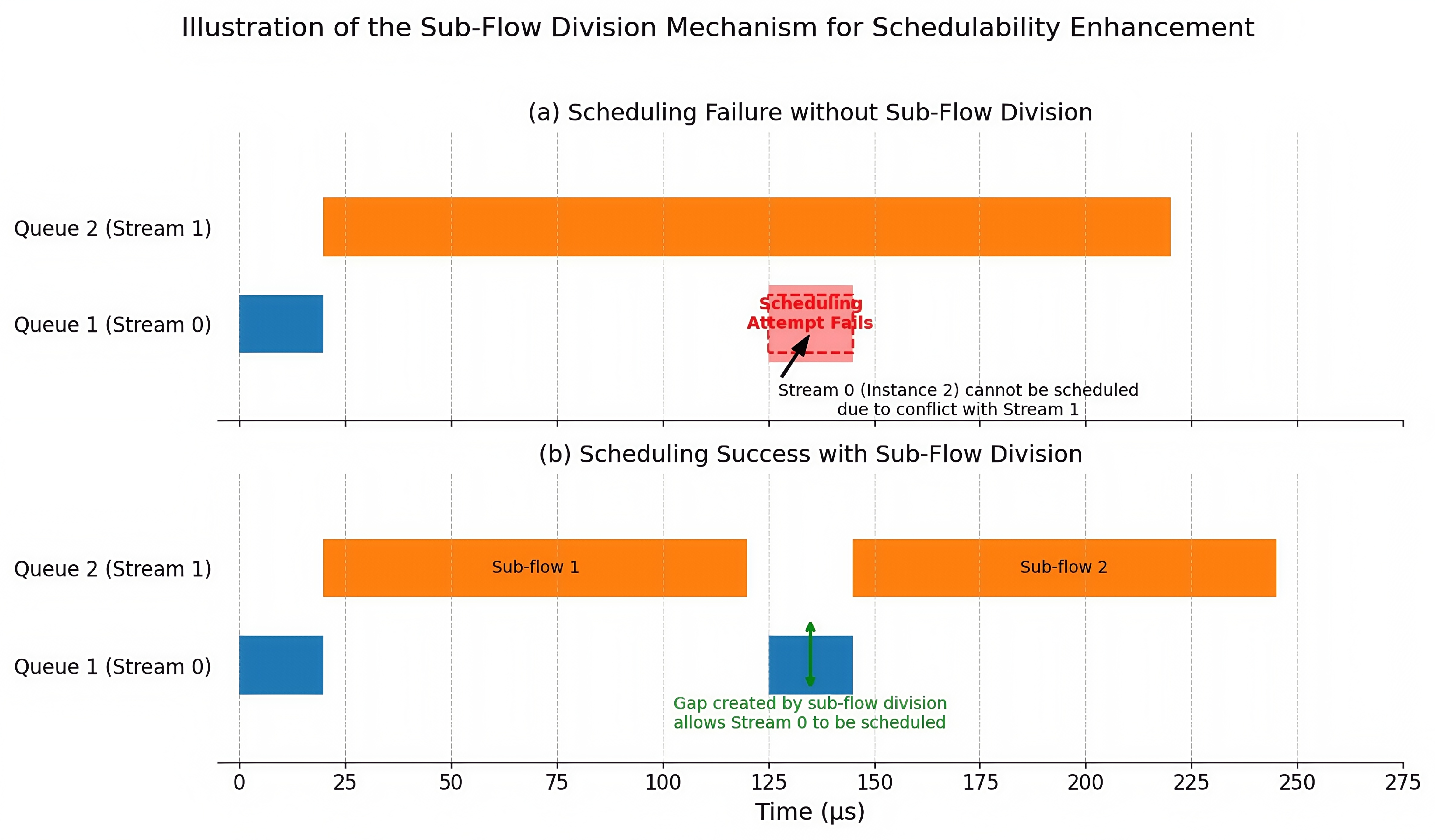
As shown in Figure 1, attempting to schedule these streams without sub-flow division leads to a failure. The long, contiguous transmission of Data Stream 1 occupies a critical time window, making it impossible for the scheduler to find a valid slot for Data Stream 0 to meet its deadline in a subsequent cycle. However, by activating the sub-flow division mechanism, the high-bandwidth Data Stream 1 is automatically segmented into smaller, more flexible sub-flows. This segmentation creates the necessary scheduling gaps in the timeline, allowing the deadline-critical stream to be successfully placed. This example clearly demonstrates how the integrated sub-flow division capability directly enhances the schedulability of complex stream sets, making it a vital component of the baseline algorithm.

Algorithm 1 Stream Preprocessing, Filtering, and Sub-Flow Division Parameter Calculation

Require: Set of all input data streams ${\mathcal{F}}_{all}=\{F_1,\cdots ,F_m\}$. Ensure: Hyperperiod $\mathcal{T}$; For each $F_i\in {\mathcal{S}}_{sched}$: Available time $A_i$, Sub-stream count $N_i$, Sub-stream times $\left\{a_{i,x}\right\}$. 1: ${\mathcal{S}}_{sched}\leftarrow \varnothing$. 2: ${\mathcal{P}}_{all\_periods}\leftarrow \varnothing$.            ▹ List to collect periods of all schedulable streams 3: for all each unique path $P_k$ present in ${\mathcal{F}}_{all}$ do 4:     ${\mathcal{S}}_{path}\leftarrow \{F_j\in {\mathcal{F}}_{all}\mid F_j\mathrm{uses}\mathrm{path}{P}_k\}$. 5:     while ${\mathcal{S}}_{path}\ne \varnothing$ do 6:         $U_{util}\leftarrow {\sum }_{F_j\in {\mathcal{S}}_{path}}(t_j/T_j)$.         ▹ Calculate path utilization, Equation (7) 7:         if $0<U_{util}<1$ then 8:            ${\mathcal{S}}_{sched}\leftarrow {\mathcal{S}}_{sched}\cup {\mathcal{S}}_{path}$. 9:            Add periods of streams in ${\mathcal{S}}_{path}$ to ${\mathcal{P}}_{all\_periods}$. 10:           break while.         ▹ Path is schedulable with current streams 11:        else 12:            $F_{remove}\leftarrow \mathrm{null}$. 13:            if streams in ${\mathcal{S}}_{path}$ have distinct $PC{P}_j$ then 14:                $F_{remove}\leftarrow$ stream in ${\mathcal{S}}_{path}$ with lowest $PC{P}_j$. 15:            else if $|{\mathcal{S}}_{path}|>0$ then 16:                $F_{remove}\leftarrow$ stream in ${\mathcal{S}}_{path}$ with largest $(t_j/T_j)$ ratio. 17:            if $F_{remove}\ne \mathrm{null}$ then 18:                ${\mathcal{S}}_{path}\leftarrow {\mathcal{S}}_{path}\setminus \left\{F_{remove}\right\}$.                 ▹ Cull stream 19:            else 20:                break while.         ▹ Cannot prune further or path empty 21: if ${\mathcal{S}}_{sched}=\varnothing$ then return Error: No schedulable streams found after filtering. 22: $\mathcal{T}\leftarrow \mathrm{lcm}\mathrm{of}\mathrm{unique}\mathrm{periods}\mathrm{in}{\mathcal{P}}_{all\_periods}$. 23: Sort ${\mathcal{S}}_{sched}$ into ${\mathcal{S}}_{ordered}=(F_{\left(1\right)},\cdots ,F_{\left(N_s\right)})$ by increasing period $T_{\left(i\right)}$. 24: Let $T_{first\_period}\leftarrow T_{\left(1\right)}$ (period of the first stream in sorted list). 25: for all $F_{\left(i\right)}=(L_{\left(i\right)},t_{\left(i\right)},T_{\left(i\right)},\cdots )\in {\mathcal{S}}_{ordered}$ (iterating $idx$ from 1 to $N_s$) do 26:     if $idx=1$ then 27:         $A_{\left(idx\right)}\leftarrow T_{\left(idx\right)}$. 28:     else 29:         $A_{\left(idx\right)}\leftarrow (1-{\sum }_{k=1}^{idx-1}(t_{\left(k\right)}/T_{\left(k\right)}))·T_{\left(idx\right)}$.   ▹ Calculate available time based on prior streams 30:     $N_{\left(idx\right)}\leftarrow 1$.                 ▹ Default to no sub-flow division 31:     if $A_{\left(idx\right)}>0\mathbf{and}{T}_{first\_period}>0\mathbf{and}{T}_{\left(idx\right)}>0$ then 32:         $avg\_substream\_slots\_in\_Ai\leftarrow \lceil T_{\left(idx\right)}/T_{first\_period}\rceil$.     ▹ Ratio of periods, effectively number of $T_{first\_period}$ intervals in $T_{\left(idx\right)}$ 33:             if $avg\_substream\_slots\_in\_Ai>0$ then 34:                $target\_substream\_duration\leftarrow A_{\left(idx\right)}/avg\_substream\_slots\_in\_Ai$.   ▹ Target duration for a sub-stream if $F_{\left(idx\right)}$ was to be divided based on $T_{first\_period}$’s scale 35:                if $target\_substream\_duration>0\mathbf{and}{t}_{\left(idx\right)}>target\_substream\_duration$ then       ▹ Only divide if original stream is longer than target sub-stream duration 36:                  $N_{\left(idx\right)}\leftarrow \lceil t_{\left(idx\right)}/target\_substream\_duration\rceil$. 37:     if $N_{\left(idx\right)}>1$ then            ▹ If sub-flow division is determined 38:         for all $x=1$ to $N_{\left(idx\right)}$ do 39:            if $x<N_{\left(idx\right)}$ then 40:                $a_{\left(idx\right),x}\leftarrow \lfloor t_{\left(idx\right)}/N_{\left(idx\right)}\rfloor$. 41:            else 42:                $a_{\left(idx\right),x}\leftarrow t_{\left(idx\right)}-(N_{\left(idx\right)}-1)·\lfloor t_{\left(idx\right)}/N_{\left(idx\right)}\rfloor$.      ▹ Last sub-stream takes remainder 43:     else                  ▹ No sub-flow division, $N_{\left(idx\right)}=1$ 44:         $a_{\left(idx\right),1}\leftarrow t_{\left(idx\right)}$. 45:     Store $A_{\left(idx\right)}$, $N_{\left(idx\right)}$, and $\left\{a_{\left(idx\right),x}\right\}$ for $F_{\left(i\right)}$. 46: return$\mathcal{T}$, and parameters ($A_i,N_i,\left\{a_{i,x}\right\}$) for $F_i\in {\mathcal{S}}_{sched}$.

2.4.2. Iterative Constraint Boundary Determination and GCL Generation via SMT Solver

Once the streams are prepared, the algorithm proceeds to determine the precise schedule start times ${\phi }_{i,j,\mu }$ (or ${\varphi }_{i,\mu }$ for undivided streams) that satisfy all constraints from Section 2.3. This is achieved using an iterative approach coupled with the Z3 SMT solver.

The core challenge lies in finding appropriate, yet tight, boundaries for operational constraints such as end-to-end latency, jitter, and inter-cycle start time deviations, as these directly impact schedulability and performance. The iterative process is as follows:

1.

Initial Strict Constraint Setting: The process begins by establishing the most stringent (i.e., performance-optimal) target values for latency and jitter. For each stream $F_i$, ${\mathrm{LatencyRequirements}}_i$ is initialized to its minimum possible value (sum of its total transmission time over the path, all propagation delays, and minimal switch processing times, effectively aiming for zero queuing delay). ${\mathrm{JitterRequirements}}_i$ is set to a near-zero value (e.g., 1 µs). The deadlines $D_i$ are taken as hard upper bounds from user input, and inter-cycle start time deviations ${\delta }_i$ are initially set to tight values.

2.

SMT Solver Invocation: With the current set of constraint boundaries, the Z3 SMT solver is invoked. The solver attempts to find a satisfying assignment for all ${\phi }_{i,j,\mu }$ variables that meets all mathematical constraints defined in Section 2.3.

3.

Adaptive Constraint Relaxation: If the SMT solver reports that the problem is unsatisfiable with the current constraint boundaries, the algorithm systematically relaxes the ${\mathrm{LatencyRequirements}}_i$ and ${\mathrm{JitterRequirements}}_i$. This relaxation is typically performed iteratively:

• Relaxation prioritizes lower-priority streams first.
• The values are increased by small increments.
• After each relaxation step, the SMT solver is invoked again (Step 2).

User-defined deadlines $D_i$ are generally treated as hard constraints and are not relaxed unless all other avenues fail and the application permits.

4.

Convergence and GCL Finalization: This iterative loop of solving and relaxing constraints continues until the SMT solver finds a feasible solution. The objective is to converge to the “tightest” possible set of latency and jitter values for which the entire stream set ${\mathcal{S}}_{sched}$ is schedulable. Once a feasible set of start times ${\phi }_{i,j,\mu }$ is determined, the GCL is constructed. For each sub-stream $f_{i,j}$, its transmission window in each cycle instance $\mu$ is $[{\phi }_{i,j,\mu },{\phi }_{i,j,\mu }+a_{i,j}]$. These time windows, along with the $PC{P}_i$ of the corresponding original stream $F_i$, define the GCL entries. Each entry specifies the opening and closing times of the transmission gate for the queue associated with $PC{P}_i$ on the relevant TSN switch output ports along path $P_i$.

This SMT-based iterative approach allows for a robust search for a feasible GCL that adheres to complex timing constraints while attempting to optimize for low latency and jitter. If sub-flows were created during preprocessing, they are treated as individual scheduling entities during this GCL computation phase; their reassembly into the original data stream is assumed to occur at the receiving end-station.

2.5. Optimization: Scheduling Computation Acceleration Algorithm

While the SMT-based approach detailed in Section 2.4 provides a robust method for finding feasible GCLs, its computational complexity can become a bottleneck for scenarios involving a very large number of data streams or requiring rapid GCL recalculation, which are characteristic of complex autonomous driving systems. Handling large-scale periodic scheduling is a significant challenge in TSN [28], and to this end, a scheduling computation acceleration algorithm is proposed. This algorithm employs a heuristic-based, linear-time local search strategy designed to significantly reduce the time required to compute the GCL, while still aiming to satisfy the critical timing constraints of time-sensitive traffic.

The acceleration algorithm operates based on the following core principles and steps:

1.

Time Slot Discretization: The entire hyperperiod $\mathcal{T}$ (obtained from Algorithm 1) is discretized into a sequence of fine-grained, elementary time slots. A typical slot duration is 1 µs, chosen based on the assumption that underlying TSN switch hardware can support GCL operations at this level of temporal granularity and that per-stream switch processing overheads are generally within this magnitude. Each stream (or sub-stream) transmission will occupy an integer number of these elementary slots.

2.

Initial Search Phase-Prioritized Greedy Placement: This phase aims to quickly place a majority of streams into the discretized timeline with minimal conflicts.

• Two-Level Sorting Strategy: The set of schedulable streams ${\mathcal{S}}_{sched}$ (or their constituent sub-streams if $N_i>1$ from Algorithm 1) are first sorted according to a two-level criterion to prioritize their placement.

  (i)

  Primary Sort: Streams are sorted by the earliest start time of their respective cycle instances within the hyperperiod, in ascending order. This prioritizes streams that become available for transmission sooner.

  (ii)

  Secondary Sort: Streams with the same primary sort key (i.e., same cycle start time) are then sorted by their transmission time ($t_i$ or $a_{i,x}$), in ascending order (shortest transmission time first). Placing shorter streams first tends to leave larger contiguous blocks of time slots, potentially improving schedulability for subsequent, longer streams.

• Sequential Greedy Placement: Following the sorted order, the algorithm attempts to place each stream (or sub-stream) into the earliest available sequence of unoccupied time slots on the timeline. The placement must respect the stream’s cycle start time within the current instance of its period being scheduled in the hyperperiod and all applicable constraints from Section 2.3 that can be checked at this stage (e.g., deadline, no-conflict with already placed streams).

3.

Final Search Phase-Conflict Resolution via Local Search and Limited Backtracking: It is possible that during the initial greedy placement, some streams cannot be placed without violating constraints. This phase attempts to resolve such conflicts:

• Direct Alternative Placement: For an unplaced stream, the algorithm first searches for an alternative valid placement in a later available time slot that still satisfies all its constraints (especially its deadline $D_i$).
• Limited Backtracking and Local Search: If no direct alternative slot is available due to occupation by previously placed streams, a limited backtracking or local search mechanism is triggered. This search prioritizes relocating already-placed, lower-priority streams to resolve conflicts, with the constraint of displacing only one conflicting stream at a time. If the displaced stream can be successfully rescheduled to another valid slot without inducing further conflicts, the relocation is accepted, enabling placement of the current stream. This constrained approach prevents degeneration into exhaustive search, thereby preserving the algorithm’s near-linear time complexity.

4.

GCL Output: Once all streams that can be successfully placed by this heuristic are scheduled into time slots, their determined start and end slot indices, along with their respective $PC{P}_i$ values, directly translate into the GCL entries for the TSN switches.

It is important to emphasize that as a heuristic method, the proposed acceleration algorithm does not guarantee finding a feasible schedule, even if one exists. Its design prioritizes computational speed over completeness, making it particularly suitable for dynamic environments with limited computational resources for scheduling tasks. In scenarios where the network is highly congested or constraints are extremely tight, the greedy placement and limited backtracking may fail to find a valid GCL. In such cases, the algorithm would report a failure, and a more exhaustive method, such as the SMT-based baseline algorithm, would be required. The primary value of the acceleration algorithm lies in its ability to quickly find high-quality, feasible schedules for the vast majority of practical, non-pathological scenarios.

The conceptual pseudo-code for this algorithm is outlined in Algorithm 2.

Algorithm 2 Scheduling Computation Acceleration Heuristic

Require: Set of schedulable streams/sub-streams ${\mathcal{S}}^{\prime }=\{s_1,\cdots ,s_N\}$ (output from Algorithm 1, each $s_k$ has attributes like $i{d}_k, {cycle\_start\_offsets}_k, {\mathrm{duration}}_k, {\mathrm{deadline}}_k, {\mathrm{period}}_k, PC{P}_k$). Hyperperiod $\mathcal{T}$. Constraints C (from Section 2.3). Ensure: Gate Control List (GCL). 1: Initialize GCL timeline for hyperperiod $\mathcal{T}$ with all 1 µs slots marked as AVAILABLE. 2: Sort ${\mathcal{S}}^{\prime }$ using the two-level sorting strategy: (1) by earliest cycle start time instance in $\mathcal{T}$, then (2) by stream duration (ascending). 3: Let $PlacedInstances\leftarrow \varnothing$.      ▹ A set to track successfully placed stream instances 4: for all $s_k\in {\mathcal{S}}^{\prime }$ (in sorted order) do 5:     for all cycle instance $\mu$ of $s_k$ within $\mathcal{T}$ do 6:         $is\_placed\_this\_instance\leftarrow false$. 7:         Determine earliest valid start slot $slo{t}_{start}$ for $s_k$ in instance $\mu$. 8:         $current\_attempt\_slot\leftarrow slo{t}_{start}$. 9:         while $current\_attempt\_slot+{\mathrm{duration}}_k\le {deadline\_for\_instance}_{\mu }\left(s_k\right)$ and not $is\_placed\_this\_instance$ do 10:            if Slots from $current\_attempt\_slot$ to $current\_attempt\_slot+{\mathrm{duration}}_k-1$ are AVAILABLE and placement satisfies C then 11:                Mark slots as OCCUPIED by instance $(s_k,\mu )$ in GCL timeline. Add $(s_k,\mu )$ to $PlacedInstances$. 12:                $is\_placed\_this\_instance\leftarrow true$. 13:            else 14:                  $current\_attempt\_slot\leftarrow current\_attempt\_slot+1$.         ▹ Try next µs slot 15:         if not $is\_placed\_this\_instance$ then 16:            $ConflictingInstances\leftarrow$ Identify instances in $PlacedInstances$ that occupy desired slots for $(s_k,\mu )$. 17:            Sort $ConflictingInstances$ by priority (ascending, i.e., lower PCP first). 18:            for all instance $s_{conflict}$ in $ConflictingInstances$ do 19:                Temporarily remove $s_{conflict}$ from GCL timeline and $PlacedInstances$. 20:                if can place $(s_k,\mu )$ in the now-available slot then 21:                    Place $(s_k,\mu )$ in GCL timeline. Add $(s_k,\mu )$ to $PlacedInstances$. 22:                    if can find a new valid slot for $s_{conflict}$ then 23:                        Place $s_{conflict}$ in its new slot. Add $s_{conflict}$ back to $PlacedInstances$. 24:                        $is\_placed\_this\_instance\leftarrow true$. 25:                        break         ▹ Conflict resolved, exit inner For loop 26:                    else 27:                        Revert: Place $s_{conflict}$ back, remove $(s_k,\mu )$ from GCL timeline and $PlacedInstances$. 28:                else 29:                    Revert: Place $s_{conflict}$ back to its original slot. 30:         if not $is\_placed\_this\_instance$ then 31:            Log instance $(s_k,\mu )$ as unplaced by this heuristic. 32: Construct final GCL data structure from the GCL timeline. 33: return GCL.

3. Model Implementation

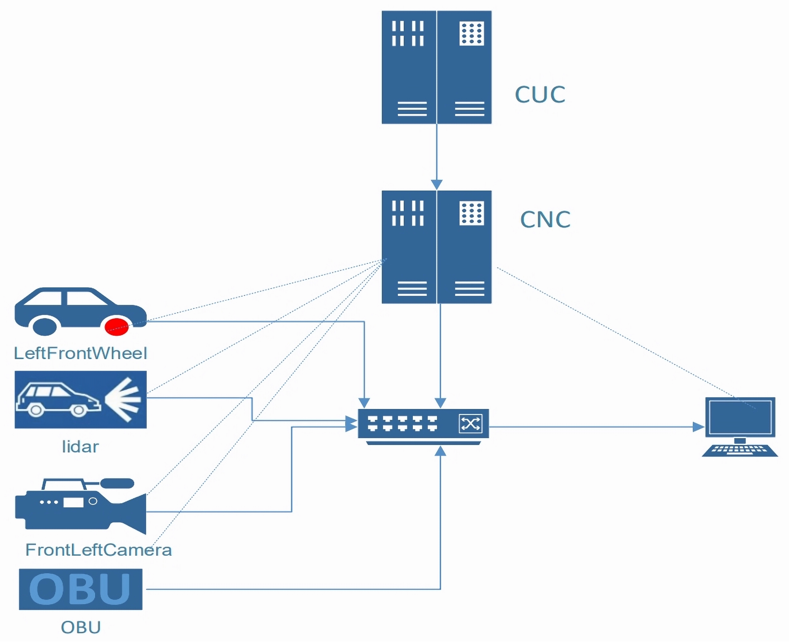
This section details the implementation of the proposed Time-Sensitive Networking (TSN) scheduling system within a simulated in-vehicle network environment. The implementation adheres to the centralized configuration model defined by IEEE 802.1Qcc [16], encompassing both a control plane for scheduling decisions and a data plane for deterministic packet transmission. The overall architecture, illustrating the interaction between these components and the end devices, is depicted in Figure 2.

3.1. Control Plane Implementation: CUC and CNC

The control plane is responsible for collecting stream requirements, computing the transmission schedule (GCL), and configuring the network devices. It consists of two primary logical entities: the Centralized User Configuration (CUC) and the Centralized Network Configuration (CNC).

• Centralized User Configuration (CUC): The CUC serves as the interface for specifying the requirements of various data streams, particularly the Time-Triggered (TT) streams which demand deterministic transmission. For each TT stream $F_i$, users (or higher-level application planners) provide its characteristic parameters as defined in Section 2 (Table 1). These include its length $L_i$ (or transmission time $t_i$), period $T_i$, deadline $D_i$, intended transmission path $P_i$ through the network, and its Priority Code Point ($PC{P}_i$).
• Centralized Network Configuration (CNC): The CNC is the core intelligence of the control plane. It receives the stream requirements gathered from the CUC and the network topology information. The CNC then executes the scheduling logic to generate the GCL. In this work, the CNC implements the Baseline Scheduling Algorithm with Sub-Flow Division (detailed in Section 2.4) to compute the GCL. This involves stream preprocessing and filtering, sub-flow division for high-bandwidth streams (using Algorithm 1), iterative determination of constraint boundaries, and finally, invoking the Z3 SMT solver to compute the precise start times (${\phi }_{i,j,\mu }$ or ${\varphi }_{i,\mu }$) for all scheduled transmissions. Alternatively, for scenarios requiring faster computation, the CNC can employ the Scheduling Computation Acceleration Algorithm (detailed in Section 2.5). Once the GCL is computed, the CNC is responsible for translating this schedule into a format understood by the TSN switches and distributing it to the respective switches in the data plane to configure their gate control mechanisms.

3.2. Data Plane Implementation: TSN Devices and Switches

The data plane comprises the TSN end-devices (sensors, actuators, ECUs) that generate and consume TT streams, and the TSN switches that forward these streams according to the GCL.

• TSN End-Devices: These devices serve as the sources and sinks for data streams. As depicted in Figure 2, examples include wheel speed sensors (LeftFrontWheel), LiDAR units, cameras (FrontLeftCamera), and On-Board Units (OBUs). They are responsible for packetizing data, assigning PCP values, and transmitting frames at their designated cycle start times, potentially after performing sub-flow segmentation if dictated by the CNC’s scheduling parameters ($N_i>1$). Receiving devices are responsible for reassembling sub-flows if applicable.
• TSN Switches: The TSN switches are the core enablers of deterministic forwarding in the data plane. Each switch port is equipped with multiple priority queues and a Time-Aware Shaper (TAS) mechanism. Upon receiving the GCL from the CNC, the TAS in each switch configures its egress queue gates to open and close precisely according to the scheduled time intervals for each $PC{P}_i$. This ensures that frames from different streams are forwarded in a conflict-free manner, adhering to the computed schedule and minimizing queuing delays for TT traffic.

The operational flow for scheduling a set of TT streams is as follows. The CNC gathers all stream requests $F_i$ via the CUC. It first executes the preprocessing and filtering steps of Algorithm 1 to determine the set of schedulable streams ${\mathcal{S}}_{sched}$ and their sub-flow parameters. Then, using either the SMT-based iterative approach or the acceleration heuristic, it computes the GCL that satisfies all constraints defined in Section 2.3. This GCL is then deployed to the TSN switches. When multiple data streams are assigned the same priority level and are eligible for transmission within overlapping GCL-defined open windows (a situation ideally minimized by a precise GCL), the switch typically processes them based on a First-Come-First-Served (FCFS) principle within that priority queue during that window.

4. Experimental Results

This section presents a comprehensive evaluation of the proposed TSN scheduling algorithms. We validate their performance through simulations using the OMNeT++ platform and through experiments on a real-world hardware testbed, using the demanding in-vehicle network scenario as a representative use case for real-time systems. The evaluations focus on key metrics such as end-to-end latency, jitter, schedulability, and GCL computation time.

4.1. Experimental Setup

To thoroughly evaluate the proposed Time-Sensitive Networking (TSN) scheduling algorithms, a combination of simulation-based studies and experiments on a physical testbed were conducted. This dual approach allows for the assessment of algorithm performance under controlled, reproducible conditions as well as validation in a more realistic hardware environment.

4.1.1. Simulation Environment

The simulation experiments were primarily conducted using the OMNeT++ discrete event simulator, version 6.0.1, coupled with the INET framework, version 4.6. The INET framework’s TSN functionalities, which were significantly enhanced starting from its version 4.4, provided the necessary modules for modeling TSN switches, end-stations, and protocols. This particular TSN model within INET was co-developed by the OMNeT++ maintainers and automotive industry partners, ensuring its relevance and capability to simulate critical features pertinent to in-vehicle networking scenarios.

A cornerstone of Time-Aware Shaping (TAS) is precise time synchronization across all network nodes, typically achieved via protocols like gPTP (IEEE 802.1AS). This shared sense of time is fundamental to the offline GCL scheduling paradigm investigated in this paper, although alternative asynchronous approaches also exist [29]. The gPTP implementation within OMNeT++, whose modeling considerations are discussed in works like [30], demonstrated consistent nanosecond-level synchronization accuracy among simulated nodes throughout the experiments.

All simulations were executed on a host machine equipped with an 11th Generation Intel(R) Core(TM) i7-11800H processor (Intel Corporation, Santa Clara, CA, USA) and an NVIDIA RTX 3060 Laptop GPU (NVIDIA Corporation, Santa Clara, CA, USA), running a Windows 10 operating system. Unless specified otherwise for particular experiments, the simulated in-vehicle network architecture corresponded to the centralized model previously depicted in Figure 2, featuring a Centralized Network Configuration (CNC) entity responsible for GCL computation and distribution.

4.1.2. Real-World Testbed Environment

To validate the algorithms in a physical setting and observe their behavior with actual hardware, a real-world TSN testbed was constructed. This approach aligns with current research practices aimed at validating TSN solutions on physical automotive Ethernet testbeds [31]. The testbed utilized the ZIGGO platform, which includes ZIGGO TSN-compliant switches and the ZIGGO TSNPerf software  tool for traffic generation, network configuration, and performance analysis. The software, which does not have formal version releases, was obtained from the official GitHub repository, and the version used in this study corresponds to the state of the repository as of April 2024.

The key hardware components of the testbed were:

• FPGA Development Boards: Xilinx Zynq-series FPGA boards were employed to function as both TSN switches and end-nodes (traffic sources and sinks). These boards were flashed with custom TSN-capable firmware developed for the ZIGGO platform, enabling features like Time-Aware Shaping and gPTP synchronization.
• Host Computers: Two host computers, with specifications similar to the simulation host (11th Gen Intel(R) Core(TM) i7-11800H, NVIDIA RTX 3060, running Windows 10), were used for overall testbed control. Their roles included configuring the FPGA-based TSN devices, deploying computed Gate Control Lists (GCLs), initiating and monitoring traffic flows using TSNPerf, and collecting experimental data.

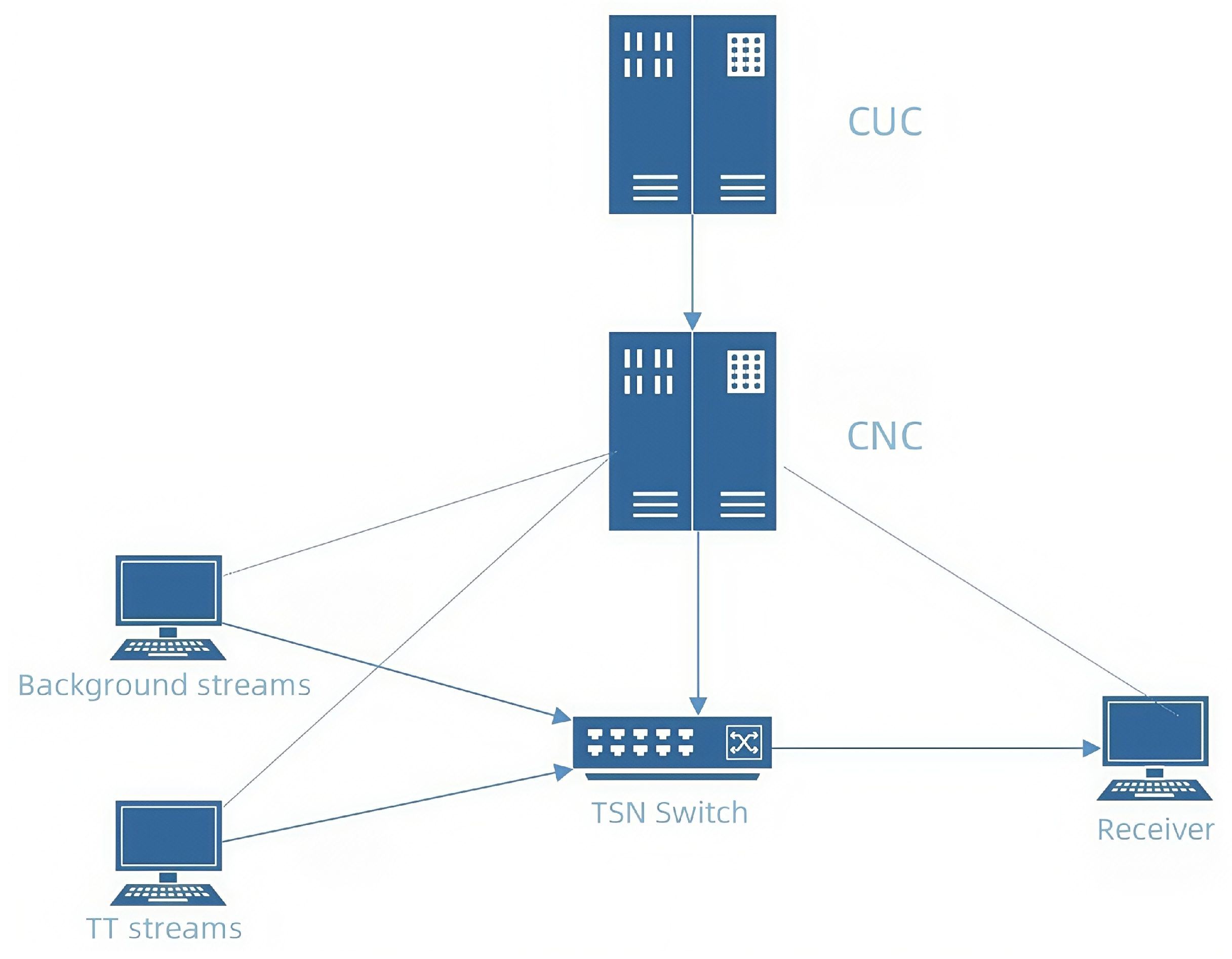
Configuration of the FPGA boards, including setting parameters such as hostnames, IP addresses, and MAC addresses, was performed using MobaXterm (Version 24.0, Mobatek, Montpellier, France) via serial port connections. Software components, including GCL files and traffic profiles, were transferred to the nodes securely using the Secure Shell (SSH) protocol [32]. The general network topology for the real-world experiments, illustrating the interconnection of emulated CUC/CNC components, traffic senders, the TSN switch, and receiver nodes, is shown in Figure 3.

In the real-world testbed, precise time synchronization was equally critical. The CaaS-Switch component within the ZIGGO platform was configured to act as the gPTP master clock. All other TSNPerf nodes operated as gPTP slaves, ensuring that all transmissions and GCL operations were coordinated within a single, precisely synchronized time domain. This setup allowed for the direct application and observation of the GCLs generated by the proposed scheduling algorithms in a physical network.

4.2. Performance Evaluation: Latency and Jitter for In-Vehicle Traffic

This set of experiments evaluates the baseline scheduling algorithm’s ability to achieve low-latency and low-jitter deterministic transmission for a realistic in-vehicle Time-Triggered (TT) traffic scenario. The TT stream data used in these simulations was based on specifications from an automotive manufacturer, representing typical critical data flows such as sensor readings and control commands. To simulate a more realistic mixed-criticality network environment, periodic best-effort (BE) background traffic with a low priority (PCP 0) was also transmitted concurrently with the TT streams.

The specific characteristics and constraints of the TT streams are detailed in

Table 3. Time-triggered (TT) stream characteristics and constraints for the in-vehicle traffic scenario.

Data Type	Priority (PCP:0–7)	Send Delay (µs)	Cycle Period (µs)	Deadline (µs)	Inter-Cycle Send Offset (µs)	E2E Latency Target (µs)	Jitter Target (µs)
LeftFrontWheel	6	10	500	11	0	11	0
Lidar	5	26	250	38	0	27	0
FrontLeftCamera	4	120	250	187	0	122	0
OBU	3	26	125	89	24	27	0

. The Gate Control Lists (GCLs) for this scenario were generated using our baseline scheduling algorithm (as described in Section 2.4) and subsequently deployed to the simulated TSN switches in OMNeT++. The deployment process involved setting the precise send offsets and time slice durations for each queue gate via the OMNeT++ configuration path: *switch.eth[*].macLayer.queue.transmissionGate[*].

To verify the correct execution of the generated GCL, Figure 4 presents a Gantt chart that overlays the planned schedule with the actual transmission events recorded during the simulation. The colored bars represent the “Planned GCL Open-Gate Windows”, which are the time intervals during which the transmission gate for a specific priority queue is scheduled to be open. The black ‘x’ markers indicate the “Actual Packet Transmission Events”, showing the precise timestamps when packets were transmitted from the switch’s egress port.

As depicted in Figure 4, every actual packet transmission event falls perfectly within its corresponding planned open-gate window. This provides strong visual evidence that the GCL was correctly computed and deployed, and that the TSN switch adhered to the schedule with high fidelity, thus achieving deterministic transmission. The effect of this precise scheduling is further reflected in the switch’s queue lengths, shown in Figure 5. The queue lengths for the TT streams remained minimal and exhibited stable, periodic behavior, confirming that queuing delay—the primary variable delay component in a switched network—was effectively eliminated by the pre-scheduled gate openings.

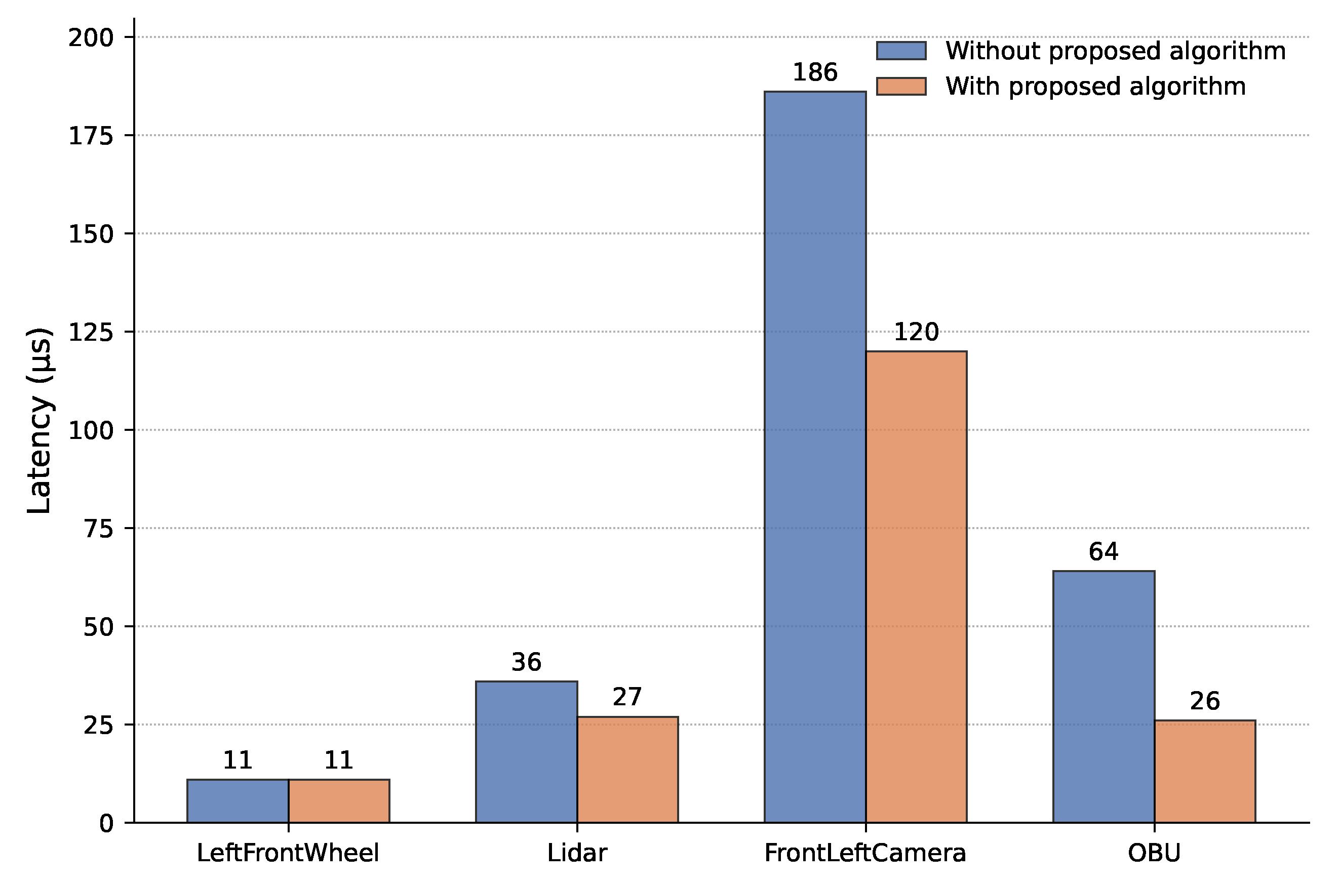
Finally, the overall performance impact is quantified in Figure 6, which compares the total end-to-end latency of the TT streams when scheduled by our proposed algorithm versus a standard Strict Priority (SP) scheduling algorithm. With our algorithm, the portion of the delay attributable to propagation, processing, and queuing was consistently less than 1 µs for all TT streams. This resulted in a maximum reduction in total end-to-end latency of up to 59% for certain streams compared to SP scheduling. Furthermore, the maximum observed deviation in end-to-end latency (jitter) for streams scheduled by our algorithm was controlled at the nanosecond level, highlighting a significant improvement in transmission predictability. A 100% scheduling success rate was achieved for all TT streams in this scenario, even with their cumulative bandwidth occupancy exceeding 81%.

This demonstrated level of deterministic performance not only fulfills the stringent safety requirements of automotive applications but is also directly applicable to other demanding Future Internet domains, such as factory floor automation and remote tele-robotics.

4.3. Performance Evaluation with Large-Scale Traffic

To assess the scalability and performance of the proposed scheduling algorithm under more demanding network conditions, experiments were conducted with a significantly larger set of 100 data streams. These streams were randomly generated to simulate a high-load, complex traffic scenario with the following characteristics:

• Cycle periods were randomly chosen from the set {125 µs, 250 µs, 500 µs, 1000 µs}.
• Transmission times ranged from 2 to 5 µs.
• Priorities (PCP values) were randomly assigned integers between 2 and 5 (inclusive).
• The parameters were set to ensure that the total bandwidth utilization by these streams was above 70%.

During the GCL calculation for this scenario, an additional time margin of 1 µs was reserved for each stream to account for factors such as propagation delay and the TSN switch’s internal processing time; this value was empirically determined through prior measurements.

It is noted that the selected cycle periods for the large-scale traffic generation (125, 250, 500, 1000 µs) form a harmonic set, resulting in a simple hyperperiod. This choice was made to reflect common scenarios in embedded and automotive systems where task periods are often assigned as multiples of a base clock rate. The practice of assigning harmonic periods is a well-studied topic in real-time systems, as it can simplify schedulability analysis and improve resource utilization [33]. While this may simplify the scheduling problem compared to non-harmonic period sets, it provides a realistic and relevant baseline for comparing the computational efficiency of different algorithms. The performance evaluation with non-harmonic periods, which can lead to a significantly larger hyperperiod and a more fragmented scheduling problem, remains an important direction for future work.

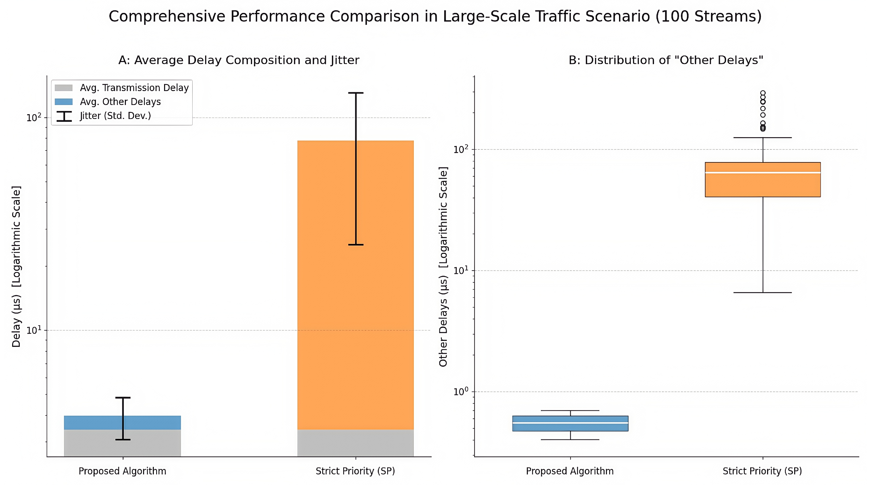
A comprehensive comparison between our proposed algorithm and a standard Strict Priority (SP) scheduling algorithm is presented in Figure 7. This composite figure provides two perspectives on performance: subplot A illustrates the average delay composition and jitter, while subplot B details the distribution of the variable delay component.

The analysis of Figure 7 reveals several key findings:

1.

Average Delay Composition (Figure 7A): The stacked bar chart clearly shows that while the average Transmission Delay (gray portion) is identical for both algorithms, as it is an input parameter, the average “Other Delays” (colored portion) differ dramatically. For the proposed algorithm, this component is negligibly small, whereas for SP scheduling, it constitutes the vast majority of the total delay, with an average value of approximately 57.19 µs.

2.

Jitter Comparison (Figure 7A): The error bars, representing the standard deviation of the total delay across all streams, provide a quantitative measure of jitter. The error bar for the proposed algorithm is extremely short, indicating highly consistent and predictable latency. In contrast, the large error bar for the SP algorithm reflects significant jitter, with delay variations reaching up to 300 µs for some streams.

3.

Distribution of “Other Delays” (Figure 7B): The box plot provides a deeper look into the distribution of the variable delay component. For the proposed algorithm, the entire distribution (the blue box) is tightly clustered in the sub-microsecond range (400–700 ns), confirming extremely low and stable queuing delays for all 100 streams. Conversely, the box plot for SP scheduling (orange) shows a much higher median delay and a wide interquartile range, along with several outliers, visually confirming its high latency and poor predictability. The measured end-to-end jitter for all streams under our algorithm was less than 400 ns.

In conclusion, these results confirm that even with a large number of data streams and high network utilization, the proposed scheduling algorithm successfully maintains low-latency, low-jitter deterministic transmission. It significantly outperforms standard SP scheduling by virtually eliminating queuing delay and providing highly consistent and predictable performance. This ability to efficiently schedule hundreds of concurrent streams is a key enabler for deploying complex and scalable real-time IoT systems.

4.4. Analysis of GCL Computation Time

This subsection evaluates the computational efficiency of the proposed Scheduling Computation Acceleration Algorithm (detailed in Section 2.5). Its GCL computation time is compared against several other scheduling approaches to demonstrate its scalability and suitability for large-scale in-vehicle networks.

For this evaluation, TSN traffic flow sets were randomly generated, with the number of data streams varying from 25 to 200. For each set, streams were assigned random parameters; cycle periods were selected from the set {125 µs, 250 µs, 500 µs, 1000 µs}, priorities (PCP values) were assigned from 0 to 7, and transmission times were configured to ensure the total network bandwidth utilization exceeded 70%.

The significant variation in schedule quality and runtime among different algorithms necessitates such empirical comparisons, as demonstrated in recent benchmarking studies [34]. The compared methods in our study include an exact Integer Linear Programming (ILP) formulation solved with Z3, metaheuristics like a Genetic Algorithm and Tabu Search, a Domain-Specific Knowledge (DSK)-based heuristic, a DeepScheduler using deep learning, and a simple Random greedy placement algorithm.

The average GCL computation times across multiple runs are presented in

Table 4. Average GCL computation times (seconds) for different algorithms and varying numbers of data flows.

Algorithm	25 Flows	50 Flows	75 Flows	100 Flows	125 Flows	150 Flows	175 Flows	200 Flows
Random	0.5	0.9	1	2	3	5	6	8
Genetic	0.5	0.9	1	1.15	8	20	60	70
Tabu	0.05	0.2	6	30	90	500	800	2000
DSK	9	19	20	30	40	50	60	70
ILP (Z3)	500	2000	3000	4000	>3600	>3600	>3600	>3600
DeepScheduler	0.8	1.5	2	3	4	6	7	9
Proposed Acceleration Heuristic	0.107	0.206	0.355	0.488	0.617	0.744	0.78	1.06

.

The results in Table 4 clearly demonstrate the scalability challenges inherent in TSN scheduling. The exact ILP method, while optimal, exhibits exponential time complexity, becoming computationally prohibitive (requiring over an hour) for 100 or more data streams. In contrast, most heuristic and learning-based approaches show approximately linear time growth.

Notably, our proposed acceleration algorithm consistently outperforms the other scalable methods. This superior efficiency is attributed to its two-level sorting heuristic, which effectively prunes the search space and minimizes the need for extensive backtracking during the placement process. For a demanding scenario with 200 data flows, our algorithm computes the GCL in an average of approximately 1.06 s, confirming its suitability for large-scale networking applications. This sub-second computation time makes the framework viable for dynamic real-time systems where network schedules may need to be adapted or recalculated rapidly in response to changing conditions.

4.5. Real-World Experimentation and Validation

To corroborate the simulation findings and validate the practical applicability of the proposed scheduling approach, experiments were conducted on the real-world TSN testbed described in Section 4.1.2, utilizing the ZIGGO platform.

In a representative experiment, the Gate Control List (GCL) generated by our algorithm was deployed to the FPGA-based TSN switch. The test scenario involved a high-rate Time-Triggered (TT) stream, configured to transmit 1500-byte packets, and lower-priority background traffic, all scheduled within a 33 ms hyperperiod. The GCL allocated specific, protected time slots for the TT stream to ensure its deterministic delivery.

The key performance metrics from this real-world experiment are summarized in Figure 8. Subplot (a) confirms that the prerequisite of precise time synchronization was met, while subplot (b) presents the end-to-end latency performance of the TT stream.

The analysis of the real-world results provides strong validation for our proposed scheduling algorithm:

1.

Time Synchronization Efficacy: As shown in Figure 8a, the gPTP time synchronization mechanism functioned effectively on the hardware testbed. The plot illustrates that the clock offset between nodes rapidly converged from an initial larger value and remained stable within a tight bound of approximately ±50 ns, establishing the high-precision, shared sense of time required for TAS execution.

2.

Deterministic Latency and Low Jitter: Figure 8b presents the latency distribution for thousands of received TT packets. The histogram reveals an extremely narrow and sharp peak, indicating highly consistent end-to-end latency. The data, extracted and analyzed from the testbed logs, shows a mean latency of approximately 26.24 µs. Critically, the variation around this mean (the jitter) was exceptionally low, with the vast majority of packets arriving within a 100 ns window.

The results from the physical testbed align with the simulation findings. They confirm that the GCLs generated by our algorithm, when deployed on real TSN hardware, successfully enable the deterministic transmission of time-critical data streams with low, predictable latency and extremely low jitter, validating the practical effectiveness of our approach. This successful validation on physical hardware provides strong confidence in the applicability of our scheduling framework for real-world deployments of future internet technologies.

5. Conclusions

The primary contributions of this work are twofold. First, we proposed a novel baseline TAS scheduling algorithm that integrates an innovative sub-flow division mechanism. This mechanism enhances schedulability by intelligently segmenting high-bandwidth data streams that would otherwise cause scheduling conflicts, a common issue in mixed-criticality automotive environments. The algorithm employs an iterative, SMT-solver-based approach to determine tight constraint boundaries, aiming to generate GCLs optimized for low latency and jitter. Second, to address the computational demands of large-scale scenarios, we introduced a distinct scheduling computation acceleration algorithm. This algorithm utilizes a linear-time heuristic strategy, including a two-level sorting method and local search, to drastically reduce GCL computation time without significant performance degradation.

A comprehensive experimental evaluation, conducted through both simulations and on a real-world hardware testbed, validated the effectiveness of the proposed framework. The key findings demonstrate that:

• For realistic in-vehicle traffic, the proposed scheduling algorithm achieved a reduction in end-to-end latency of up to 59% compared to standard Strict Priority scheduling, with jitter controlled at the nanosecond level. Queuing delay was virtually eliminated by the precise GCL scheduling.
• The algorithm successfully scales to larger networks, maintaining low latency (less than 700 ns above transmission delay) and low jitter (less than 400 ns) for scenarios with 100 or more data streams.
• The scheduling computation acceleration algorithm proved highly efficient, capable of computing a GCL for 200 data streams in approximately 1.06 s, a significant improvement over traditional methods like ILP, which become computationally intractable for large stream sets.
• Real-world experiments on a ZIGGO/FPGA testbed confirmed the practical applicability of our approach, demonstrating deterministic packet reception with low, stable latency (a mean of approx. 26.24 µs) and extremely low jitter (within a 100 ns range) on physical hardware.

In summary, this paper presents a practical and scalable solution for TAS-based scheduling in autonomous in-vehicle networks. By addressing both schedulability for complex traffic mixes and the computational efficiency for large-scale systems, this work contributes to the advancement of robust and reliable communication backbones essential for the future of autonomous driving.

Future work will focus on extending these contributions. Key directions include (1) validating the algorithm in more complex, real-world in-vehicle network environments with an even greater diversity of nodes and traffic patterns; (2) optimizing the algorithms to handle dynamic data stream requirements, where traffic characteristics may change during operation; (3) exploring the integration and interplay of the proposed TAS scheduling algorithm with other TSN mechanisms, such as Cyclic Queuing and Forwarding (CQF); and (4) addressing the practical challenges of interoperability between TSN devices from different manufacturers.

References

- Khalid, A.; Kirisci, P.; Khan, Z.H.; Thoben, K.D. Security framework for industrial collaborative robotic cyber-physical systems. Comput. Ind. 2018, 97, 132–145. [Google Scholar] [CrossRef]
- IEEE Std 802.1Q-2022; IEEE Standard for Local and Metropolitan Area Networks—Bridges and Bridged Networks. IEEE: Piscataway, NJ, USA, 2022.
- Zhang, T.; Wang, G.; Xue, C.; Wang, J.; Nixon, M.; Han, S. Time-Sensitive Networking (TSN) for Industrial Automation: Current Advances and Future Directions. ACM Comput. Surv. 2024, 57, 1–38. [Google Scholar] [CrossRef]
- Peng, Y.; Shi, B.; Jiang, T.; Tu, X.; Xu, D.; Hua, K. A Survey on In-Vehicle Time-Sensitive Networking. IEEE Internet Things J. 2023, 10, 14375–14396. [Google Scholar] [CrossRef]
- Pal, B.; Khaiyum, S.; Kumaraswamy, Y.S. Recent advances in Software, Sensors and Computation Platforms Used in Autonomous Vehicles, A Survey. Int. J. Res. Anal. Rev. 2019, 6, 383–399. [Google Scholar]
- Zhou, Z.; Lee, J.; Berger, M.S.; Scharbarg, J.L.; Zinner, T.; Korf, F. Simulating TSN traffic scheduling and shaping for future automotive Ethernet. J. Commun. Netw. 2021, 23, 53–62. [Google Scholar] [CrossRef]
- Minaeva, A.; Akesson, B.; Hanzálek, Z.; Tovar, E. Time-triggered co-scheduling of computation and communication with jitter requirements. IEEE Trans. Comput. 2017, 67, 115–129. [Google Scholar] [CrossRef]
- Deng, L.; Zeng, G.; Kurachi, R.; Takada, H.; Xiao, X.; Li, R.; Xie, G. Enhanced Real-Time Scheduling of AVB Flows in Time-Sensitive Networking. ACM Trans. Des. Autom. Electron. Syst. 2024, 29, 1–26. [Google Scholar] [CrossRef]
- Nie, H.; Su, Y.; Zhao, W.; Mu, J. Hybrid Traffic Scheduling in Time-Sensitive Networking for the Support of Automotive Applications. IET Commun. 2024, 18, 111–128. [Google Scholar] [CrossRef]
- Hank, P.; Suermann, T.; Müller, S. Automotive Ethernet, a holistic approach for a next generation in-vehicle networking standard. In Advanced Microsystems for Automotive Applications 2012; Springer: Berlin/Heidelberg, Germany, 2012; pp. 79–89. [Google Scholar]
- IEEE Std 802.1Qbv-2015; IEEE Standard for Local and metropolitan area networks—Bridges and Bridged Networks—Amendment 25: Enhancements for Scheduled Traffic. IEEE: Piscataway, NJ, USA, 2015.
- Garey, M.R.; Johnson, D.S.; Sethi, R. The complexity of flowshop and jobshop scheduling. Math. Oper. Res. 1976, 1, 117–129. [Google Scholar] [CrossRef]
- Kopetz, H.; Bauer, G. The time-triggered architecture. Proc. IEEE 2003, 91, 112–126. [Google Scholar] [CrossRef]
- IEEE Std 802.3-2015; IEEE Standard for Ethernet. IEEE: Piscataway, NJ, USA, 2015.
- IEEE Std 802.1AS-2020; IEEE Standard for Local and Metropolitan Area Networks—Timing and Synchronization for Time- Sensitive Applications. IEEE: Piscataway, NJ, USA, 2020.
- IEEE Std 802.1Qcc-2018; IEEE Standard for Local and Metropolitan Area Networks–Bridges and Bridged Networks—Amendment 31: Stream Reservation Protocol (SRP) Enhancements and Performance Improvements. IEEE: Piscataway, NJ, USA, 2018.
- Yang, M.; Lim, S.; Oh, S.M.; Lee, K.; Kim, D.; Kim, Y. An Uplink Transmission Scheme for TSN Service in 5G Industrial IoT. In Proceedings of the 2020 International Conference on Information and Communication Technology Convergence (ICTC), Jeju Island, Republic of Korea, 21–23 October 2020; pp. 902–904. [Google Scholar]
- Stüber, T.; Osswald, L.; Lindner, S.; Menth, M. A Survey of Scheduling Algorithms for the Time-Aware Shaper in Time-Sensitive Networking (TSN). IEEE Access 2023, 11, 61192–61233. [Google Scholar] [CrossRef]
- Barros, M.; Casquilho, M. Linear programming with CPLEX: An illustrative application over the Internet CPLEX in Fortran 90. In Proceedings of the 2019 14th Iberian Conference on Information Systems and Technologies (CISTI), Coimbra, Portugal, 19–22 June 2019; pp. 1–6. [Google Scholar]
- Huang, Y.F.; Chiang, W.K. Gurobi Optimization for 5GC Refactoring. In Proceedings of the 2023 International Conference on Consumer Electronics-Taiwan (ICCE-Taiwan), Pingtung, Taiwan, 16–18 July 2023; pp. 115–116. [Google Scholar]
- De Moura, L.; Bjørner, N. Z3: An Efficient SMT Solver. In Tools and Algorithms for the Construction and Analysis of Systems (TACAS); Springer: Berlin/Heidelberg, Germany, 2008; Volume 4963, pp. 337–340. [Google Scholar]
- Yang, Y.Z.; Zhai, Q.; Zhou, Y.; Li, K. A Heuristic Scheduling Algorithm for Time-Trigger Flows in Time-Sensitive Networking. In Proceedings of the 2023 42nd Chinese Control Conference (CCC), Tianjin, China, 24–26 July 2023; pp. 1927–1932. [Google Scholar]
- Min, J.; Kim, Y.; Kim, M.; Paek, J.; Govindan, R. Reinforcement Learning Based Routing for Time-Aware Shaper Scheduling in TSN. Comput. Netw. 2023, 235, 109983. [Google Scholar] [CrossRef]
- Wang, Y.; Cheng, Y.; Zhuang, Z.; Zhang, H.; Liu, J. Joint Routing and GCL Scheduling Algorithm Based on Tabu Search in TSN. In Proceedings of the 2023 19th International Conference on Network and Service Management (CNSM), Niagara Falls, ON, Canada, 30 October–2 November 2023; pp. 1–5. [Google Scholar]
- Patti, G.; Lo Bello, L.; Leonardi, L. Deadline-Aware Online Scheduling of TSN Flows for Automotive Applications. IEEE Trans. Ind. Inform. 2023, 19, 5774–5784. [Google Scholar] [CrossRef]
- IEEE Std 802.1CB-2017; IEEE Standard for Local and metropolitan area networks—Frame Replication and Elimination for Reliability. IEEE: Piscataway, NJ, USA, 2017.
- Zhao, L.; Pop, P.; Craciunas, S.S. Worst-case Latency Analysis for IEEE 802.1Qbv Time Sensitive Networks using Network Calculus. IEEE Access 2018, 6, 41803–41815. [Google Scholar] [CrossRef]
- Vlk, M.; Brejchová, K.; Hanzálek, Z.; Tang, S. Large-Scale Periodic Scheduling in Time-Sensitive Networks. Comput. Oper. Res. 2022, 137, 105512. [Google Scholar] [CrossRef]
- Máté, M.; Sgall, J.; Hanzálek, Z. Asynchronous Time-Aware Shaper for Time-Sensitive Networking. J. Netw. Syst. Manag. 2022, 30, 51. [Google Scholar] [CrossRef]
- Muslim, A.B.; Chen, C.; Toenjes, R. Modeling Time Synchronization in WLANs in OMNeT++. In Proceedings of the 26th ITG-Symposium on Mobile Communication Technologies and Applications, Osnabrück, Germany, 11–12 May 2022; pp. 1–6. [Google Scholar]
- Li, B.; Zhu, Y.; Liu, Q.; Yao, X. Development of Deterministic Communication for In-Vehicle Networks Based on Software-Defined TSN. Machines 2024, 12, 816. [Google Scholar] [CrossRef]
- Ylonen, T.; Lonvick, C. The Secure Shell (SSH) Protocol Architecture; RFC 4251; IETF: Madrid, Spain, 2006. [Google Scholar]
- Mohaqeqi, M.; Nasri, M.; Xu, Y.; Cervin, A.; Årzén, K.E. Optimal harmonic period assignment: Complexity results and approximation algorithms. Real-Time Syst. 2018, 54, 830–860. [Google Scholar] [CrossRef]
- Stüber, T.; Osswald, L.; Lindner, S.; Menth, M. Performance Comparison of Offline Scheduling Algorithms for the Time-Aware Shaper (TAS). IEEE Trans. Ind. Inform. 2024, 20, 4208–4218. [Google Scholar] [CrossRef]
Figure 1.
Illustration of the sub-flow division mechanism. (a) A scheduling attempt fails as the long transmission block of the stream in Queue 2 prevents the stream in Queue 1 from meeting its deadline. (b) After the algorithm automatically applies sub-flow division, the high-bandwidth stream is segmented, resolving the conflict and enabling a successful schedule for both streams.
Figure 2.
In-vehicle network architecture based on the IEEE 802.1Qcc centralized model. The diagram shows the interaction between the control plane (CUC, CNC) and data plane components (end-nodes, TSN switch). Solid lines represent data plane traffic flows, while dashed lines indicate control plane communication. The red dot on the ’LeftFrontWheel’ icon signifies a sensor data source.
Figure 3.
Network topology for the real-world TSN experiments. The diagram illustrates the interconnection of emulated CUC/CNC components, traffic senders, a central TSN switch, and a receiver node. Thick solid lines represent the primary control flow, while thin solid lines indicate the distribution of configuration data and the path of data plane traffic.
Figure 4.
Gantt chart illustrating the GCL schedule execution for the in-vehicle traffic scenario. The colored bars represent the planned open-gate windows for each priority queue, as computed by the scheduling algorithm. The black ‘x’ markers represent the actual packet transmission events recorded in the simulation, demonstrating perfect alignment between the schedule and its execution.
Figure 5.
Queue lengths for different priority output port queues at a TSN switch during the in-vehicle traffic simulation, showing stable, periodic behavior and minimal queuing.
Figure 6.
End-to-end latency comparison: proposed algorithm vs. strict priority scheduling.
Figure 7.
Comprehensive performance comparison in the large-scale traffic scenario (100 streams). (A) A stacked bar chart comparing the average delay composition (Transmission Delay vs. Other Delays) and jitter (represented by error bars showing standard deviation). (B) A box plot comparing the distribution of the “Other Delays” (queuing, processing, etc.) for each algorithm. Both plots use a logarithmic y-axis to visualize the significant difference in magnitude.
Figure 8.
Performance validation on the real-world TSN testbed. (a) Time synchronization performance, showing the clock offset between a slave node and the gPTP master converging to and remaining within a tight nanosecond-level bound. (b) End-to-end latency distribution for the received Time-Triggered (TT) stream, illustrating extremely low jitter.