Modeling Interaction Patterns in Visualizations with Eye-Tracking: A Characterization of Reading and Information Styles

Abstract

In data visualization, users’ scanning patterns are as crucial as their reading patterns in text-based media. Yet, no systematic attempt exists to characterize this activity with basic features, such as reading speed and scanpaths, nor to relate them to data complexity and information disposition. To fill this gap, this paper proposes a model-based method to analyze and interpret those features from eye-tracking data. To this end, the bias-noise model is applied to a data visualization eye-tracking dataset available online, and enriched with areas of interest labels. The positive results of this method are as follows: (i) the identification of users’ reading styles like meticulous, systematic, and serendipitous; (ii) the characterization of information disposition as gathered or scattered, and of information complexity as more or less dense; (iii) the discovery of a behavioural pattern of efficiency, given that the more visualizations were read by a participant, the greater their reading speed, consistency, and predictability of reading; (iv) the identification of encoding and title areas of interest as the primary loci of attention in visualizations, with a peculiar back-and-forth reading pattern; (v) the identification of the encoding area of interest as the fastest to read in less dense visualization types, such as bars, circles, and lines charts. Future experiments involving participants from diverse cultural backgrounds could not only validate the observed behavioural patterns, but also enrich the experimental framework with additional perspectives.

1. Introduction and Motivation

Eye-tracking refers to the process of detecting and recording eye locations, dwellings, and motion, mainly for the analysis of humans’ gaze during engagement with real or virtual objects of vision, perception, and attention [1]. The way individuals perform during visual perception may express important cognitive, psychophysical, and behavioural characteristics of how they relate with the world around them, make meaning of it, and act consequently [2,3,4]. Visualizations (data viz from now on) are growing as communication landmarks, for their immediacy and inherent capacity to condense complex and crucial information “at a glance” [5]. However, they differ from written text, for which well-defined analysis tools and standard complexity metrics exist [6]. For example, in Western countries, a written text is normally scanned from left to right and from top to bottom, and its average scan speed is 238 words per minute (wpm) [7]. In the context of this study and for the kind of data analyzed, “reading” does not refer to the linear processing of text, but rather to the cognitive decoding of visual structures for understanding. The term means that, when we “read” a data visualization, our perceptual system extracts patterns, relationships, and trends encoded in the graphical representation of data. In the same sense as reading a text, reading a data visualization has the purpose of fully perceiving it. For characterizing this complex activity, we prefer to use an encompassing term such as “reading”, rather than more specific terms such as, for example, “observing”, “interpreting”, or “extracting information”. To the best of our knowledge, data viz has not yet been systematically investigated from this perspective. However, this information may become crucial for teachers, communication experts, or physicians, to name only a few. For example, improving first-impression evaluations, personalized, and balancing cognitive load in information disposition are possible benefits of this research [8,9,10,11,12]. Recent discoveries, such as the F-shaped reading pattern for Web pages [13], or the lawnmower pattern when comparing tables [14], are witnessing the importance of filling the gap still existing in the domain of data visualization.

This paper presents a method to analyze and interpret eye-tracking data available online, for the purpose of yielding basic features such as the average reading speed and reading patterns of data viz. Furthermore, this method allows to relate those factors to the complexity of the data represented and to their visual encoding design. The bias–noise statistical model is applied to abstracting collective behavioral dimensions (e.g., consistency in reading speed or dispersion in scanpath structure) that can inform both theory and design in visualization cognition. These are basic dimensions that need to be viewed as a dual system (i.e., user reading speed and data viz complexity are entangled) [15].

In behavioural research and data visualization studies, the reuse of open eye-tracking datasets has become increasingly common and methodologically legitimate, particularly when experimental replication is impractical or redundant [16,17]. A very recent stance in Human–Computer Interaction [18] brings forth the need to reuse secondary data to support reproducibility, comparability across studies, and sustainability of experimental resources, in line with the “Findable, Accessible, Interoperable, and Reusable” (FAIR) principles [19], and emerging calls for open behavioural repositories.

While we acknowledge that using derived data imposes limits on experimental control, such as participant profiling, task standardization, environmental factors, and inherited biases, we still believe that they may help identify consistent aggregate patterns of behaviour that emerge across a large and diverse participant pool. In this context, the Massachusetts (Massive) Visualization Dataset (MASSVIS) [20] offers a sufficiently rich, ecologically valid set of interaction traces to support our analysis of generalized reading strategies and the impact of visual complexity on perceptual behavior. We argue that this data reuse strategy is methodologically comparable to corpus-based research in linguistics, where large-scale language corpora (often compiled from diverse sources without controlled conditions) are analyzed to uncover statistically grounded patterns of use, such as syntactic preferences, lexical frequencies, or discourse structures. While these corpora may lack contextual metadata or speaker profiling, their analytical value lies precisely in the emergence of robust usage trends across heterogeneous data [21]. Similarly, in our study, the MASSVIS dataset enables us to detect generalizable patterns of user–data viz interaction. In this study, we present and validate a method as a suitable model for the MASSVIS data.

This paper is structured as follows: Section 2 reports about the literature on eye-tracking analysis, by narrowing down to the data visualization domain, the MASSVIS data, and justifying our investigation as an extension of the current approaches; Section 3 reports the methodology and the experimental setup; Section 4 details the results, which are then discussed in Section 5; Section 6 draws final considerations and proposes future work.

Research Questions

Existing eye-tracking data for the data visualization domain includes the basic information of fixation time and coordinates. In this study, we assume the following:

• Fixation time can be a proxy of humans’ reading speed, and ofdata visualization reading complexity;
• Fixation coordinates can be a proxy of humans’ reading patterns, and of data visualization information disposition.

These assumptions intend to mirror the concepts of reading speed and reading direction of texts, but for data visualizations rather than words. We formulate the following overarching research questions:

RQ1 

What can fixation time say about users’ reading speed of data viz (resp. data viz reading complexity)?

RQ2 

What can scanpath area say about users’ reading style of data viz (resp. data viz information disposition)?

Scanpaths are the trajectories that the eyes follow during the activity of looking at objects or figures. It is a sequence of fixations along the dimension of time (e.g., a scanpath is looking at point A on the screen, then looking at point B, and so on, until the last fixation). Connecting each fixation point with a line results in the final trajectory followed by the eyes. Scanpath areas are derived from these data, as explained in Section 3.5.

Each overarching question is articulated in more detailed research hypotheses, as described in Section 3.

2. Literature Review

2.1. Methodology Studies for Eye-Tracking Data Collection and Treatment

Some studies addressed the validity and exploitation of eye-tracking data [22], and provided best practices in eye tracking research. They explained the physiology of the eyes and different types of eye movements, such as fixations and saccades, and provided guidance on how to choose the appropriate eye tracker and set it up to ensure high-quality data. In this vein, they proposed some tips on designing experiments to avoid common validity threats and enhance the reliability, validity, and reproducibility of good eye-tracking data analysis. Eye-tracking is a versatile tool applicable across various disciplines, but its potential is often misunderstood due to a lack of standardized practices, including preregistration and transparent reporting.

2.2. Eye-Tracking in Human–Computer Interaction

In this field, studies like [1] overviewed the development of eye tracking technology from early invasive methods to modern, less invasive systems. They explained the physiology of the eye and the types of eye movements, such as fixations, saccades, and smooth pursuit. Techniques, such as video-oculography (VOG), infrared pupil-corneal reflection (IR-PCR), and electro-oculography (EOG), were inspected. Examples of applications in HCI, assistive technology, and other fields were discussed, including gaze-based control and attentive user interfaces. The usability and comfort of eye tracking systems were then scrutinized as fundamental tools for assistive technologies, where systems must be tailored to individual user needs. Our work focuses on the strand of interaction by shifting from high-level interaction to pre-interpretive perceptual dynamics (reading speed regularity; scanpath dispersion).

2.3. Eye-Tracking in Data Visualization

Many studies exploit eye-tracking in the data visualization domain. Some of them [23] were devoted to identifying data viz expert vs. non-expert behaviours with a literature review. The authors analyzed 32 studies to identify differences in gaze behaviour and visual strategies between these two groups. The authors recommended standardizing the determination of expertise using objective measures that addressed multiple factors, such as graphical literacy, domain knowledge, mathematical prior knowledge, and task knowledge. Our work is similar, with two main differences: (i) we consider both users’ expertise and data viz complexity as entangled and possibly emerging from low-level data analysis, rather than from high-level exogenous constructs; (ii) we measure the average reading speed, its predictability, and the displacement from the average reading speed (the so-called bias) to interpret users’ performance. In [24], the relationship between individual user characteristics and their attention patterns during data viz tasks was studied using eye tracking. The study aimed to understand how cognitive abilities and prior visualization expertise affect users’ gaze behaviour when interacting with different types of data viz. Participants’ eye movements and cognitive abilities, including perceptual speed, verbal working memory (WM), and visual WM, were assessed. Furthermore, participants self-reported their expertise in using bar graphs and radar graphs. The study used Mixed Models and Principal Component Analysis (PCA) to analyze the impact of user characteristics, task difficulty, and visualization type on gaze behaviour. The analysis yielded several key findings related to high verbal WM users, expertise, and other users’ characteristics. Cognitive abilities such as perceptual speed and verbal WM significantly impacted gaze behaviour during visualization tasks. Also, this study exploited some exogenous constructs with respect to eye-tracking, i.e., verbal working memory. Moreover, its research scope is limited to bar and radar charts.

2.4. Previous Studies with the MASSVIS Dataset

More recent studies worked with eye-tracking data in the data viz domain. Borkin et al. conducted a large-scale study aiming to identify which attributes made visualizations memorable [20]. They collected memorability scores for thousands of data viz using Amazon Mechanical Turk, analyzed the data viz based on various attributes, and provided insights into the cognitive aspects that influenced memorability. Data viz was found to have consistent memorability scores across different participants, suggesting that memorability was an intrinsic property of the data viz. Key properties of memorability were found to be human-recognizable objects, colours, high visual density, and low data-ink ratio. Diagrams, gridmatrix, and trees and networks were more memorable than common data viz types (e.g., bar charts and lines). Infographics were the most memorable data viz, while government and world organization data viz were the least memorable. A subsequent study investigated how visualizations were recognized and recalled by participants beyond studying the memorability of visualizations to understand the specific elements that contribute to their recognition and recall [25]. The study incorporated eye-tracking and cognitive experimental techniques to analyze these processes. The MASSVIS project was used, and participants were invited to view a mix of previously seen (target) and unseen (filler) data viz for 2 s each. Then participants described the visualizations they recognized in as much detail as possible based on blurred images. Data viz successfully recalled were those with titles and supporting text. Pictograms, when used appropriately, did not interfere with understanding and improved recall. Redundancy (for both data and message) communicated the data viz message effectively. Fixation time and position were analyzed to determine which elements were most important for recognition and recall. The study supported existing design guidelines that emphasized the importance of titles, supporting text, and appropriate use of pictograms. The study highlighted the dual-process model of memory, indicating that both familiarity-driven and recollection-driven processes were involved in recognizing and recalling data viz. Visual and semantic associations also contributed to the memorability of visualizations. A third study by the same research group aimed at analysing eye movement data to evaluate and compare different data viz [26]. They focused on understanding how various design principles impacted the effectiveness of data viz. The MASSVIS dataset, with its 393 labelled target visualizations, was used with eye-tracking. Eye movements from 33 participants were recorded while viewing the data viz for 10 s. The study analyzed fixation position, durations, and linear scanpaths. Fixation heatmaps were used to visualize attention distribution, and coverage analysis helped identify areas receiving the most attention. Infographics and scientific visualizations were more engaging and required more cognitive effort, as indicated by longer fixation durations and higher coverage. The study also showed the utility of various eye-tracking metrics for evaluating and comparing visualization designs, providing a framework for future large-scale studies. In the attempt to complement eye movement data, BubbleView, a methodology for crowdsourcing image importance maps and tracking visual attention, was introduced [27]. BubbleView exploited mouse clicks to help approximate eye fixations. In experiments with this application, participants viewed blurred images and clicked with a mouse device on the screen to support their conscious attention areas of observation. Ten experiments with twenty-eight different parameter combinations to evaluate BubbleView on various image types, including information visualizations, natural images, static web pages, and graphic designs, were carried out. Data were compared to eye fixations collected with traditional eye-trackers, and results suggested that view clicks successfully mirrored eye fixations across different image types and task settings, allowing clicks to be used to rank regions by importance. This study also supports the evidence that eye-tracking data are a good proxy of the conscious activities of perception and cognition on data visualizations.

2.5. Conclusions from the Literature Review

Research studies based on eye-tracking in data visualization have focused so far on users’ performance vs. specific visual encoding features [28], the assessment of data viz properties, such as memorability [20], human properties, such as recognition [25], and the identification of discriminating factors between experts and non experts while interacting with data viz [23,29].

Table 1. Summary of literature review trends (rows) with approaches, references, advantages, and disadvantages. The last row concerns the work presented here.

Trend	Main Approach	Ref.	Advantages	Disadvantages
Methodology and data quality	Best practices for acquisition, calibration, preprocessing, validity, transparent reporting	[21]	Reliability, reproducibility, clear validity guidance	Domain-agnostic; overhead to implement; no direct viz-specific insights
HCI	Gaze as input/attention signal (VOG, IR-PCR, EOG) for interfaces, assistive/mobile uses	[1]	Mature tech; broad applicability; informs attentive UIs	Not visualization-specific; comfort/usability limits; transfer to reading tasks is non-trivial
Data Visualization	Compare experts vs. non-experts; model AOI transitions; relate cognition and task difficulty to gaze	[22,23]	Reveals discriminative patterns; AOI-level strategies; motivates standardized expertise measures	Relies on exogenous constructs (e.g., literacy/WM); narrow chart sets; task confounds
MASSVIS-based	Large-scale memorability/recognition and fixation-metric studies; crowdsourced attention maps	[24,25,26,27]	Scale/diversity; stable properties; role of titles/annotations; comparative evaluation	Secondary, static data; sparse demographics; reliance on labels/crowd proxies
This work	Construct-agnostic bias–noise model: fixation time → reading speed/complexity; scanpath area → reading style/information disposition; reader styles & type/AOI patterns	This work	Generalizable without prior profiling; no task mediation; unifies time/space; recovers emergent styles and type/AOI differences	Secondary/static dataset; limited participant metadata; Western-centric corpus; AOI subset for fine-grained analysis

shows a summary of the main trends and approaches of the literature.

2.6. Scope of the Present Study

Rather than focusing directly on expertise-driven differences or post-hoc task performance, we propose to take a step back and explore more foundational perceptual dynamics, such as the users’ reading speed and reading pattern regularity. These low-level, pre-interpretive behaviors may act as precursors to higher-order comprehension and may offer a more agnostic, data-driven window into user–data viz interaction. By quantifying average fixation rhythms and scanpath dispersion using a bias–noise statistical model, we aim to enable a layered understanding of user–visualization interactions, distinguishing between systematic behavior and interpretive variability. As exemplified above for written texts, they may bring those basic bricks that are able to scaffold more complex conceptualizations, and sophisticated higher-level constructs.

The proposed method has the rationale of showing that we can reuse publicly available eye-tracking datasets in a useful way for advancing science. Limitations are also drawn: for example, context-free, Western-centric, and unknown biases may affect the knowledge base. However, the extent to which this data is usable and meaningful is one of the contributions of this study. A second rationale of our method is the opportunity to apply general and construct-agnostic statistical modeling to data viz eye-tracking data, in order to express unseen patterns of human behaviour vs. intrinsic properties of data viz. The proposed model is generalizable and is not affected by cultural biases.

• In summary, we build on the previous studies on the MASSVIS Project by applying a bias–noise statistical model [30] to a data visualization eye-tracking dataset, mapping fixation times to reading speed, information complexity, and scanpath areas to reading style and information disposition. Thus, our contribution is to augment this emerging landscape by the following: (i) analyzing eye-tracking data; (ii) extracting distinct reading styles empirically; (iii) offering a generalizable framework in the field of data visualization and Human–Data Interaction performance [31], which links complexity, predictability, and scanpath patterns without requiring prior user profiling.

3. Methodology

In this section, we depict in detail the original data and our derived dataset, the statistical modelling applied, the variables exploited for analysing it, and the hypotheses tested to answer our research questions.

3.1. The MASSVIS Dataset

The primary data are available at the MASSVIS Project Web Page (available at http://MASSVIS.mit.edu/. The project page was last accessed on 24 August 2025 (everything was unchanged since our data download and arrangement)) and was downloaded from the source repository. Figure 1 depicts the kind of data viz that were included in the primary dataset (we refer to the dataset of the MASSVIS Project with eye-tracking data, i.e., the “393 Selection”).

As reported by [25], the 393 data viz of the MASSVIS Project were “carefully selected from the database of single visualizations” [25] (p. 522) (available at the MASSVIS web page and downloadable as the 393selection.zip file). The data viz were scraped from the web, among sources of infographics, online newspapers and magazines, governmental institutions, and scientific publications (e.g., biology, chemistry, and the like) [25]. This database was detailed in [20], where motivations for the classification of data viz, sources of selection, and data viz provenance were given. The process of selection was carried out by three researchers, and the selection considered a balance of “good”, “bad”, and “medium” data-ink ratios, making the “target population representative of the observed diversity of real-world visualization types.” [25] (p. 2310). The available dataset of 393 selected visualizations is equipped with a metadata file that provides attributes for each data viz (among them are the data-ink ratio, number of colours, whether the data viz is black and white, visual density, human recognizable object, source and category, data viz type, original title, and scores obtained from previous experiments (e.g., memorability scores)). Eye-tracking was yielded by exploiting “an EyeLink1000 desktop eye-tracking system with a chin-rest mount 22 inches from a 19-inch CRT monitor (resolution: 1280 × 1024 pixels)” [25] (p. 522).

3.2. The Areas of Interest

Areas of Interest (AOIs) in the visualization domain are parts of an image that attract attention due to factors such as contrast, color, edges, and the like [32]. In the MASSVIS dataset, these AOIs were not specified. Thus, we have manually selected 63 of 393 data viz for extending them with AOIs, representing the most important elements of data viz that we labelled, namely, title, scale, label, encoding (i.e., visual encoding, the graphical part), and footer.

Table 2. The data viz used in the study, with their type label, thumbnails of data types included in the MASSVIS Project [20], id range, and the ids of the 63 data viz that were labelled with AOIs. In parentheses, the number of visualizations available. Type labels are those from the original dataset.

Type	Viz	Id	Ids of the Data Viz Selected and the Total
Area		from 1 to 18 (19)	1, 2, 3, 7, 13, 14 (6)
Bars		from 19 to 117 (98)	19, 21, 24, 27, 30, 31, 34, 41, 58, 64, 66, 85, 112, 115 (14)
Circles		from 118 to 134 (16)	119, 120, 127, 133, 134 (5)
Diagrams		from 135 to 184 (49)	-
Distribution		185, 186 (2)	186 (1)
Gridmatrix		from 187 to 193 (5)	187 (1)
Lines		from 194 to 252 (58)	195, 197, 200, 202, 204, 221, 225, 234, 238, 244, 252 (11)
Maps		from 253 to 294 (39)	254, 257, 260, 261, 263, 276, 281, 282, 284, 291 (10)
Points		from 295 to 327 (32)	295, 296, 297, 298, 299, 300, 315, 319, 320, 321, 323, 324, 325 (13)
Table		from 328 to 382 (54)	330 (1)
Tree&Netw.		from 383 to 393 (10)	-

lists the selected data viz by type for Areas of Interest (AOIs) labelling. The inclusion and exclusion criteria for the selection of the 63 data viz are reported in

Table 3. Inclusion and exclusion criteria for visualization selection.

Inclusion Criteria	Exclusion Criteria
Resolution between 400 and 1000 pixels	Unpopular visualization types (e.g., Sankey)
Popular and frequently published visualization types [20]	Visualization types with very low frequency in dataset
Sources: Economist, Nature, US Treasury, Visually, WHO, WSJ (excluding National Post)	Types with incomparable internal variability (e.g., simple vs. intricate diagrams)
Balanced ink-ratio: 45% bad, 40% medium, 15% good	Diagram type excluded after review
Variable counts: 30% single, 50% double, 20% triple
Visual density below maximum (55% density 1, 45% density 2)

, based on the metadata attributes available in the dataset.

Figure 2 depicts an example of a data viz with AOI manual boxing in red, together with its fixations layer. For each red box, coordinates were recorded, and, for each fixation point inside each AOI, a label with the intended AOI was attached to the fixation record. An AOI may be present in more than one location on the data viz; thus, it may be identified by more than one set of coordinates and red boxes.

The two authors made the selection independently, based on the above criteria. A first round involved only 10 data viz of the type area, followed by a discussion to reach an agreement on what data viz to keep and what to discard. After that, a second round of selections was performed on bars, and the same calibration step was conducted. After that, the two of us carried out the selection independently and then discussed the differences to reach a final selection agreement.

3.3. The Bias-Noise Model

The bias-noise statistical model derives from the measurement of the total error in human judgment estimates through MSE (mean squared error) [30]. Formally, MSE has been defined as the following [30] (p. 74):

$$\begin{array}{c}\hfill \mathrm{MSE}={\mathrm{bias}}^2+\left(\mathrm{systemic}\right){\mathrm{noise}}^2\end{array}$$

(1)

Two statistics are composing MSE: the bias, defined as the average displacement from the expected value, namely, the mean value of a property, being it a physical measure, an effort, or the prediction of the value of some phenomenon at a specific point in time; the noise, as the dispersion around that expected value, namely the standard deviation (or its squared counterpart, i.e., the variance).

Figure 3 depicts these relations visually, and helps emphasize some nice properties of the model: bias can be the only significant dimension, or noise can; being a quadratic combination of both bias and noise, MSE is very sensitive to small variations, thus helping greater separability among apparently small differences. MSE can be applied independently to independent dimensions (e.g., humans’ ability vs. data viz complexity), which can also be analyzed, in this respect, as independent of each other.

In particular, the MSE is computed as follows, with x and $\overline{x}$ being the actual and expected values, respectively, of a feature of interest.

$$\mathrm{MSE}={\displaystyle \frac{1}{n}}\sum _{i=1}^n{(x_i-\overline{x})}^2$$

(2)

Most importantly, where the expected mean of the population is known, and samples of the population are analyzed against it, MSE values constitute a total order for the ≤ and ≥ relations, for both bias and noise. Thus, any pair of MSEs (i.e., any pair of biases and noises) can be compared according to this total order relation. This means, for example, that ordering MSE values in ascending order gives, at a glance, the same ordering information of how displaced from the expected value and of how dispersed from that expected value a distribution is, when compared to the next MSE value.

Furthermore, this model is general and construct-agnostic, thus representing a robust interpretation of secondary data. In general, both the space and time dimensions that characterize human-data interaction activities can be mapped to bias and noise concepts, whatever the feature considered, and whatever the language under observation (textual, visual, and irrespective of the language).

3.4. The Application of the Model to Eye-Tracking Data

In this study, we have the problem of modelling reading speed and reading style for data viz. We need to compute the MSE by taking the fixation time (resp. scanpath area), and subtracting their average value, then dividing by the dimensionality of the statistical units. Formally,

$$\mathrm{MSE}={\displaystyle \frac{1}{n}}\sum _{i=1}^n{(f_i-\overline{f})}^2$$

(3)

where the following are defined:

• n: number of data points (fixation time or scanpath area);
• $f_i$: actual fixation time value or area value (for a minimum of three fixation points/two vectors);
• $\overline{f}$: expected value–i.e., fixation time average or scanpath area average.

In our conjecture, MSE bias is intended to characterize the displacement from the average fixation time or from the average scanpath area, characterizing the interaction performance between a user and a data viz. MSE noise is intended to characterize the predictability of the above dimensions, being smaller or larger in proportion to higher or lower displacement from the respective average values. The more different the bias and noise values with respect to the expected values, the more different the users’/data viz interaction from the user/data average interaction. These differences can occur at the level of individual users, single data viz, data viz type, and AOIs. When applied to fixation time, bias and noise can both represent the characterization of a performance from the point of view of its speed (a negative-wise or positive-wise bias in average fixation time is an indicator of users’ speed in reading a data viz or of data viz reading complexity, respectively), and of the predictability of such performance (a lower or higher noise in the data may characterize a more or less predictable behaviour, i.e., more or less “stable” approximation of the mean value, respectively). When applied to the scanpath area, bias and noise can represent different reading modalities of participants (resp. information disposition). For example, they may reveal a “chaotic reading” (a wider scanpath area may reveal this behaviour), or an “ordered” one (a smaller scanpath area may reveal this behaviour). Data viz types may also impact these scanpath patterns, as their designs inherently favor different dispositions of the relevant information. For example, a “scattered” or a “gathered” information disposition may imply a smaller or a wider scanpath area. This may also be due to the visual encoding type, e.g., a map chart takes a wider scanpath area than a line chart. To sum up, each dimension of the users’/data viz performance can be seen as follows:

1.

Fixation time bias and noise: the users’ reading speed with data viz and the data viz reading complexity, and their predictability;

2.

Scanpath area bias and noise: the users’ reading patterns (e.g., either “chaotic” or “ordered”) and the data viz information disposition (e.g., either “scattered” or “gathered”), and their predictability.

Although bias and noise are negatively connoting terms (the notion of bias usually refers to lack of accuracy or to a displacement from the truth/reality of some value, and the notion of noise usually refers to lack of precision or to signals disturbing), we intend to use them in a neutral perspective. In this study, bias and noise represent individual differences, without any judgment about their being positively or negatively connoted, nor are they accurate or precise. For example, reading patterns may reveal individual reading preferences (e.g., focusing on the main content first and then on secondary details) [33]. Also, an evolution from less structured and serendipitous towards more organized reading patterns may characterize users’ behaviour when dealing with many data viz, as in this experiment. In the same vein, we start from the premise that the user’s ability in carrying out a task and the complexity of the tasks are dual concepts, and it is difficult to establish a separate judgment for each of them, as they come in tandem. For this reason, we always and inextricably associate users’ reading speed with data viz complexity, and users’ reading patterns with data viz information disposition.

3.5. Extension of the MASSVIS Dataset to Our Purposes

In order to implement the MSE model so that it can be used to address our research questions, we proceeded to map the concepts described in the previous section onto the data available from the MASSVIS dataset. Based on the considerations given in Section Research Questions, the fixation time (proxy of humans’ reading speed) is directly available from the MASSVIS dataset. Instead, the proxy of humans’ reading patterns had to be computed, as the dot products of pairs of vectors derived from fixation sequences.

An intuitive explanation of considering dot products of vectors as human eyes scanpaths lies in representing trajectories with vectors (a linear vector can be seen as an eye linear trajectory) until a change of direction (represented by another, contiguous linear vector). Human sight is characterized by spanning areas rather than points in space [34]. The degree of an eye angle can be compared to the degree of the angle of each vector pair, and the area resulting from the vector pairs’ dot product can be compared to the area spanned by each eye fixation at each movement. In this way, we may model areas scanpaths as more scattered reading patterns (longer tracjectories, resulting in wider areas), or as more gathered reading patterns (shorter trajectories, resulting in smaller areas).

For all 393 visualization records, we computed dot products yielding areas by projecting the fixation coordinates into a vector space. Given a fixation vector module as the distance between two subsequent fixation points, two subsequent vectors provide the distance and orientation of fixations in a vector space, and hence a measure of the path coverage followed by each participant in scanning the data viz with their eyes. The magnitude of this path, considering the two dimensions that occur when modeling a path (i.e., distance and direction), was modelled via a 2-dimensional (binary) operator such as the dot product of pairs of subsequent vectors (i.e., yielding the “area” formed by the module and direction–angle–of the two vectors). Although many other models of the screen space were possible [35], we argue that the one presented here is more similar to what the eyes do when scanning an area (given by the morphology of the retina that generates a visual angle when scanning a 2D object [34]). Likewise, MSE, a quadratic dimension such as the scanpath area, is more sensitive to small differences than a linear one. Thus, we decided to build and exploit this new dimension to model the dispersion/sparsity/spreading of information into a data viz (resp. the scanpath behaviour of each participant). Figure 4 depicts the vector transformation and the final coverage area derived from a few fixation points.

3.6. Reliability of the Bias-Noise Model

To assess the reliability and robustness of the bias-noise model, we computed the coefficient of variation (CV) as a standardized measure of relative variability across repeated measures or model components [36]. Given that the distributional assumptions underlying the data may deviate from normality—especially in the presence of skewed or heterogeneous signal-noise contributions—we opted for a non-parametric bootstrap approach to estimate confidence intervals (CIs) for the CV. We generated 1000 bootstrap resamples with replacement from the original dataset. For each resample, we computed the CV as the ratio between the standard deviation and the mean. The global CV across all data points was $55\%$ for fixation time and $86\%$ for scanpath. The bootstrapped percentile-based 95% confidence intervals for fixation time data points were $[53.2\%,56.1\%]$, and for scanpath data points $[85.9\%,86.4\%]$, offering a robust estimate of the variability around the central CV measure. This bootstrapped CI allows us to quantify the precision of the model’s variability estimates, providing a principled basis to claim measurement reliability. Furthermore, narrow confidence bounds around the CV indicate low dispersion relative to the mean, strengthening the internal consistency and generalizability of the bias-noise decomposition.

3.7. Experimental Setup

As anticipated in the Introduction, to answer our research questions, we need to test several hypotheses.

Given the 7-uple

$$E=(D,V,P,F,T,A,S)$$

with domains:

$$\begin{array}{cc}\hfill D& :\mathrm{data}\mathrm{viz}\mathrm{type}:\{d_1,\dots ,d_{11}\},\hfill \\ \hfill V& :\mathrm{name}\mathrm{of}\mathrm{data}\mathrm{viz}\{z_1,\dots ,z_{393}\},\hfill \\ \hfill P& :\mathrm{set}\mathrm{of}\mathrm{participants}\{p_1,\dots ,p_{33}\},\hfill \\ \hfill F& :\mathrm{set}\mathrm{of}\mathrm{fixation}\mathrm{points}{f}_i=(x_i,y_i),i=1,\dots 245,119,\hfill \\ \hfill T& :\mathrm{set}\mathrm{of}\mathrm{fixation}\mathrm{times}\left\{t_{f_i}\right\},\hfill \\ \hfill A& :\mathrm{set}\mathrm{of}\mathrm{AOIs}\{a_1,\dots ,a_5\},\hfill \\ \hfill S& :\mathrm{set}\mathrm{of}\mathrm{scanpath}\mathrm{area}\left\{S_{v_j,v_{j+1}}\right\},\mathrm{with}j=\{f_{i+1}-f_i\}.\hfill \end{array}$$

We considered fixation time and scanpath area as the dependent variables generated from T and S, respectively, and the independent variables as the ones generated from D, V, P, and A (this latter further derived by us from F). We selected subsets of the above tuples and, for each subset, we computed the following statistics:

$$\begin{array}{cc}\hfill {\mu }_t& :\mathrm{mean}\mathrm{fixation}\mathrm{time}\hfill \\ \hfill {\sigma }_t& :\mathrm{fixation}\mathrm{time}\mathrm{variance}\hfill \\ \hfill MS{E}_t& :\mathrm{fixation}\mathrm{time}\mathrm{mean}\mathrm{squared}\mathrm{error}\hfill \\ \hfill {\mu }_s& :\mathrm{mean}\mathrm{scanpath}\mathrm{area}\hfill \\ \hfill {\sigma }_s& :\mathrm{scanpath}\mathrm{area}\mathrm{variance}\hfill \\ \hfill MS{E}_s& :\mathrm{scanpath}\mathrm{area}\mathrm{mean}\mathrm{squared}\mathrm{error}\hfill \end{array}$$

Each subset generated two hypotheses, one for each dependent variable. The subset tuples are the following:

1.

HT-1, HS-1: $Se{l}_p\left(E\right)=\{(d,v,p,f,t,a,s)\subset E|P=p\},p\in P$

2.

HT-2, HS-2: $Se{l}_{p\wedge d}\left(E\right)=\{(d,v,p,f,t,a,s)\subset E|P=p\wedge D=d\},\forall p\in P\wedge \forall d\in D$

3.

HT-3, HS-3: $Se{l}_{p\wedge v}\left(E\right)=\{(d,v,p,f,t,a,s)\subset E|P=p\wedge V=v\},\forall p\in P\wedge \forall v\in V$

4.

HT-4, HS-4: $Se{l}_d\left(E\right)=\{(d,v,p,f,t,a,s)\subset E|D=d\},\forall d\in D$

5.

HT-5, HS-5: $Se{l}_v\left(E\right)=\{(d,v,p,f,t,a,s)\subset E|V=v\},\forall v\in V$

6.

HT-6, HS-6: $Se{l}_a\left(E\right)=\{(d,v,p,f,t,a,s)\subset E|A=a\},\forall a\in A$

7.

HT-7, HS-7: $Se{l}_{a\wedge d}\left(E\right)=\{(d,v,p,f,t,a,s)\subset E|A=a\wedge D=d\}\forall a\in A\wedge \forall d\in D$

8.

HT-8, HS-8: $Se{l}_{a\wedge p}\left(E\right)=\{(d,v,p,f,t,a,s)\subset E|A=a\wedge P=p\},\forall a\in A\wedge \forall p\in P$

9.

HT-9, HS-9: $Se{l}_{a\wedge v}\left(E\right)=\{(d,v,p,f,t,a,s)\subset E|A=a\wedge V=v\},\forall a\in A\wedge \forall v\in V$

In particular, hypotheses HT-1, HT-2, HT-3, and HT-8 are related to answering RQ1, regarding what fixation time may tell us about users’ reading speed. Hypotheses HT-4, HT-5, HT-6, HT-7, and HT-9 are related to answering RQ1, regarding what fixation time may tell us about the information complexity of a data visualization. Hypotheses HS-1, HS-2, HS-3, and HS-8 are related to answering RQ2, regarding what scanpath area may tell us about users’ reading patterns, while HS-4, HS-5, HS-6, HS-7, and HS-9 are related to answering RQ2, regarding what scanpath areas may tell us about data visualization information disposition.

Figure 5 illustrates the diagram flow of our experimental setup, with data derivation, statistics computation, testing, and final results.

We checked for outliers first (e.g., time of fixation exceeding the time range available in the literature for eye-tracking data, outliers not correlated with any specific visualization/participant, and the like); however, no outlier was considered in principle for a-priori removal.

There were no missing data in our dataset; everything had a value or a label. For example, for all those charts where fixations have no added AOI, a ‘none’ label was placed in the ‘AOI’ field and the ‘n’ label in the ‘encoded’ field. For fixation 1 and 2, which identify only one vector, no dot product was computed, and a value of ‘0’ was put in the ‘dotp’ field instead.

Given the non-normality of the data depicted in Figure 6, tested with a Kolmogorov–Smirnov test using the Python 3.13 version, scipy.kstest, 1.15.3 version package, hypotheses were tested using a Mann–Whitney test (however, we also carried out t-tests as data were continuous, and we confirm that both kinds of tests yielded comparable results, reported as U in Section 4).

The proposed model, together with the empirical study details of this secondary data study, were previously registered (the registration is available at the OSF portal, Supplementary Materials).

For each test, we yield the result of the statistic, the p-value, and the effect size (all the data are available at Supplementary Materials. An H-test column stands for the Mann–Whitney test (whose numerical result is intended in millions), followed by the p-value and the effect size (Cohen’s d). The records in the tables are ordered by bias sign and MSE, respectively. A confidence level of $\alpha =0.05$ was considered in our tests for statistically significant results. The analysis of MSE, i.e., bias and noise, is considered whenever the null hypotheses are rejected.

4. Results

Each hypothesis tested yielded a number of statistically significant tests.

Table 4. The hypotheses tested in the study, with the number of significant tests (Sign column) over the total tests (% column), and what averages are compared. Regarding multiple comparisons statistical tests, see [37].

Hyp	Sign	%	Hyp	Sign	%
HT-1	31	94	HS-1	22	67
HT-2	203	56	HS-2	188	52
HT-3	1080	18	HS-3	2593	41
HT-4	3	27	HS-4	10	91
HT-5	231	59	HS-5	305	78
HT-6	4	80	HS-6	5	100
HT-7	17	31	HS-7	33	60
HT-8	71	43	HS-8	50	30
HT-9	71	23	HS-9	147	47

depicts their proportion with respect to the whole set of tests executed. The following sections provide detailed results of each hypothesis.

4.1. Fixation Time and Scanpath Area: Descriptive Statistics

Considering the whole dataset, we have applied descriptive statistics to both fixation time and scanpath area. The violin plots reported in Figure 7a depict the distributions of fixation time data for each data viz type, using both density curves, which correspond to approximate frequency of data points in each region of the violin plot, an overlaid box plot, where both median and average (in white) are depicted, and also the inter-quartile range, the distribution skewness, and the outliers can be observed. Outliers are only partially reported, as all the violin plots are cut to the threshold of 500 ms for fixation time, for optimizing the informativity of the visual information provided. The same overview is reported for the scanpath area variable, depicted in the violin plots of Figure 7b, where, for each data viz type, the same distribution, density curves, and box plot information is rendered.

Likewise, descriptive data analyses are reported for each AOI, for both variables. Fixation time is depicted in the violin plots of Figure 8a, and scanpath area is depicted in the violin plots of Figure 8b.

4.2. Hypotheses Tests

The results are reported by variable type (T for time and S for space) and, sub specie, by hypothesis testing. For each visually depicted result, MSE is reported in descending order when a negative-wise bias is intended (fixation time shorter than average, resp. scanpath area smaller than average), and in ascending order when a positive-wise bias is intended (fixation time longer than average, resp. scanpath area wider than average). This will result, for example, in the U-shaped line charts of the next paragraphs, and, in general, this justifies why MSE values are represented as negative values on the x-axes of all the charts depicting the results. All the results reported in this paper are statistically significant. For all the charts reported in the next paragraphs, predictability is stronger for central values and weaker for peripheral values (either leftmost and rightmost for U-shaped line charts or topmost and bottommost for bar charts). Each figure is ordered by descending negative-wise MSE and ascending positive-wise MSE. For each hypothesis tested and presented in the next paragraphs, figures depict only a subset of the most representative patterns.

4.3. Fixation Time

In this section, hypotheses are tested for average fixation time, taken as a proxy of a participant’s reading speed. In the next paragraphs, some results are reported in detail, for each of the nine hypotheses introduced in Section 3.7. All the MSE results reported in these HT (time) hypotheses are intended to mean $MS{E}_t$.

4.3.1. Single Participant and Whole Dataset–HT-1

The MSE of each statistically significant result for the participant is depicted in Figure 9, ordered by MSE: from bottom to top, we can observe the shortest average fixation times followed by progressively longer average fixation times, until the longest.

4.3.2. Single Participant and Data Viz Type–HT-2

This analysis describes the participants with statistically significant average reading speed with respect to the average reading speed for each data viz type. Figure 10 depicts three examples of different patterns, from the most predictable to the least predictable. As introduced at the beginning of this section, the U-shaped line charts give, at a glance, the meaning of the extremes (left and right) in terms of bias and noise value for each of the data viz types. We have reported only the three most representative reading patterns, from the most predictable to the least predictable.

4.3.3. Single Participant vs. Single Data Viz–HT-3

For single participants, interactions with data viz that resulted in a significantly faster or slower read are depicted, together with a brief description of the data viz that resulted in the particularly slow or fast read. In Figure 11, each point is a data viz. Shorter and longer to read data viz were depicted, in decreasing MSE order for negative-wise bias (the light blue points), and increasing MSE order for positive-wise bias (the pink points). For the sake of clarity, results with MSE higher than 120k were discarded from the figure.

To explore individual differences in reading performance, we analyzed significantly fast and slow readings of data visualizations per participant. Figure 11 displays all data viz interactions as points. Coloured points are not directly named with any data viz, as this figure only aims at highlighting the individual reading patterns of each participant (e.g., how many data viz were read faster or slower by any participant, and by which speed, with the x-axis MSE).

4.3.4. Single Data Viz and Data Viz Type–HT-4

This analysis raised the significantly different complexity of single data viz with respect to average complexity for data viz type, relative to the average fixation time. Figure 12 depicts the results visually. As for Section 4.3.2, the line charts of the figure can be compared, at a glance, in terms of MSE bias and noise.

4.3.5. Data Viz Type and Whole Dataset–HT-5

The significant results for each data viz type with respect to the average reading speed of the whole dataset are reported in Figure 13.

4.3.6. Single AOI and Whole Dataset–HT-6

The comparison among AOIs and the average reading speed for the whole dataset is depicted in Figure 14. As each average fixation time for each AOI is compared with the overall average fixation time, it is possible that all AOIs yield statistically significant information about their reading speed/complexity.

4.3.7. Single AOI and Single Data Viz by Type–HT-7

Regarding AOIs by single data viz, significant results were those for different AOIs based on data viz and their types. Figure 15 depicts the data viz, for each type, whose reading complexity was significantly impacted by one or more AOIs, by type, and depending on the MSE ordering.

4.3.8. Single AOI Type and Single Participant–HT-8

Regarding AOIs as read by a single participant, significant results are depicted in Figure 16, where, for each AOI, statistically significant performing participants are shown, ordered by MSE.

4.3.9. Single AOI Type and Data Viz Type–HT-9

Regarding AOIs by data viz type, significant results are depicted in Figure 17.

4.4. Scanpath Area

In this section, an analysis of the overall average scanpath area is compared with the average scanpath area for single participants, single data viz, data viz types, and AOIs. This analysis may reveal sensemaking patterns, as the width of the area covered can be a proxy of how scattered (widest area covered, due to wider space between a fixation and the next one, e.g., as in back-and-forth, disordered scanpaths) or gathered (smaller area covered, due to smaller space between a fixation and the next, e.g., as in a more systematic, sequential train of fixations) a scanpath may be. All the MSE results reported in these HS (space) hypotheses are intended to mean $MS{E}_s$.

4.4.1. Single Participant and Whole Dataset–HS-1

The MSE of each participant is depicted in Figure 18, ordered by MSE: from bottom to top, the smaller average scanpath areas are followed by progressively wider average scanpath areas, until the widest. In the bars, blue distributions correspond to a negative-wise scanpath area bias, and, correspondingly, the bottom extreme of the distribution is associated with a less predictable performance than its center; symmetrically, the pink distributions correspond to a positive-wise oriented scanpath area, and, correspondingly, the topmost extreme indicates less predictability than central bars.

4.4.2. Single Participant and Data Viz Type–HS-2

This analysis raised the significantly different performances of single participants with respect to the average scanpath area for data viz type. Figure 19 depicts the results visually.

4.4.3. Single Participant and Single Data Viz–HS-3

In this analysis, we show, for each participant, interactions with a single data viz scanpath area that resulted in more or less wider areas, depending on the covered area of the scanpaths. Figure 20 shows the results of comparing the average scanpath area of each participant with that of the average scanpath area of all participants.

4.4.4. Single Data Viz and Data Viz Type–HS-4

This analysis raised the significantly different visual information disposition of single data viz with respect to average information disposition for each data viz type, related to the average scanpath area. Figure 21 depicts the results visually.

4.4.5. Data Viz Type and Whole Dataset–HS-5

Figure 22 shows the average reading styles by Data Viz type, compared with the whole average reading style.

4.4.6. Single AOI and Whole Dataset–HS-6

Figure 23 shows AOIs average reading patterns, when compared to the whole average reading pattern.

4.4.7. Single AOI and Single Data Viz by Type–HS-7

Regarding AOIs by single data viz, significant results are depicted inFigure 24.

4.4.8. Single AOI and Single Participant–HS-8

Regarding average single AOIs scanpath area by a participant, Figure 25 depicts the participant for each AOI, whose reading performance was significantly impacted by one or more AOIs, depending on the MSE ordering.

4.4.9. Single AOI and Data Viz Type–HS-9

Regarding AOIs by data viz type, Figure 26 depicts the data viz type that was significantly impacted by one or more AOI, by AOI, and depending on the MSE ordering.

4.5. Computational Complexity

Our method showed the overall computational complexity reported in

Table 5. Computational complexity of the proposed method.

Task	Complexity
Pre-processing: build fixation vectors ${\overrightarrow{v}}_i=f_{i+1}-f_i$ from coordinates	Time: $\Theta \left(N\right)$    Space: $\Theta \left(N\right)$ to store vectors in ${\mathbb{R}}^2$
Pre-processing: compute dot products ${\overrightarrow{v}}_i·{\overrightarrow{v}}_{i+1}$ (scanpath-area contributions)	Time: $\Theta \left(N\right)$    $\Theta \left(N\right)$
Statistics: mean, variance, bias, MSE on fixation time/scanpath area, aggregated at participant, data viz, data viz type, AOI level	Time: $\Theta \left(N\right)$    Space: $O\left(1\right)$
Hypothesis testing: Kolmogorov–Smirnov, Mann–Whitney U, t-test, Cohen’s d on grouped data	Kolmogorov–S: $O(mlogm)$    Mann–W: $O\left(\right(m+n)log(m+n\left)\right)$    t-test: $O(m+n)$    Cohen’s d: $O(m+n)$
Bootstrap reliability: B resamples for coefficient of variation (CV)	Time: $\Theta \left(BM\right)$ where M is sample size per resample    Space: $O\left(M\right)$
Storage: raw fixations $(x,y,t)$, derived vectors, dot products, aggregates	Overall $\Theta \left(N\right)$; aggregates negligible vs. N

, where the time and storage complexity, as well as pre- and post-processing, are reported. This analysis intentionally reports asymptotics and normal computing expenses only. Pre-/post-processing (data load, AOI subset extraction, and figure rendering) are linear in their input sizes; figure rendering time is dominated by plotting library overhead rather than algorithmic complexity.

5. Discussion

This section outlines the main findings of this study, referring them back to the two research questions of the Section Research Questions, and the more detailed hypotheses tested in Section 4.

Although not analyzable for statistical significance, the descriptive statistics reported in Figure 7a,b of Section 4.1 suggest that fixation times are comparatively predictable, falling within a contained range across all data viz types. By contrast, scanpath areas display greater variability. In particular, distributions, maps, and trees and networks show wider average scanpath areas than other data viz types. For maps, this outcome is reasonable; however, a wider-than-average scanpath area may arise from multiple factors: a serendipitous reading style, or a systematic one applied to inherently scattered visualizations such as maps or area. Overall, longer fixation times do not consistently correspond to wider scanpath areas.

A further observation concerns Figure 14, which indicates that encoding requires the highest average fixation time, followed by label (e.g., labelled data or legend) and title. Surprisingly, title yields the widest average scanpath area (see also Figure 23), despite occupying minimal visual space and being read quickly. A plausible explanation is a scattered reading style around the title AOI, with participants frequently shifting back and forth between the title and other AOIs. Interestingly, encoding shows a scanpath area distribution similar to that of title, though more concentrated at lower values, reinforcing the above interpretation of title-related reading behaviour.

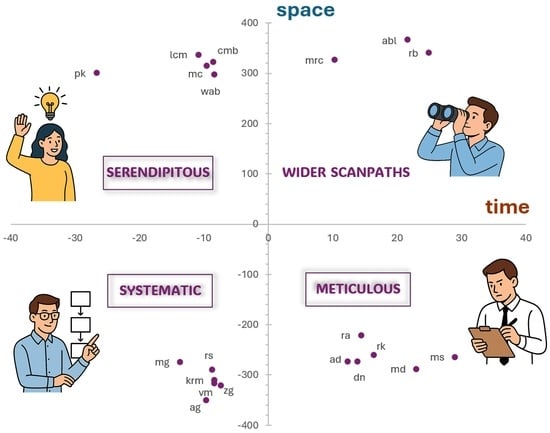
5.1. Participants’ Reading Speed and Reading Style: HT- and HS- 1,2, and 3

Comparing participants’ reading speed with the overall average and participants’ scanpath area with the overall average width revealed distinct reading styles. Figure 27 depicts participants’ reading patterns on a two-dimensional plane defined by fixation time and scanpath area MSEs. The first group comprises fast readers with small average scanpath areas (ag, zg, rs, vm, krm). The second group consists of slow readers with wider scanpaths on average (rb, abl, mrc). A third group is characterized by fast readers with wide scanpaths (lcm, wab, pk). A fourth group includes slow readers with smaller scanpaths (md, ra, dn, rk). These observations suggest three main styles. The labels for each group were arbitrarily assigned and were derived by our interpretation of the findings. In particular, the first group of readers showing a fast reading style with small eye movements may identify the intention to scan the whole information in a correct and complete way, possibly efficient so as to be repeatable (small and fast) without losing any detail. We call this way systematic (group 1). The fourth group of readers showing a slow reading style, and a smaller scanpath may reveal the intention to scan whole–complete–pieces of information at once, spending the necessary time to acquire it. We call this way meticulous (group 4). The third group of readers, characterized by a fast reading with a wider scanpath, may represent the intention to look at the data visualization in a scattered way, without a systematic or meticulous style, more like “wandering around” it. We call this way serendipitous (group 3). Finally, Group 2 may reflect effects of information disposition or fatigue, though it could also represent a meticulous variant. Thus, we do not propose a specific label for them. Figure 28 reports examples of the three reading styles for three participants, one for each group.

Further inspection of the more fine-grained analysis of Section 4 refines these categories. For example, participant lcm is, on average, the fastest across both shorter-to-read visualizations (area, bars) and longer ones (trees, networks), while also exhibiting significantly wider scanpaths. This supports a serendipitous style, likely influenced by complex data viz. Participant pk shows a related but distinct pattern: fastest with shorter visualizations (bars, maps) yet slowest with longer ones (diagrams). Participant sk is the fastest for very short visualizations (lines), with wide scanpaths for circles and maps, again suggesting a serendipitous style influenced by visualization design. Conversely, participant rb demonstrates an opposite speed pattern but similar scanpath width to lcm, suggesting a meticulous style. Participant pj is the slowest reader for 6 out of 11 visualization types, consistently with the highest MSE, despite these being generally faster types (area, bars, circles; see Figure 11), indicating unpredictable behaviour.

The swarm plot in Figure 11 enables comparison of average reading speed at the level of individual data, viz, capturing nuances and transitions among the three styles. Among the fastest readers, mg, ms, and ls show the highest speeds (leftmost blue and less sparse pink points). About one third of participants cluster in a mid-range, with MSE distributions concentrated in $(-20k,+20k)$, making them neither the fastest nor slowest. This “average performers” group includes readers spanning systematic to serendipitous styles: lcm, pi, wab, mc, em, cy, krm, mrc, vm, jm, ad. Another cluster shows longer and more dispersed reading speeds, with more uniform presence toward high MSE values, suggesting average performers leaning from serendipitous to meticulous styles (abl, cmb, db, rb, rk, sok).

The analysis of scanpath areas reveals further differentiation. One fifth of participants showed wider scanpaths for lines (221), diagrams (182), and tables (342), all characterized by scattered information. Five of these (abl, sok, rk, cmb, db) had previously been classified as serendipitous-to-meticulous in terms of speed. Conversely, nearly one third exhibited small scanpaths for bars, one fifth for lines, and one sixth for area and points. One fourth of participants had more predictable scanpaths, represented by uniform densities of blue or pink points (cmb, lcm, mc, mg, pi, rk, rb, wab). All processed the full set of 393 visualizations, except mc (295). Among those who processed 295–100 visualizations, one third displayed predictable scanpaths for faster types and less predictable ones for slower types (abl, ad, ch, em, krm, ls, md, pj, pk, ra, tj). Twelve participants who processed only 100 visualizations showed unpredictable scanpaths for both faster and slower types (ag, am, cy, dn, jm, mrc, ms, rs, sh, sk, vm, zg). These findings suggest that processing more visualizations increases scanpath predictability, while fewer visualizations correspond to more scattered patterns. This may reflect both prior ability and transient expertise developed during the task, shaped by visualization complexity and information disposition. More predictable behaviours (blue clusters) contrast with dispersed ones (pink clusters), the latter possibly reflecting fatigue bias [38].

Reading speed also varies systematically with visualization type. Area, bars, circles, and lines exhibit similar patterns, with low MSEs for most participants until a sharp rise for a few. Diagrams, distributions, and gridmatrix show bimodal patterns, with half of the participants reading very fast and half very slow, likely influenced by design. Maps and points tend to be slower, showing progressively steeper curves. The longest reading times are associated with tables, trees, and networks.

For area, points, and tables, participants were split evenly between significantly faster and significantly slower than average. Unlike reading speed, where leftmost MSE values rarely exceeded rightmost ones, scanpath areas sometimes do. For circles, scanpaths divide evenly between smaller and wider. For bars, maps, and trees and networks, smaller scanpaths dominate, while diagrams and gridmatrix show wider ones. Distributions show mostly smaller scanpaths, but with a very high rightmost MSE, denoting complexity.

Finally, analysis of average scanpath areas confirms the participant groupings described above. Participants lg, sok, and abl exhibit wider scanpaths for both longer-to-read types (diagrams, trees, networks) and shorter ones (bars). Two of them also belong to the meticulous group. Conversely, vm, ag, and zg show consistently smaller scanpaths, regardless of visualization type, aligning with the systematic group of faster readers.

5.2. Data Viz Complexity and Information Disposition: HT- and HS- 4 and 5

Figure 29 and Figure 30 show a summary scatterplot of correlations between time and space in characterizing data, viz, complexity using MSEs. The data suggest three clusters of visualization types: those with gathered information disposition, those with scattered disposition, and those characterized by higher intrinsic density and thus greater complexity.

This finding partly confirms earlier analyses: points, area, circles, and lines are, in this order, the fastest to read, whereas trees and networks and diagrams appear among the most complex. Notably, among the longest-to-read types, 6 out of 49 diagrams and 6 out of 10 trees and networks fall in this category. Figure 12 highlights a large difference (about 60k) between negative-wise and positive-wise bias MSEs, suggesting that positive-wise MSEs correspond to particularly complex visualizations.

For bars, both negative- and positive-wise MSEs remain below 40k, indicating that these are generally easy to read. Among circles, two cases (118, 127) are outliers: their MSE values, both negative- and positive-wise, are well above all others, suggesting they are not representative of the type. By contrast, diagrams consistently show higher positive-wise than negative-wise MSEs. Although the most complex diagram may not represent the whole type, the trend confirms that diagrams are often harder to read. In gridmatrix, visualizations 187 and 193 are respectively the most complex and easiest, but even with only four significant cases, a positive-wise bias is evident, indicating higher average complexity. For lines, negative- and positive-wise MSEs are generally similar, suggesting that, except for a few extreme cases, lines are mostly quick to read, a trend resembling that of bars. For maps, negative- and positive-wise MSEs are comparable, except for the longest-to-read case, implying they are usually easy, but design choices may reduce intuitiveness. The same applies to points, which behave similarly to area. Tables also follow this pattern. For trees and networks, despite only four significant cases, a clear positive-wise bias suggests they are generally more complex. In some cases, very complex visualizations (e.g., lines, maps, and especially diagrams) may require domain-specific knowledge, indicating that complexity is partly dependent on participants’ domain literacy.

5.3. Participants and Data Viz Through AOIs: HTS-6, 7, 8, and 9

Regarding AOIs, results are consistent with expectations: encoding required the longest reading time. As noted in earlier participant-level analyses, title was shorter to read but wider to scan. More surprisingly, scale was both the shortest to read and the smallest to scan, suggesting it is the most overlooked element. Similarly, footer was short to read and small to scan, though less unexpectedly. These findings indicate an overall pattern in which readers primarily access meaning through encoding and title as the main gateways to a visualization, while more detailed textual and numerical elements (scale, footer, label) receive secondary and superficial attention.

AOI reading patterns vary by visualization type. Bars, lines, and maps share similar profiles, with a balance of very short and very long cases. For points, nearly half of the visualizations are long to read, with higher MSE values. Area and circles include more short than long cases relative to other types. For bars and circles, encoding was shorter to read than in other types, and lines followed this pattern, whereas distributions and gridmatrix showed the opposite. In maps, encoding was longer, reflecting their intrinsic complexity. For points, patterns were more variable, suggesting dependence on data representation rather than type itself. Regarding scanpath area, in 8 of 11 types the widest AOI was title (Figure 26), confirming the back-and-forth reading behaviour identified earlier. Wider scanpaths were also observed for label and scale in shorter-to-read types (area, bars, circles, lines) as well as in maps and points, reinforcing their marginal role relative to encoding. Conversely, for distributions, gridmatrix, and tables, encoding was the widest AOI.

Detailed results in Figure 26 show that footer and scale consistently yielded smaller scanpaths, while title always exhibited wider ones. Encoding and label varied, with both small and wide areas. Specifically, encoding was smallest in lines, whereas in all other significant types it was wider; scale was smallest in maps.

Figure 25 further indicates that encoding, footer, and scale had balanced distributions, with half of the significant cases showing smaller scanpaths and half wider ones. By contrast, label almost always exhibited smaller scanpaths, confirming it as the most overlooked AOI across participants and types. Footer and scale appeared to depend more on individual reading styles. At the participant level, pj showed the longest reading time across AOIs except title. Participant abl spent more time on footer and scale, with wider scanpaths, supporting a meticulous variant style. Participant wab read encoding, label, and title quickly, as did pi (except for encoding). Participants cmb and lcm also read encoding, label, and scale quickly. Two complementary meticulous styles are evident: participant ra, slower on encoding and scale, and participant rb, slower on label and title, reflecting visual- vs. textual-focused meticulousness. Participants sok and ls had the widest scanpaths on encoding and title, and on encoding and scale, respectively, suggesting focused but differentiated reading strategies.

5.4. Limitations of the Study

The exploitation of data from an existing source, i.e., not collected directly, was justified in the Introduction. A derived choice that may have caused further noise in the analysis of data was the uncritical adoption of the Western culture and language, the classification, labelling, and metadata provided in the primary study. However, the primary study is in the literature (see, for example [20] and the many other papers listed in the MASSVIS page), and all these choices have been declared and motivated in the introduction and method sections. On the other hand, the main demographics were missing from the available data, and we could not carry out statistics by strata. Another limitation may be related to the selection of a subset of the data viz available, in order to compare them at the level of Areas of Interest (AOIs). However, inclusion and exclusion criteria have been given for selecting a representative subset of the available data, viz, and this selection procedure took several rounds of testing and calibration between the two authors, and was further discussed until a satisfactory agreement was reached. The use of the scanpath area instead of directly using the fixation coordinates may be seen as another possible limitation. However, this could be seen as an enrichment, rather than a limitation of the study, as we have applied the same logic as that of the well-known and mathematically sound concept of squared error, to yield a quadratic representation of the space that could better discriminate and amplify differences. Another possible limitation may be the application of our method to a dataset that includes static data viz only. Although we deem it important to test approaches to more interactive artifacts, there are more limitations to the availability of such artifacts with respect to static data viz, and also problems related to the comparability of disparate degrees of interactivity that may affect the fair balance of the experiments. A final limitation may be the lack of previous and contextual knowledge or exogenous variables to drive the analysis and explanations of the eye-tracking data results. With the yielded findings, we have demonstrated that stepping back from superstructures allows unseen and situated reading patterns, such as, for example, the drift to systematic behaviour described in the Section 5, which may be considered as independent from the previous expertise of participants, but rather due to the interaction with many data viz. On the contrary, this reading pattern could have been hidden by a priori constructs and ante-hoc explanations.

6. Conclusions and Future Work

This study aimed at analysing existing eye-tracking data in the Data Visualization domain through the lenses of a statistical model, the bias-noise model, which was never applied before to data of the kind considered here. Research questions were posed about what mere eye-tracking data analysis without any extra variable could say about the reading patterns of users during interaction with data viz. The data were analyzed from three perspectives: that of users, that of data viz, and that of AOIs inside data viz. A total of 22% of the tests on the fixation time variable and 44% of the tests on the scanpath area variable were statistically significant. These results allowed for the identification of reading patterns and reading speed of participants, also in relation to the reading complexity of data viz and data viz types, and the information disposition patterns in data viz. Also, the predictability of the reading speed, reading pattern, complexity, and information disposition was identified, analyzed, and discussed.

The main findings of our study are: (i) the identification of three reading patterns for participants, namely a meticulous style, a systematic style, and a serendipitous style; (ii) the identification of two information disposition styles for data viz types, namely gathered and scattered, and of a third property, namely density, characterizing very complex data viz; (iii) the identification of an evolving performance where the more data viz participants read, the more their reading becomes faster, systematic, and more predictable; (iv) encoding and title are considered the primary elements of attention, characterized by a back-and-forth reading pattern among the two, followed by the other AOIs; and, in less complex to read data visualization types such as bars, circles, and lines, the encoding part becomes, on average, shorter to read.

As a final consideration, beside the noticeable result of capturing that “one size does not fit all” either for single participants or for single data viz or data viz types, leaving a priori knowledge and experience of participants in the background allowed us to observe a situated improvement in the reading speed, pattern and predictability, the more data viz were processed by single participants. This seems to suggest that mere eye-tracking data can provide very useful information about users’ performance with data viz, and also provide suggestions about how to make data viz design more suitable [39]. Beyond the considerations coming from this analysis, we may claim that approaches such as eye-tracking during human-data interaction with data viz may enrich the profiling and customization of these kinds of interactions [40]. As Data Visualization deals with ever more crucial communication and decision-making tools for common people, citizens, and domain experts during time-critical settings [31], grasping the real-time evolving characteristics of users is of vital importance for enabling effective interventions of data-driven knowledge in the real world.

Some implications for future design practices may come from this study: the need to consider the peculiarity of participants in tandem with their reading habits, thus the need to extend the investigation to other than Western world cultures. Other factors influencing the performance should be tested: the contingent factors, such as the available time, the level of attention, and the degree of fatigue, besides their basic knowledge and level of expertise.

References

1. Majaranta, P.; Bulling, A. Eye tracking and eye-based human–computer interaction. In Advances in Physiological Computing; Springer: London, UK, 2014; pp. 39–65. [Google Scholar]
2. Hansen, D.W.; Ji, Q. In the Eye of the Beholder: A Survey of Models for Eyes and Gaze. IEEE Trans. Pattern Anal. Mach. Intell. 2010, 32, 478–500. [Google Scholar] [CrossRef]
3. Jarodzka, H.; Balslev, T.; Holmqvist, K.; Nyström, M.; Scheiter, K.; Gerjets, P.; Eika, B. Conveying clinical reasoning based on visual observation via eye-movement modelling examples. Instr. Sci. 2012, 40, 813–827. [Google Scholar] [CrossRef]
4. Liu, X.; Cui, Y. Eye tracking technology for examining cognitive processes in education: A systematic review. Comput. Educ. 2025, 229, 105263. [Google Scholar] [CrossRef]
5. Locoro, A.; Cabitza, F.; Actis-Grosso, R.; Batini, C. Static and interactive infographics in daily tasks: A value-in-use and quality of interaction user study. Comput. Hum. Behav. 2017, 71, 240–257. [Google Scholar] [CrossRef]
6. Koyuncu, I.; Firat, T. Investigating reading literacy in PISA 2018 assessment. Int. Electron. J. Elem. Educ. 2020, 13, 263–275. [Google Scholar] [CrossRef]
7. Brysbaert, M. How many words do we read per minute? A review and meta-analysis of reading rate. J. Mem. Lang. 2019, 109, 104047. [Google Scholar] [CrossRef]
8. Al-Moteri, M.O.; Symmons, M.; Plummer, V.; Cooper, S. Eye tracking to investigate cue processing in medical decision-making: A scoping review. Comput. Hum. Behav. 2017, 66, 52–66. [Google Scholar] [CrossRef]
9. Currie, J.; Bond, R.R.; McCullagh, P.; Black, P.; Finlay, D.D.; Peace, A. Eye Tracking the Visual Attention of Nurses Interpreting Simulated Vital Signs Scenarios: Mining Metrics to Discriminate Between Performance Level. IEEE Trans. Hum.-Mach. Syst. 2018, 48, 113–124. [Google Scholar] [CrossRef]
10. Lu, Y.; Sarter, N. Eye Tracking: A Process-Oriented Method for Inferring Trust in Automation as a Function of Priming and System Reliability. IEEE Trans. Hum.-Mach. Syst. 2019, 49, 560–568. [Google Scholar] [CrossRef]
11. Guo, Y.; Freer, D.; Deligianni, F.; Yang, G.Z. Eye-Tracking for Performance Evaluation and Workload Estimation in Space Telerobotic Training. IEEE Trans. Hum.-Mach. Syst. 2022, 52, 1–11. [Google Scholar] [CrossRef]
12. Grundgeiger, T.; Wurmb, T.; Happel, O. Statistical Modeling of Visual Attention of Junior and Senior Anesthesiologists During the Induction of General Anesthesia in Real and Simulated Cases. IEEE Trans. Hum.-Mach. Syst. 2020, 50, 317–326. [Google Scholar] [CrossRef]
13. Nielsen, J. F-Shaped Pattern for Reading Web Content, Jakob Nielsen’s Alertbox. 2006. Available online: http://www.useit.com/alertbox/reading_pattern.html (accessed on 24 August 2025).
14. Nielsen, J.; Pernice, K. Eyetracking Web Usability; New Riders: Thousand Oaks, CA, USA, 2010. [Google Scholar]
15. Gilhooly, K.J.; Sleeman, D.H. To differ is human: A reflective commentary on “Noise. A Flaw in Human Judgment”, by D. Kahneman, O. Sibony & CR Sunstein (2021). London: William Collins. Appl. Cogn. Psychol. 2022, 36, 724–730. [Google Scholar] [CrossRef]
16. Burch, M.; Kurzhalis, K.; Weiskapf, D. Eye Tracking Studies in Visualization: Phases, Guidelines, and Checklist. In Proceedings of the 2025 Symposium on Eye Tracking Research and Applications, Tokyo, Japan, 26–29 May 2025; pp. 1–7. [Google Scholar]
17. Ke, F.; Liu, R.; Sokolikj, Z.; Dahlstrom-Hakki, I.; Israel, M. Using eye-tracking in education: Review of empirical research and technology. Educ. Technol. Res. Dev. 2024, 72, 1383–1418. [Google Scholar] [CrossRef]
18. Oppenlaender, J. Multilaboratory Experiments Are the Next Big Thing in HCI. Interactions 2025, 32, 6–7. [Google Scholar] [CrossRef]
19. Wilkinson, M.D.; Dumontier, M.; Aalbersberg, I.J.; Appleton, G.; Axton, M.; Baak, A.; Blomberg, N.; Boiten, J.-W.; da Silva Santos, L.B.; Bourne, P.E.; et al. The FAIR Guiding Principles for scientific data management and stewardship. Sci. Data 2016, 3, 160018. [Google Scholar] [CrossRef] [PubMed]
20. Borkin, M.A.; Vo, A.A.; Bylinskii, Z.; Isola, P.; Sunkavalli, S.; Oliva, A.; Pfister, H. What makes a visualization memorable? IEEE Trans. Vis. Comput. Graph. 2013, 19, 2306–2315. [Google Scholar] [CrossRef]
21. Biber, D.; Reppen, R.; Friginal, E. Using corpus-based methods to investigate grammatical variation. In The Oxford Handbook of Linguistic Analysis; Heine, B., Narrog, H., Eds.; Oxford University Press: Oxford, UK, 2012; pp. 276–296. [Google Scholar]
22. Carter, B.T.; Luke, S.G. Best practices in eye tracking research. Int. J. Psychophysiol. 2020, 155, 49–62. [Google Scholar] [CrossRef] [PubMed]
23. Ruf, V.; Horrer, A.; Berndt, M.; Hofer, S.I.; Fischer, F.; Fischer, M.R.; Zottmann, J.M.; Kuhn, J.; Küchemann, S. A Literature Review Comparing Experts’ and Non-Experts’ Visual Processing of Graphs during Problem-Solving and Learning. Educ. Sci. 2023, 13, 216. [Google Scholar] [CrossRef]
24. Toker, D.; Conati, C.; Steichen, B.; Carenini, G. Individual user characteristics and information visualization: Connecting the dots through eye tracking. In Proceedings of the SIGCHI Conference on Human Factors in Computing Systems, Paris, France, 27 April–2 May 2013; pp. 295–304. [Google Scholar]
25. Borkin, M.A.; Bylinskii, Z.; Kim, N.W.; Bainbridge, C.M.; Yeh, C.S.; Borkin, D.; Pfister, H.; Oliva, A. Beyond memorability: Visualization recognition and recall. IEEE Trans. Vis. Comput. Graph. 2015, 22, 519–528. [Google Scholar] [CrossRef] [PubMed]
26. Bylinskii, Z.; Borkin, M.A.; Kim, N.W.; Pfister, H.; Oliva, A. Eye fixation metrics for large scale evaluation and comparison of information visualizations. In Eye Tracking and Visualization, Proceedings of the Foundations, Techniques, and Applications, ETVIS 2015, Chicago, IL, USA, 25 October 2015; Springer: Cham, Switzerland, 2017; pp. 235–255. [Google Scholar]
27. Kim, N.W.; Bylinskii, Z.; Borkin, M.A.; Gajos, K.Z.; Oliva, A.; Durand, F.; Pfister, H. Bubbleview: An interface for crowdsourcing image importance maps and tracking visual attention. ACM Trans. Comput.-Hum. Interact. (TOCHI) 2017, 24, 1–40. [Google Scholar] [CrossRef]
28. Kosara, R. Evidence for area as the primary visual cue in pie charts. In Proceedings of the 2019 IEEE Visualization Conference (VIS), Vancouver, BC, Canada, 20–25 October 2019; pp. 101–105. [Google Scholar]
29. Keller, C.; Junghans, A. Does guiding toward task-relevant information help improve graph processing and graph comprehension of individuals with low or high numeracy? An eye-tracker experiment. Med. Decis. Mak. 2017, 37, 942–954. [Google Scholar] [CrossRef]
30. Kahneman, D.; Sibony, O.; Sunstein, C. Noise: A Flaw in Human Judgment; William Collins: Glasgow, UK, 2021. [Google Scholar]
31. Cabitza, F.; Locoro, A.; Batini, C. Making open data more personal through a social value perspective: A methodological approach. Inf. Syst. Front. 2020, 22, 131–148. [Google Scholar] [CrossRef]
32. Itti, L.; Koch, C.; Niebur, E. A model of saliency-based visual attention for rapid scene analysis. IEEE Trans. Pattern Anal. Mach. Intell. 2002, 20, 1254–1259. [Google Scholar] [CrossRef]
33. Franzen, L.; Stark, Z.; Johnson, A.P. Individuals with dyslexia use a different visual sampling strategy to read text. Sci. Rep. 2021, 11, 6449. [Google Scholar] [CrossRef] [PubMed]
34. Ware, C. Information Visualization: Perception for Design; Morgan Kaufmann: Burlington, MA, USA, 2019. [Google Scholar]
35. Liang, K.; Chahir, Y.; Molina, M.; Tijus, C.; Jouen, F. Appearance-based eye control system by manifold learning. In Proceedings of the 2014 International Conference on Computer Vision Theory and Applications (VISAPP), Lisbon, Portugal, 5–8 January 2014; Volume 3, pp. 148–155. [Google Scholar]
36. Wang, D.; Formica, M.K.; Liu, S. Nonparametric Interval Estimators for the Coefficient of Variation. Int. J. Biostat. 2018, 14, 1–15. [Google Scholar] [CrossRef]
37. Nakagawa, S. A farewell to Bonferroni: The problems of low statistical power and publication bias. Behav. Ecol. 2004, 15, 1044–1045. [Google Scholar] [CrossRef]
38. Hecht, R.M.; Hillel, A.B.; Telpaz, A.; Tsimhoni, O.; Tishby, N. Information Constrained Control Analysis of Eye Gaze Distribution Under Workload. IEEE Trans. Hum.-Mach. Syst. 2019, 49, 474–484. [Google Scholar] [CrossRef]
39. Blundell, J.; Collins, C.; Sears, R.; Plioutsias, T.; Huddlestone, J.; Harris, D.; Harrison, J.; Kershaw, A.; Harrison, P.; Lamb, P. Multivariate Analysis of Gaze Behavior and Task Performance Within Interface Design Evaluation. IEEE Trans. Hum.-Mach. Syst. 2023, 53, 875–884. [Google Scholar] [CrossRef]
40. Li, F.; Chen, C.H.; Xu, G.; Khoo, L.P. Hierarchical Eye-Tracking Data Analytics for Human Fatigue Detection at a Traffic Control Center. IEEE Trans. Hum.-Mach. Syst. 2020, 50, 465–474. [Google Scholar] [CrossRef]
Figure 1. An example of ten data visualizations included in the MASSVIS Project. Colored labels show their classification type, as reported in [20].
Futureinternet 17 00504 g001
Figure 2. A line chart included in the subset of 63 MASSVIS pictures for which an AOI layer is depicted. For copyright reasons, only the visual part is reported (title, legend, and footer were deleted). Red boxes were drawn and superimposed on each of the 63 data viz selected in order to manually inspect AOIs and observe all the fixation points inside that box (an orange to purple bubble represents the number of fixation points in that point of the picture). A heatmap allows the scrutiny of scanpath patterns (where bubbles are larger and lighter, there were more fixations, where bubbles are smaller and darker, there were fewer fixations).
Futureinternet 17 00504 g002
Figure 3. The geometrical relationship between MSE and its components. The idea of representing MSE as A Pythagorean chart was borrowed by [30]. In particular, the relationship between MSE and bias and noise (being MSE the sum of the squares of both bias and noise) is rendered visually. The MSE area of the square is equal to the area of the bias + area of the noise squares, and bias and noise are related by a proportional relation in the MSE measure. Assuming 1, the area of MSE, bias, and noise can have different proportion combinations, all summing to 1 (e.g., 0.4–0.6; 0.5–0.5, etc.).
Futureinternet 17 00504 g003
Figure 4. Building vector spaces from fixation locations. On the left, a linear scanpath can be observed; on the right, a quadratic scanpath (the coverage area) can be observed. We assume that the dot product vector operation is direction-invariant (as it only involves the magnitude and angle of vectors).
Futureinternet 17 00504 g004
Figure 5. Flow diagram of our experimental setup.
Futureinternet 17 00504 g005
Figure 6. Testing for the non-normality of the time of fixation and fixation vector dot products.
Futureinternet 17 00504 g006
Figure 7. Descriptive statistics for fixation time and scanpath area aggregated by data viz type. (a) Violin plots of the fixation time variable (y axis), aggregated by data viz type (x axis). Outliers are cut at the threshold of 500 ms. (b) Violin plots of the scanpath area variable (y axis), aggregated by data viz type (x axis).
Futureinternet 17 00504 g007
Figure 8. Descriptive statistics for fixation time and scanpath area at AOI level. (a) Violin plots of the fixation time variable, aggregated by AOI. Outliers are cut at the threshold of 500 ms. (b) Violin plots of the scanpath area variable, aggregated by AOI.
Futureinternet 17 00504 g008
Figure 9. Participants ID (y axis) and their reading speed MSE (x axis) vs. the average reading speed of all participants, ordered by MSE.
Futureinternet 17 00504 g009
Figure 10. Participant’s reading speed MSE vs. data viz type average reading speed of some data viz types.
Futureinternet 17 00504 g010
Figure 11. Participant’s reading speed MSE vs. single data viz average reading speed, ordered by MSE. The blue are those data viz shorter to read, the pink are those data viz longer to read, by each participant. Outliers were cut at an MSE of 120 k .
Futureinternet 17 00504 g011
Figure 12. Single data viz reading speed MSE vs. data viz type average reading speed, for some data viz types.
Futureinternet 17 00504 g012
Figure 13. Data viz type reading speed MSE vs. whole dataset average reading speed, ordered by MSE.
Futureinternet 17 00504 g013
Figure 14. AOIs reading speed MSE vs. whole dataset average reading speed, ordered by MSE.
Futureinternet 17 00504 g014
Figure 15. AOIs reading speed MSE of single data viz vs. data viz type average reading speed, for some data viz types.
Futureinternet 17 00504 g015
Figure 16. AOIs reading speed MSE of single participants vs. AOI reading speed.
Futureinternet 17 00504 g016
Figure 17. AOIs (first three letters) reading speed MSE for data viz type (last letter) vs. AOIs average reading speed, ordered by AOI and its MSE.
Futureinternet 17 00504 g017
Figure 18. Participants. ID (y axis) and their reading pattern MSE (x axis) vs. all participants’ average reading style, ordered by MSE.
Futureinternet 17 00504 g018
Figure 19. Participant’s scanpath area MSE vs. data viz type average scanpath area, for some data viz types.
Futureinternet 17 00504 g019
Figure 20. Participant’s scanpath area MSE vs. single data viz average scanpath area, ordered by MSE. Outliers were cut at an MSE of 2M (all the outliers cut were those at the right extreme).
Futureinternet 17 00504 g020
Figure 21. Data Viz scanpath area MSE vs. data viz type average scanpath area, for some data viz types.
Futureinternet 17 00504 g021
Figure 22. Data Viz type reading pattern MSE vs. whole dataset average reading style, ordered by MSE.
Futureinternet 17 00504 g022
Figure 23. AOIs reading style MSE vs. whole dataset average reading pattern, ordered by MSE.
Futureinternet 17 00504 g023
Figure 24. AOIs scanpath area MSE vs. single data viz by type average scanpath area, for some data viz types.
Futureinternet 17 00504 g024
Figure 25. AOIs scanpath area MSE vs. data viz type average scanpath area.
Futureinternet 17 00504 g025
Figure 26. AOIs reading pattern MSE for data viz type vs. AOIs average reading style, ordered by AOI and MSE.
Futureinternet 17 00504 g026
Figure 27. Map of the resulting Data Visualization Reading Pattern emerging from eye-tracking data analysis. Axes values (all in thousands) are MSE values; the x-axis represents fixation time MSE, the y-axis scanpath area MSE. All results are only those statistically significant at the participant level. The top right quadrant shows an unlabelled reading pattern, we left the question mark to indicate it.
Futureinternet 17 00504 g027
Figure 28. The three reading styles as interpreted for the three groups of participants: serendipitous (no regular trajectory–the arrows, nor specific order in visiting elements in the scanpath–the red bubbles–for participant wab), systematic (shorter and ordered–left to right arrows–fixations for ag), and meticulous (a selective scanpath trajectory focused on the salient elements of the data viz such as title, visual encoding and labels (see both arrows and red bubbles), for dn) on the same data viz (blank patches cover different parts the three background figures, which were also blurred, for copyright reasons).
Futureinternet 17 00504 g028
Figure 29. Map of the resulting Data Visualization Reading Complexity emerging from eye-tracking data analysis. Axes values (all in thousands) are MSE values; the x-axis represents fixation time MSE, the y-axis scanpath area MSE. All results are only those statistically significant at the data viz type level.
Futureinternet 17 00504 g029
Figure 30. Examples of three data viz types with a layer of fixation bubbles (each bubble size is proportional to the number of fixations, and the bubble colour shows the same proportion, from the darker, smaller, to the lighter, bigger, bubbles).
Futureinternet 17 00504 g030