1. Introduction
The Internet of Things (IoT) has become a cornerstone of modern networks. the IoT, a term synonymous with the interconnectivity of “Things”, has led to internet-facing devices flooding the markets in recent years, with a prediction of approximately 25 billion devices by 2030 [
1]. This rapid expansion has led many companies to release their IoT product into the growing market as fast as possible. Security is often a second thought, or not considered at all for many of these devices, as it would only slow down production. As such, the market overflows with an ocean of insecure, unprotected and, in some cases, hazardous IoT devices [
2]. Indeed, the expansive Internet of Things has vastly spread the attack surface for the average citizen, likely exposing them in ways they do not even consider.
For example, in 2021, the cloud-based security camera service Verkada was breached after malicious actors discovered viable admin credentials on the internet, exposing the live feeds of over 150,000 cameras worldwide [
3]. These cameras were located in hospitals, classrooms, jails, factories and many other sensitive locations. Poor user privilege hygiene emerged as the leading cause of the breach, with over 100 Verkada personnel having ‘super admin’ permissions. Even without the breach, this was a significant infringement of customers’ privacy as these super admins had access to clients’ live feeds, likely without the customers’ knowledge.
In the same year, critical national infrastructure was attacked in Florida, USA. This time, the target was a city’s water treatment facility [
3]. Malicious actors accessed a plant employee’s computer remotely and, using the applications on this PC, adjusted the water’s sodium hydroxide (NaOH) levels by a factor of 100. This might have proven to be one of history’s most deadly cyber attacks, if not for swift intervention from the facility, readjusting the chemical levels. This attack illustrates the potential danger of outdated systems, which most critical national infrastructures rely upon, and the danger of omitting safety systems from critical infrastructure. If a safety system (for example, requiring two operators to authorise the change in chemical concentrations far outside normal specifications or the swiping of a physical key card to authorise the operation) was used, it would have made it much harder for attackers.
Due to the unique, and often resource-constrained nature of the IoT ecosystem, traditional security practices cannot be easily applied. Extensive research has been conducted in signature-based intrusion detection systems (IDSs) and anomaly detection-based IDSs for IoT devices to detect cyber attacks. Typically, signature-based IDS relies on training with well-known normal and attack signatures, exhibiting high performance on previously encountered attacks but limited capability to handle unpredictable or unseen zero-day attacks. On the other hand, anomaly-based detectors operate by identifying deviations from the baseline, usually trained solely on normal behaviour. They excel at detecting unseen attacks but may not perform as well as signature-based approaches with well-known attacks.
Parallel to the growth of IoT in recent years, artificial intelligence (AI) has seen substantial growth in activity and use, especially in security. Fully supervised AI approaches have been deployed for signature-based detection in IDSs and, more recently, semi-supervised and unsupervised approaches have been deployed for anomaly detection in IoT. These recent approaches will be reviewed in the related works
Section 2.
One main limiting factor disadvantaging security operators is the lack of training data. This training data can be considered both from the perspective of training humans on attack patterns to understand and mitigate them and training automated AI-based detection methods. In our previous work [
4], we discussed IoT security from a somewhat unconventional point of view, focusing on device power consumption (as a linear time series) rather than internet packets. In that work, we attempted to illustrate that studying these signatures from a human perspective is an invaluable asset for security teams in understanding how the attacks work and how to defend against them. Importantly, we showed that device power, while not as readily available as internet traffic, should not be overlooked in security. To this end, we adopt some key concepts from popular side-channel attack methodologies, e.g., simple power analysis (SPA) and differential power analysis (DPA) [
5], to study the power signatures for use in security. The more data sources and defensible positions we consider in security research, the more we can close the gap between attacker and defender.
To this end, we present Dragon_Pi, which is an IoT power dataset containing labelled normal and attack scenarios captured from two of the most popular IoT platforms (Raspberry Pi and Snapdragon). We also present Dragon_Slice, which is the first attempt at designing an automated IDS based on these data. Dragon_Pi fills a fraction of the massive gap in IoT security. To the best of the authors’ knowledge, Dragon_Pi and Dragon_Slice, respectively, constitute the first publicly available IoT security power dataset and unsupervised convolutional autoencoder based on IoT power consumption. Dragon_Pi is the first step of many in supplementing traditional security approaches to IoT security using side-channel data, such as power consumption. We invite others to repeat the process and generate datasets of a similar nature, exploring IoT security from a different perspective.
1.1. Contributions
The Dragon_Pi, Dragon_Slice framework extends our previous work [
6]. Indeed, this work can be considered as part two of our recent work [
4], where we discuss and analyse the signatures of both normal and attack behaviours within the Dragon_Pi dataset. This recent work seeks to illustrate the value of power data in cybersecurity and discuss possible usages. Dragon_Pi and Dragon_Slice seek to fulfil some of the possible works that we said were possible based on the data in [
4,
6]. The specific contributions are as follows:
- 1.
Dragon_Pi: The first contribution is a fully labelled device power behaviour dataset containing normal and attack scenarios from two popular IoT devices. Dragon_Pi explores various attack scenarios and, to the authors’ knowledge, is the only publically available IoT Security power dataset. Dragon_Pi focuses on IoT devices, and the insights gained from studying this dataset can be applied to the entire cybersecurity field. Dragon_Pi serves as a step forward for IoT security, encouraging security professionals to consider as many data sources as possible rather than focus on internet traffic.
- 2.
Dragon_Slice: The second contribution is Dragon_Slice for anomaly detection within linear time series. Importantly, Dragon_Slice is a single model trained only on the normal power behaviours of both the DragonBoard and Raspberry Pi. Using the Dragon_Slice framework, a single IDS model can be trained on the normal power consumption data of different devices. This model can then detect unseen anomalies across the different devices. This is a massive contribution to the field of IoT, which is filled with heterogeneous devices. In this way, a single model can serve as many devices as desired, rather than requiring specifically trained models per device type.
- 3.
Explainability: The third contribution involves explaining the AI used in this paper. To this end, we explain Dragon_Slice from the perspective of inputs and outputs, and, thus, why the AI is making particular decisions. In AI research, many works under-explain the presented AI. This hinders readers from effectively understanding what the AI is doing or from reconstructing similar AI for themselves. Another key issue with under-explained AI is the lack of verification of the AI functionality. Readers can only confirm the plausibility of the presented results if they are able to understand the AI demonstrated.
1.2. Organisation
The remainder of this work is organised as follows.
Section 2 surveys some of the most popular IoT security datasets and some recent AI applied to those datasets.
Section 3 discusses the over-arching framework and a brief overview of the dataset itself.
Section 4 describes the Dragon_Slice architecture and training methodology as well as the results from the two paths taken for the AI.
Section 5 discusses some of the key findings of the study and further explains some aspects of the architecture. Limitations of the study are discussed in
Section 6. The conclusions and possible further works are presented in
Section 7.
2. Related Works
As IoT Security is an emerging and essential field, much work has been conducted to create automated security systems (such as IDSs) for them. Much of this research has used AI to secure these IoT systems. AI is a pervasive paradigm within most recent technology fields and has seen great success in IoT security and the wider security field.
Before any AI algorithm can be trained, there must be data available to train and test upon. As such, a large and vital portion of IoT security research has involved creating and labelling datasets of IoT attack data. The data must be realistic, relevant, and of good quality.
Much surveying has been conducted in the field of IoT intrusion detection [
7,
8,
9], in particular, presented extensive research on a wide range of algorithms used by researchers and summarised the popularity of well-known datasets in the reviewed work. Importantly, they realised that most of the works they surveyed used simulated or outdated datasets. This clarifies the need for as many new and up-to-date datasets as possible in cybersecurity and IoT security. The overuse of outdated datasets has led to research results, which may not translate to acceptable performance in the modern cyber threat topography.
Table 1 lists some well-known datasets chronologically, along with their proportionate usage in [
9].
In [
9], the oldest work they reference is from 2016; when consulting
Table 1, we can see a disproportionate percentage of papers using outdated datasets. The fact that researchers must rely on such outdated data illustrates the distinct lack of data in the field of IoT cybersecurity and, thus, motivates the creation of the Dragon_Pi dataset presented in this work. By consulting
Table 1, it is also clear that the overwhelming majority of the dataset work conducted on IoT focuses entirely on network packets. While this makes sense, since cybersecurity has been dominated by network-based security for decades, it is imperative to consider security from as many points of view as possible in the modern cyber threat topography.
Derived from the 1998 Defence Advanced Research Project Agency (DARPA) dataset [
35], the Knowledge Discovery and Data Mining (KDD) 1999 dataset was created to be used in the development of security-focused ML [
10,
11]. In essence, the KDD dataset transforms the DARPA dataset’s network traces into a collection of features found in the connection between two hosts, with each connection constituting its own record in the dataset. These features are broken into basic (e.g., duration), content (e.g., logged_in), time-based (e.g., srv_count), and connection-based (e.g., dst_host_count) categories.
Due to its acceptance as a de facto benchmark for cybersecurity research, many research works today are still conducted using the KDD dataset, regardless of its age and, indeed, its outdatedness. In 2019, ref. [
13] applied three different artificial neural network (ANN) approaches to the KDD dataset. Utilising learning vector quantization (LVQ), the radial basis function (RBF), and multilayer perceptron (MLP), they achieved accuracies of 97.5%, 99.4%, and 99.86%, respectively. Notably, however, the presumably inference time performance of the algorithms was compared, and it was found that LVQs were far more time efficient, requiring only 4.56 s for the best-performing model, with time requirements of 22,610 s for RBFs and 28,811 s for MLPs.
In 2022, ref. [
12] compared K-nearest neighbour (K-NN), support vector machines (SVMs), and a novel hybrid approach utilising the SNORT IDS [
36] and a naïve Bayes (NB) algorithm on the KDD 99 dataset. In this hybrid approach, traffic is first analysed by the SNORT IDS and, if SNORT classifies the traffic as normal, the NB algorithm is applied to the traffic to confirm the result. The work achieved results of 93% for SVMs, 94.4% for K-NNs, and 96.6% for the proposed SNORT-NB hybrid model.
Given the infancy of networking security at the time, the KDD dataset naturally leaves much to be desired, being one of the first of its type in the field. In the decades since its release, the dataset has garnered much criticism; for example, in [
14], the authors present the argument that excess redundant and duplicate records are some critical shortfalls of the KDD dataset. In 2009, they created NSL-KDD, a shorter and more curated version of the KDD dataset. They achieved this by removing duplicate records or, more precisely, records that seemed like duplicates, which were generated during the creation process of the KDD dataset. Notably, in the creation process of the KDD dataset, the start time of connection, source, and destination IP addresses and source and destination ports were stripped from the internet packets. Thus, many traffic flows, such as ICMP, resulted in what appeared to be duplicated and redundant traffic flows, as they were missing these five key pieces of information that could distinguish them.
In 2016, ref. [
17] proposed a hybrid approach to IoT security. A proposed framework based on the MapReduce architecture was developed with the goal of distributed detection capabilities. Importantly, this framework considered IoT security from two key perspectives: internet traffic and wireless sensor network (WSN) traffic. The proposed framework featured both misuse-based and anomaly-based methodologies, utilising optimum path forest models. Based on the RPL routing protocol, a WSN was created to simulate the 6LoWPAN traffic. For the internet traffic aspect of the framework, the NSL-KDD dataset was implemented. The proposed hybrid approach achieved detection rates (DRs) of 80.95% and 96.20% for the anomaly detection and misuse-based modules, respectively. These modules also achieved false alarm rates (FARs) of 5.92% and 1.44%, respectively. Notably, the misuse-based model focused on internet traffic, while the anomaly detection model focused on the generated WSN traffic.
In 2017, ref. [
16] proposed an unsupervised conditional variational autoencoder (CVAE) IoT network-IDS (NIDS) trained on the NSL-KDD dataset. The architecture integrates intrusion labels within the decoder layers, and the approach boasts better performance than other unsupervised approaches, with a multi-class accuracy of 80.10%, all while being less complex. An essential aspect of the proposed architecture is the ability to reconstruct features from incomplete training sets, in particular, the protocol, flag, and service features, with accuracies of 99.02%, 92.84% and 71.42%, respectively. This is an important feature for the KDD and NSL-KDD datasets, which lost much information when the KDD dataset was created from the DARPA dataset. This framework introduced the first algorithm capable of performing feature recovery while also being the first work to present a CVAE in network intrusion detection.
To combat the lack of comprehensive network-based datasets, UNSW-NB15 [
19] was created. Previous benchmarks, DARPA98, KDD99, and NSL-KDD09, had become significantly outdated. Thus, UNSW-NB15 was generated to provide a dataset representing modern network traffic, information regarding the depth structure of the network, and minimal footprint intrusion. UNSW-NB15 contains real normal network traffic mixed with synthesised attack traffic.
In 2021, ref. [
22] proposed an edge-centric NIDS utilising deep neural networks, particularly long short-term memory (LSTM) models and gated recurrent units (GRUs), with the specific goal of DDoS detection in IoT. The model was trained and evaluated on the UNSW-NB15 dataset, achieving a high accuracy of 99%. The model proposed in the framework is lightweight and requires few resources, allowing for implementation in resource-constrained environments, such as the IoT. In [
22], the proposed framework models were deployed on Raspberry Pi, and their resource usage was compared to find the most suitable model for IoT, balancing accuracy with resource usage. From this comparison, it was found that the FastGRNN (fast-gated recurrent neural network) was the most suitable, with an accuracy of 99.95% and reasonably small resource requirements and inference times.
In 2022, ref. [
20] presented an IDS for IoT trained on the UNSW-NB15 dataset. The proposed framework utilised particle swarm optimisation-based gradient descent (PSO-LightGBM) for feature extraction. These features were then fed into a one-class SVM (OC-SVM) for classification between normal and anomalous. Evaluating the UNSW-NB15 dataset, the framework achieved an accuracy of 86.68%. The framework was specifically robust at detecting small sample data within UNSW-NB15, such as Shellcode, Worms, and Backdoor.
To mitigate the threat caused by compromised IoT devices, as well as develop a technique that can differentiate between hours-long and seconds-long attacks, the N-BaIoT [
23] model, and the resulting dataset, were created in 2018. N-BaIoT is an IoT NIDS framework that can extract snapshots from network traffic behaviour of interest and detect compromised IoT devices using deep autoencoders. To generate the data for training and testing, testbeds consisting of commercially available IoT devices were infected with the Mirai and BASHLITE IoT-based botnets. The proposed methodology had a true positive rate (TPR) of 100% detecting attacks launched from a compromised IoT device with a low false positive rate (FPR) of 0.007% and only between 174 ms and 212 ms to detect an attack.
In 2023, ref. [
27] proposed a semi-supervised AE approach to the N-BaIoT dataset. To cope with the scalability of IoT, the proposed framework allows for the training of a single model, which can work across many devices. The N-BaIoT dataset was split into multiple datasets based on the separate IoT devices in the testbed. The Deep AE was then trained on only the normal traffic flows from separate IoT devices, with the malicious traffic constituting separate test sets based on different IoT devices. The proposed approach achieved high performance with an all-in-one F1 score of 0.9996–0.9998, depending on the specific IoT device.
Thus far, recent decades have brought very few IoT-based intrusion detection benchmark datasets. The datasets released all have the common theme of capturing normal and malicious network traffic only, without any new data vectors included for cybersecurity research. To combat the lack of available benchmarks and provide a new avenue of data to explore for data-driven IDS, the ToN_IoT [
28] telemetry dataset was developed and released in 2020. ToN_IoT includes not only the network traffic of the IoT network but also the operating system logs and telemetry data of IoT services. ToN_IoT has an advantage over other datasets in the area as it contains IoT telemetry data and diverse attack scenarios, a representative and realistic testbed with IoT scenarios, labels for the data, and heterogeneity of IoT data sources. Many machine learning approaches were explored, such as logistic regression (LR), linear discriminant analysis (LDA), K-nearest neighbour (k-NN), classification and regression tree (CART), random forest (RF), naïve Bayes (NB), support vector machines (SVMs), and long short-term memory (LSTM). The machine learning algorithms first were evaluated on specific device datasets, i.e., fridge sensor (best performance: LSTM with 100% accuracy), garage door (best performance: all methodologies with 100% accuracy), GPS sensor (best performance: k-NN with 88% accuracy), Modbus (best performance: CART with 98% accuracy), Light_Motion (best performance: all approximately 58% accuracy), thermostat (best performance: all approximately 66% accuracy) and, finally, weather (best performance: CART with 100% accuracy). Combining all individual IoT device datasets into one, the CART approach emerged as dominant with an overall accuracy of 88% for binary classification and 77% for multi-class classification.
As part of the Avast AIC lab, the IoT-23 [
31] dataset was published in 2020. The dataset contains labelled traffic flows of benign and malicious behaviour captured between 2018 and 2019. IoT-23, named because it consists of 23 separate scenarios, contains over 300 million labelled records from sixteen categories, each record having eighteen features. These features are divided into static, basic, content, and time.
In 2021, ref. [
33] described designing and developing a convolutional neural network (CNN) for IoT network anomaly detection. Using the IoT-23 [
31] dataset, the multi-class CNN model was initially evaluated. CNNs using 1D, 2D, and 3D convolutions were then evaluated. Then, using transfer learning, a binary classifier CNN was trained from these initial multi-class models. In this use case, transfer learning from multi to binary classification proved effective as the binary classifier was trained on a subset of the data used to train the multi-class classifier. Over the datasets mentioned above, both the binary and multi-class classifiers achieved average accuracies of over 99% for 1D, 2D, and 3D CNN models.
In particular, in the field of cyber security, and as witnessed in the majority of datasets and the works reviewed above, security datasets tend to be focussed on one data vector: network traffic. This can easily be justified as the main avenue to explore in cybersecurity, as the network tends to be the key ingress point for most malicious activity. But even if network traffic is the main defence concern, exploring other data types within the security spectrum is also important. One main concern for most authors is the distinct lack of IoT-based internet traffic datasets—if datasets are sparse in the most explored area in IoT security, how much more sparsity is there in other data types? TON_IoT [
28] is one work that seeks to bring new data types to the cybersecurity dataset repertoire; however, the field remains completely unsaturated in all forms of data. As such, the work presented in this Dragon_Pi study calls for more datasets in the field. Only by exploring as many avenues for security as possible will defence personnel be empowered to catch up to the ever-adapting malicious actors.
Table 2 summarises the performance of the reviewed works on the reviewed datasets.
Regarding alternative data types, some research has been conducted into anomaly detection using various types of time series data.
In [
37], a reconstruction-based approach to anomaly detection in the linear time series was taken. Autoencoder-based models were utilised in the anomaly detection process, which is similar to the research presented in this work. Rather than fine-tune hyperparameters by hand, a neural architecture search technique was employed to find the best model configuration. A custom dataset that included time series features, such as temperature and luminance, CO
2 concentration, power consumption, and humidity, was used to train the AE models. Notably, the authors had no access to an anomaly detection dataset during testing; as such, synthetic anomalies were injected into the normal behaviour of the custom dataset during testing.
Generally, deep learning requires a vast amount of labelled data to train a model effectively. When working with real-world times series, the data collection is thought to be easy; the annotation of data, however, is time-consuming and relatively expensive. The works surveyed in [
38] demonstrate a solution to this problem through deep transfer learning. In essence, deep transfer learning allows for the training of a model on a far more extensive or diverse dataset, even if it is unrelated to the current problem. This pre-trained model gains far more general features from the larger datasets, which can be transferred effectively to the target problem during the fine-tuning stage on the much smaller and more limited dataset.
Another concern stemming from the lack of data in cybersecurity is the performance creep of many models on these well-known benchmark datasets. Part of the survey performed in this work is to illustrate that, even in recent years, studies are still being conducted on decades-old and obsolete datasets, likely due to the lack of available data. With datasets so over-explored, researchers may feel the need to set themselves, attempting techniques that may end up negating the validity of their model, such as the biased selection of samples for training and testing as a subset of an overall dataset. Far too many models are achieving results of 99% and 100% on datasets. These results are unlikely to transfer to real-life scenarios and should strongly indicate that either the model or dataset is lacking (either with models trained on the path of least resistance features, or datasets far too simple for the ever-adapting cyber landscape).
There is a clear need for more datasets as well as datasets of varying data types. This need guides the research that follows in this study. Dragon_Pi and Dragon_Slice represent initial steps to explore the effectiveness of power consumption data in security. The insights gained during this study will guide future efforts to incorporate heterogeneous data sources into the security pipeline.
3. Materials and Methods
3.1. Testbed, Data Acquisition, and Framework
For the testbed, two different IoT devices were chosen: Raspberry Pi 3 Model B and DragonBoard 410. DragonBoard, powered by a Qualcomm Snapdragon 410 processor, has gained widespread popularity, boasting over 200 million units shipped. Similarly, Raspberry Pi, a prevalent single-board computer, has seen a significant market presence with over 40 million units sold over its ten-year history.
Despite variations in manufacturers and typical applications, both devices surprisingly share almost identical specifications, possessing Quad Core 1.2 GHz 64-bit CPUs and 1.2 GB of RAM; this deliberate selection aims to provide a thorough understanding of common attack signatures across devices of different manufacturers, software, etc. Our previous study [
4] investigated whether these signatures exhibit general patterns, possibly simplifying the detection and understanding of attacks on IoT devices and heterogeneous networks. The previous work justifies the choice of devices and further explains other aspects of the device operation and testbed composition.
Both boards were connected to the internet via Wi-Fi, and SSH was enabled to broaden the potential attack surface. Bluetooth functionality enabled communication with a TI CC2650STK SensorTag, equipped with ten low-power MEMS sensors. A Python script on the testbed requested sensor data over Bluetooth, and DragonBoard and Raspberry Pi were linked to an Agilent Technologies N6705A DC Power Analyzer to unobtrusively monitor side-channel IoT power behaviour.
The framework, outlined in
Figure 1, proposes a generic data acquisition framework for IoT. This framework was initially proposed in our previous work [
4]. In addition to the previous framework,
Figure 1 showcases the focus of this current study, emphasising AI-based anomaly detection in IoT security based on the power acquisition framework. In this framework, power consumption data serve as input to the AI security system, returning a classification of either normal or anomalous for each power data segment.
The convolutional autoencoder (CAE) architecture employed in this study operates on the principle of reconstruction, where the AI attempts to reconstruct the input based on what it was trained on. In the case of the framework in this study, the AI is trained only on “clean-room” normal data obtained from the testbed. In this case, “clean room” describes a situation where the normal data were sampled and held aside, almost like it was quarantined in a different room. As such, the training set and test set are mutually distinct, and the training and test sets are two separate datasets, with one sampled in a quarantined environment with no anomalies and one with more real-world events and attacks.
During testing, real-world normal and attack data are passed to the AI, which attempts to reconstruct these inputs. If trained properly, a CAE should be able to reconstruct normal unseen data well, as they are similar to the training data. However, this methodology should struggle to reconstruct the anomalous attack data, which looks different from the normal baseline. The quality of the reconstruction and the resultant mean squared error (MSE) lead to a normal or anomaly classification (with low error meaning normal, and high error meaning anomaly).
This framework results in quite explainable AI, where the reconstructed output provides insights into what the AI perceives as normal or anomalous within the input signal, aiding in understanding the factors influencing its decision. This can significantly aid security experts in further identifying an attack or, possibly, a false positive from the AI output. Further analysing these factors would allow human intervention within the AI loop, or hierarchical AI, to oversee the output of many models. Human experts can assess both the input and output, making crucial decisions regarding security procedures. While the system can function autonomously, human oversight is vital as certain decisions can only be partially entrusted to AI. For example, AI can detect anomalous activity on a critical system, such as radar or health monitoring equipment. However, only a human can be responsible for making the call to shut down that device.
In hierarchical approaches, federated models could greatly enhance the system’s capabilities. Individual models could operate per device, or IoT gateway, overseen by a hierarchical AI that could supervise the models’ outputs, making predictions over many AI model outputs. This would enable security teams to make more informed decisions for individual devices or even families of devices, thereby facilitating the identification of individual devices or device groups under attack, predicting potential targets, or tracing the propagation vector of an attack through a network. Such insights empower security teams to make more informed decisions during an attack, swiftly isolating affected devices without shutting down an entire network topology.
This framework could extend beyond IoT devices to encompass every level of computing. Any system exhibiting a baseline normal operation could benefit from this framework, including internal servers, workstations, high-performance computers, manufacturing devices, robotics, and supervisory control and data acquisition (SCADA) systems.
Attacks can be very intensive on a system; even if the normal information is very noisy, training an AI framework, such as the CAE featured in this study, should make it simple to detect large-amplitude anomalies. For example, denial of service (DOS) and distributed DOS (DDOS) attacks could be easily detected using AI trained on the server’s, router’s, or gateway’s normal baseline power consumption. This type of attack has maximum detectability since it exhibits such large power consumption signatures. This detection capability is enhanced by the increased availability of resources at these levels, which can allow more complex models to be deployed.
3.2. Dataset Overview
In this work, the test environment faced three distinct attack scenario topics, each encompassing a fundamental security concept related to the CIA triad [
39]: confidentiality, integrity, and availability. Specifically, these attack scenarios are of three main types: reconnaissance, brute force, and denial of service. Our previous work [
4] provides a more detailed exploration of these attacks.
The dataset is comprised of 5 normal files and 65 attack files. Each file contains the linear time series power consumption of the testbed, either under normal or attack conditions. All data were sampled at a rate of 48,828 samples per second. This was the maximum rate the power analyser used in this study could achieve with the specific settings. The normal data were collected in a controlled environment, ensuring complete normalcy without any anomalies. This becomes crucial when considering using these five normal files as the training class for a semi-supervised or unsupervised approach. The remaining 65 files can then serve as an entirely unseen test set. The 65 under-attack files, in general, contain 50% normal and 50% attack signatures. This makes them perfect as balanced and unseen test sets.
Each file contains three levels of annotation specificity, a simple normal/anomaly annotation for each signature within the file, the specific attack type and, finally, the specific tools and settings used for that specific signature. Each signature in each file is labelled individually and precisely, rather than a label spanning an entire file.
From the topic of reconnaissance attacks, the port scan attack was applied. In this case, the tool Nmap was used to probe the testbed for open ports. This process was repeated many times to give as many attack signatures as possible. The attack was also repeated for Nmap tool settings “T2–T5” to give a range of signatures from different tool settings. The “T” setting for the Nmap tool adjusts the timing and performance of the attack. Increasing this value increases how aggressive the attack is. Each Nmap setting has its own file, as shown in
Table 3.
For the brute force attacks, the SSH brute force attack was applied. The Hydra tool was used to perform the attack on the testbed. Like the port scan attacks, the brute force attacks were repeated for different tool settings. In this case, the adjustment of the Hydra “t” option between “1–32” controls the number of connections in parallel to the target. The smaller this value, the smaller the resultant signature, but with a reduced password attempt frequency. For example, in the files pertaining to Hydra “t1”, these resultant signatures are each for a single password attempt, while in files related to Hydra “t32”, the resultant signatures are (simultaneously) for 32 password attempts. Importantly, for the brute forcing related files in the dataset, half of the files will be named “IKE” and the other “CKE”. IKE, in this case, refers to an incorrect key event; in other words, the password was not found while brute-forcing the testbed. In the CKE files, the password was included in the Wordlist used to brute force the testbed. Thus, the CKE stands for “Correct Key Event” and refers to a little signature after the brute force attempt, resulting in the correct password being attempted. This concept is discussed in much greater detail in our previous work [
4]. Each Hydra setting has its own file, as shown in
Table 3.
Using the Hping3 tool, the SYNFlood denial of service attack was applied to the testbed. There was no repeating of the attack or variation in the tool settings as the resultant signatures for the tool were as expected (large amplitude, etc.) and were not as intricate as the other signatures. In the Raspberry Pi SYNFlood DOS file, the attack seems to die midway. However, it was impossible to discern if the attack had actually stopped and if the testbed had returned to normal behaviour. As such, the entire period when the tool was attacking the testbed was labelled as an anomaly. This may lead to some false negatives when training machine learning for this specific file.
The final file type involves capture the flag (CTF) scenarios. These files utilise the reconnaissance and brute force topics from before in a more realistic scenario. In the CTF scenarios, rather than repeating the attacks to simply view the signatures, the attacks are used in a more practical and realistic way to infiltrate the testbed and exfiltrate a hidden file. The generic process of one of the CTF attacks would be as follows: ping the testbed, conduct a port scan attack to identify a potentially open port for the attack, launch a brute force attack to gain entry, SSH login with the stolen credentials, explore the testbed by viewing files remotely (using Linux commands on the device), exfiltrate the hidden file when found, and finally withdraw from the testbed. In some of the CTF scenarios, a file is edited on the device to simulate the attacker affecting the integrity of the attacked system. In other CTF scenarios, a payload is uploaded to the device, which, when executed, performs intensive memory operations, simulating a methodology the attacker may take to drain the battery of the device after they exfiltrate the important information.
Each file in the dataset is accompanied by a legend file detailing what signatures to expect and the exact indexes of those signatures. This can aid in efficiently finding specific attack signatures.
The attack data files typically contain equal portions of normal and anomalous information. For instance, in a 5 min file, 2.5 min may contain anomalous data, while the remaining 2.5 min may consist of normal data interspersed around anomalies.
The data are tightly labelled, with each anomalous instance within a file labelled to the best of our ability.
Figure 2 depicts the accuracy of labelling in this dataset. Specifically, the figure illustrates a 1-second data window with a port scan attack in the middle, showcasing the tight labelling, which is approximately 0.6 s long. These precise labels are crucial for dataset users to pinpoint the specific anomalous segment in each signal.
Figure 3 displays an example header for one of the data frames from the dataset, featuring multiple levels of annotation. “anno_string” provides a binary classification annotation (normal or anomaly) for each sample. “anno_type” indicates the overall type of anomaly, such as port scan or brute force. “anno_specific” provides an exact annotation derived from the attack tool and settings that produced the signature. For example, it includes instances such as “Hydra_T16”, representing an SSH brute force signature observed when the Hydra tool was employed with T16 settings to target the testbed.
Table 3 enumerates the dataset contents, with each file categorised by the showcased anomaly. Generally, each file maintains a balanced annotation with a 50/50 distribution of anomalous to normal behaviour (excluding files consisting solely of normal data).
4. Methodology
Figure 4 illustrates the machine learning pipeline featured in this work. Take note of the two separate datasets for training and testing the machine learning model, rather than the test dataset being a subset of the training dataset. Both the training and test data underwent the same preprocessing. Importantly, the training and, thus, testing and post-processing stages were repeated for compressed regions of sizes 1024, 512, and 256. The contents of
Figure 4 will be discussed in far greater detail in the respective sections below.
4.1. Data Preprocessing
In our previous study [
4], there was no need to preprocess the data. However, some minor preprocessing was required to train an algorithm effectively with these data as input here.
Before preprocessing, the raw data were sampled from the testbed at 48,828 samples per second (SPS), which is the maximum sampling rate of the power analyser used in this study. This is a relatively high data sampling rate and tends to require an expensive piece of equipment. However, in this study, preprocessing reveals that one can obtain excellent results with a much lower sampling rate and, thus, significantly less expensive equipment.
Before any preprocessing, it was essential to ascertain the input length of the algorithm in real-time (in other words, how many seconds of data the algorithm would process). This epoch was determined by studying the normal data, and judging how long it took for a sufficient amount of normal data to accrue in a window to make an informed decision. This epoch was determined to be exactly one second for this work. As visible in
Figure 5, the normal Bluetooth signature fits perfectly into a window of one second. Although one could use a slightly smaller window, perhaps half a second, this study urges caution against using too little input data.
It is essential to provide the algorithm (in this case, a convolutional autoencoder (CAE)) with sufficient data to learn complex patterns and useful global features. Presenting the algorithm with a window containing too little important information results in too little for it to learn. For instance, if one uses an epoch of 100 ms, there might not be enough information for the algorithm to make a useful, informed decision.
In fact, in the case of a CAE with fewer data in a window, one could expect more overfitting as a result, as the features the network is trained on become less complex. Imagine a detailed landscape painting. When you zoom out to view the entire piece, there is a rich feature landscape; when you zoom in too far, all that is visible are strokes with no discernible relation to the overall picture. In this analogy, if the network learns to reconstruct simple lines and angles with no complex global features, it can easily reconstruct most normal or abnormal inputs. This is not the desired ability here. With the application of a CAE in this work, the network should be able to reconstruct only the normal data well while being unable to reconstruct any anomalous data.
Once the desired input window length was determined to be one second in real-time, it was essential to ascertain a decimation rate for the data. One second of the raw data contains 48,828 samples, which is too long an input window (in samples) for many algorithms. Windows of this size would prove to be far too memory-intensive during data loading while training, especially regarding the amount of memory required per batch on the GPU. As such, a new sampling rate, much lower than the original, was chosen as the decimation target. The new sampling rate of 2048 sps was chosen. This new sampling rate is relatively compatible with readily available and inexpensive off-the-shelf hardware on the market today, meaning one would not require an expensive and large power analyser to recreate a framework similar to this study.
The sampling rate of 2048 sps was chosen as it jointly minimises the window size in samples while maximising the resolution of the signature. Sampling rates below this, for example, 1024 sps or 512 sps, have a visible reduction in quality. Vital information could be lost and, thus, the network might not be trained sufficiently if these lower sampling rates were used. Studying
Figure 5, it is difficult to visually discern any difference between the raw data (A) at 48,828 sps and the decimated data (B) at 2048 sps.
After decimating the data, some noise remained. This noise is visible in
Figure 5A,B as spikes above and below the baseline data. In our previous work [
4], the fundamental aspects of the signatures were studied. It is safe to assume these spikes are noise, possibly from the power analyser, which can be removed. As such, a moving average filter (MAF) was used to remove this noise in the background. A window length of 15 samples was used for the MAF as this was the maximum window size, which reduced the background noise without negatively affecting the signature of the data. The effect of the MAF can be seen in
Figure 5, where the MAF not only reduces the background noise but also effectively cleans the signature of the normal data.
Finally, the data were segmented into windows of equal length for input into the network. One second was already determined as the correct window size, so the data were segmented into windows of 2048 samples. As there was a limited amount of training and testing data, a relatively long sliding window overlap per segment of 75% was chosen for the data. This gives the network more opportunity to view specific features from slightly different perspectives, with new information being introduced with each overlapping window.
Notably, the success observed in this work using this lower sampling rate proves that one can obtain excellent results with relatively inexpensive equipment. This fact should enable the scalability of such a framework, where expensive equipment is not imperative.
4.2. Metric Definition
The receiver operating characteristic (ROC) curve is a graphical representation depicting a classification model’s performance across various classification thresholds. The following is imperative for this metric: the calculation of true positive (TP), i.e., correct positive case classifications, e.g., a sample correctly identified as an anomaly; false positive (FP), i.e., incorrect positive case classifications, e.g., a sample incorrectly identified as an anomaly; true negative (TN), i.e., correct negative case classifications, e.g., a sample correctly identified as normal; false negative (FN), i.e., incorrect negative case classifications, e.g., a sample incorrectly identified as normal.
The ROC curve illustrates the relationship between the following two key parameters:
1. True positive rate (TPR), also known as recall, is defined as follows:
2. False positive rate (FPR) is defined as follows:
The ROC curve showcases the TPR vs. FPR at different classification thresholds. Lowering the threshold increases the number of positive classification actions, thereby increasing false positives and true positives; raising it results in more negative classifications, increasing both false negatives and true negatives.
The area under the ROC curve (AUC) quantifies the entire two-dimensional area beneath the complete ROC curve, ranging from (0,0) to (1,1). It offers a measure of performance across all potential classification thresholds. A way to interpret AUC is the probability that the model assigns a higher rank to a randomly chosen positive example than a randomly chosen negative one. A value closer to 1.0 on the AUC is optimal for a system.
4.3. Architecture and Training
4.3.1. Architecture
In our [
4], we highlighted the dynamic nature of attack signatures, which vary from one attack to another and can be changed significantly, simply by adjusting the attack tool settings. Consequently, we discouraged the reliance on supervised or signature-based detection methods for anomaly detection in IoT power traces.
Supervised learning (signature-based) involves training an algorithm on a fully labelled dataset, often with multiple classes. This would mean training the algorithm on normal and anomaly data from the dataset. On the other hand, unsupervised learning operates without requiring two or more training classes. In this study, an unsupervised approach was chosen, training an algorithm using only the held-out normal data. This trained algorithm is tested on an unseen dataset comprising contaminated normal and attack data, essentially a completely separate dataset. This approach helps mitigate complications arising from the variability in anomaly signatures while effectively utilising easily labelled and obtainable normal data.
Convolutional autoencoder (CAE) architecture was chosen to fulfil the need for an unsupervised algorithm. CAEs comprise encoder and decoder sides, employing convolutional layers for feature extraction. The embedding layer between the encoder and decoder compresses input data, and the decoding process seeks to reconstruct input from this compressed representation. The network’s performance is evaluated by comparing the mean squared error (MSE) between the reconstructed and original inputs. The MSE was chosen as larger errors are penalised more than smaller ones, reducing the number of misclassifications of normal samples as anomalous. For simplicity, MSE was chosen as the only metric. During training, the objective is to minimise this error, ensuring optimal reconstruction quality, particularly for normal data (the training target). In the testing phase, the network’s architecture allows for the adequate reconstruction of normal-unseen data in the test set but should encounter challenges when reconstructing anomalous-unseen data.
Convolutional layers with strides of 2 in the encoding phase were used for downsampling on the encoder side instead of convolutional layers, followed by max-pooling. This allowed for a more straightforward approach to designing the decoder side. Using transposed convolutional layers with a stride of 2, the compressed input can be upsampled to its original dimensions (reversing the encoder process). The use of convolutional layers with strides and transposed convolutional layers with strides simplifies the overall architecture, allowing for max-pooling to be omitted from the design. The omission of max-pooling also avoids any complications arising from using the dropout along with convolutional layers and pooling [
40].
In the context of the particular architecture highlighted in this study, the network takes as input a segment of a 1D current trace from the testbed, specifically a length of 2048 samples. Consequently, the network output is an attempted reconstruction of this input. The desired functionality of the network involves achieving high performance in reconstructing previously unseen normal data while encountering challenges in reconstructing unseen anomalous data.
As mentioned, the architecture featured in this work consists of encoder and decoder blocks. Focusing initially on the encoder, it can be seen that it consists of three convolution banks, consisting of 3, 2, and 2 separate convolution layers each. Instead of using max pooling, the spatial dimensions of the input are reduced using strides. As such, the last convolutional layer of each bank, with a stride of 2, halves the spatial dimension of the input. At the end of the encoder block, the network is flattened to feed into the dense compression region, where the main compression of this autoencoder architecture occurs. The dimension of 8192 for the flat layer can be obtained by multiplying the dimensions of the output of the last convolutional layer (256 × 1, due to the stride of 2) by the filter depth.
In the dense compression region, the dimensions of the network are further compressed from 8192 to three levels of 1024, 512, and 256 (or 8×, 16×, and 32× compression) to reduce the input further. The more compression, the harder it should be for the network to reconstruct the inputs.
The decoder process is simply an inverse of the encoder, using transposed convolutions with a stride of 2 to increase the dimensions of the input (i.e., upsampling). Each convolutional layer features a filter depth of 32 and a kernel size of 3.
Figure 6 shows the Dragon_Slice CAE architecture designed in this work.
4.3.2. Training
Like any problem in machine learning or deep learning, the approach to the train–test split is a critical detail. In this study, the training is exclusively conducted on one class, the normal class. It is crucial to understand that the network in this research is trained solely on “clean room normal” data.
In this context, “clean room normal” implies that the training set has no overlap with the test set, ensuring the complete novelty of the test set. Consider a room with no external influence; the normal training set is sampled within that room, while the testbed operates as normal, free from external influences on the sampled data. The test data are hypothetically sampled outside this room. Although approximately 50% of the test set also consists of normal data, this normal information is interspersed between attacks, just before or after attacks, etc. Therefore, the normal training data must be sampled and kept separate without mixing with the test set to guarantee the unseen nature of the test set’s normal data. The normal data of the “clean room” will be referred to as “held-out” normal data for the remainder of this work.
The theory behind this work relies on the network’s ability to learn key features comprising normal behaviour and, thus, enabling it to reconstruct unseen normal information encountered in real-world scenarios, while facing challenges in reconstructing unseen abnormal data, leading to the detection of this anomaly.
It is essential to note that this network was trained on the held-out normal data from both devices within a single dataset, allowing one model to work across multiple device types. Our previous work [
4] demonstrated the similarity in signatures of attacks and normal behaviour across these devices, albeit with different current amplitudes.
Like most deep learning methodologies, autoencoders tend to overfit as they train over many epochs. Considering the limited data available for training and testing, validation during training was omitted. Instead, multiple models were saved during training, and testing was conducted over these epochs. While this could be considered fitting to the test set without a validation set as a bias buffer, the abundance of test data (compared to train) and unseen nature justify this approach. The network was exposed to various unseen anomalies and normal behaviours during testing, providing a valid representation of real-life circumstances.
In addition to obtaining multiple models over numerous epochs, the architecture was trained with multiple compression ratios in the embedding layer to explore the impact of compression on anomalous reconstruction. The objective was to balance poor reconstructive abilities of high compression (ineffective on normal but even more so on anomalous) and the good reconstructive abilities of low compression (effective on both normal and anomalous). Too many reconstructive errors in the normal class could lead to excessive false alarms. In contrast, overly good reconstructive abilities might classify abnormal, anomalous behaviour as normal; both situations need minimisation for real-world applications.
The specific target during training was to minimise the mean squared error (MSE) of the reconstruction compared to the input. Reducing this error enhances the network’s ability to reconstruct seen and unseen information.
The construction and training of each model were executed utilising the Python PyTorch package. A consistent learning rate of 5e-5, a batch size of 64, and the Adam optimiser were used during the training process. No learning rate scheduling was implemented throughout training.
The network’s performance in training and testing relies on the MSE of the reconstruction versus the input. During training, the MSE serves as the loss function for the network to reduce and better fit the training set. In testing, the MSE indicates how poorly the network has reconstructed an input test sample. Ideally, the MSE for a normal unseen data segment should be minimal, while abnormal unseen data should result in a large error.
It is crucial to note that the MSE is a value obtained for an input–output pair, meaning that there is only one MSE value for every 2048 samples in the input segment. This aspect will be explored in greater detail when discussing the results, considering metric performances and reconstructions, and visually inspecting the MSE in later sections.
The latent compression in the central squeeze of the network increases incrementally, with the chosen compression ratios in this work being 8× (1024), 16× (512), and 32× (256).
4.3.3. Results
As outlined in
Section 4.3.2, the CAE network detailed in this study underwent training on held-out normal data, progressively increasing the compression in the central squeeze of the network (i.e., a smaller latent space). The chosen compression ratios were 8× (1024), 16× (512), and 32× (256).
The best-performing epochs for each compression ratio are compared below. The use of validation or cross-fold validation was omitted from this work. Instead, these models were tested on the entire unseen test set simultaneously, resulting in performance metrics for the entire set of 66,306 unseen segments. It is essential to emphasise that the test set is entirely unseen, treated separately from the held-out training set. The training and test sets are distinct entities, resembling a clean room analogy where normal training data have no contamination, and the test data are obtained later after acquiring the normal training data. The unseen test set should not influence the design or training of the model. As such, it was deemed inappropriate to use data from the unseen test set for validation during the training process in the case of this specific work.
Crucially, the mean square error (MSE) of the test data underwent processing through a moving average filter (MAF) to broaden the inference response and reduce noisy spikes during normal inferences. The impact of this filtering is evident in
Table 4. This study considers the moving average-filtered MSE when determining the best epoch for each model.
Various MAF window lengths were experimented with to find the most optimal over the unseen test set, as shown in
Figure 7. While there is debate about fitting a filter or a threshold to the test set directly, the study presents a range of area under the curve (AUC) values per MAF window length in
Figure 7. This provides a suitable MAF range as a suggested approach. The remainder of the study operates based on the best-performing MAF for this network. Given that the MAF is fit over the entire unseen test set, much larger than the training set, this should be closer to an appropriate value as in a real-world scenario. It is also crucial to remember that the unseen data in this study represent real-world data, as the normal test set was held out before the test set was even sampled.
An MAF with a window length of 16 (approximately 4 s of data) was found to be the most effective over the entire dataset. It is worth exploring whether employing specific MAF window lengths for each anomaly type, varying between larger and smaller lengths, could enhance network performance, but this is out of the scope here.
The necessity of the MAF on the MSE stems from the labelling of the dataset. Since the data were hand-labelled, care was taken to label each anomaly correctly. Instances were labelled as anomalous from the start of a known anomaly (easily identifiable) to when the data returned to normal (somewhat ambiguous). However, the CAE may not capture the entire window, leading to false negative and positive predictions of anomalies, especially in cases like brute force segments. In such cases, a longer label was applied, and the MAF widened the MSE response (over more input windows), aiding the network in aligning with longer labels.
The network’s best performance, albeit marginally, occurred at a compression level of 1024 in the central squeeze of the network (8× compression), which is a reasonable compression amount for a network.
There was a slight performance drop at higher compression ratios, but the training time to reach the best-performing epoch increased considerably. This was expected, as more compression makes it more challenging for the network to reconstruct the input, necessitating a longer training time to learn the same data. The most extreme case was the best performance for the highest compression ratio (32× at a latent size of 256), requiring 4750 epochs, as shown in
Table 4.
Figure 7 further explores the performance of the best-performing network (1024 in the latent space compression). ROCs for the raw MSE (without MAF) are depicted, revealing a result of approximately 0.778 AUC. This indicates a skilled classifier, as an AUC of 0.50 represents random choice.
Figure 7B illustrates the AUC of the network over the entire unseen test set while increasing the MAF window length for the MSE output. This figure demonstrates improved performance with MAF values, likely influenced by how the dataset is labelled. An MAF window length of 16 (approximately 4 s) performed the best, exhibiting a substantial increase in AUC from 0.778 raw to 0.876 with an MAF of 16. This ROC is visible in
Figure 7C.
The good detection versus false alarm rate is demonstrated in
Figure 7D. This figure illustrates the event-based metric of the number of anomalies correctly identified compared to the total number of anomalies (as opposed to each window, it looks at each instance of an anomaly). A false alarm is calculated as a rate measured over one hour. As visible in
Figure 7, this network can detect up to 50% of anomalies with no false detections, 70% of anomalies with fewer than ten false detections per hour, and 80% with approximately 50 false detections per hour. False detections per hour are crucial, as more false detections can disrupt the system’s normal operation.
The effect of such an MAF on the MSE can be seen in
Figure 8. It is essential to note that each data point in this figure represents the MSE value for an entire window input to the network, to be explored further in this work. As seen in this figure, the MAF not only broadens the network response to anomalies—aiding in detecting more of the overall anomaly—but also helps in smoothing out and reducing the Bluetooth segment error, reducing the number of false positives where normal data have momentarily higher errors than the threshold (anomalous regions and normal Bluetooth regions are labelled in
Figure 8).
4.3.4. Reconstruction Examples
In this age of AI, it is crucial to prioritise explainability in conjunction with the chosen methodologies. This entails justifying the steps taken and delving into a network’s functionality from a comprehension perspective.
As previously mentioned, the input to the CAE network is a one-second segment of the testbed’s current data. With preprocessing, this segment consists of 2048 samples in length. The output, being a reconstruction-based approach, represents the network’s attempted reconstruction of this input. An input sample is classified as normal or anomalous based on how well, or poorly, the network reconstructs the unseen input data. The metric for reconstruction quality is the mean squared error (MSE). This also serves as the loss function during training, and while other loss/error options exist, MSE is the industry standard for this problem case. Examples of the actual MSE output of the network will be detailed in the next section, but firstly, the network’s reconstructive ability will be explored.
The fact that the network produces a tangible output is of utmost importance in explaining this AI, understanding how it operates, and making informed decisions on the presented unseen data.. Crucially, the architecture in this study outputs no probabilistic output but, rather, a reconstruction and the associated MSE for the entire input window. Inspection of this can be far more explainable than probability-based outputs.
Using the reconstructed output, it is possible to identify areas where the network had difficulty reconstructing. This allows for the referral of that specific anomalous segment to a higher level, such as a human expert, for inspection. This utility is somewhat similar to a fully convolutional neural network (FCNN) operation, whose unique design enables tracing back from the probabilistic output to the exact part in the input signal that contributed to that decision.
Figure 9 displays the reconstruction of various input types, comparing the reconstruction for DragonBoard versus Raspberry Pi. It is important to remember that this network was trained on both devices’ held-out normal data simultaneously. Thus, this model works across two devices. Our previous work showed the similarity in signature, albeit at vastly different amplitudes, attacks, and normal behaviours across these devices. The ability to use one model across two devices suggests great scalability for such architecture.
Figure 9A,B illustrate the network’s reconstructive ability on unseen normal data, demonstrating impressive results. This proves that the network successfully learned to reconstruct the normal information. The lower the associated error compared to anomalies, the better the network’s performance.
The reconstructions in
Figure 9A,B support the hypothesis from [
4], i.e., the shape of the signatures of the normal data were close enough, regardless of the significant difference in current amplitude between the two boards, allowing one network to be trained on both boards’ normal data and detect anomalies in both. This similarity in signature, despite the difference in maximum amplitude, can be seen in
Figure 9A,B, ranging from approximately 0.16 Amps for the DragonBoard to approximately 0.38 Amps for Raspberry Pi. However, regardless of this amplitude difference, the network performed remarkably at reconstructing the normal information for each board.
More importantly, the network’s reconstruction of anomalies is investigated throughout the rest of
Figure 9. In
Figure 9C,D, the reconstruction of a port scan attack, namely Nmap_T3, is shown for both DragonBoard and Raspberry Pi. Notably, the signature for this specific attack setting for DragonBoard,
Figure 9C, has a remarkably low amplitude, almost equal to Bluetooth for DragonBoard and far lower than that of Raspberry Pi. Anomalies like this are instrumental in demonstrating that the network is reconstructing based on a learned shape rather than simply struggling with high amplitudes. The only way for the network to struggle to reconstruct this specific anomaly signature is based on its shape, which is the main contributor to the anomalous classification of this segment.
In the case of Raspberry Pi in
Figure 9D, while it is observable that the network struggles with the shape, most of the error contributing to the anomalous classification comes from the much higher amplitude of this anomaly over the normal expected amplitude. In fact, throughout the entire training set, the normal data peaks for Raspberry Pi reach an amplitude of approximately 0.38A. It follows that the network cannot reconstruct inputs far greater than those to which it was fit during training, which is most certainly the case in
Figure 9D.
Figure 9E shows the reconstruction of a brief and low amplitude signature SSH brute force attempt, technically, a single password attempt using Hydra_T1. As visible in
Figure 9D, the amplitude of the attack is not that different from that of the Dragon_Pi’s normal Bluetooth and is much lower than that of Raspberry Pi. As such, it can be assumed that the error contributing to the anomalous classification must be from the abnormal shape of the signature rather than the network struggling with a large amplitude signature.
Figure 9F shows the same Hydra_T1 SSH brute force attack on Raspberry Pi. In this case, the amplitude is much lower than that of the port scan attack at Nmap Setting T3. While the amplitude is slightly higher than the expected normal at approximately 0.45A, it would be more appropriate to say that the contributing factors are almost equally shaped parts of the signature and its amplitude, as the network struggles to reconstruct both.
Figure 9G shows the reconstruction attempt for Hydra_T16 on the DragonBoard. While this amplitude is double what is usually expected from the DragonBoard, it is still lower overall than the maximum expected for the normal data overall. As such, it is possible to conclude that the contributing factor to the error is, in fact, the shape of this anomaly rather than amplitude. It is also clear that with such a divergent shape from normality, the network greatly struggles with reconstruction.
Figure 9H shows the reconstruction of Hydra_T16 on Raspberry Pi, a much higher amplitude signature than that of DragonBoard and, indeed, that of any normal information. As such, it is clear that the main contributing factor for the error in this case and, thus, the anomalous classification, is this large amplitude. It is safe to assume that anything largely above normal behaviour will be completely irreconstructible, always resulting in an anomaly classification.
Figure 9I shows signatures taken when the devices were infiltrated by attackers rather than just a network response; specifically,
Figure 9I shows a command run on the device. This signature is unique and much lower than the expected normal behaviour. As such, studying the input in
Figure 9I, it is simple to conclude that the contributing factor to the error is a mixture of both the inability of the network to reconstruct the unseen pattern and the inability to reconstruct the high-frequency component that can be seen in parts of
Figure 9I.
Figure 9J shows signatures obtained while the attacker infiltrated Raspberry Pi; specifically, the attacker viewed some files on the target over SSH using the CAT command. In this case, as the signature is somewhat higher in amplitude than expected in the normal behaviour, the main contributing factor to the anomalous classification is the amplitude, with the shape being the secondary contributing factor.
By studying the reconstruction of the network over both normal expected behaviours and anomalies, it is straightforward to draw some conclusions about this specific network’s operation. Firstly, the network fits well with the normal data exhibited in
Figure 9A,B. This positively demonstrates half of the desired operation of the network, which must (a) well-reconstruct unseen data close to their training class and (b) struggle to reconstruct anomalous patterns entirely dissimilar to the normal training class.
Regarding
Figure 9C, which is a low amplitude anomaly, while there is clearly an increase in error, the network does a surprisingly good job of reconstructing the anomaly. While there is some struggle with the shape of the anomaly during reconstruction, it seems that the network can fit unseen data to a degree. This ability is undesired, with the desired behaviour being a significant struggle with anomalous samples. This specific case serves as a good benchmark for reconstructive ability; as such, it will be further explored in
Section 4.3.5.
In cases such as
Figure 9D,F,H, it is clear there is a maximum learned amplitude that the network can reconstruct, with a complete inability to reconstruct past this point. This was learned passively during training, as the training set peaked at approximately 0.38 A. In cases such as
Figure 9C,E,G, the amplitude of the anomaly is significantly below that of the maximum expected normal behaviour, so it can be inferred that the main contributing factor to the error, in these cases, would be the unexpected shape. This is the most desirable behaviour of the network—the purpose of using a CAE is the ability to learn and reconstruct complex expected normal patterns while struggling, as much as possible, with patterns that would be entirely unexpected for the network.
Overall, the reconstructions are relatively close to the input. This is not desirable. The best-case scenario is to minimise the normal class error while maximising the abnormal class error.
Figure 9 shows a network that fits very well with normal examples while only minimally struggling with lower amplitude anomalies. Of course, anomalies vastly outside normal operating amplitudes are completely irreconstructible. This suggests overfitting in the network or at least some similar phenomenon. This can occur when a network is too complex for the task, or the test set is far smaller than the training set. In the case of this network, the former is more likely the issue. Before any changes are made to the network, a specific MSE case is explored in
Section 4.3.5.
4.3.5. MSE Exploration
Given its significant role in the network’s operation, it is imperative to explore the mean square error (MSE) of the network’s reconstruction output. In the era of AI, clarifying how decisions are made in the network is crucial. This involves examining both the reconstructions (the actual outputs of the network) and the errors associated with these reconstructions.
Figure 10A illustrates the MSE of 101 segments (specifically segments 1360 to 1460). It is essential to note that each point in this graph represents the MSE of an entire output segment (a reconstruction of 2048 samples) versus the original input (the original 2048 samples corresponding to the output).
In the normal class, a burst of Bluetooth behaviour occurs every five seconds, leading to an expected rise in the MSE. However, this error increase should not surpass the baseline significantly and should be markedly lower than any error spike caused by an anomaly.
Upon closer inspection of
Figure 10, some concerns arise. Despite the network’s relatively good metric-based performance, the MSE output for the anomalous window (e.g., window 1410, highlighted in red) appears too close to the normal Bluetooth segments (e.g., windows 1400 and 1423, highlighted in green). A detailed examination of these windows reveals that the network excels in reconstructing normal Bluetooth behaviour (
Figure 10B,C) but, unexpectedly, reconstructs the anomaly at window 1410 quite well (
Figure 10D). This can be attributed to the unique overfitting nature of autoencoders, wherein, without sufficient compression, they can reconstruct most inputs.
While the network undeniably functions, the results on anomalies, such as example 1410, which have much lower power than the brute force segments, exhibit errors too close to normal behaviour for the network to be deemed robust. For improved robustness, the network must encounter more challenges in reconstructing anomalous behaviour, thus establishing a more substantial gap between the MSE of normal behaviour and anomalies.
The anomaly featured in
Figure 10 is particularly challenging to detect due to its low amplitude. Overall, it is evident that the network fits exceptionally well with this type of anomaly, as evidenced by the remarkably low MSE error (around 7e-6) and the amplitude of the anomalous error compared to the surrounding Bluetooth regular data. Applying a straightforward classification threshold to the MSE (as depicted in
Figure 10A at around 6e-6) highlights the closeness of anomalous classification to normal Bluetooth information.
Therefore, enhancements to the network architecture are necessary architecture to make it more difficult to reconstruct abnormal, unseen information, ultimately creating a more resilient network. Even if the performance improvements are marginal, a network that struggles significantly with abnormal data would be far more trustworthy and robust.
4.4. Dropout Architecture and Training
4.4.1. Architecture
Networks like CAEs often tend to overfit. Various strategies exist to mitigate overfitting, such as utilising a smaller, less complex network or enhancing compression. However, previous observations from
Section 4.3.2 indicated that increased compression did not yield improved performance.
The decision was made to incorporate dropout [
41] in the network rather than altering the overall architecture, such as removing layers. Dropout, a regularisation technique commonly used in deep neural networks, can significantly alleviate overfitting. By randomly excluding nodes during training, based on a predetermined probability, dropout introduces noise to the training process. This noise forces other nodes within a layer to assume more or less responsibility, limiting the influence of adjacent nodes. Dropout intensifies the training difficulty, pushing each node to learn more independently rather than relying on neighbouring nodes, where a path of least resistance might occur for classification. In AEs and CAEs, this reduces overfitting and introduces complexity to the learning process. The intermittent deactivation of neurons makes the reconstructive process more challenging to learn, compelling the network to grasp intricate patterns within the training set rather than allow for nodes to rely only on their neighbours to make decisions.
The notion of introducing noise to an autoencoder-based network extends beyond the use of dropout. Denoising autoencoders intentionally corrupt the input to the network or the input in transit through the network during training [
42]. The objective is for the network to learn to navigate around this corruption, encouraging it to reconstruct the original uncorrupted input. While denoising is typically employed to remove noise, this study employs a similar concept for anomaly detection. Instead of corrupting the input, dropout is used to train the network noisily. This compels the network to learn around the noise, resulting in more robust reconstructions. In the case of anomalies, the network aims to reconstruct them as it deems ‘normal’, replacing the anomaly in the unseen data with its own ‘normal’ reconstruction.
Comparing the dropout-based reconstruction to the original input reveals a more significant error for anomalies. This approach enhances the network’s robustness by preventing it from merely attempting to fit whatever input it is presented with, leading to a more reliable and trustworthy network.
While dropout was employed in this study to introduce noise, this study hypothesises that corrupting the actual input could yield similar, or even better, results. This theoretical approach could also generate additional training data by creating multiple permutations for a single training sample, which could assist in cases with sparse training sets. Although outside the scope of the current study, it will be explored in future research.
The probabilistic deactivation of nodes during training is disabled during testing. As such, the entire network is used during testing. Apart from the dropout layers, which are applied after the GELU activation functions, the architecture remains the same. The probability of dropout on convolutional layers remains very low at 0.1, as in [
41]. The probability of dropout in the dense layer was 0.5.
Figure 11 shows the revisions to the Dragon_Slice CAE architecture designed in this work. Note the addition of dropout.
4.4.2. Training
Apart from the addition of dropout, the training process remains the same as in
Section 4.3.2. Notably, with the addition of dropout, the number of epochs required to reach the best-performing model increases. For example, for 1024 net, the best model went from performing best at the 250th epoch to performing best at either the 1500th or 2250th epoch for the same architecture with dropout (both epochs included as they achieved almost identically the highest performance). Figures for the remainder of the study use the 2250th epoch for the 1024 dropout network.
4.4.3. Results
Incorporating dropout into the network resulted in a reasonable improvement in MAF-based performance (from 0.876 without dropout to 0.89 with dropout), accompanied by a marginal decline in raw performance, as seen in
Table 5.
Once again, a slight reduction in performance is observed as latent compression increases. This reaffirms that the 1024 dropout network, with the lowest compression ratio, remains the best-performing configuration. Consequently, all figures in this section pertain to the 1024 dropout network.
Beyond the enhanced AUC performance, there is a notable improvement in the GDR, reaching approximately 65% correct detection at 0 false positives per hour, 77% correct detection with fewer than 10 false detections, and 85% correct detection with fewer than 50 false positives per hour. This is shown in
Figure 12.
More crucially, the focus shifts to the reconstructions themselves and the overall resilience of the network in terms of the gap between MSE for normal Bluetooth behaviour and an anomaly. This aspect will be thoroughly discussed in the following section.
4.4.4. Reconstructions with Dropout
Figure 13 depicts the reconstructions of the same normal behaviour and anomalies as
Figure 9.
In
Figure 13A,B, it is evident that the network performs satisfactorily in reconstructing normal behaviour, albeit with an overall increase in error compared to the non-dropout network. Despite this heightened error, the network demonstrates an evident ability to reconstruct normal behaviour. An increase in the overall network error is acceptable, as the crucial factor lies in the gap between the normal and anomalous error, rather than the minimisation of the overall error. The anticipated reduction in reconstruction quality with dropout was also observed.
With the edition of dropout, the network is less prone to overfitting, resulting in a reconstructed output that is more reliable and robust. This means one can have greater confidence in its performance.
Figure 13C,D show the reconstruction of the Nmap_T3 anomaly. In this case, the network with dropout performs poorly in reconstruction, which is the desired outcome (the main aim is to have adequate performance for normal data and poor performance for abnormal data). In
Figure 13C, the network struggles significantly more to reconstruct the anomaly than the non-dropout network, where reconstruction is more successful and seems to follow the signature more accurately. With dropout, the network fails to reconstruct the abnormal part of the signal effectively due to the unexpected shape of the signal. This behaviour is highly desirable, showcasing a more robust response to anomalies.
Figure 13D demonstrates even poorer reconstruction performance, considerably worse than without dropout. This is because a part of this signal exceeds the maximum expected normal operational amplitude, causing the network to struggle to make sense of the signal. Instead of attempting to follow the input, the network attempts to fit a shape it deems most appropriate for the entire signal, not just the anomalous part, as seen in
Figure 13C, leading to a much higher overall error for this window. Again, this behaviour is desirable, indicating a more robust response to anomalies.
Figure 13E displays a notable decline in reconstructive performance for the SSH Brute Force Hydra_T1 anomaly on both the DragonBoard and Raspberry Pi. As the amplitude of the anomaly on the DragonBoard is not greater than the maximum for the normal class, the network does a reasonable job of reconstructing the normal behaviour around the anomaly (if the amplitude was more significant, the reconstruction would fail for the entire window). However, when it comes to abnormal behaviour, the network struggles significantly to reconstruct the anomaly, which is another desirable outcome. A comparison with the non-dropout network highlights how much closer the non-dropout network reconstructs the anomaly. In the dropout network, there is a complete inability to reconstruct the anomaly, aligning with the system’s desired behaviour.
Figure 13F exhibits the reconstruction of an example of the SSH Brute Force Hydra_T1 for Raspberry Pi. In this case, the network cannot reconstruct the input, likely due to the information within the window spiking well beyond the maximum normal operational amplitude. The network attempts to reconstruct the input based on some pattern of normal information learned during training, thus failing to reconstruct the input at all.
Figure 13G shows the reconstruction attempt for SSH brute force Hydra_T16 for the DragonBoard, where a complete inability to reconstruct is observed. Interestingly, the network reasonably reconstructs the baseline normal behaviour before the significant amplitude spike. This reconstruction continues for the large amplitude anomaly rather than attempting to reconstruct it in this segment.
Figure 13H displays the SSH brute force Hydra_T16 anomaly on Raspberry Pi and the attempted reconstruction. Again, instead of reconstructing the anomaly, the network seems to be attempting to fit the reconstruction to some pre-learned pattern. However, it is challenging to determine what it is trying to fit the reconstruction to in this case, as it seems to be somewhere between the behaviour of the DragonBoard and Raspberry Pi. Nevertheless, the poor reconstruction is the most desirable output for this kind of network. Notably, as the anomaly far exceeds the amplitude of the normal behaviour for both boards, the network cannot reconstruct any of the signal, not even the normal information around 0.3 A at the start of the signature. This is good as it results in a higher error for the segment.
Figure 13I,J show the reconstruction attempts for current traces obtained from an attacker exploring the victim’s device and investigating files. There is a complete inability to reconstruct the anomalies in both cases (highly desirable behaviour).
With the addition of dropout to the network, the system can reasonably reconstruct normal information while struggling significantly more with the reconstruction of anomalies. This aligns precisely with the intended results when incorporating dropout into the network.
Upon studying the reconstruction attempts of anomalies with dropout, it is evident that shape plays a much more substantial role in confusing the network. While shape plays a supporting role in contributing to the error in the network without dropout, it now plays a key role, equal to amplitude, in the dropout-based network. This behaviour can be quite interesting, especially for anomalies below the normal maximum operational amplitude, such as
Figure 13C,E,F, all of which exhibit a complete inability to reconstruct the anomaly while remaining well below the maximum amplitude values observed in the normal data.
In cases where the anomaly spikes above the maximum amplitude of normal data, as seen in the dataset, unlike the non-dropout network where large spikes seem to be reconstructed to a point with a plateau at approximately 0.45 A, the dropout-based network becomes highly confused. This results in the network attempting to fit some unusual shapes and signatures based on its learned memory to fill the gap in its knowledge, resulting in a much higher overall error.
Overall, adding dropout to the network accomplished precisely what was intended, with anomalies being nearly impossible for the network to reconstruct, while normal data are still reasonably well reconstructed. This creates a much more robust network overall, with a much more pronounced distinction between normal and anomalous behaviour.
4.5. MSE Exploration with Dropout
Examining the MSE for the network’s reconstructions highlights the success of dropout. When observing the same segments as in
Figure 10, a distinct separation in the error of the Bluetooth and the anomaly becomes apparent.
In the case of the two Bluetooth reconstructions shown in
Figure 14B,C for segments 1400 and 1423, reasonably good construction is evident on this normal data, albeit at a higher error compared to the non-dropout network. This additional error for the normal data is acceptable and expected. After all, this model’s primary objective is to reconstruct normal information reasonably well while struggling significantly with anomalies, as demonstrated in
Figure 14.
The error caused by the port scan attack at Nmap setting T3 in
Figure 14D is now distinctly separated from the normal Bluetooth spikes around it, almost six times higher. Applying an arbitrary threshold, for example, around midway between normal and abnormal, illustrates substantially greater room to minimise false positives with the dropout-based network.
The clear distinction in error between normal and anomalous behaviour proves that the edition of dropout results in a much more trustworthy and robust network. A more detailed exploration of the improvements will be undertaken in
Section 5, where the non-dropout and dropout networks are more specifically compared.
5. Discussions
5.1. Comparison between the Non-Dropout and Dropout Networks
This section explores distinctions between the best-performing dropout and non-dropout models.
Figure 15 provides a more accessible comparison between the non-dropout and dropout networks, presenting reconstructions of various anomalies selected from the two boards.
In
Figure 15A,B, the focus is on the specific reduction in the quality of the reconstruction of normal Bluetooth behaviour between the two networks, specifically for the DragonBoard. With its adept ability to fit the input data, the non-dropout network excels at reconstructing the normal signal. On the other hand, the slightly constrained reconstructive ability of the dropout-based network is evident in (B). Despite a reconstruction error increase, the dropout network still performs well in reconstructing normal Bluetooth data. The ideal dropout value should maximise normal reconstruction quality while minimising anomalous data reconstruction.
Comparisons in
Figure 15C,D evaluate the reconstruction quality of the non-dropout network against the dropout-based network for a port scan attack with an Nmap setting T3 signature on the DragonBoard. Both networks struggle with the high-frequency component of the spike. However, the dropout-based network distinctly refuses to reconstruct the entire anomalous signal, unlike the non-dropout network, which follows the anomalous signal far more faithfully. Both networks effectively reconstruct the normal information in the background, with the non-dropout network exhibiting the expected higher quality than the dropout network. The dropout network’s more robust behaviour, attempting to reconstruct from well-learned shapes rather than simply reproducing the input, is evident.
In
Figure 15E,F, the reconstruction of the SSH Brute Force Hydra_T1 anomaly on the DragonBoard is showcased. The non-dropout network fits well with the anomaly, displaying minimal error, while the dropout network significantly struggles to reconstruct the anomaly, resulting in a much higher error. The dropout network’s behaviour highlights its robustness, relying on well-learned shapes for reconstruction rather than a straightforward input replication.
Examining
Figure 15G,H involves the reconstruction of a high-amplitude attack of SSH brute force Hydra_T16 for Raspberry Pi. Both networks exhibit poor reconstructive ability, but the non-dropout network attempts to reconstruct up to a specific maximum amplitude of approximately 0.45A, following the input, as seen in the plateaued reconstruction in
Figure 15G. With dropout, the network significantly struggles to reconstruct the anomaly, displaying an entirely incorrect reconstruction and not following the input. The dropout network’s more robust behaviour is evident, relying on well-learned shapes for reconstruction rather than explicit amplitude.
In
Figure 15I,J, a particularly challenging anomaly is presented, depicting a small signature of an attacker running a command on the target after infiltration. This anomaly only has a small fraction of the amplitude of normal Bluetooth behaviour and is closely embedded within normal background data, sharing a similar dynamic range. As such, it poses a significant detection challenge. The non-dropout network reconstructs this anomaly almost perfectly, which is undesirable. In contrast, the dropout-based network visibly struggles with reconstructing this anomaly based on shape alone, showcasing its more robust behaviour and heavy reliance on the input’s shape rather than its amplitude.
Notably, many of the anomalies featured here have low amplitudes (specifically
Figure 15C–F,I,J), intentionally chosen to illustrate the dropout network’s inability to reconstruct these small amplitude anomalies, all below the maximum values expected for Bluetooth in the dataset. The dropout network relies on the unexpected shape of the input for reconstructive ability rather than merely responding to a significant power surge in the input. This behaviour highlights the dropout network’s robustness in attempting to reconstruct from well-learned shapes rather than a straightforward replication of input.
To summarise, this system aims to reconstruct normal data well while struggling as much as possible with abnormal data. With the addition of dropout, it is clear that the network struggles heavily with reconstructing anomalies while maintaining the ability to construct normal data. This desirable behaviour is contrasted well with the non-dropout network, which has near-perfect normal class reconstruction but reconstructs the abnormal class far too well. This proves that the addition of dropout in the network creates a far more robust and trustworthy network.
Figure 16 compares the same anomalous window. This is accompanied by the mean squared error (MSE) over the fifty adjacent windows on either side of this anomalous window. The purpose of this figure is to compare the non-dropout network with the dropout-based network, illustrating the increased robustness of the dropout network.
Examining the reconstructions alongside the MSE graph, explicitly focusing on the error of this particular window in the middle, clearly highlights the positive impact of dropout. The Bluetooth error in the dropout network is now significantly lower than the error created by the anomaly. Consequently, the addition of dropout has notably enhanced the network’s robustness, creating a more pronounced distinction between normal and anomalous classes.
A direct comparison of the reconstructions and mean squared error (MSE) output between the non-dropout and dropout scenarios demonstrates the significantly positive impact of introducing dropout to the network. The result is a more robust network characterised by a more pronounced distinction between normal and anomalous classes.
This heightened division between normal and anomalous classes contributes to creating a more reliable and resilient network. In the absence of dropout, the network could only identify anomalies based on its moderate struggle to reconstruct them, yet it still manages to reconstruct anomalies to some extent. The incorporation of dropout, however, eradicates the network’s capacity to reconstruct abnormal signals, leading to a substantial increase in error specifically for anomalies. This is by far more robust and trustworthy behaviour.
5.2. Unsupervised AI
This study’s most important aspect is its adoption of an unsupervised approach. In our previous study [
4], we showcased the dynamic nature of attack signatures with simple setting variations. Consequently, we discouraged using supervised approaches to detect anomalies in device power data.
This advice was not because supervised approaches would underperform on the test set; rather, their limitation lies in their lack of real-world applicability. A fully supervised approach to anomaly detection in this dataset might perform well in controlled lab testing. However, it would be likely deceptive since anomalies are inherently meant to be unexpected and completely unseen. Training on normal and anomalous data could yield higher results on lab tests, but these results would likely be artificial with poor real-world generalisation.
While there are some techniques for supervised training, such as excluding one anomaly type for testing while training on all others, these methods still overlook the fundamental fact that anomalies are inherently diverse in a real-world setting; thus, even if a network has good leave-one-out supervised performance, it may not translate well to an anomaly setting vastly different to the test set. Focusing on normal operation is far more logical in the context of IoT, where one has complete control over normal behaviour.
In the authors’ view, training on anomaly data in the dataset would compromise the training process by excessively guiding the network. As such, the work presented in this study opts to train the network solely on held-out normal data. The normal and anomalous data in the test set were obtained in more realistic conditions outside this controlled environment. Since the network’s performance relies on entirely unseen data, particularly in the case of anomalies, the results in this study are argued to be more applicable to the vast array of anomalies in a real-world setting, demonstrating the robust generalisation of the network.
5.3. Human in Loop
Importantly, this framework allows humans to be included in the AI loop, with segments or epochs of worry being sent for inspection by a human expert. As the network output is so easily understood, with input, reconstruction, error and classification—provided the rate of false positives is not too high—a security team in a company could have little to no problem identifying segments of worry and, thus, attacks in a system. In this way, a security team can make far more informed decisions during the occurrence of an attack or take extra defensive measures in the case of early detection of a possible attack.
5.4. Explainability of the AI
A crucial aspect of the CAE network highlighted in this study is the explainability of the AI system. Since the classification hinges on the mean squared error (MSE) between the input and its reconstruction, retracing the classification process becomes straightforward. This can be achieved by identifying segments with high error and comparing the input against the reconstructed output of the network, as demonstrated in earlier figures within this study. The poor reconstruction of anomalous data readily reveals where the AI encounters challenges in recognising such anomalies.
This operation of the AI in this study differs from that of other anomaly detection options. In these other techniques, the AI outputs only a probability of the input being a specific class rather than a more tangible output, such as the reconstruction and associated errors. This does not help human experts determine what contributed to the classification or verify the correct classification process. Systems such as the CAE highlighted in this paper, or fully convolutional neural networks (FCNNs), allow for tracing back to the portion of the input signal that contributed significantly to the classification.
The network effectively reconstructs the normal data surrounding the anomaly for less pronounced signatures, like the DragonBoard port scans or Hydra_T1, where the attack signature’s amplitude is low. This clarity enables precisely identifying the segment within the input signal associated with the anomaly. Conversely, with substantial amplitude signatures, the network may struggle to reconstruct even normal information. However, the existence of data with such amplitude clarifies why the AI made its decision despite the challenges in reconstruction.
By examining the input–output pair associated with the high error, a human expert can readily discern the reasons behind the classification of a segment as anomalous. When dealing with low-amplitude attacks, it becomes apparent that the primary factor influencing classification is the shape of the anomaly signature, which the network struggles to recognise. Conversely, in cases of high-amplitude anomalies, it is evident that the network cannot reconstruct them at all, as they surpass the maximum amplitude expected from the learned normal class.
Considering these factors, the proposed CAE system can be confidently labelled as highly explainable, and its decisions should be easily comprehensible to security experts managing a similar system.
The transparency of the AI in this study not only ensures the correctness of its operation but also eliminates the possibility of fabricated results. In AI-related studies, understanding the exact operation of the AI can be challenging for readers, with details such as the training set, test set, actual input to the AI, output, decision-making process, etc., often being concealed. The clarity in the network operation in this study confirms its authentic functioning.
5.5. Advanced Persistent Threat Detection
The dataset featured in this work and the AI trained upon these data may be useful in future work specifically aimed at advanced persistent threat (APT) detection and mitigation. A large concern many governments currently have involves the infiltration of IoT devices by APT actors, who generally work on behalf of an enemy state. These infiltrated devices can be used for many nefarious activities, such as espionage, trading illicit or classified material, and creating underground communication networks. The US Federal Bureau of Investigation (FBI) released a public service announcement on this topic for IoT devices [
43]. The capture the flag (CTF) scenarios, detailed in
Section 3.2, can be seen as the beginning of research into this specific topic. Rather than simply focusing on the device’s infiltration, these scenarios illustrate some of the attacker’s activities after gaining access. This is somewhat closer to the activities of an APT actor. Importantly, many of the activities of an APT actor will not be network-related but rather involve malicious code on the device. The CTF scenarios in Dragon_Pi illustrate the effectiveness of inspecting the power consumption of a device to detect unexpected code and commands, which could indicate an APT actor using an IoT device for nefarious purposes.
7. Conclusions
In this study, we introduce two significant contributions to the field of IoT security, i.e., Dragon_Pi, a diverse dataset containing normal and under-attack current traces from a DragonBoard 410c and a Raspberry Pi, as well as Dragon_Slice, an unsupervised convolutional autoencoder anomaly/intrusion detector for IoT based on this data.
The CAE network in this investigation demonstrates two levels of robustness, one without dropout and another with dropout. The non-dropout network achieved a 0.7778 AUC without post-processing and 0.8764 AUC with a mean absolute filter (MAF) of length 16 on the network’s mean squared error (MSE).
Although this network exhibited nearly perfect normal class reconstruction, it proved overly skilled in reconstructing anomalies. Consequently, a more robust solution was sought to enhance the distinction between normal and anomalous unseen errors. Introducing dropout, aimed at reducing overfitting and incorporating identity mapping, yielded excellent results. The dropout network, with an AUC performance of 0.764 without post-processing and an AUC of 0.89 with a MAF on the MSE of length 17, not only outperformed the original network using the MAF-MSE but also demonstrated a significantly more robust output, with a more substantial gap in error between normal and anomalous classes due to its inability to reconstruct anomalies. This rendered the dropout network more reliable, trustworthy, and robust.
This study leverages the explainable output of the CAE network to explain the featured AI. The AI’s explanation revolves around reconstruction, the error of the input–output pair, and classification. The unique operational approach of reconstruction-based networks enhances the AI’s explainability, allowing for a straightforward comparison between input and output. This facilitates understanding the network’s decision-making process and provides insights into potential ways to enhance AI. The explainability of this AI assists in the involvement of humans in the AI loop within the system. In real-world scenarios, segments of interest classified by the AI can be referred to human experts for further analysis. How the network attempts to reconstruct the input can aid human experts in comprehending why a particular segment is deemed anomalous.
Our future work on this topic will continue to investigate the overall subject of heterogeneous data types in IoT security. To this end, we will seek to create a new dataset, containing power consumption data as well as network traffic and device telemetry. This dataset, and the subsequent work thereon, will explore a methodology of incorporating power consumption data and other telemetry data into the pre-existing security pipelines. New anomaly detection architectures will be explored based on this dataset, with a focus on the heterogeneous nature of the dataset, allowing the use of a single model across not only multiple devices but also multiple data types.


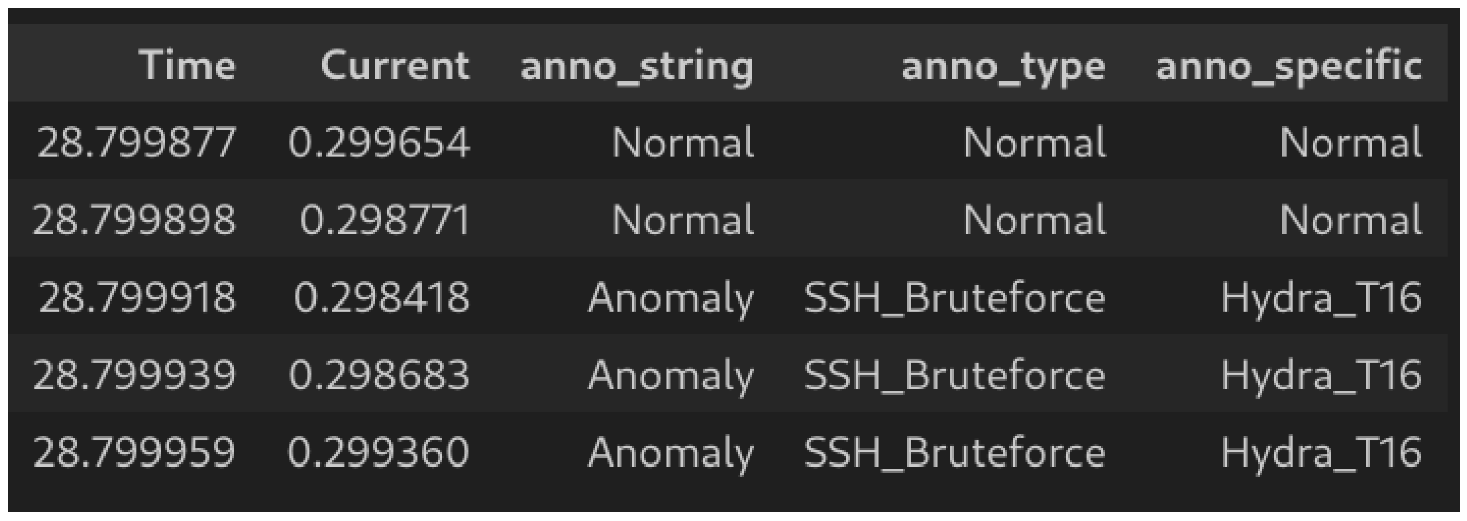
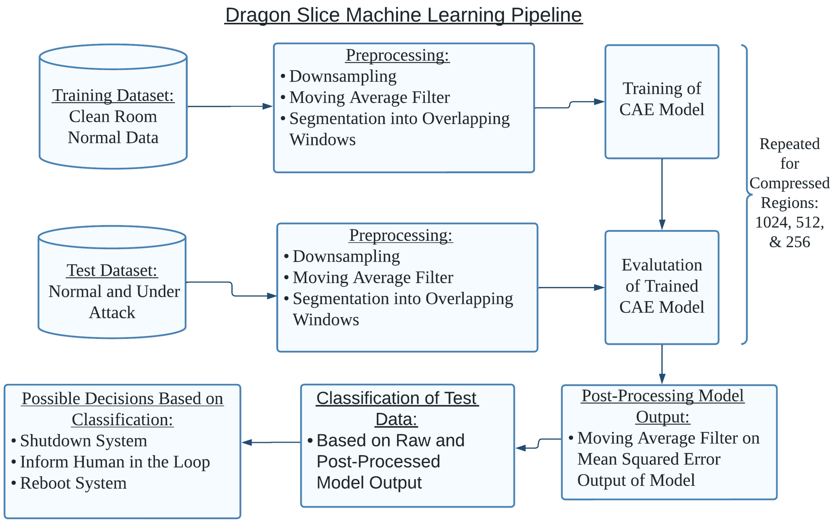


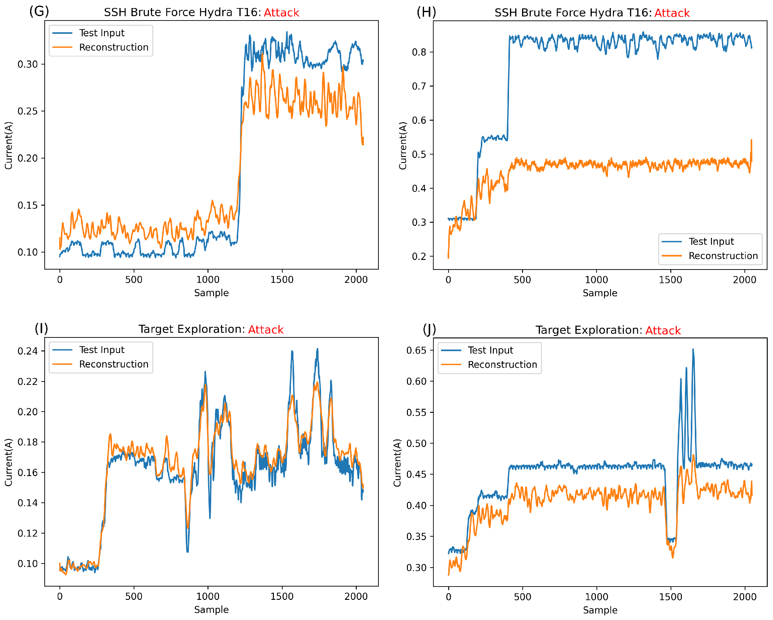
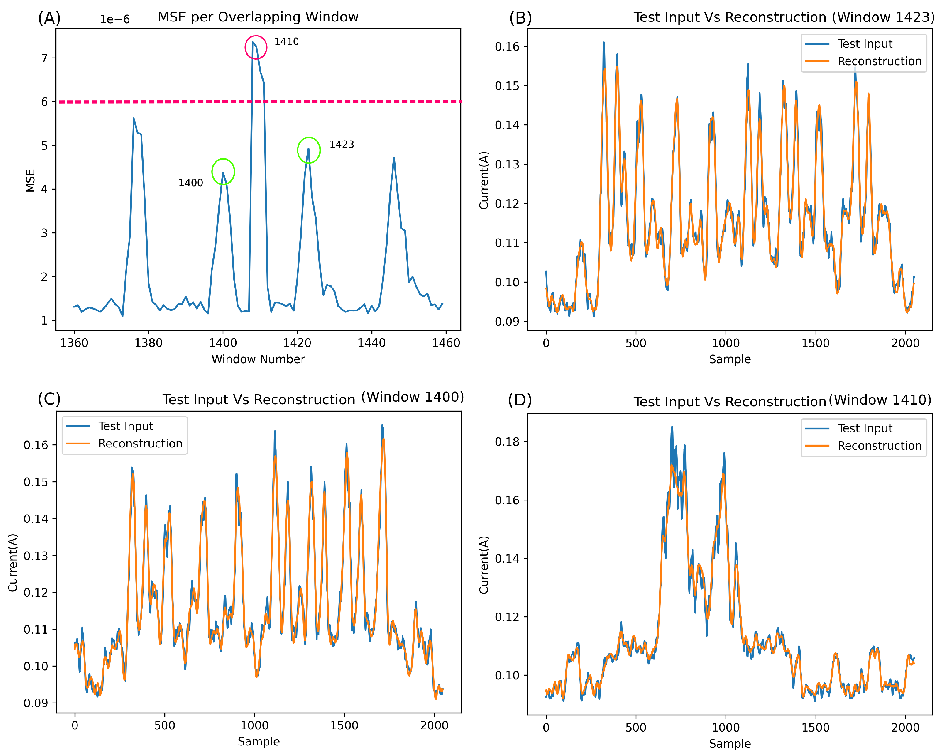


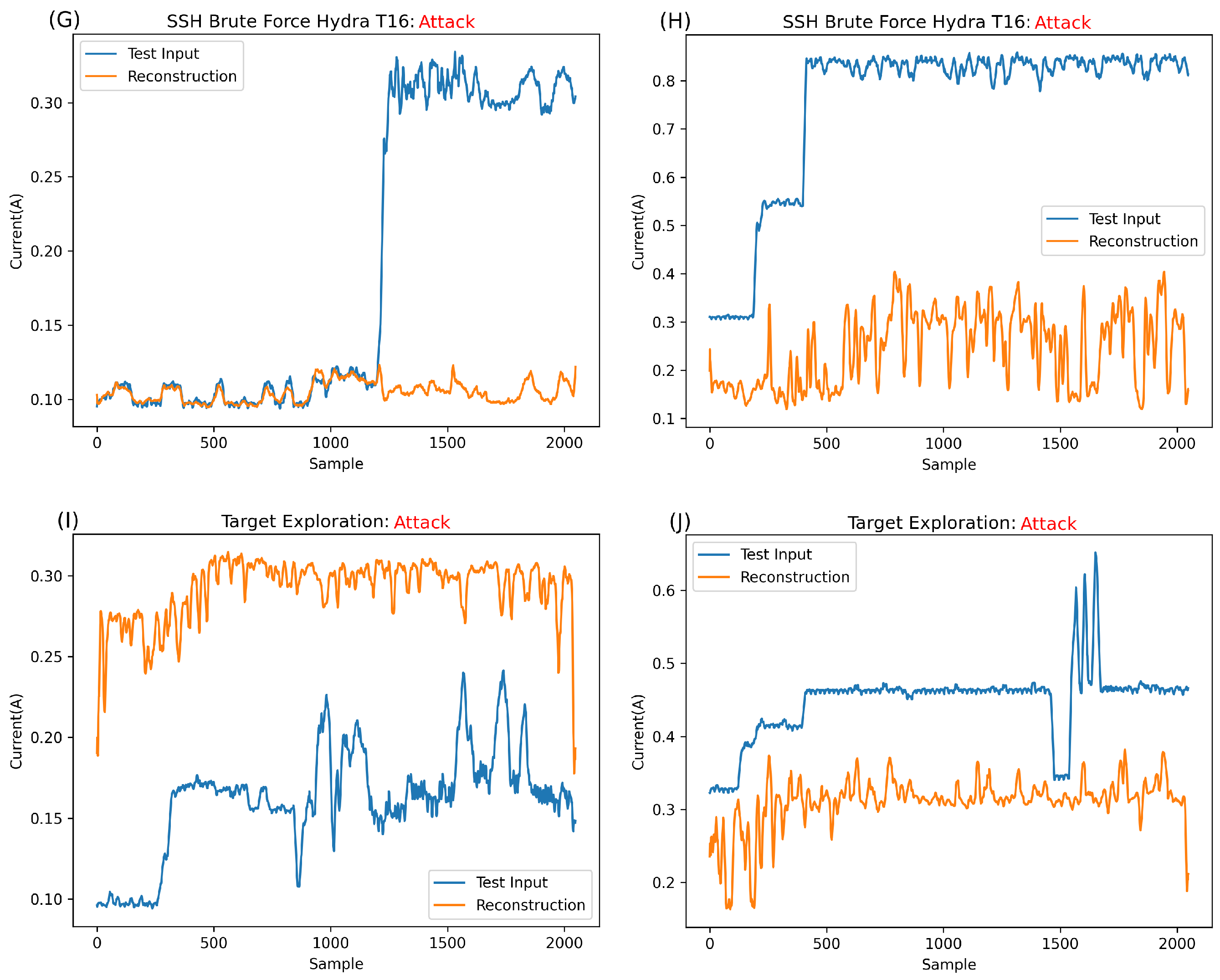
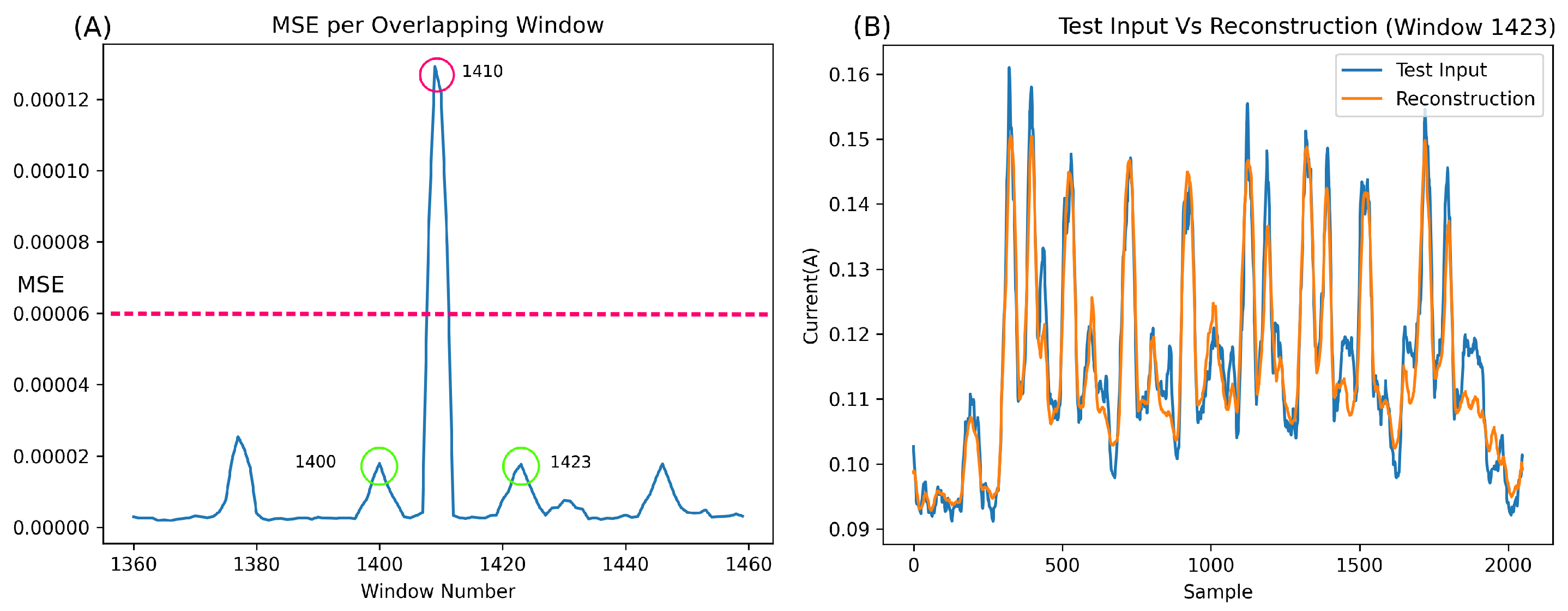
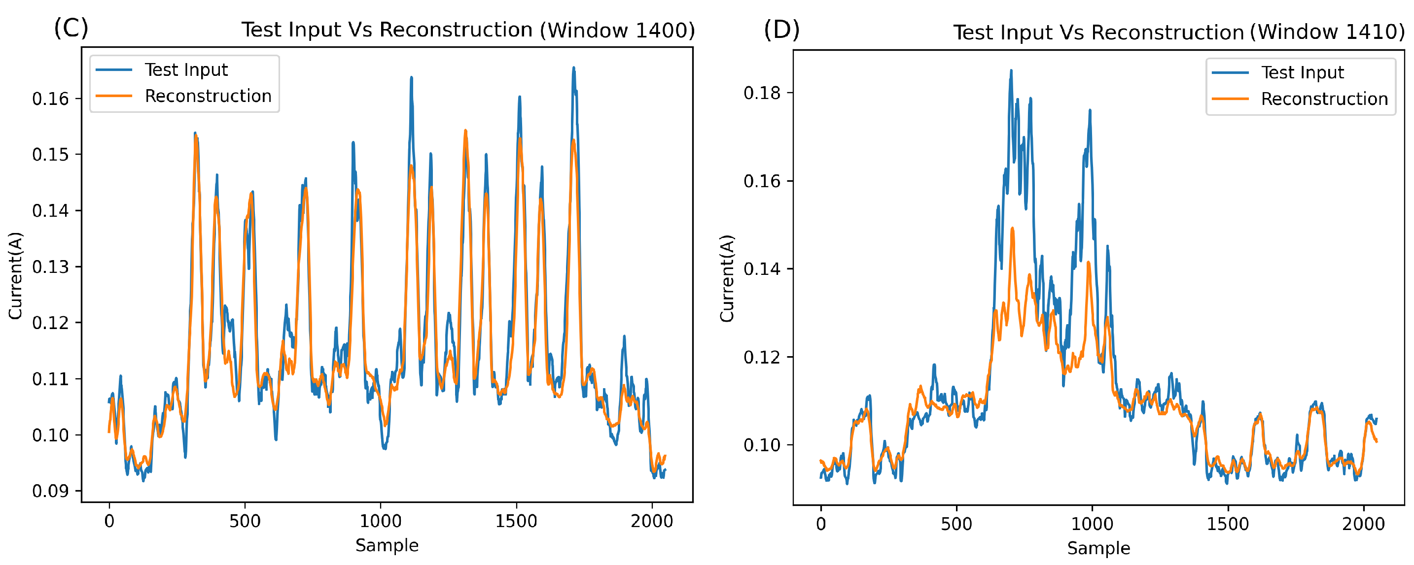


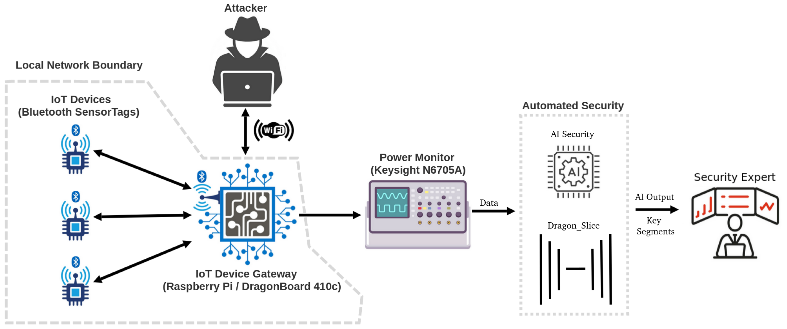
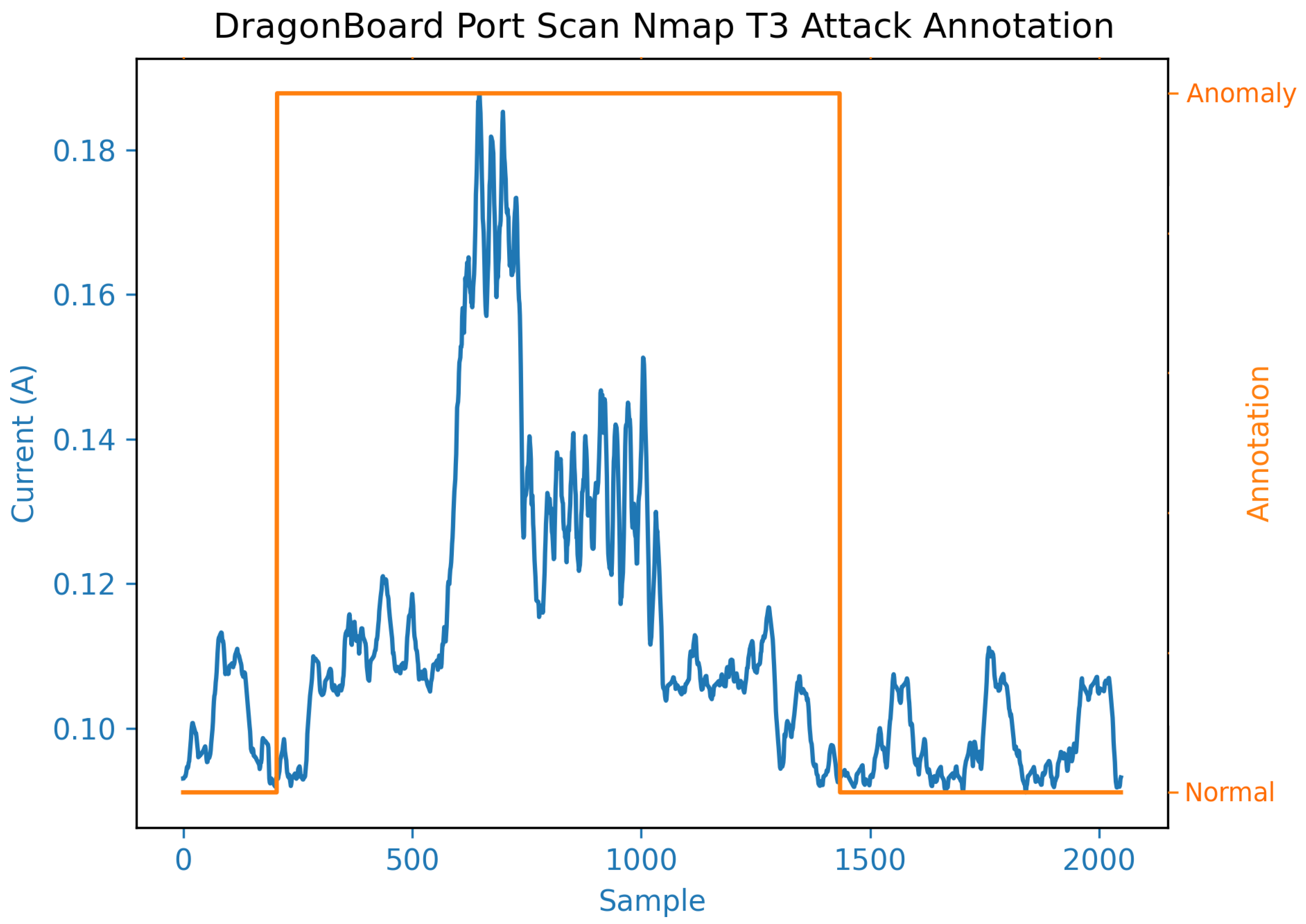
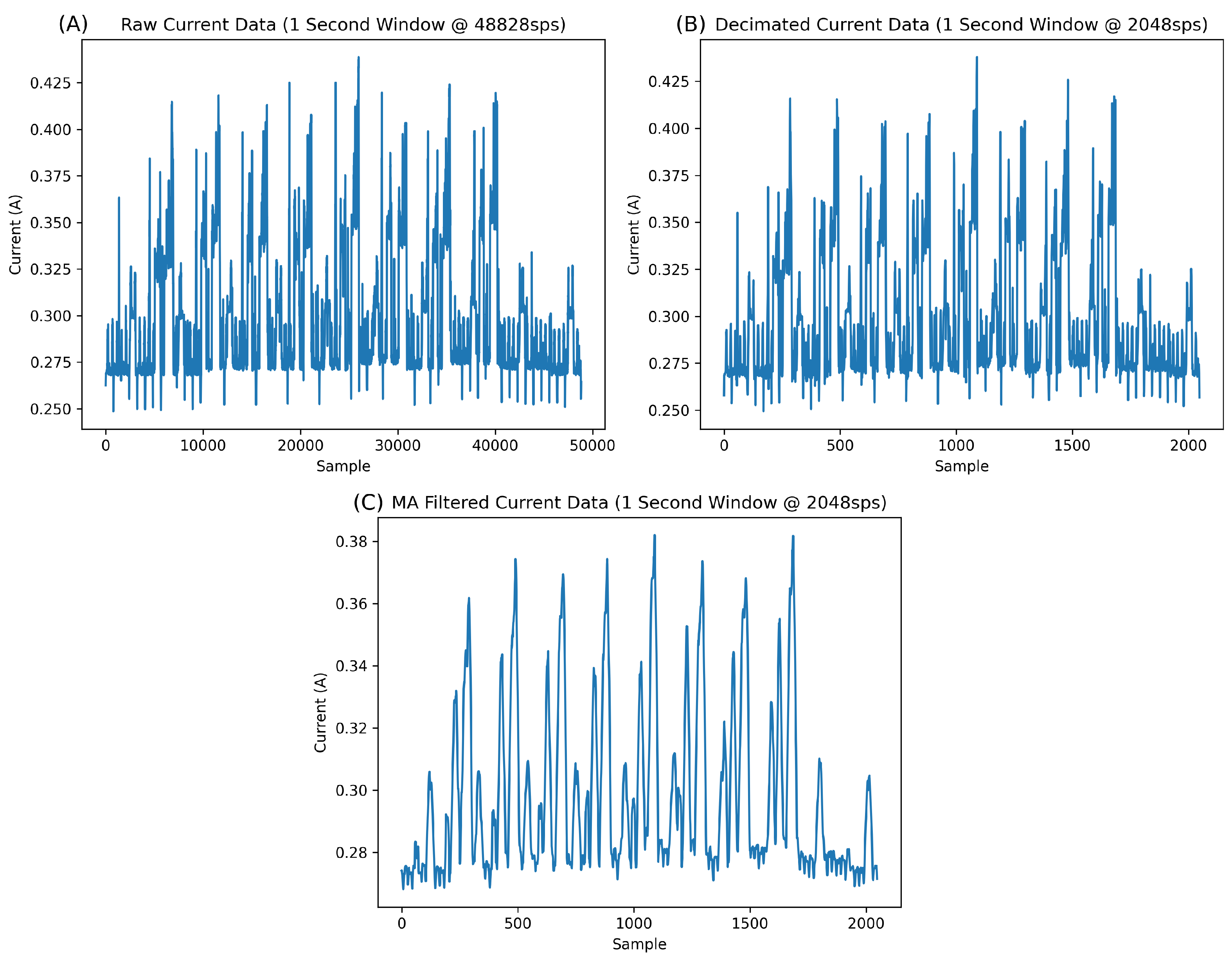
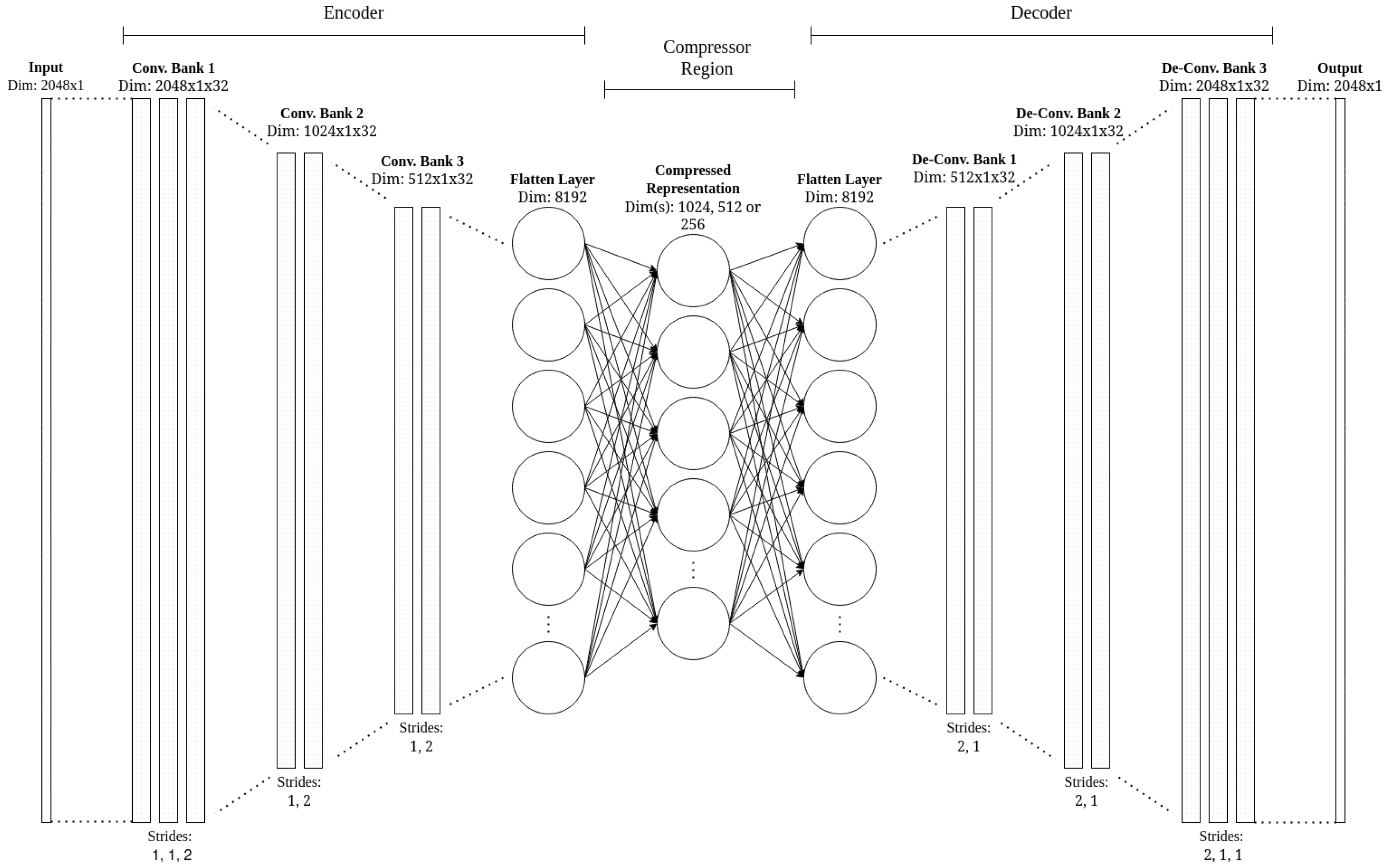
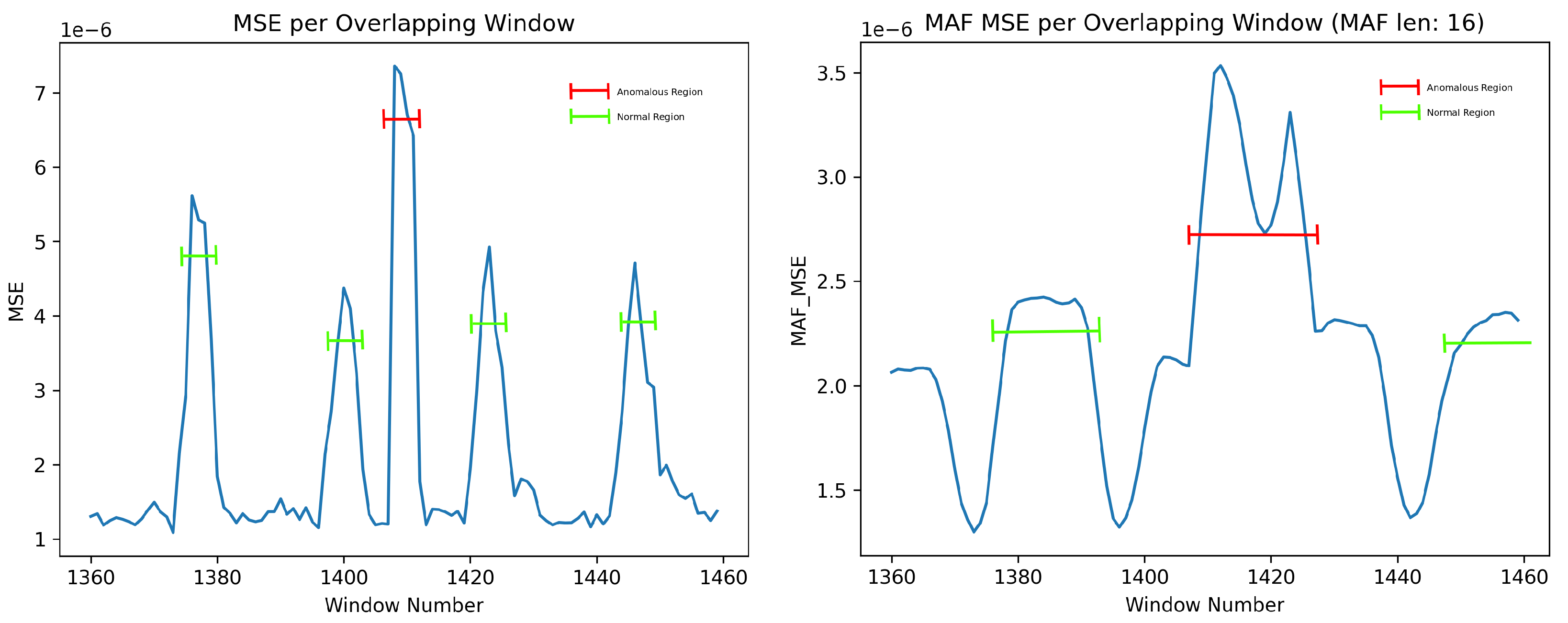
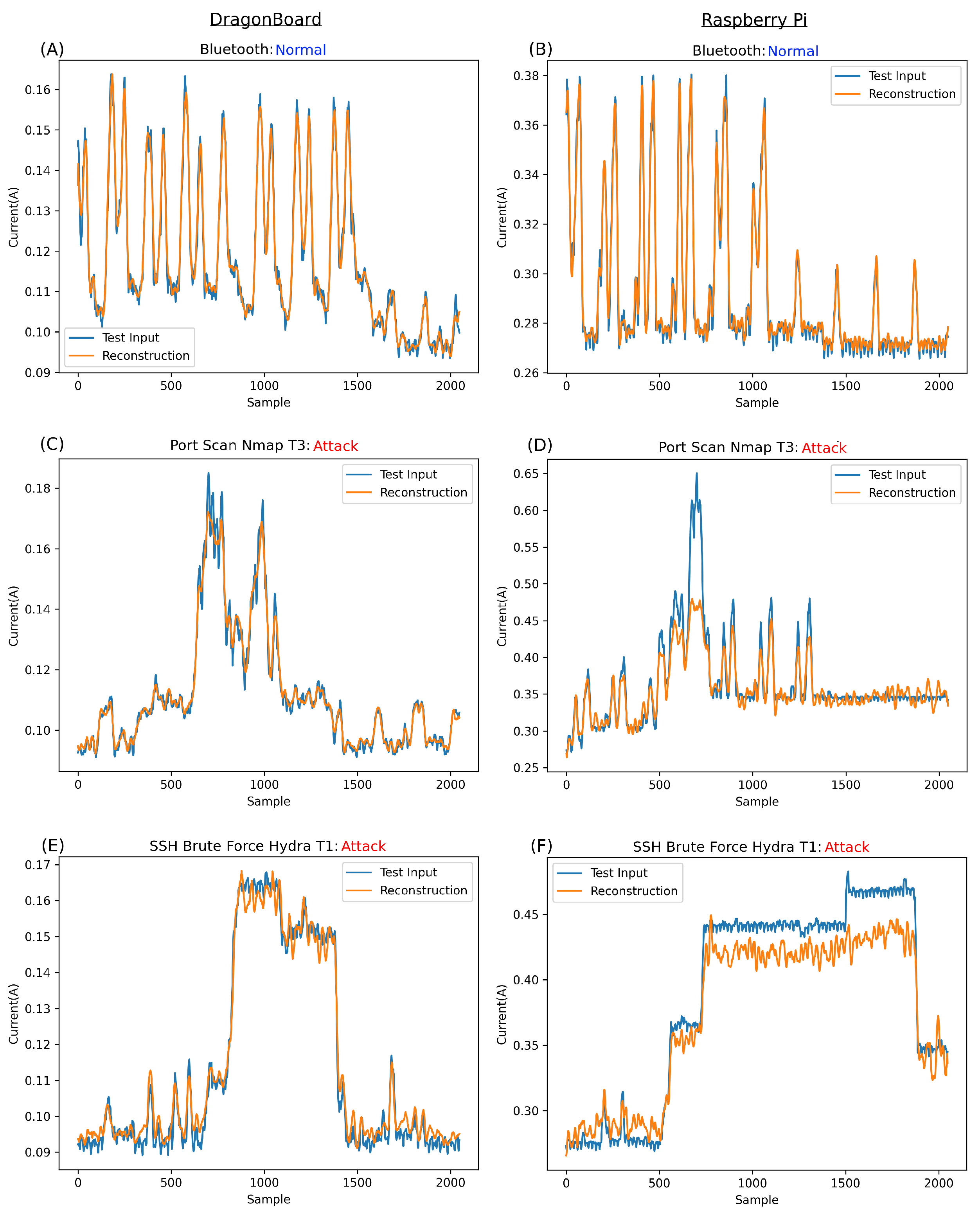
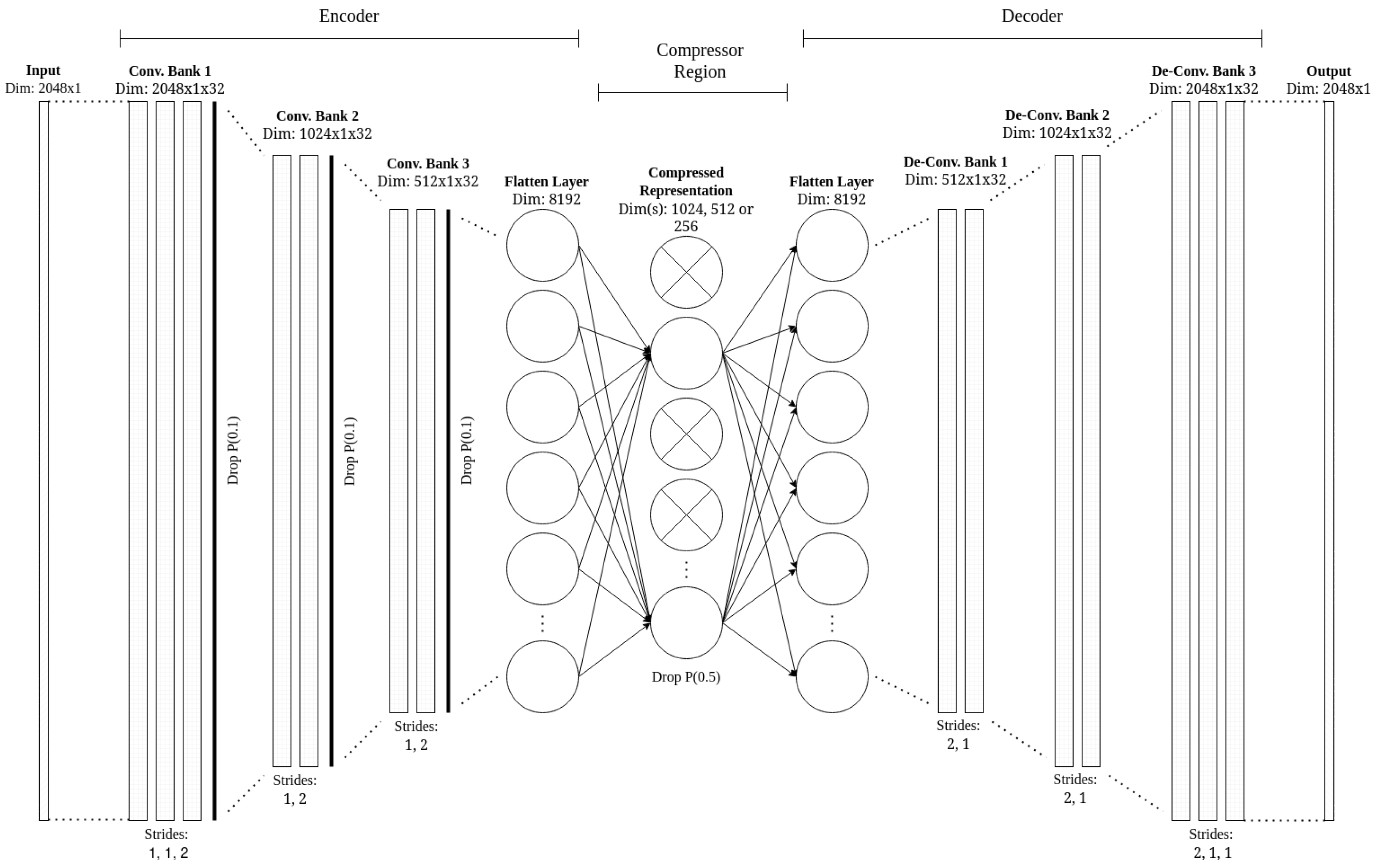
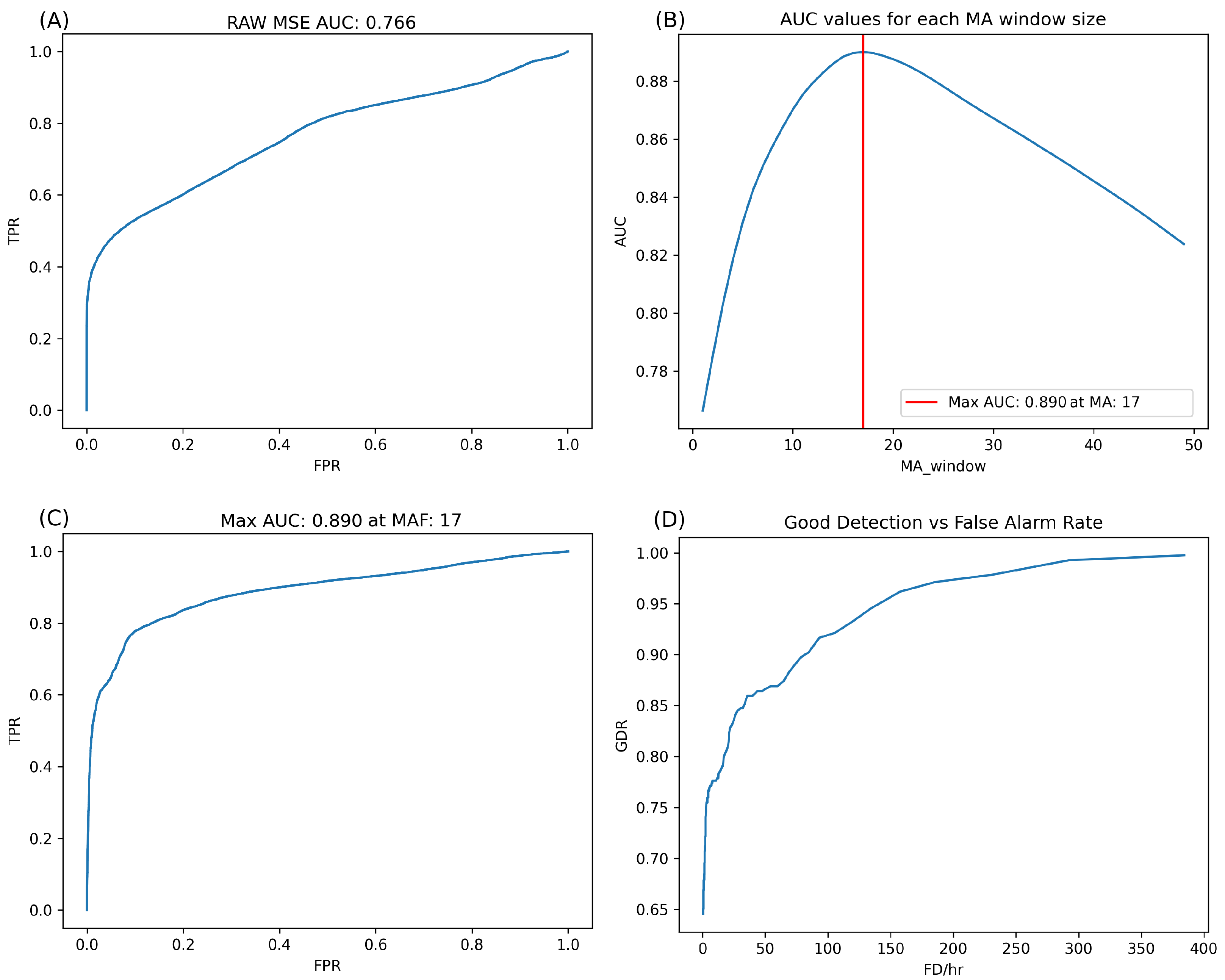
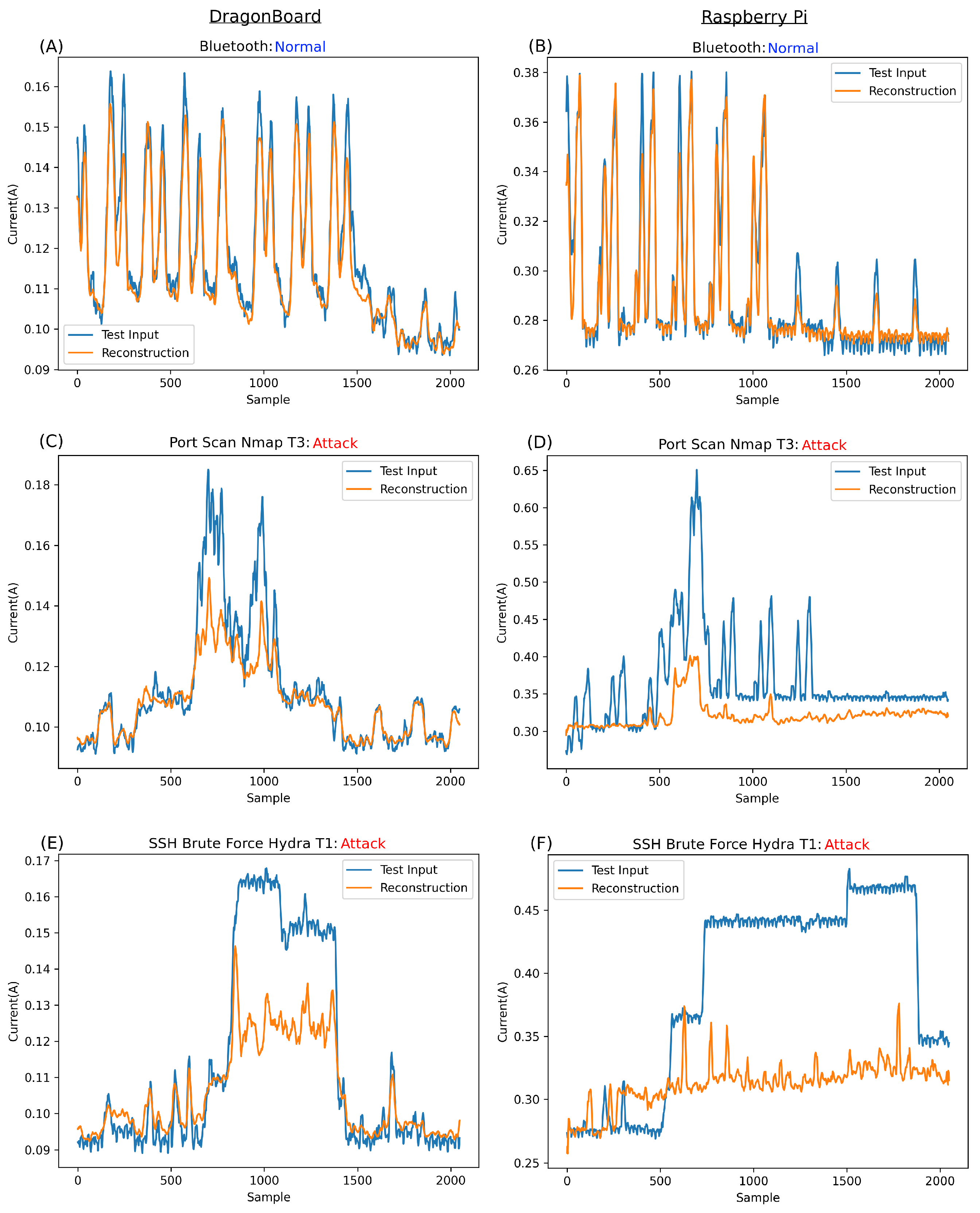
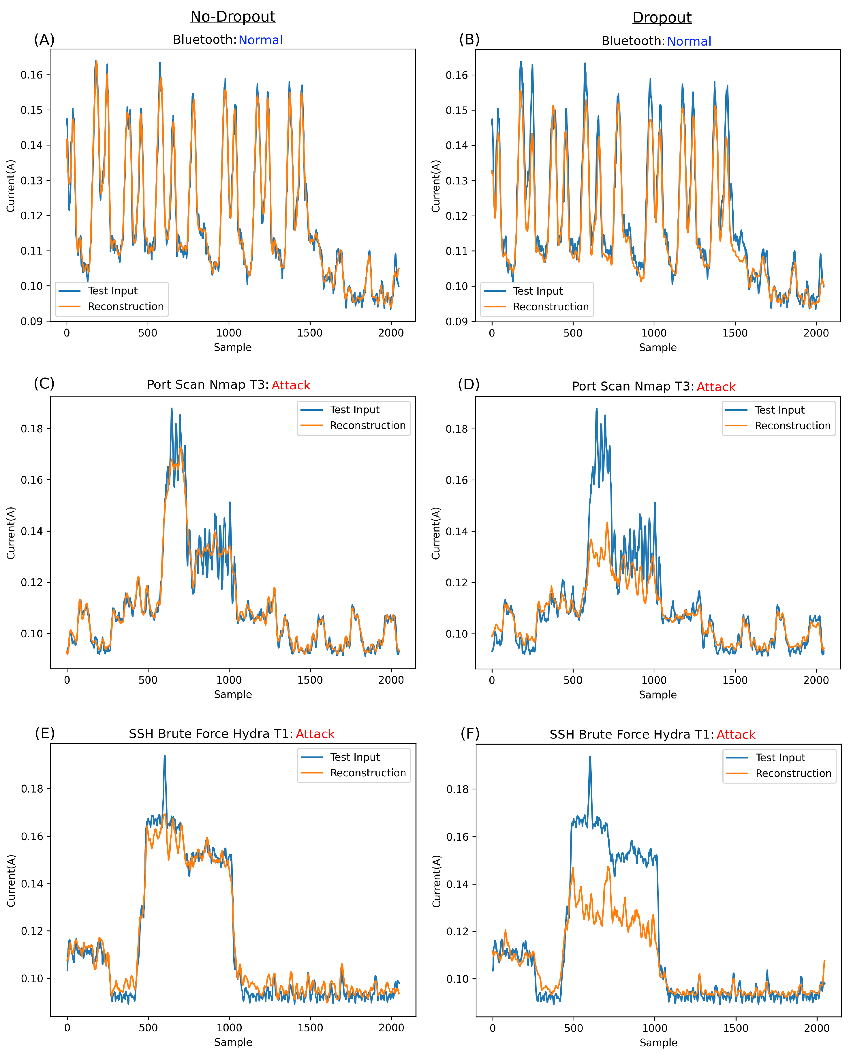
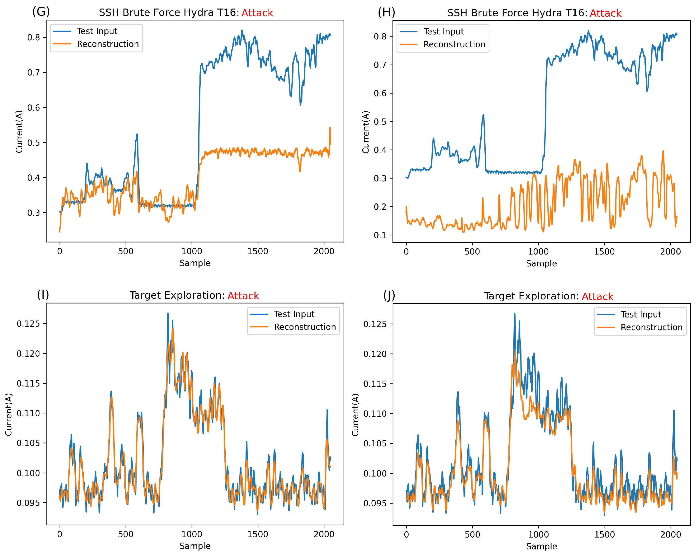
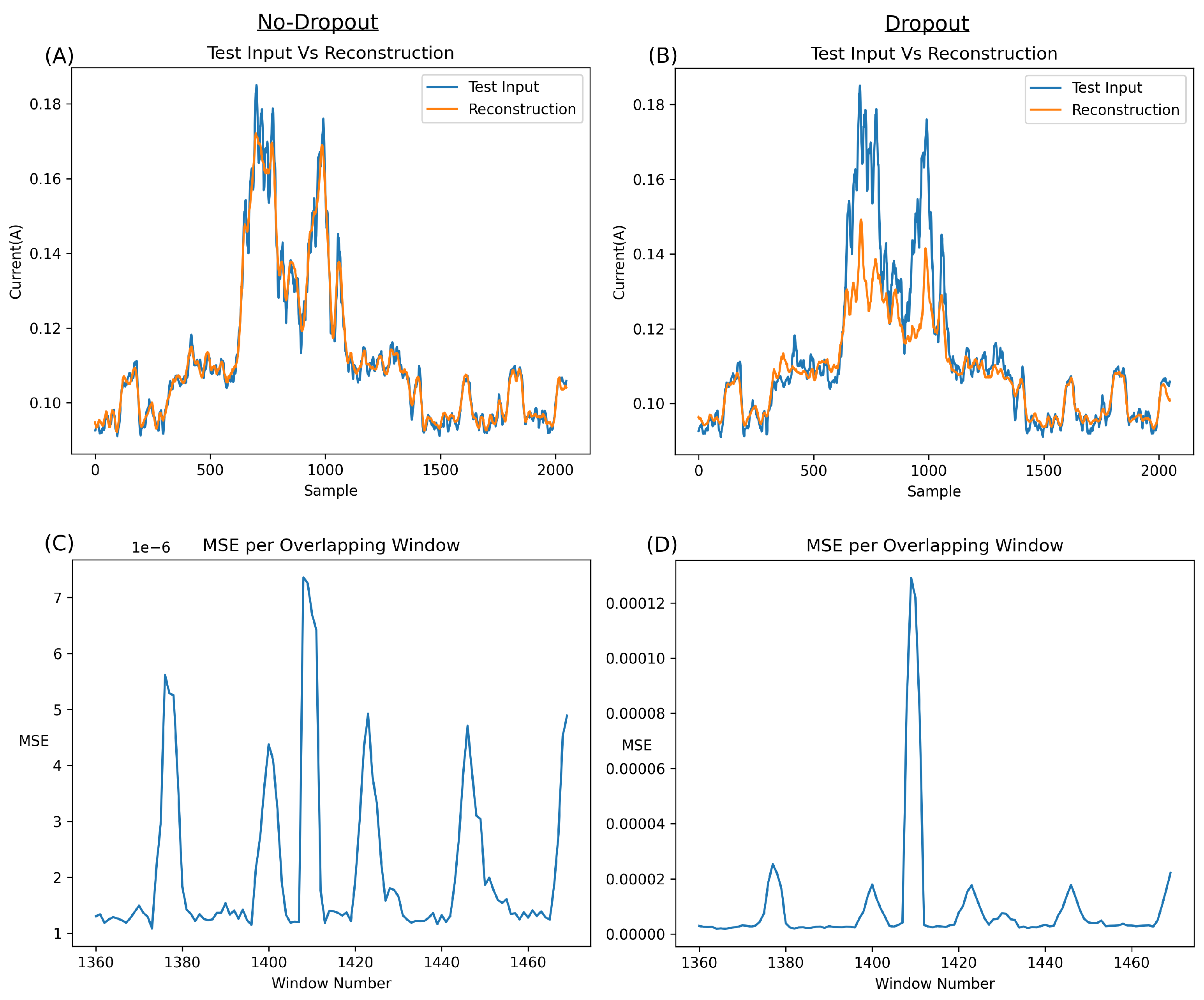