Clustering on the Chicago Array of Things: Spotting Anomalies in the Internet of Things Records

Abstract

The Chicago Array of Things (AoT) is a robust dataset taken from over 100 nodes over four years. Each node contains over a dozen sensors. The array contains a series of Internet of Things (IoT) devices with multiple heterogeneous sensors connected to a processing and storage backbone to collect data from across Chicago, IL, USA. The data collected include meteorological data such as temperature, humidity, and heat, as well as chemical data like CO₂ concentration, PM2.5, and light intensity. The AoT sensor network is one of the largest open IoT systems available for researchers to utilize its data. Anomaly detection (AD) in IoT and sensor networks is an important tool to ensure that the ever-growing IoT ecosystem is protected from faulty data and sensors, as well as from attacking threats. Interestingly, an in-depth analysis of the Chicago AoT for anomaly detection is rare. Here, we study the viability of the Chicago AoT dataset to be used in anomaly detection by utilizing clustering techniques. We utilized K-Means, DBSCAN, and Hierarchical DBSCAN (H-DBSCAN) to determine the viability of labeling an unlabeled dataset at the sensor level. The results show that the clustering algorithm best suited for this task varies based on the density of the anomalous readings and the variability of the data points being clustered; however, at the sensor level, the K-Means algorithm, though simple, is better suited for the task of determining specific, at-a-glance anomalies than the more complex DBSCAN and HDBSCAN algorithms, though it comes with drawbacks.

1. Introduction

Faulty sensors, inaccurate sensor readings, and sudden changes in sensor data in the IoT and sensor networks pose risks when utilizing these systems for monitoring and detection. Anomaly detection (AD) seeks to identify these outliers in sensor readings. In this work, we wish to test and evaluate the usefulness of the Chicago Array of Things (AoT), a large, unlabeled dataset, for the purposes of anomaly detection by utilizing clustering techniques to group anomalous readings at the sensor level.

With the proliferation of Internet-connected devices present in the market today at a low cost to consumers, from smart health devices and home devices to smart vehicles, proper anomaly detection for these devices is essential. Research in AD in IoT ranges from fault detection [1,2] to time-series AD [3,4] to malware analysis [5,6]. Many of this research points out one significant issue: the lack of available robust datasets to study AD. The Chicago Array of Things is a robust dataset from over 100 nodes, each with over a dozen sensors, spanning 4 years. The data collected include meteorological data such as temperature, humidity, and heat, as well as chemical data like CO₂ concentration, PM2.5, and light intensity. The AoT sensor network is Internet-connected; thus, it is one of the largest open IoT systems available for researchers to utilize its data. Most work referencing Chicago AoT either provides context for its creation [7,8,9,10,11], or merely references the dataset as previous work, without using it [12]. Some work utilizes a very small subset of the data [13,14] for a specific purpose, such as urban heat island detection or data cleaning.

This work is part of a multi-part analysis of the AoT. It focuses on utilizing clustering techniques at the per-sensor level and ground-truth determinations from external sources to determine present anomalies. The goal is to determine whether the AoT is viable for training and evaluating anomaly detection machine learning (ML) models. Specifically, this work analyzes independent, sensor-level clustering of the Chicago AoT using modern techniques to automate the labeling process to produce two-class anomaly labels (anomalous/non-anomalous) to train anomaly detection techniques. This work focuses on sensor-level clustering to gain a baseline understanding of the data present. By ignoring spatial and temporal contexts, we can understand how to group information in its simplest form before adding context and complexity.

The Chicago AoT is a publicly available dataset produced for general research with sensor data [8]. Its size, availability, and heterogeneity were the reasons for its use in this research. Clustering-based approaches were selected since Chicago AoT is not labeled. Due to their sheer size, manually labeling them would be time-consuming and practically infeasible. In addition, assuming the existing data are nominal and augmenting them with synthetic anomalous data may produce inaccuracies in the AD approaches, since natural anomalies may exist in the data.

Due to the sheer size of the data, the number of nodes and sensors, spatial consideration, and the time-series nature of the data, multiple different approaches using clustering and a way to unify their results are needed to determine whether anomalies exist and can be found accurately. In this work, we are focusing on clustering the data at the sensor level. We focus on the closest nodes in the dataset to the ground-truth data—weather data from the National Oceanographic and Atmospheric Administration (NOAA) Great Lakes Environmental Research Laboratory (GLERL) station in Lake Michigan [15]. These NOAA data are not used during clustering; their goal is to be used as analysis tools after the clusters are formed.

1.1. Sensor Networks

Many devices produce data. These devices contain sensors. Sensors may exist alone or coupled with other sensors. This grouping of sensors on a single device could identify a connection. Sensors in a sensor network may share similar data bounds with other sensors of the same type. This may identify another connection. Finally, sensors may be influenced by or send data to and from one another for data fusion. This may identify a third potential connection.

How you define a sensor network will determine how the sensors are connected. For instance, a person’s home may contain many IoT devices (smart televisions, smart lights, robotic vacuum, health devices, smart speakers, and utility monitoring devices). Some of these devices may naturally interact with one another (a user’s smart speaker may link all the home smart devices for a user’s control). Others may only be associated because they are on the same computer network.

The industrial IoT contains many devices working together to monitor industrial systems [16]. These systems generally report information to a monitoring system or the industrial device in case of faults or errors. The medical IoT contains many health-related sensors to notify patients and medical staff of health-related issues [17]. The environmental IoT contains devices that monitor environmental conditions, including weather and atmospheric composition [10]. This can include weather systems, atmospheric particle sensors, and light and noise sensors. The urban monitoring IoT contains devices that monitor conditions in an urban environment [8]. This can include environmental IoT, cameras, traffic sensors, counters for vehicles, people, entrances/exits, etc. Marine Monitoring sensor networks work similarly to the urban monitoring IoT, with cameras for tracking boats, but they also include ocean monitoring buoys, acoustic sensors, and various undersea sensors [18]. In all these cases, each network requires the ability to detect faults, uncommon readings that indicate uniquely sensed data, or malicious attacks. For networks that produce time-series data, anomaly detection approaches focusing on time-series data should be considered.

This work focuses on utilizing the Chicago Array of Things (Chicago AoT), a set of Internet-connected nodes along the coast of Chicago, IL. Each node in the AoT contains a set of sensors housed on circuit boards. The sensors on each circuit board are independent of other circuit boards and their sensors. This is explained in detail in Section 2. This work focuses on sensor-level anomalies, so the AoT network’s exact structure is out of scope.

1.2. Anomaly Designation

While a set of limiting thresholds can initially define an anomaly, this restriction is arbitrary and may change based on context. Various AD approaches can infer some of that context by viewing a sensor’s data concerning other sensors in the same network. To determine how to perform AD, we must first define an anomaly. This is easier said than done, as multiple sources may not agree on what an anomaly is. To clarify this, we take queues from [16,19] to specify anomalies in three ways: (a) a periodicity or temporal component, (b) a spatial component, or (c) a bounding component.

Anomaly Periodicity

Anomalies can be broken down into the following periodicities: (a) point, (b) clustered, or (c) continuous.

Point periodicity implies no period. The anomaly is seen independent of other data points. Clustered periodicity is an anomaly detected based on a set of abnormal readings compared to historical readings. Continuous periodicity is when a fundamental shift occurs in the sensor data, causing all data after a certain point in time to be markedly different from the previous data. A continuous periodicity is a clustered anomaly as time t approaches infinity. For clustered and continuous anomalies, some sliding window may be needed to identify the periods.

The sensor’s location with other sensors must be considered for anomalies with a spatial component. Techniques like graph neural networks (GNNs) [20] or R-Trees [21] can be used to incorporate a spatial context to anomalies. Concerning the Chicago AoT, the spatial component is a geo-position (latitude/longitude/altitude) that algorithms can use to determine spatial anomalies (such as urban heat islands [14] or bad air quality pockets [12]).

Furthermore, whether an anomaly has a spatial or temporal component, the basic determination of what an anomaly is relies on some understanding of a sensor’s bounds. We can look at this in three ways: (a) threshold, (b) static, and (c) lossy. A threshold anomaly is data that fall outside a bounds $\alpha$. This boundary is defined by recorded nominal data readings. These anomalies become complicated to identify when the boundaries change by time period (for example, changes in seasons) or by location (for example, sensors near a lake vs. inland). A static anomaly (or set of readings) seems “frozen” in time. A frozen reading is defined as a reading that matches (to the exact decimal) a previous reading (as far as floating point measurements are concerned). The restriction that the readings be identical is based on the tendency of sensors to have some inherent slight fluctuations in measurements due in part to things like shifting atmosphere, sensor error, etc. [22]. A lossy anomaly is an anomaly where a reading is expected at some period; however, for some reason, it was not reported. Lossy and static anomalies are related but listed here separately because they can tell a system differently. Lossy anomalies may indicate that the sensor is down due to power issues, a fault, or network access. Static anomalies may suggest a faulty or tampered sensor reading, but the sensor is still reporting lsomething.

If a dataset of sensor readings has its anomalies labeled, many common neural network techniques (MLP, SVM, random forest, etc.) can be used; however, when the data are not labeled, as is the case with Chicago AoT, to find anomalies, clustering techniques (K-Means, DBSCAN, etc.) can be used. To further complicate things, since most sensor networks produce data in a time-series format, any techniques used may need to utilize a time-series component (such as an autoencoder, LSTM, GRU, etc.) to find specific anomalies. A further breakdown of anomaly detection, defining anomalies, and the state of the art can be found in [23].

In the Chicago AoT, there are large gaps where a sensor may not produce data. For this work, since we are focusing on sensor-level clustering, these gaps are ignored, as well as any spatial context between nodes or temporal context between windows of time. This is achieved by only including the sensor readings and not their timestamps during clustering. Section 3.2 contains the detailed approach to preprocessing the data for this work.

1.3. Contributions

Our contributions to the field are as follows:

• An analysis of the Chicago AoT and its usefulness as a tool for anomaly detection in IoT and sensor networks.
• An analysis of independent, sensor-level clustering techniques on the Chicago AoT, as well as their role in labeling an unlabeled IoT dataset.

The remainder of this paper is organized as follows: Section 2 lists related work performed with the Chicago AoT. Section 3 formally defines the problem statement, the preprocessing techniques used on the data, the programming environment and tools used, the clustering approaches trained in this work, and the metrics chosen for analysis. Section 4 reports the test configuration and analysis results. Section 5 wraps up the information discovered in this work.

2. Related Work

Here, we report on the works that detail the development of the Chicago AoT, its hardware platform, and its successor projects. In addition, we focus on recent works for anomaly detection using IoT and sensor networks. For an in-depth analysis of AD in IoT, please see [23].

2.1. The Chicago AoT, Waggle, Eclipse, and SAGE

The Waggle project [7] is the hardware platform used by the Chicago AoT. Developed by Argonne National Laboratory, Waggle incorporates a modality of sensors into the Waggle platform. In addition, virtualization of edge functions was added for researchers to perform analysis and management using cloud services. The paper focuses mostly on non-environmental sensing and is more interested in computer vision and counts of pedestrians and vehicles in the wild.

This paper goes into detail about the components used in an AoT node. One computer controls the node, including sensor reading, reporting sensor data, data integrity checks, and managing security. This is only managed by system support staff, with the other computer used for edge processing. This computer utilizes the data received by the node to perform analysis. The node controller is in charge of transmitting any analyzed data. The central management server called a beehive, collects the data, registers new nodes, and manages encrypted connections between itself and the nodes. Security is handled by not allowing listening services, making the nodes fully autonomous. The Beehive only receives data from nodes and is available for interaction with system staff.

This paper points out the Waggle manager node used for managing the different computers and payloads and its robustness to failure; the AoT nodes stay working despite one or more sensor payload failures. Lastly, this paper emphasizes the need for privacy when collecting sound and video data, mentioning that the AoT nodes preprocess images before the data are sent to a cloud database.

The authors of [8] describe the AoT, its development, and the challenges and motivations for its construction. The AOT was developed with three goals in mind: (a) data analysis, (b) R&D for edge computing, and (c) R&D for new embedded hardware. These goals were determined after a series of scientific workshops. Cooperation with a city government and a modular hardware developer was needed. The city of Chicago, IL, USA, was chosen, and collaboration with Waggle, a platform designed for modularity and sensing in remote environments, began. One significant challenge and interest was privacy and usability; for the network to be viable if the Internet was lost and void of privacy issues, AoT needed edge computing capabilities to process data at the node before data were transferred to the cloud. This was performed so that audio and video were not transferred to the cloud; only the desired data from those streams were transferred (sound level and vehicle and person counts, respectively). An interesting thing to note here is that the goal of creating the AoT was not to perform anomaly detection but to provide data for researchers, a key reason for using this dataset in our research.

This work also goes into detail about the waggle infrastructure, which is a robust, modular structure allowing local data storage for situations where Internet access is temporarily unavailable, secure encrypted communications between the hardware stack and the cloud, safety management between all components of the system, ensuring the system can run when one or more sensors are down permanently or temporarily, and redundant booting in the case of a system boot failure. Since drift in sensor measurements can occur over time and re-calibration of sensors over the whole network would be costly, measurement corrections were performed on the data.

The authors of [9] reference the development of the Chicago AoT. This paper specifies that SAGE is the successor to Chicago AoT, an NSF-funded collaborative project. It further elaborates on the Waggle platform like previous papers have carried out. The work seen in [10] is a similar product to Chicago AoT and another successor project. This paper notes that many air sensors in the AoT dataset were susceptible to hardware failure during transport. So, rather than replace the entire node when other sensors were working on it, they left the nodes in place, allowing the remaining functional sensors to report data. This paper evaluates a new modular, low-cost air quality sensing hardware platform called Eclipse. This paper only compares to the AoT and focuses more on a new hardware platform than on utilizing AoT data or Anomaly detection. Catlett et al. in [11] write a documentation of the history of Chicago AoT and mention SAGE as its direct successor. This work identifies in more layman’s terms the processes by which AoT and SAGE came to be and the reasons for doing so. This paper points out that the AoT Team collaborated with The Eclipse team to deploy the Eclipse sensors mentioned in [10].

2.2. Recent Advances in Anomaly Detection (AD) on IoT and AD Using Chicago AoT

In [24], Asanka et al. focus on utilizing multi-agent systems (MAS) and time-series AD techniques to detect unusual human movements. The dataset utilized involved mobile phone data. The time-series data were determined to be non-stationary using the Dickey–Fuller technique, then converted to stationary using the min–max technique. Part of their approach involved filling gaps in missing time-series data. They completed this by utilizing a simple rule (fill in 0 s if there are 0 s previously and ahead) and regression using root mean squared error. Boosted decision tree (BDT) regression was chosen for outlier detection. Seasonal trend decomposition was used.

In [25], the focus is on finding faults in etching equipment used in Tool-to-Tool Matching (TTTM) in semiconductor manufacturing. Their approach focuses on rapid gradient shifting and deviations from the normal trend range. The first algorithm is called the gradient drift detection algorithm (GDD). The approach relies on the interpolation of missing data and relies on a median value for determining the sensor range using bins of data. The gradient of the data is found by differencing these median values. Rapid change detection is performed using algorithms like Isolation Forest. The second algorithm is called trend zone detection (TZD). A trend line is calculated between the data, smoothed, and adjusted. A plane model like an SVM is used to detect deviations.

In [13], English et al. focus on how the environment, particularly air quality, affects personal health. It utilizes two datasets: the Chicago Health and Real-Time (CHART) project, which contains health and daily activity impact on elderly Chicagoans, and the Chicago AOT’s air sensor data. CHART collects GPS data and surveys on willing participants to determine activity and health. This work points out that 80% of CHART participants lived within at least one AoT node, so the overlap between datasets is viable. Previous studies were used to determine the ground truth of the AoT air pollutant data to determine the minimum and maximum levels for certain gasses by checking if the AoT node exceeded the highest or lowest values or where humidity was lower than 0 or higher than 100%. In addition, any data points with less than 10 months of temp and humidity data available were excluded from annual averages. To generate averages over the area, inverse distance weighting over a 200 m × 200 m grid was utilized, and mean values within 250 m of a CHART participant’s address were used to determine exposure. Correlation between gasses was performed, and any highly correlated gasses were removed in favor of the known “criteria air pollutants” they were correlated with.

Logistic regression models were fit based on the binary surveys performed by CHART respondents using the Hosmer–Lemeshow test. To test the improvement of the fit using the AoT data, likelihood ratio tests and Akaike’s and Bayesian information criteria were used. Three models were used. The first model utilized air quality and weather conditions. The second model was an individualized model based on surveys of health, demographics, and length of time in the area. The last model combined the two to determine short and long-term effects.

Notable results were that the air quality measurements in the area only affected respiratory health in long-term residents, particularly due to higher levels of $N{O}_2$, and that while air pollutants do negatively affect overall health, due to the correlation between the different pollutants, it is unclear which specific pollutants are the most egregious. In addition, this work points out that when AoT data are compared to EPA data on air pollutants for the area, an unknown amount of measurement error may have been introduced due to the low-cost nature of the sensors in the AoT nodes.

One thing to note here is that this work does not focus on anomaly detection, but rather the general usefulness of the AoT data, as well as how to correlate the data with themselves and ground-truth measurements from outside the set.

The work in [12] utilizes time-sliced anomaly detection (TSAD) to discover spatial, temporal, and spatial–temporal anomalies in segments of a large-scale sensing system. This work utilized the AirBox dataset (out of Taiwan) to determine anomaly detection for air pollutants. This work defines spatial, temporal, and spatio-temporal anomalies. TSAD determines spatial anomalies using Tukey’s test, a temporal anomaly if data fall out of a reasonable measurement drift. Spatial–temporal anomalies are determined if both occur.

Once this is completed, the results are fed into three other components: ranking, emission detection, and malfunction detection. The ranking is used to determine how well the device is performing, emission detection is used to determine, in real-time, the air quality based on the anomalies seen, and malfunctioning devices if extreme values are seen very often. This is essentially a set of heuristic or meta-heuristic tests, rules that may or may not assume certain criteria must be followed. In addition, no comparison against other methods was performed. While this work references Chicago AoT, it does not perform AD work with it.

The driving factor for [14] is the danger of and necessity to eliminate urban heat islands, a human-made condition where areas of urban development experience extreme heat events. To facilitate this, this paper employs tensor factorization to impute missing values and correct errors in sensor network data. This study uses the Chicago AoT dataset, and NOAA data are used to compare and determine the ground truth. To do this, Tucker ranking, nuclear and L2 norms, singular-value thresholding, and the alternating direction method of multipliers framework were used in the factorization. The result was an output free of outliers and contained complete (though imputed in places) data. This work focuses on cleaning the data for analysis rather than generating a model that finds anomalies, though it does seem to produce an anomaly tensor ($ϵ$). Exactly how these tensors are created is not detailed in this paper. In addition, the focus was on removing the outliers, not determining whether they provided anything of import.

The work in [26] utilized satellite data and the Chicago AoT to predict urban heat islands, where the temperature is significantly hotter than other portions of the city due to lack of green space, shade, or less circulation. This work performed linear interpolation on the bi-weekly satellite data to obtain daily data. For ML algorithms, random forest regression (RFR), artificial neural network/multi-layer perceptron (ANN/MLP), support vector machine (SVM), and polynomial regression were used. Mean squared error (MSE) and mean absolute error (MAE) were used to evaluate model performance. This paper also details how the data were processed, an important step in beginning an ML analysis. The data were filtered by location and time; then, the data were collected in 10 m time-series windows, reduced to an average value over that window, and anomalies were removed based on temperature values that exceeded some sensor boundary or predetermined cutoff value (rules-based AD). Other AD methods are performed on the same sensors on the same node to find outlier cutoff values. To do this, quantiles determine an upper and lower bounded “fence”. Again, this is a rules-based AD. The valid data from similar sensors are then averaged again to produce a single attribute value to be used. To deal with missing values in the data, multivariate imputation by chained equations was used [27].

For convenience, a summary of these approaches can be seen in Table 1.

Table 1. Summary of approaches reviewed.

Citation	Goal	Dataset	Approaches	Notes
[24]	unusual human movement detection	phone position	BDT regression, Seasonal Trend decomposition	uses last-value imputation
[25]	fault detection	T2T manufacturing	GDD, TZD,SVM	uses mean imputation
[13]	personal health and environmental factors	CHART, Chicago AoT	gridding, correlation, logistic regression	focuses on correlation, not anomaly detection
[12]	AD in sensors	Airbox	TSAD,Tukey’s test and reasonable measurement drift	utilized heuristics/metaheuristics for AD
[14]	prediction of urban heat islands	NOAA (ground truth), Chicago AoT	tensor factorization	removing of outliers (not detection explicitly), imputation was used
[26]	prediction of urban heat islands	Satellite Data, Chicago AoT	AD using quantiles, prediction using RFR, MLP, SVM and polynomial regression	rules-based AD, removal of outliers for prediction, rather than detection

3. Methodology

We aim to study the usefulness of clustering approaches on the Chicago AoT to determine its usefulness for anomaly detection. Clustering was chosen since the Chicago AoT is not labeled. The goal is to build a mechanism by which we can auto-label the dataset. We focus on sensor-level clustering in this work. For this work, we are focusing on three available clustering methods:

• K-Means: The baseline clustering algorithm.
• DBSCAN: A modern clustering algorithm.
• Hierarchical DBSCAN: A modification of DBSCAN that utilizes tree hierarchies in its clustering.

Each clustering tool was chosen for its popularity and usefulness.

3.1. Problem Statement

More formally, we define the problem here: Definition—Given a sensor dataset S of dimension d, we aim to discover anomalies in S utilizing clustering algorithms. The following expression can formulate that:

$$S^d=>C\left(S^d\right)=S^{d+1}|S=S_{n-m}\cup S_m$$

(1)

where n is the total number of records in S, m is the number of anomalous records in S, C is some clustering algorithm acting on S, and the $d+1st$ dimension in S represents the anomaly label. Specifically, we aim to analyze various clustering algorithms on an unlabeled sensor network dataset to produce a labeled dataset that can be used to train deep learning techniques to perform more accurate AD in sensor networks as readings arrive at the sensor. In this work, we focus on sensor-level clustering, treating each sensor on a node as independent to determine the anomalies specific to the sensor.

3.2. Dataset Preprocessing

Each record in the Chicago AoT dataset is a single sensor reading from a single node at a single point in time. Each node (over 100) reports all of that node’s sensor readings periodically, around every 30 s. See Figure 1 for an example.

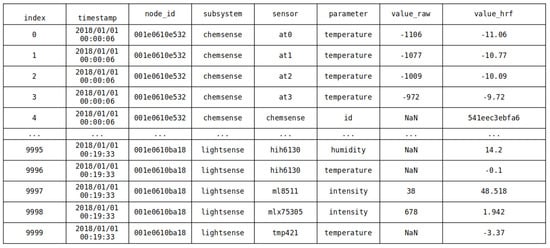
Figure 1. An example of the AoT data.

The first step is to prune the data that are irrelevant to the types of anomalies we are interested in. The AoT records everything, from internal sensors used to manage the thermal safety of computer parts to network logs to environmental data. The system-level management logs are out of scope for our work, so they are removed from the set. This reduces the size of the dataset and will speed up the processing of the data somewhat.

For data processing, the type of clustering that is to be performed needs to be defined. Here, we specify three separate clustering paradigms: (a) node-level clustering, (b) spatial clustering, and (c) temporal clustering. For this work, we focus on node-level clustering, specifically sensor-level clustering on each node.

Node-level clustering is the process of determining, at the node level, how the sensor data can be clustered. We treat each sensor as independent and ignore the time component entirely or treat the timestamp as one of the feature vectors in the clustering algorithm. For spatial clustering, sensor readings from neighboring nodes are taken into context to determine whether the sensor readings show any localized phenomena. Temporal clustering allows us to break whole sensor readings into windows to determine trends. This allows us to determine whether the sensor readings are nominal for the time they are recorded or whether some temporal phenomena have occurred. Lastly, properly merging these three approaches together will provide us with more context of anomalies occurring in the AoT. For this work, we focus on the independent sensors in node-level clustering due to the size of the dataset and to obtain a baseline to enhance future multi-dimensional node-level, spatial, and temporal analysis. Specifically, we utilize the one-sensor-per-row format native to the Chicago AoT and independently cluster each sensor and node. This produces multiple results for labeling per node but allows us to analyze the performance without considering the effects other sensors in a node would have on a result.

With this in mind, the dataset should be filtered by node ID for easier processing and management. We can also visually inspect the readings of certain environmental sensors and reference them against any ground truth we have available. We utilize local NOAA weather data (temperature data) for this work. The NOAA data are available for public use [15] and will act as our ground-truth reference.

By plotting the NOAA data against each Node ID’s temperature data, we can visually (or through heuristics) determine some anomalous data. Since the NOAA data are only for a specific point in the area and the AoT spans miles along the shore of the lake and some interior of the city of Chicago, this only gives us a partial understanding of what each node is seeing. In addition, the NOAA data only provide us with ground truth for some of the sensors on a node. Therefore, we must decide which data (if any) to prune, how much of the remaining data to use as feature vectors, and how (and whether) to normalize these data.

Since each node has the potential to be heterogeneous, some nodes may have more or different sensors than other nodes. In addition, since the distance to the NOAA station varies from node to node, we limit the number of nodes to those closest to the NOAA station with similar sensors. We also focus on temperature data as comprising a further limiting factor without normalizing the records. For an example of the nodes in question, please see Figure 2. The left side of the figure represents the zoomed-out location of the nodes off the coast of Lake Michigan. The right side of the figure is the zoomed-in representation, where you can make out individual sensors.

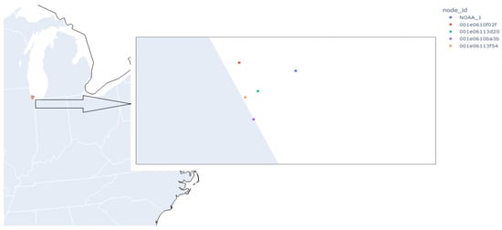
Figure 2. The data subset focused on for this work.

Lastly, many works, such as [14], incorporate imputation into their analyses. Imputation is the process of filling in gaps of missing data. This helps reduce sparse matrices generated when some sensor data are missing or if generalizing an entire dataset of heterogeneous nodes into a set that contains all sensors for all nodes on each row, where rows corresponding to nodes that do not have those sensors are filled in with some sentinel value. Unfortunately, while imputation allows the data to be more easily digested by various algorithms, it has the downside of potentially biasing the data [28]. As such, we do not impute data.

We treat each sensor separately for node-level clustering, running clustering algorithms on each sensor type for a given node. Normally, this would be time-consuming, but due to the available hardware, the spark module for accessing data, and the steps we took to process the data for this analysis, the run-time for the clustering algorithms was reduced significantly. The result was around 800,000 records per sensor, and we focused on the 4 nodes closest to the NOAA data, with each node containing 5 sensors for approximately 16 million data points. No individual records for the sensors used in this research were removed from the dataset.

3.3. Algorithms

The K-Means algorithm was first introduced in [29]. It is closely related to Lloyd’s algorithm in [30], which generates Voronoi diagrams and was originally created for pulse–code modulation. In K-Means, k random points are chosen as centroids of the desired k clusters. The distance from each remaining point is then calculated between the centroids. After all points are assigned to exactly one cluster, the centroid is then calculated again. The process continues for several steps or until points are not re-partitioned. The distance calculation used is the Euclidean distance (or $L_2$ norm).

The K-Means algorithm is simple but effective. However, it is not guaranteed to obtain globally optimal clusters. For a more detailed description of K-means, please see [29].

The DBSCAN algorithm was introduced in [31] and relies on clusters based on density rather than distance to a centroid. Multiple definitions are used to define density in [31], but the core rules are as follows:

• A single parameter, $minPts$, is used to determine density. This determines the minimal number of points any other point is density-connected to.
• Density connectivity: a point is density-connected to another point if there is an unbreakable chain of points from p to q; here, each point in the p-q chain is, at most, $ϵ$ apart in distance.

DBSCAN then merges clusters that are close to one another. This is performed by finding the smallest p-q distance where p is in one cluster and q is in another. The clusters are merged (i.e., combined to form a larger cluster) if this smallest distance is <= $ϵ$.

The benefits to using DBSCAN over other methods are it does not rely on defining the number of clusters, the distance calculation can be different (unlike K-Means, which generally requires $L_2$ distance), and the number of parameters to test is reduced to 2: $ϵ$ and $minPts$. These hyper-parameters are global. The values can then be chosen through evaluation or a heuristic posed in [31] relying on distance from an arbitrary point p to its k-nearest neighbors. For a more detailed description of DBSCAN, please see [31].

Hierarchical DBSCAN (H-DBSCAN) is introduced in [32]. It is a variation of DBSCAN and relies on a minimal spanning tree (MST) to generate a hierarchy for more advanced clustering. To generate this hierarchy, a new metric, the mutual reachability distance, is the maximal value of the core distances ($ϵ$) of points p, q, or the distance between them. In contrast to the original DBSCAN algorithm, rather than merging clusters close together, H-DBSCAN starts with one cluster and uses the MST to split clusters off by sorting the MST by edge distance and splitting points off that match edge values. A new cluster is formed if the points split off have at least $minPts$. This process iterates until all points have been split from the MST. Each new cluster keeps a reference to its parent cluster.

From here, a stability value can be generated for each cluster. The stability of a leaf cluster (a cluster with no children) is compared against the stability of the parent cluster. If the child’s stabilities are higher than the parent cluster’s stability, these stability values propagate to the next parent until root. Otherwise, the parent cluster’s stability propagates. In this way, there are no multiple clusters representing the same point. H-DBSCAN can also specify outliers in the data using information calculated for each point as the point was being placed into a cluster. For more information, a detailed description can be found in [33].

3.4. Metrics

Since we are looking at node-level clustering in the context of binary anomaly detection (a reading is or is not an anomaly), and since we are considering all of a node’s sensors independently to determine the cluster the reading falls into, we will determine the efficacy of the techniques based on whether the NOAA ground-truth visual analysis confirms a reading was an anomaly or not; if so, we ask the following question: does the cluster group in a way that verifies this (and by measuring the Davies–Bouldin Index of the clusters)?

The first criterion is straightforward: given a readout of NOAA data for the given period and the weather sensor reading for the same period, are readings significantly different than the NOAA data clustered together? The term “significantly different” is subjective, so here, we define it as the mean value of the difference between the sensor reading and the NOAA reading in the same time frame. We detail how we find the closest value for a given sensor reading in Section 3.5.

The Davies–Bouldin Index (DB Index) was introduced in [34]. It is an internal cluster evaluation scheme that uses quantities and features inherent in the dataset. The DB Index is calculated by finding the maximal value based on adding the individual distances within a cluster (intra-cluster distance) i and every other cluster in the set and dividing by the distance between these clusters (inter-cluster distance), then summing up all the values for all combinations of clusters and dividing by the number of clusters. The lower the value, the better the result. The drawback of this method is that a good value reported by this metric does not necessarily guarantee the best information was retrieved. The DB Index is available in the standard Python sci-kit learn package and in [35]. Please see [34,36] for an in-depth description. In brief, the DB index acts as a measure of the closeness and density of the clusters.

$$DBIndex\left(U\right)=1/k\sum _{i=1}^k\underset{i\ne j}{max}\left\{\frac{\Delta \left(X_i\right)+\Delta \left(X_j\right)}{\delta (X_i,X_j)}\right\}$$

(2)

3.5. Testing

Here, we focus on node-level clustering; each node in the AoT is treated as a separate, independent entity without contributing meaningful information to the other nodes. By restricting our clustering, we can gain a baseline for how individual nodes in the AoT see the world and pick up node-level anomalies. Due to the number of nodes in the set, we chose $n=4$ nodes in the dataset and performed clustering on them. The following procedures will be observed:

• Temperature readings will be used to heuristically infer anomalies in the data when directly compared to NOAA data. This comparison will be performed per the mechanisms seen in Section 3.4.
• A node’s sensor data will be pruned only to have relevant sensor information present. Reports such as network uptime, individual component IDs, a sensor’s location, etc., are outside the scope of this paper.
• A comparison using the DB Index listed in Section 3.4 will be used to determine the efficacy of the clustering algorithms. Again, the lower the score, the better the clustering.

The four nodes chosen (f02f, 3d20, ba3b, 3f54) can be seen in Figure 2. The data for these particular nodes span 2 years (2018–2019). We collected the relevant NOAA data, which were collected from the NOAA GLERL Met Station at Latitude 41.78, Longitude −87.76, just off the coast of Chicago, IL, USA, in Lake Michigan. The NOAA data are not used as part of the clustering algorithms but only to compare clustering success.

Each node utilizes the same five Metsense sensors: bmp180, htu21d, pr103j2, tmp112, and tsys01. Each of these sensors was part of the node’s meteorology sensing stack. These specific sensors were used since they focused on meteorology (related to the NOAA data) rather than internal sensing of the same parameter (temperature). All the other sensing stacks on the node belonged to other sensing ontologies (such as internal monitoring, counting items, air and light quality, etc.) and fell out of the scope of this work. The hardware sheets for each sensor are available at [37]. Once the data were filtered to the four nodes in question with five sensors each, each sensor was run through three clustering algorithms: (a) K-Means, (b) DBSCAN, and (c) H-DBSCAN.

For the K-Means algorithm, there are two relevant parameters to set: the number of clusters k and the maximum number of iterations to run the algorithm $max\_iter$. We set k to 2 since we are interested in whether or not the data contain anomalies (a binary problem). For $max\_iter$, we set the value to 100. This means the K-Means algorithm updates the k centroids (and parses over the data) 100 times. This value was the default for the algorithm and was kept for speed of execution.

For DBSCAN, $ϵ$ and $min\_samples$ are the relevant parameters. The $min\_samples$ parameter is used to determine a cluster’s “core” samples. The $ϵ$ parameter calculates the distance between elements to determine cluster size. The $ϵ$ parameter was set to 3, and $min\_samples$ was set to 5. The result is a large number of possible clusters. This was performed for computational requirements bounded by the H-DBSCAN algorithm.

For H-DBSCAN, the $min\_samples$ parameter is present, but the other required parameter to be set is $min\_cluster\_size$. These values were set to 5. The result is an algorithm that produces many different clusters. Even with this adjustment, H-DBSCAN failed to cluster the tsys01 sensor on each node, so this information is omitted for this algorithm. Reasons for setting the hyper-parameters in this way are explained in Section 3.6.

3.6. Experimental Evaluation

Python has a rapidly increasing set of data science and ML tools available. Among them are pandas [38], and spark [39]. Pandas is a defacto data management package for Python, but due to the sheer size of the AoT dataset, pandas cannot be used for initial data preprocessing. The Apache Foundation developed Spark, a distributed big data management system, to handle this. Spark is used for quick access and filtration of large-scale datasets. Spark also contains basic clustering algorithms like K-Means, which we use in this work. In addition, there are many ML tools available. For our approaches, we leverage scikit-learn [40] and rapids [41]. For processing and clustering, scikit-learn has powerful tools. Unfortunately, those tools are very slow when working on large datasets. To solve this, NVIDIA backed the RAPIDS project, a set of open-source data science libraries incorporating NVIDIA’s CUDA framework for GPU-level data processing. RAPIDS provides both cuML, an extension to scikit-learn, and RAPIDS ML, a set of machine learning tools inside RAPIDS that utilizes Spark. Both of these tools can leverage GPU processing for faster analysis and clustering.

This work leverages two separate computers for processing: a main clustering machine and a secondary clustering machine. The main clustering machine is a Lambda Vector Server with:

• Two NVIDIA GeForce RTX 4090s with 24 GB RAM.
• AMD Ryzen Threadripper PRO 5975WX CPUs, with 32-Cores each running at 1.8 GHz.
• RAM—128 GB.

The secondary clustering machine is a Dell Precision 3551 with:

• A Razer Core external GPU enclosure connected via Thunderbolt housing an NVIDIA RTX 4070Ti with 12 GB RAM.
• A 10th gen Intel Core i7 with 12 cores each running at 2.7 GHz.
• RAM—32 GB.

The main clustering machine was used to perform DBSCAN and K-Means clustering. The secondary clustering machine was used to perform H-DBSCAN clustering (due to cuML library issues found to affect the H-DBSCAN algorithm specifically). In addition, initial filtration of the dataset was performed on the main clustering machine, with analysis of the results performed on the secondary clustering machine. All timings present in this paper for performance were based on runs on the secondary clustering machine and are, therefore, much faster on the primary machine.

Python was the programming language used, and the libraries required are:

• Clustering—sklearn, PySpark, and cuML.
• Data processing—pandas and PySpark.
• Data typing—numpy.
• Visualization—dash and plotly.
• Interactive execution—jupyter and ipython.

Visual Studio (VS) Code was the IDE used. The following extensions were used with VS Code:

• Python language pack.
• Jupyter extension pack.
• Remote code execution extension using ssh.

Once the data were filtered, each sensor on each node ran through each algorithm. The result was a prediction of the cluster for each record. The NVIDIA Rapids cuML python library provides the DBSCAN and H-DBSCAN algorithms. This library allows the clustering algorithms to leverage GPU execution rather than just CPU execution. The result is an execution time that takes roughly 12 h to complete, with 12–16 min per algorithm running on all 16 million records. The restrictions on H-DBSCAN’s hyper-parameters were due to memory issues using the NVIDIA cuML library during execution. Values much higher than 5 resulted in cuML errors. Analysis of the errors produced resulted in lowering the values of $min\_samples$ and $min\_cluster\_size$.

To determine the efficacy of each clustering algorithm, we examine the individual values of each sensor reading against the closest NOAA reading (by date). To perform this efficiently, we must ensure that the NOAA data preceding the earliest sensor datum and exceeding the last sensor datum is pruned. This will increase the speed by which each sensor can find the closest NOAA reading (by date) to the present value. This is performed using the algorithm in Algorithm 1.

Algorithm 1 Stripping unnecessary NOAA data

Input: $sensor\_data$      minimum(nD,sD): min($nD,key=\lambda (d:abs(d-sD\left)\right))$      for $datum$ in $sensor\_data$ do            $closestDate=minimum(noaaData{[}^{\prime }dat{e}^{\prime }],sensorData{[}^{\prime }dat{e}^{\prime }]\left[0\right])$            $idx=$where($noaaData{[}^{\prime }dat{e}^{\prime }]==closestDate$)            $noaaData{[}^{\prime }dat{e}^{\prime }]=noaaData{[}^{\prime }dat{e}^{\prime }][idx:]$            $closestDate=minimum(noaaData{[}^{\prime }dat{e}^{\prime }],sensorData{[}^{\prime }dat{e}^{\prime }][-1])$            $idx=$where($noaaData{[}^{\prime }dat{e}^{\prime }]==closestDate$)            $noaaData{[}^{\prime }dat{e}^{\prime }]=noaaData{[}^{\prime }dat{e}^{\prime }][0:idx+1]$      end for

The closest date is determined by measuring the difference in date between the first sensor reading and all NOAA readings until the minimum is found. The index is saved, and all proceeding data are stripped. The same thing occurs using the final sensor reading. To find a comparison between a given sensor’s data and the ground-truth NOAA data, we calculate the mean difference between the sensor’s readings and the NOAA data, using the closest value to each sensor reading with code similar to the algorithm in Algorithm 1. Here, instead of stripping data as seen in the algorithm, we track the index of the NOAA data and start the comparison against the next sensor reading from that index, reducing the computational complexity of a two-array comparison. We generate a difference between the NOAA and sensor reading and store that value to be calculated as part of the mean later. We determined some obvious anomalies after a cursory visual inspection of the data. These anomalies include incredibly large discrepancies between a sensor reading and a NOAA reading over the actual temperatures that are possible in the region. For an example of this phenomenon, please see Figure 3, specifically the anomalies labeled 1 and 2. Each number represents a different observed anomaly: (1) an out-of-bounds anomaly due to sensor error, (2) missing NOAA data, (3) potential sensor startup jitters, and (4) random sensor fluctuation. To avoid the erroneous readings represented by the value of 1 affecting the mean calculation, we chose a large boundary condition for the difference between sensor data and NOAA data of 50C. This value was chosen as it is just over regularly occurring high temperatures in the hottest area on earth [42]. The result is a heuristic that pulls unnaturally large sensor readings for temperature (and likely anomalies) out of the mean calculation. The value of 50 degrees Celsius (C) represents a bounding $\alpha$ for a threshold anomaly, as discussed in Section 1.2. In addition, a small section of NOAA data is missing during the given time frame. This is represented in the data by a value of $-99$ (represented by anomaly label 2 in Figure 3. As such, when determining the closest value to a given sensor reading, we ignore these values.

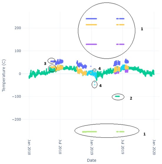
Figure 3. Typical Errors. Colors indicate different sensors, with green indicating NOAA data.

The scikit-learn Python library provided access to the DB index metric. Other metrics for cluster analysis were considered, such as the Dunn Index and the Silhouette Score; however, the available library for the Dunn Index required considerable memory unavailable on any machines used for this work, and the Silhouette Score (also available through scikit-learn) took considerable computational time for the size of the dataset and was disqualified due to time constraints.

This mean difference can be compared against the number of records in each cluster. This and the DB Index can be used for results analysis.

4. Results

Here, we list the results of the various clustering algorithms, their index scores, and the comparison against the NOAA ground-truth data. The sensor data themselves can be seen in Figure 4, Figure 5, Figure 6 and Figure 7. Notice that each node produces different sensor variations per sensor and node, with some sensors and nodes producing more heuristic anomalies than others. Particularly interesting is Figure 6, where no heuristic anomalies are visible, and Figure 7, where very few are present.

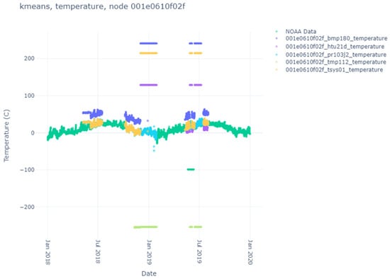
Figure 4. Temperature sensor results for node f02f.

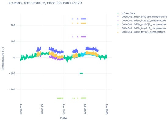
Figure 5. Temperature sensor results for node d620.

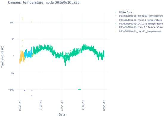
Figure 6. Temperature sensor results for node ba3b.

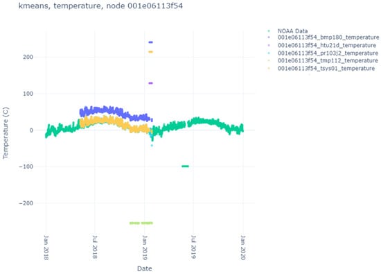
Figure 7. Temperature sensor results for node 3f54.

To properly compare the cluster results of each algorithm to the ground-truth data, we need to calculate the mean difference between relevant sensor readings and the corresponding (by date) NOAA reading. This was performed by heuristically stripping any sensor readings more than 50 degrees Celsius (C) in value from the NOAA reading and any NOAA readings before the first sensor reading, after the last sensor reading, and any missing readings. The difference between each sensor reading and the closest NOAA reading is calculated here. This value is stored, and a mean difference between a given node/sensor combination and the NOAA ground-truth data is calculated. We record ignored sensor readings (readings outside the bounds $\alpha =50$°C). These results can be seen in Table 2.

Table 2. Calculated mean difference between NOAA and sensor reading and heuristically determined anomalies for each sensor.

Node	Sensor	Mean Difference (C)	Heuristic Anomalies
001e0610f02f	bmp180	26.036459540641555	302,412
001e0610f02f	htu21d	9.781522863456273	302,364
001e0610f02f	pr103j2	11.049243296362324	91
001e0610f02f	tmp112	8.374291058850147	325,022
001e0610f02f	tsys01	9.172739785041829	302,405
001e06113d20	bmp180	25.16383727102557	146,584
001e06113d20	htu21d	13.681414767638573	146,585
001e06113d20	pr103j2	7.7000304252925496	0
001e06113d20	tmp112	7.462584734339503	185,959
001e06113d20	tsys01	8.381908452347583	146,672
001e0610ba3b	bmp180	2.506072511582037	0
001e0610ba3b	htu21d	2.267898950715112	57
001e0610ba3b	pr103j2	4.2159915903387635	0
001e0610ba3b	tmp112	2.388445906178256	14
001e0610ba3b	tsys01	2.48385312219104	26
001e06113f54	bmp180	25.6783722548025	30,275
001e06113f54	htu21d	8.900733403493744	30,270
001e06113f54	pr103j2	9.7722823823438	59
001e06113f54	tmp112	7.994874787555069	89,119
001e06113f54	tsys01	9.143470380791154	30,269

Except for one node (ba3b), most sensors operate in individual ranges but generally within a couple of degrees of their sensor counterparts on different nodes and one another (except the bmp180 sensor). This may be attributed to exposure to the environment vs. recording internal heat. What is beneficial is understanding the baseline (mean) difference between what the sensor generally records and the ground-truth data. This can be used to determine how well specific clustering algorithms perform when clustering data into two or more clusters.

We start with the K-Means algorithm. Since the user specifies the number of clusters and we are interested in binary anomaly detection, we set the number of clusters to 2. The values for the K-Means algorithm for each node and sensor can be seen in Table 3. We see immediately that for most nodes and sensors, K-Means successfully determined the same anomalies that were heuristically separated using the value of 50 degrees Celsius (C) (which was arbitrarily chosen before data analysis was conducted). In 8 of the 20 sensors, the number of heuristic anomalies significantly differed from the number of values in the second cluster. For the first case (node f02f, sensor pr103j2), there were 16 previously unknown NaN values for the sensor readings. K-Means detected these and clustered these 16 values in its cluster. For six of the remaining seven instances, the number of heuristic anomalies was so small that K-Means discovered some other feature in the data that was more prevalent. There was only one instance where K-Means failed to properly cluster the heuristic anomalies (node 3f54, sensor htu21d), where the number of heuristic anomalies matched other sensor instances where K-Means successfully matched the counts. The specifics for this change are unknown as the sensor data are not significantly different from another sensor on the same node (tsys01), which is clustered more succinctly.

Table 3. K-Means cluster counts vs. heuristically determined anomalies for each sensor.

Node	Sensor	Clusters	Heuristic Anomalies
001e0610f02f	bmp180	0: 538,608, 1: 302,412	302,412
001e0610f02f	htu21d	0: 538,656, 1: 302,364	302,364
001e0610f02f	pr103j2	1: 869,380, 0: 16	91
001e0610f02f	tmp112	0: 515,424, 1: 325,022	325,022
001e0610f02f	tsys01	0: 538,615, 1: 302,405	302,405
001e06113d20	bmp180	0: 988,385, 1: 146,584	146,584
001e06113d20	htu21d	1: 988,382, 0: 146,585	146,585
001e06113d20	pr103j2	0: 725,652, 1: 410,257	0
001e06113d20	tmp112	0: 911,575, 1: 185,959	185,959
001e06113d20	tsys01	0: 988,298, 1: 146,672	146,672
001e0610ba3b	bmp180	0: 140,726	0
001e0610ba3b	htu21d	0: 139,592	57
001e0610ba3b	pr103j2	1: 275,070, 0: 88,321	0
001e0610ba3b	tmp112	0: 140,951	14
001e0610ba3b	tsys01	0: 131,548	26
001e06113f54	bmp180	0: 876,676, 1: 30,274	30,275
001e06113f54	htu21d	0: 517,333, 1: 389,617	30,270
001e06113f54	pr103j2	0: 551,586, 1: 355,364	59
001e06113f54	tmp112	0: 817,833, 1: 89,119	89,119
001e06113f54	tsys01	0: 876,682, 1: 30,269	30,269

For these next two clustering algorithms, the values of their hyper-parameters can significantly affect the number of clusters created (clusters are created dynamically and not chosen by the user). Due to execution issues and memory overflows due to internal issues with the cuML library and H-DBSCAN running on this subset of data, we selected lower values for the hyper-parameters for H-DBSCAN. To make the comparison fairer, we also selected similar values for the hyper-parameters for DBSCAN. As a result, in some instances, the amount of clusters created was significant. We report the number of clusters generated as well as the largest two clusters (if two or more clusters were generated), as well as any cluster that matches the number of points in the heuristic anomaly column, as well as cluster −1 (if it exists), which represents “noise” in the data as calculated by the algorithms. Table 4 and Table 5 show the results.

Table 4. DBSCAN cluster counts vs. heuristically determined anomalies for each sensor.

Sensor	Notable Clusters	Cluster Count	Heuristic Anomalies
001e0610f02f
bmp180	0: 538,566, 3: 302,412, −1: 23	6	302,412
htu21d	3954: 302,364, 178: 989, −1: 166	3956	302,364
pr103j2	13: 741,737, −1: 98,564	17	91
tmp112	0: 514,774, 2: 325,022, −1: 10	4	325,022
tsys01	1: 532,990, 2: 302,405, −1: 4817	4	302,405
001e06113d20
bmp180	4: 623,832, 3: 364,467, 6: 146,584, −1: 7	8	146,584
htu21d	16: 361,405, 32: 146,585, −1: 16	788	146,585
pr103j2	194: 8314, 191: 8271, −1: 1	408	0
tmp112	7: 152,812, 9: 10,178, −1: 5	633	185,959
tsys01	2: 988,273, 0: 146,672, −1: 5	4	146,672
001e0610ba3b
bmp180	−1: 140,726	1	0
htu21d	−1: 139,592	1	57
pr103j2	0: 363,391	1	0
tmp112	−1: 140,951	1	14
tsys01	−1: 131,548	1	26
001e06113f54
bmp180	0: 876,475, 5: 30,274, −1: 22	13	30,275
htu21d	4076: 30,270, 502: 618, −1: 393	4079	30,270
pr103j2	0: 906,874, −1: 38	5	59
tmp112	721: 30,270, 173: 3537, −1: 23	732	89,119
tsys01	49,675: 30,269, −1: 173,060	49,681	30,269

Table 5. H-DBSCAN cluster counts vs. heuristically determined anomalies for each sensor.

Sensor	Notable Clusters	Cluster Count	Heuristic Anomalies
001e0610f02f
bmp180	2: 319,133, 4: 302,412, −1: 8	6	302,412
htu21d	4: 312,895, 16: 302,364, −1: 8	201	302,364
pr103j2	13: 741,737, −1: 98,564	17	91
tmp112	0: 514,774, 2: 325,022, −1: 10	4	325,022
tsys01	not clustered
001e06113d20
bmp180	4: 623,832, 3: 364,467, 6: 146,584, −1: 7	8	146,584
htu21d	16: 361,405, 32: 146,585, −1: 16	788	146,585
pr103j2	194: 8314, 191: 8271, −1: 1	408	0
tmp112	7: 152,812, 9: 10,178, −1: 5	633	185,959
tsys01	not clustered
001e0610ba3b
bmp180	1: 140,282, 0: 444	2	0
htu21d	−1: 139,592	1	57
pr103j2	57: 3306, 73: 3296, −1: 3	522	0
tmp112	−1: 140,951	1	14
tsys01	not clustered
001e06113f54
bmp180	1: 503,497, 2: 373,091, −1: 6	6	30,275
htu21d	25: 212,746, 26: 199,184, 32: 30,270, −1: 21	287	30,270
pr103j2	484: 7897, 482: 7645, 230: 59, −1: 18	557	59
tmp112	7: 41,991, 9: 13,826, −1: 3	622	89,119
tsys01	not clustered

Interestingly, despite the algorithm chosen, node ba3b routinely clusters with one cluster (often confusing both DBSCAN variants into believing all the data are noise). This is interesting, considering that the small bounds for the hyper-parameters for DBSCAN and H-DBSCAN tend to produce many clusters. As mentioned, H-DBSCAN failed to cluster the tsys01 sensor due to library execution issues; therefore, that information is missing.

Overall, all three algorithms perform well in clustering together the heuristically determined anomalies, with K-Means successfully clustering heuristic anomalies separately 11/17 times (64.71% success), DBSCAN having 10 matching or near-matching heuristic anomaly counts and 7 misses (58.82% success), and H-DBSCAN having 7 matching or near-matching heuristic anomaly counts and 6 misses (53.85% success). Most of the misses for each algorithm (five for K-Means and DBSCAN, and four for H-DBSCAN) occurred when very few heuristic anomalies were present in the data. Given that DBSCAN and H-DBSCAN provide a method to treat small numbers of points as noise, it is not surprising that the algorithms do not properly cluster the heuristic anomalies separately in these cases. By definition of being restricted to only two clusters, K-Means would also find it difficult to cluster such a small number of points in a separate cluster. Again, we specify that no algorithm had access to the ground-truth data or the heuristic labels; all analysis was performed after the runs were complete.

In addition to the analysis against the ground-truth data, we calculated the Davies–Bouldin (DB) score for each node and sensor against each clustering algorithm. In addition, any instance where only one cluster was present has no score since the DB score requires at least two clusters to compare against. The results are seen in Table 6, Table 7 and Table 8.

Table 6. The Davies–Bouldin scores for each node–sensor combination, K-Means algorithm.

Node	Sensor	DB Score
001e0610f02f	bmp180	0.038824672921208406
001e0610f02f	htu21d	0.07690979909983497
001e0610f02f	pr103j2	na
001e0610f02f	tmp112	0.02882118033585473
001e0610f02f	tsys01	0.04384870955257482
001e06113d20	bmp180	0.036814840183613945
001e06113d20	htu21d	0.09983222742572292
001e06113d20	pr103j2	0.4865105225567226
001e06113d20	tmp112	0.029372036351903098
001e06113d20	tsys01	0.042269436817583314
001e0610ba3b	bmp180	na
001e0610ba3b	htu21d	na
001e0610ba3b	pr103j2	0.5345483627490976
001e0610ba3b	tmp112	na
001e0610ba3b	tsys01	na
001e06113f54	bmp180	0.041739643131029645
001e06113f54	htu21d	0.8394572503561166
001e06113f54	pr103j2	0.428926620784116
001e06113f54	tmp112	0.03241690084035104
001e06113f54	tsys01	0.04727127733130374

Table 7. The Davies–Bouldin Scores for each node–sensor combination, DBSCAN algorithm.

Node	Sensor	DB Score
001e0610f02f	bmp180	0.4718700086311703
001e0610f02f	htu21d	5.876686360715116
001e0610f02f	pr103j2	17.36570049090865
001e0610f02f	tmp112	0.4729803974388458
001e0610f02f	tsys01	0.7183360242412649
001e06113d20	bmp180	0.7462073297124467
001e06113d20	htu21d	0.5838881087020173
001e06113d20	pr103j2	0.013257589483531482
001e06113d20	tmp112	0.36487164730951704
001e06113d20	tsys01	0.370089169290952
001e0610ba3b	bmp180	na
001e0610ba3b	htu21d	na
001e0610ba3b	pr103j2	na
001e0610ba3b	tmp112	na
001e0610ba3b	tsys01	na
001e06113f54	bmp180	0.9469419977288394
001e06113f54	htu21d	11.078222823066527
001e06113f54	pr103j2	1.7596756189000833
001e06113f54	Sensor tmp112	1.8624986844262612
001e06113f54	Sensor tsys01	6.097546251475771

Table 8. The Davies–Bouldin scores for each node–sensor combination, H-DBSCAN algorithm.

Node	Sensor	DB Score
001e0610f02f	bmp180	0.5211068325684747
001e0610f02f	htu21d	0.5322988964134147
001e0610f02f	pr103j2	17.36570049090865
001e0610f02f	tmp112	0.4729803974388458
001e0610f02f	tsys01	not clustered
001e06113d20	bmp180	0.7462073297124467
001e06113d20	htu21d	0.5838881087020173
001e06113d20	pr103j2	0.013257589483531482
001e06113d20	tmp112	0.36487164730951704
001e06113d20	tsys01	not clustered
001e0610ba3b	bmp180	0.9228684923154065
001e0610ba3b	htu21d	na
001e0610ba3b	pr103j2	0.01511222997279345
001e0610ba3b	tmp112	na
001e0610ba3b	tsys01	not clustered
001e06113f54	bmp180	0.9694545711960667
001e06113f54	htu21d	1.56414130504102
001e06113f54	pr103j2	17.82433574172976
001e06113f54	tmp112	0.5977439467700165
001e06113f54	tsys01	not clustered

The DB Scores are better (the clusters are more valid) the closer to 0 the value gets. The K-Means algorithm has the best scores of all three algorithms, with all scores below 1 and most scores below 0.1. This would indicate the clusters chosen were dense and separable. The DB Scores for DBSCAN were generally much higher, with all but 1 score above 0.1 and 9 of 15 reported scores above 1. Some cases (node f02f, sensor pr103j2, node 3f54, and sensor htu21d) had very high DB score values. This indicates the clusters were not that separable. This is likely due to the lack of dimensionality in the dataset. With this metric, H-DBSCAN fared better than DBSCAN, having two scores below 0.1 and only three of fourteen reported scores above 1. H-DBSCAN also had two scores (node f02f, sensor pr103j2, node 3f54, sensor pr103j2) with very high DB score values. This would indicate better separability than DBSCAN but worse than K-Means.

The takeaway from this analysis is that, with only a small subset of the available data present in the Chicago AoT, ignoring multi-dimensional node level, spatial, and temporal contexts, these clustering algorithms were still capable of automatically clustering anomalies selected by a heuristic without the need to develop a rule to do so. This result shows the promise of utilizing the Chicago AoT for more complex anomaly detection.

5. Conclusions

In this work, we discuss the Chicago Array of Things (AoT), its usefulness for anomaly detection, and the capability of three well-known clustering algorithms (K-Means, DBSCAN, and H-DBSCAN) in sensor-level clustering to label the dataset.

We have shown that at the sensor level, these algorithms are capable of automatically (without user input) separating the data in cases where there are large amounts of visually discernible anomalies; that is, anomalies that, when seen by a user, would be flagged as such, without the need to develop specific rules to do so. The drawback of this approach is that, by focusing on the sensor level, these algorithms lack the context of multi-dimensional data (for instance, treating all sensors on a node as a single multi-dimensional data point) and spatial and temporal influences.

At the sensor level, when taking into account binary classification (anomalous/non-anomalous), the K-Means algorithm, though simpler, is better suited for the task of determining these heuristic anomalies than the more complex DBSCAN and HDBSCAN algorithms. However, it has drawbacks (such as clustering NaN values as its cluster or clustering based on other factors when very few heuristic anomalies exist in the data).

The results of this work show the potential for the Chicago AoT to be used as a tool for training anomaly detection models by implementing more robust clustering mechanisms with the data.

References

- Chen, K.; Hu, J.; Zhang, Y.; Yu, Z.; Jinliang, H. Fault Location in Power Distribution Systems via Deep Graph Convolutional Networks. IEEE J. Sel. Areas Commun. 2019, 38, 119–131. [Google Scholar] [CrossRef]
- Chen, Z.; Xu, J.; Peng, T.; Yang, C. Graph Convolutional Network-Based Method for Fault Diagnosis Using a Hybrid of Measurement and Prior Knowledge. IEEE Trans. Cybern. 2021, 52, 9157–9169. [Google Scholar] [CrossRef] [PubMed]
- Yu, X.; Yang, X.; Tan, Q.; Shan, C.; Lv, Z. An edge computing based anomaly detection method in IoT industrial sustainability. Appl. Soft Comput. 2022, 128, 109486. [Google Scholar] [CrossRef]
- Su, Y.; Zhao, Y.; Niu, C.; Liu, R.; Sun, W.; Pei, D. Robust Anomaly Detection for Multivariate time-series through Stochastic Recurrent Neural Network. In Proceedings of the 25th ACM SIGKDD International Conference on Knowledge Discovery and Data Mining, Anchorage, AK, USA, 4–8 August 2019; pp. 2828–2837. [Google Scholar] [CrossRef]
- Ngo, Q.D.; Nguyen, H.T.; Tran, H.A.; Pham, N.A.; Dang, X.H. Toward an Approach Using Graph-Theoretic for IoT Botnet Detection. In Proceedings of the 2021 2nd International Conference on Computing, Networks and Internet of Things, Beijing, China, 20–22 May 2021. [Google Scholar] [CrossRef]
- Li, C.; Shen, G.; Sun, W. Cross-Architecture Internet-of-Things Malware Detection Based on Graph Neural Network. In Proceedings of the 2021 International Joint Conference on Neural Networks (IJCNN), Shenzhen, China, 18–22 July 2021; pp. 1–7. [Google Scholar] [CrossRef]
- Beckman, P.; Sankaran, R.; Catlett, C.; Ferrier, N.; Jacob, R.; Papka, M. Waggle: An open sensor platform for edge computing. In Proceedings of the 2016 IEEE SENSORS, Orlando, FL, USA, 30 October–3 November 2016; pp. 1–3. [Google Scholar] [CrossRef]
- Catlett, C.E.; Beckman, P.H.; Sankaran, R.; Galvin, K.K. Array of Things: A Scientific Research Instrument in the Public Way: Platform Design and Early Lessons Learned. In Proceedings of the 2nd International Workshop on Science of Smart City Operations and Platforms Engineering, Pittsburgh, PA, USA, 18–21 April 2017; pp. 26–33. [Google Scholar] [CrossRef]
- Catlett, C.; Beckman, P.; Ferrier, N.; Nusbaum, H.; Papka, M.E.; Berman, M.G.; Sankaran, R. Measuring Cities with Software-Defined Sensors. J. Soc. Comput. 2020, 1, 14–27. [Google Scholar] [CrossRef]
- Daepp, M.I.G.; Cabral, A.; Ranganathan, V.; Iyer, V.; Counts, S.; Johns, P.; Roseway, A.; Catlett, C.; Jancke, G.; Gehring, D.; et al. Eclipse: An End-to-End Platform for Low-Cost, Hyperlocal Environmental Sensing in Cities. In Proceedings of the 2022 21st ACM/IEEE International Conference on Information Processing in Sensor Networks (IPSN), Milano, Italy, 4–6 May 2022; pp. 28–40. [Google Scholar] [CrossRef]
- Catlett, C.; Beckman, P.; Ferrier, N.; Papka, M.E.; Sankaran, R.; Solin, J.; Taylor, V.; Pancoast, D.; Reed, D. Hands-On Computer Science: The Array of Things Experimental Urban Instrument. Comput. Sci. Eng. 2022, 24, 57–63. [Google Scholar] [CrossRef]
- Chen, L.J.; Ho, Y.H.; Hsieh, H.H.; Huang, S.T.; Lee, H.C.; Mahajan, S. ADF: An Anomaly Detection Framework for Large-Scale PM2.5 Sensing Systems. IEEE Internet Things J. 2018, 5, 559–570. [Google Scholar] [CrossRef]
- English, N.; Zhao, C.; Brown, K.L.; Catlett, C.; Cagney, K. Making Sense of Sensor Data: How Local Environmental Conditions Add Value to Social Science Research. Soc. Sci. Comput. Rev. 2022, 40, 179–194. [Google Scholar] [CrossRef] [PubMed]
- Hu, Y.; Wang, Y.; Jiao, C.; Sankaran, R.; Catlett, C.; Work, D. Automatic data cleaning via tensor factorization for large urban environmental sensor networks. In Proceedings of the NeurIPS 2019 Workshop on Tackling Climate Change with Machine Learning, Vancouver, BC, Canada, 14 December 2019. [Google Scholar]
- Oceanographic, N.; National Oceanic and Atmospheric Administration. Climate Data Online: Dataset Discovery. Available online: https://www.ncdc.noaa.gov/cdo-web/datasets (accessed on 22 September 2013).
- Wu, Y.; Dai, H.N.; Tang, H. Graph Neural Networks for Anomaly Detection in Industrial Internet of Things. IEEE Internet Things J. 2022, 9, 9214–9231. [Google Scholar] [CrossRef]
- Šabić, E.; Keeley, D.; Henderson, B.; Nannemann, S. Healthcare and anomaly detection: Using machine learning to predict anomalies in heart rate data. AI Soc. 2021, 36, 149–158. [Google Scholar] [CrossRef]
- Reddy, T.; RM, S.P.; Parimala, M.; Chowdhary, C.L.; Hakak, S.; Khan, W.Z. A deep neural networks based model for uninterrupted marine environment monitoring. Comput. Commun. 2020, 157, 64–75. [Google Scholar] [CrossRef]
- Pang, G.; Shen, C.; van den Hengel, A. Deep Anomaly Detection with Deviation Networks. In Proceedings of the 25th ACM SIGKDD International Conference on Knowledge Discovery and Data Mining, Anchorage, AK, USA, 4–8 August 2019; pp. 353–362. [Google Scholar] [CrossRef]
- Zheng, L.; Li, Z.; Li, J.; Li, Z.; Gao, J. AddGraph: Anomaly Detection in Dynamic Graph Using Attention-based Temporal GCN. In Proceedings of the Twenty-Eighth International Joint Conference on Artificial Intelligence, Macao, China, 10–16 August 2019. [Google Scholar]
- Guttman, A. R-Trees: A Dynamic Index Structure for Spatial Searching. SIGMOD Rec. 1984, 14, 47–57. [Google Scholar] [CrossRef]
- APERIO. Identifying and Managing Risks of Sensor Drift. Available online: https://aperio.ai/sensor-drift/ (accessed on 26 September 2023).
- DeMedeiros, K.; Hendawi, A.; Alvarez, M. A Survey of AI-Based Anomaly Detection in IoT and Sensor Networks. Sensors 2023, 23, 1352. [Google Scholar] [CrossRef] [PubMed]
- Asanka, P.D.; Rajapakshe, C.; Takahashi, M. Identifying Unusual Human Movements Using Multi-Agent and Time-Series Outlier Detection Techniques. In Proceedings of the 2023 3rd International Conference on Advanced Research in Computing (ICARC), Belihuloya, Sri Lanka, 23–24 February 2023; pp. 1–6. [Google Scholar] [CrossRef]
- Lee, C.; Lee, J.; Lee, B.; Park, J.; Park, J.; Kim, Y.; Park, J. Development of Outlier Detection Algorithms for Sensors with Time-Varying Characteristics. In Proceedings of the 2023 34th Annual SEMI Advanced Semiconductor Manufacturing Conference (ASMC), Saratoga Springs, NY, USA, 1–4 May 2023; pp. 1–4. [Google Scholar] [CrossRef]
- Lyu, F.; Wang, S.; Han, S.Y.; Catlett, C.; Wang, S. An integrated cyberGIS and machine learning framework for fine-scale prediction of Urban Heat Island using satellite remote sensing and urban sensor network data. Urban Infomatics 2022, 1, 6. [Google Scholar] [CrossRef] [PubMed]
- Mera-Gaona, M.; Neumann, U.; Vargas-Canas, R.; López, D.M. Evaluating the impact of multivariate imputation by MICE in feature selection. PLoS ONE 2021, 16, e0254720. [Google Scholar] [CrossRef]
- Zhang, Z. Missing data imputation: Focusing on single imputation. Ann. Transl. Med. 2016, 4, 9. [Google Scholar] [PubMed]
- MacQueen, J. Some methods for classification and analysis of multivariate observations. In Proceedings of the Fifth Berkeley Symposium on Mathematical Statistics and Probability, Oakland, CA, USA, 1 January 1967. [Google Scholar]
- Lloyd, S. Least squares quantization in PCM. IEEE Trans. Inf. Theory 1982, 28, 129–137. [Google Scholar] [CrossRef]
- Louhichi, S.; Gzara, M.; Ben Abdallah, H. A density based algorithm for discovering clusters with varied density. In Proceedings of the 2014 World Congress on Computer Applications and Information Systems (WCCAIS), Hammamet, Tunisia, 17–19 January 2014; pp. 1–6. [Google Scholar] [CrossRef]
- Campello, R.J.G.B.; Moulavi, D.; Sander, J. Density-Based Clustering Based on Hierarchical Density Estimates. In Springer Advances in Knowledge Discovery and Data Mining; Pei, J., Tseng, V.S., Cao, L., Motoda, H., Xu, G., Eds.; Springer: Berlin/Heidelberg, Germany, 2013; pp. 160–172. [Google Scholar]
- Stewart, G.; Al-Khassaweneh, M. An Implementation of the HDBSCAN* Clustering Algorithm. Appl. Sci. 2022, 12, 2405. [Google Scholar] [CrossRef]
- Davies, D.L.; Bouldin, D.W. A Cluster Separation Measure. IEEE Trans. Pattern Anal. Mach. Intell. 1979, PAMI-1, 224–227. [Google Scholar] [CrossRef]
- Viegas, J. Small Module with Cluster Validity Indices (CVI). Available online: https://github.com/jqmviegas/jqm_cvi (accessed on 3 October 2023).
- for Geeks, G. Dunn Index and DB Index—Cluster Validity Indices. Available online: https://www.geeksforgeeks.org/dunn-index-and-db-index-cluster-validity-indices-set-1/# (accessed on 3 October 2023).
- Laboratory, A.N. Waggle Sensors. Available online: https://github.com/waggle-sensor/sensors/tree/master/sensors/datasheets (accessed on 6 December 2023).
- numFOCUS. Pandas. Available online: https://pandas.pydata.org/ (accessed on 22 September 2023).
- Foundation, A.S. Apache Spark. Available online: https://spark.apache.org/ (accessed on 22 September 2023).
- Scikit-Learn Developers. Scikit-Learn. Available online: https://scikit-learn.org/stable/index.html (accessed on 22 September 2023).
- NVIDIA. RAPIDS GPU Accelerated Data Science. Available online: https://rapids.ai/ (accessed on 22 September 2023).
- National Park Service. Death Valley National Park. Available online: https://www.nps.gov/deva/learn/nature/weather-and-climate.htm (accessed on 30 November 2023).
Disclaimer/Publisher’s Note: The statements, opinions and data contained in all publications are solely those of the individual author(s) and contributor(s) and not of MDPI and/or the editor(s). MDPI and/or the editor(s) disclaim responsibility for any injury to people or property resulting from any ideas, methods, instructions or products referred to in the content. |
© 2024 by the authors. Licensee MDPI, Basel, Switzerland. This article is an open access article distributed under the terms and conditions of the Creative Commons Attribution (CC BY) license (https://creativecommons.org/licenses/by/4.0/).