1. Introduction
Fifth-generation (5G) networks allow for high-speed data transmission and a wide range of services for numerous users, ensuring high quality of service (QoS) [
1,
2,
3]. The three main scenarios considered are enhanced mobile broadband (eMBB), massive machine-type communication (mMTC), and ultra-reliable low-latency communication (URLLC) [
4]. Beyond 2030, the sixth-generation (6G) network is anticipated to address the need for global coverage; improved spectral, energy, economic efficiency; and enhanced security. To meet these requirements, novel technologies and systems need to be supported on the radio interface and core network, incorporating multiple access, channel-coding schemes, multi-antenna technology, cell-less architecture, cloud/fog computing, and network slicing [
5,
6].
Network slicing is a comprehensive concept that encompasses both network and cloud slices, including radio access, transport, and edge computing network [
7,
8]. It allows for the deployment of multiple logical, autonomous, and independent network resources, as well as network and service functions, on a single infrastructure platform. Through this management mechanism, resource providers can allocate logically isolated network slices to users, each designed and optimized for specific requirements (e.g., one for cellular communication, another for the Internet of Things (IoT)).
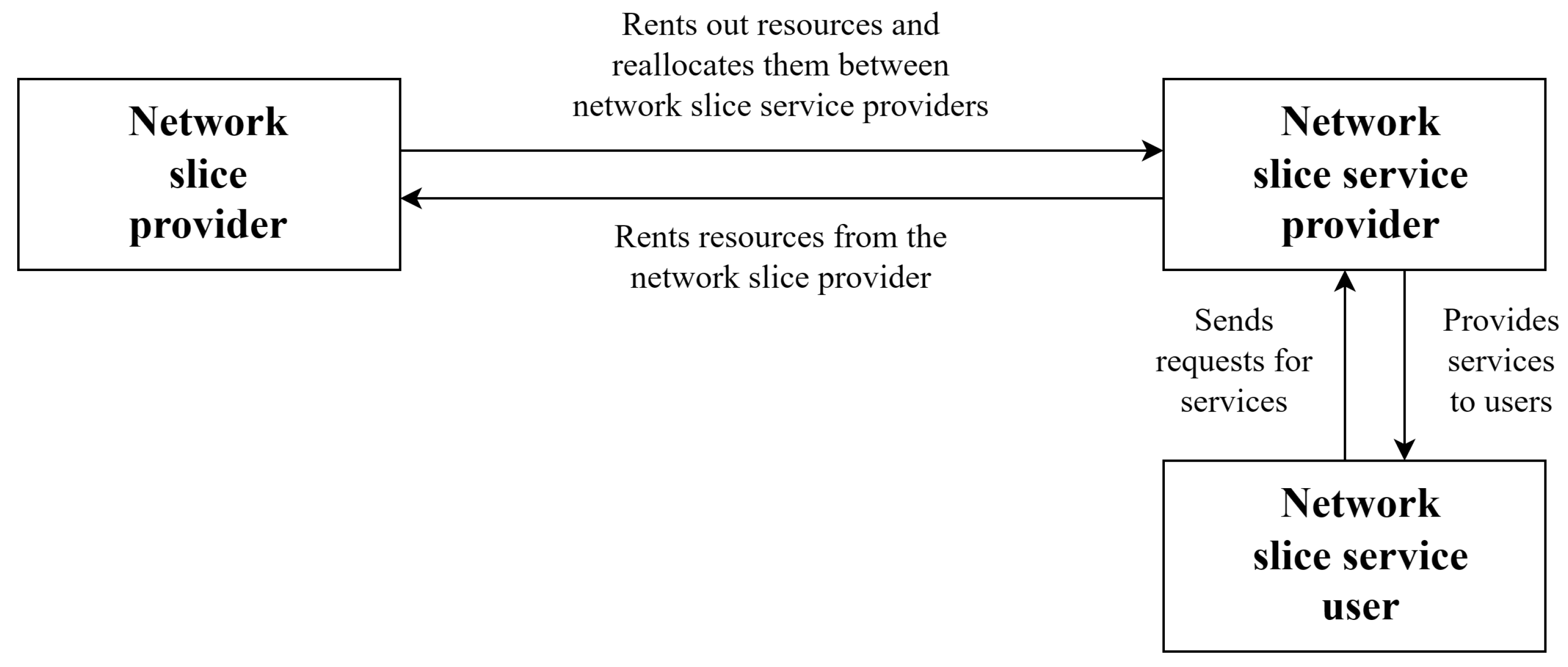
Network slicing assumes three business roles: (i) network slice provider (network operator), which is the resource owner and provides the network slice instance; (ii) network slice service provider (communication service provider), which is responsible for providing services to its users; (iii) network slice service user (communication service customer), which uses the provided services [
9]. The interactions between two business roles are handled through service-level agreements (SLAs), as shown in
Figure 1.
The question of organizing resource reallocation in 5G network slicing has been addressed in recent research papers. For a review of these works, please refer to
Section 2. This paper focuses on modeling and analyzing resource capacity planning and reallocation for network slicing between two providers transmitting elastic traffic, such as during web browsing. The controller sends signals to determine the need for resource reallocation and to plan new resource capacity. A Markov decision process (MDP) is utilized in a controllable queuing system to find the optimal resource capacity for each provider. The reward function incorporates three network slicing principles, including maximum matching for equal resource partitioning, maximum share of signals resulting in resource reallocation, and maximum resource utilization. An iterative algorithm is used to find the optimal resource reallocation policy, and the results are numerically illustrated for two services: web browsing and bulk data transfer.
The main contributions of our study are as follows:
Innovative mathematical framework. We propose a mathematical framework based on queuing theory and MDP. This framework incorporates three weighted principles: maximum matching for equal resource partitioning, maximum share of signals for resource reallocation, and maximum resource utilization. This multi-principle approach is novel in the context of 5G network slicing, providing a comprehensive and flexible foundation for resource capacity planning.
Efficient algorithm development. An algorithm was developed to efficiently compute the optimal resource capacity planning policy. This algorithm leverages R. Howard’s iteration, starting with maximum resource utilization as the initial point. The efficiency and effectiveness of this algorithm contribute to the novelty of our work, ensuring practical applicability in the dynamic environment of 5G network slicing.
Numerical analysis and insights. Our study includes a detailed numerical analysis that not only illustrates the optimal policy but also provides key metrics related to resource utilization and the probability of a signal triggering resource reallocation. The numerical results demonstrate rapid convergence within three iterations, highlighting the efficiency of our proposed approach. This insight is a unique contribution to the field, showcasing the advancements of our balanced three-principle approach to resource capacity planning in 5G network slicing.
The rest of the paper is organized as follows:
Section 2 provides an overview of related work in the field of network slicing.
Section 3 details the system model, while
Section 4 presents the queuing model for the baseline algorithm for resource reallocation.
Section 5 constructs a controllable queuing model to solve the problem of optimal resource reallocation. Illustrative numerical results are presented in
Section 6, and conclusions are drawn in the final section.
2. Fifth-Generation Network Slicing and Related Work
In this section, we review some selected papers on network slice service planning and resource capacity planning.
2.1. Network Slice Service Planning
The most frequently cited use case for network slicing is presented in [
10] and is based on three 5G scenarios: eMBB for high data rates, high user density, and high user mobility; mMTC for a small number of latency-insensitive data; and URLLC for strict requirements for throughput, latency, and reliability. For example, in a self-driving car, a user could simultaneously access different network slices. A self-driving car is connected to the network through vehicle-to-everything (V2X) communication. The user sitting in the car initiates a service for HD video streaming using the system available in the car. V2X communication requires low latency but not necessarily a high data rate, while HD video streaming requires a high data rate but is latency-tolerant. Thus, the V2X communication service and HD video streaming service connect to different network slices, such as a URLLC slice and an eMBB slice.
Network slices could be organized for mobile virtual network operators (MVNOs). This is the use case where a mobile network operator (MNO), as a network slice provider, leases its radio resources to MVNOs as network slice service providers who do not own wireless network infrastructure. MNO and MVNOs conclude SLAs that define the boundaries of slices depending on the requirements of services. Another often used case is organizing network slices for different traffic types, for example, for guaranteed bit rate (GBR) traffic with a minimum-bit-rate guarantee and for non-GBR traffic without such guarantees. Traffic could be viewed as streaming traffic when a service generated it and is characterized by its duration, while elastic traffic services are characterized by the size of the transmitted data.
Table 1 provides references with the above-mentioned examples of network slice service planning mechanisms.
2.2. Resource Capacity Planning
Resource capacity planning can be achieved through either static resource partitioning or dynamic resource reallocation. Static resource partitioning involves allocating resources to network slices that do not change over time. On the other hand, dynamic resource reallocation involves changing resource allocation among slices over time, as determined by the controller, which periodically checks the need for change. Various mechanisms and criteria are considered during resource capacity planning, including slice priorities, weights, resource utilization, fairness, availability, and isolation (see
Table 1).
Network slice isolation is a crucial factor in resource capacity planning. Although not yet fully formalized in specifications, it is generally understood as minimizing the impact of one slice on the performance of other slices. Isolation is often provided until the number of users exceeds a given threshold. In cases where there is a shortage of resources, users who violate isolation may be interrupted by users from other slices. Slice degradation, defined as a state where one or more active users are not provided with the necessary resources to fulfill bit-rate guarantees, is closely related to isolation.
The efficiency of resource capacity planning depends on the resource reallocation policy among network slices. Mathematical methods commonly used to solve corresponding optimization problems include optimization theory for linear and nonlinear problems, game theory, cooperative game theory (Nash equilibrium), machine learning [
37], MDP, continuous-time Markov chain (CTMC), and queuing theory. A retrial queuing system with an infinite orbit was proposed for analyzing prioritization schemes and resource reservation [
38]. In another study [
39], a resource queuing system with signals, where upon arrival, the signal interrupts a user to try again with a new bit-rate requirement, was analyzed.
2.3. Related Work Employing Markov Decision Process
Efficient resource allocation policies among network slices have a direct impact on resource utilization. Active research efforts are currently focused on the effective management of network resources using the network slicing technique. MDP, a widely utilized mathematical approach to optimization issues, is also employed in our study. The
Table 2 summarizes various recent studies that have applied this method.
2.4. Our Previous Work
This paper focuses on a service generating impatient elastic traffic and is a continuation of our previous research, which analyzed the process of elastic traffic transmission [
48]. We expanded the model to two network slices with dynamic resource reallocation initiated not by the controller but by all events that could influence the need for resource reallocation [
49]. To assess the effectiveness of resource reallocation, we proposed three criteria that are also used in this paper [
50]. This paper proposes a more flexible system that allows for the selection of a new number of allocated resources depending on the network load. To address this issue, we utilized controllable queuing systems [
51,
52,
53].
3. System Model
In this section, we discuss the considered system model, emphasizing the role of the controller in resource reallocation. Then, we describe an algorithm for resource reallocation oriented towards maximum resource utilization. This algorithm serves as a baseline “fixed” algorithm, meaning that it is a function assigning a new resource partitioning to each system state. Additionally, we introduce two other principles that will be taken into account in the model for the construction of a “flexible” algorithm, considering not only resource utilization.
3.1. Preliminary Considerations
Our system model is predicated on a set of simplifying assumptions. We focus on a scenario involving just two network slice service providers, between whom resources are dynamically reallocated. The arrival patterns of both controller signals and user requests are inherently stochastic. Resource reallocation is contingent upon the receipt of a signal from the controller. Within each slice, we posit an egalitarian distribution of resources among all users, irrespective of their remaining service duration, adhering to what is known as the Egalitarian Process Sharing discipline in queueing theory. All system events are assumed to follow an exponential distribution. For our numerical analysis, we chose to examine two distinct services: web browsing and bulk data transfer.
The controller is the pivotal element in our network slicing model, dictating when resource reallocation should occur. The output of the controller’s operation is the allocation of resources to the first slice—knowing that this allows us to deduce the resource allocation for the second slice, given that the total resource pool remains constant. This allocation is part of what we refer to as the control strategy. The controller’s signal rate is a critical factor influencing system performance and resource reallocation; hence, it is incorporated into the reward function discussed in
Section 5.4.
Our system’s self-optimization mechanisms operate by adjusting weights across three key components that collectively enhance system efficiency. This self-optimization entails fine-tuning policy computation based on the reward function’s configuration, thereby directly influencing the selection and nature of the optimal policy. During the optimization process, we determine new resource allocation operations in response to the reward function, ensuring that the optimal policy is shaped by this function. In scenarios where only a baseline algorithm exists, we establish the policy analytically. Policies influenced by the reward function are presented in tabular form. We identify three primary risks: underutilization of resources, non-impactful controller signals, and deviations from QoS allocation. These risks are integrated into the reward function, and by modulating their respective weights, we can prioritize certain risks over others according to their significance within our framework.
3.2. General Assumptions
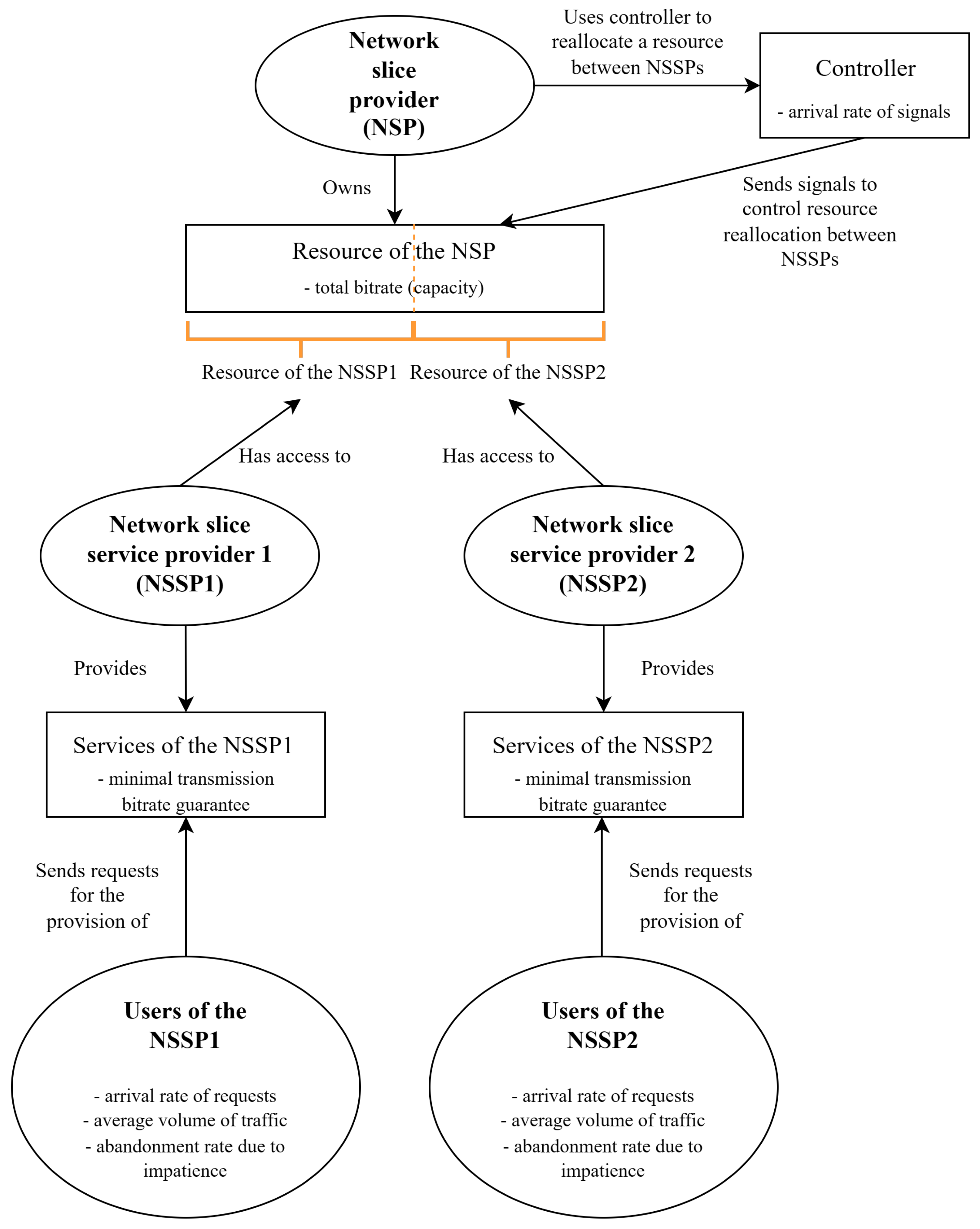
We consider a network slice provider (network operator) with a total capacity (bit rate) of
C bps, which is shared between two network slice service providers (communication service providers), denoted by
. Each service provider has its own network slice service users (communication service customers). The resource reallocation between the service providers is managed by the network slice provider’s controller, which sends signals to determine the need for resource reallocation. The time between signal arrivals follows an exponential distribution with parameter
. The decision-making process is based on three principles: maximum matching for equal resource partitioning, maximum share of signals resulting in resource reallocation, and maximum resource utilization. Each principle is assigned a weight, denoted by
,
, and
, respectively. The motivations behind these weights will be discussed in
Section 3.5. The general scenario is illustrated in
Figure 2.
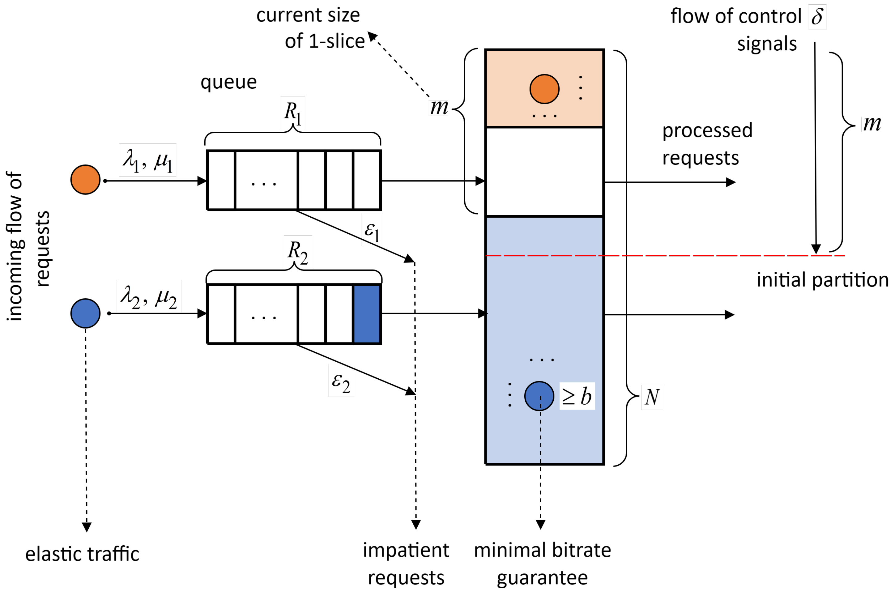
The network slice service provider offers its users a service for transmitting elastic traffic with a minimum-bit-rate guarantee of b. This means that the maximum number of all providers’ users jointly transmitting elastic traffic is equal to . The delay in transmission is acceptable, but the maximum number of users for each provider waiting for delayed elastic traffic transmission is limited to (size of the provider’s buffer). Requests for elastic traffic transmission from users arrive at a rate of according to a Poisson process. The volume of elastic traffic transmitted by each user is exponentially distributed with an average of . Each user is also impatient and spends an exponentially distributed amount of time in their provider’s buffer with a parameter of (abandonment rate).
The system employs the Egalitarian Process Sharing discipline to manage traffic fluctuations. This approach ensures equitable allocation of resources. Resources within each slice are distributed equally, fostering a just and effective use of the system’s capacities. It is crucial to note that requests are received independently. All of the aforementioned parameters are presented in
Figure 3 and listed in
Table 3.
3.3. Resource Reallocation by Controller
The controller plays a crucial role in implementing resource capacity planning by periodically sending signals to assess the need for resource reallocation. The main responsibility of the controller is to determine the most effective method for scheduling resources, guided by three principles: maximum matching for equal resource partitioning, maximum share of signals resulting in resource reallocation, and maximum resource utilization.
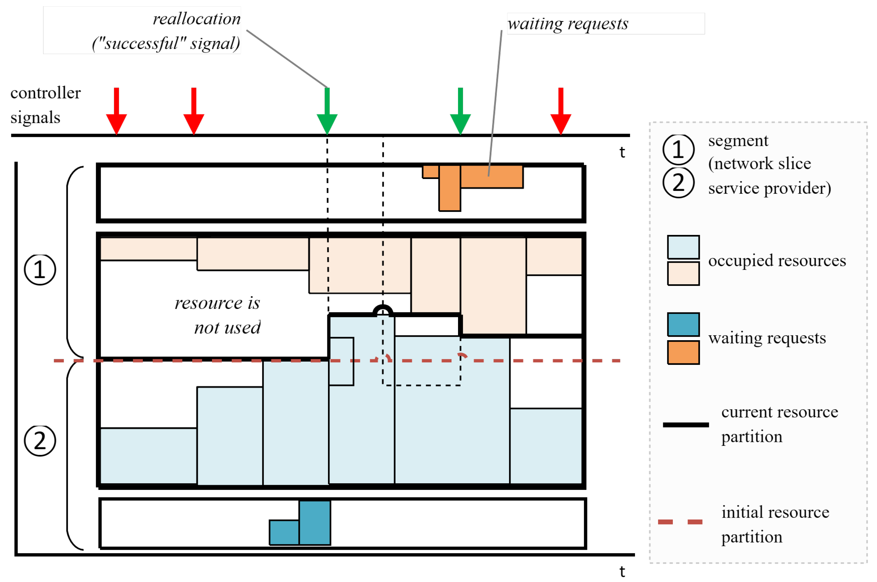
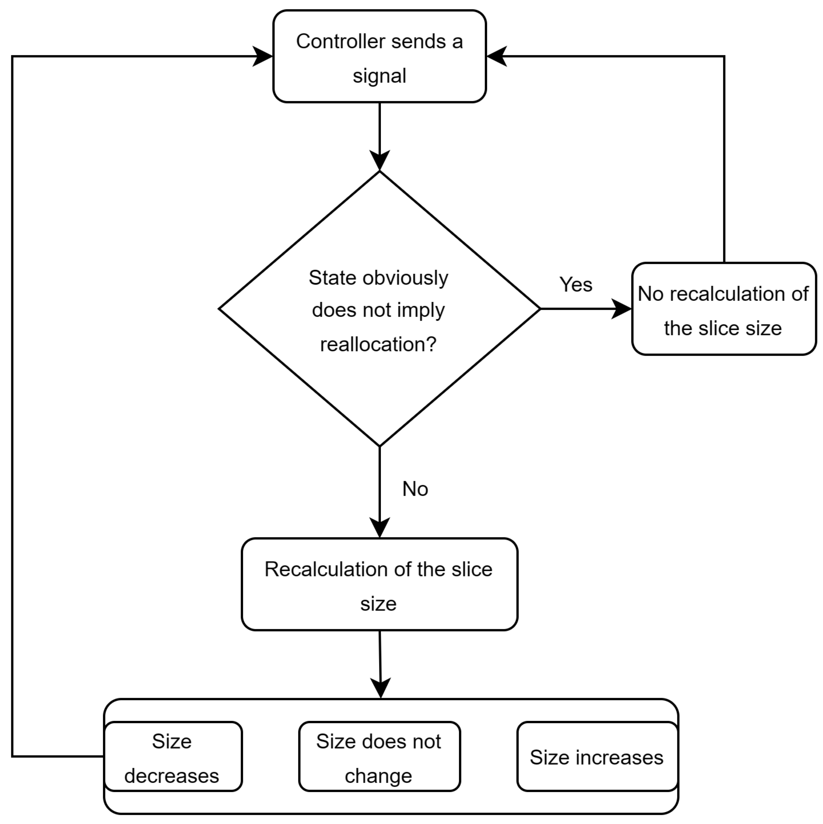
Resource reallocation is triggered when the controller sends a signal and there are unused resources in one slice while there are pending requests from another slice. This type of signal is referred to as “resulting” and leads to resource reallocation. However, if all buffers are empty or all resources are currently in use when a signal is received, no reallocation occurs. Please refer to
Figure 4 for a visual representation. Furthermore, during reallocation, the controller takes into account the average volume of elastic traffic conveyed by
k-users
.
3.4. Baseline Algorithm for Resource Reallocation
Let us present a detailed description of a baseline algorithm for resource reallocation that is designed to maximize resource utilization. Resource reallocation may occur when a signal is received from the controller.
Resource reallocation is triggered under the following conditions:
The resources in the 1-slice are fully occupied, while there are still users waiting for service. However, there are available resources in the 2-slice. In this case, some of the idle resources in the 2-slice are reassigned to the 1-slice.
Similarly, if the resources in the 2-slice are fully occupied and there are users waiting for service, but there are available resources in the 1-slice, some of the idle resources in the 1-slice are reassigned to the 2-slice.
On the other hand, resource reallocation does not take place if any of the following conditions occur:
The system is empty.
Not all resources are occupied (i.e., there are available resources in both the 1-slice and 2-slice).
All resources are occupied, but there are no users waiting for service.
All resources are occupied, and there are users waiting for service from only one slice.
All resources are occupied, and there are users waiting for service from both the 1-slice and 2-slice.
3.5. Three Principles for Resource Reallocation
Note that frequent signals allow for more flexible resource allocation but also increase the load on the system. This poses a problem of how to adjust the rate of controller signals in order to balance compliance with equal resource partition, maximize resource utilization, and increase the number of signals that result in resource reallocation. Additionally, it is important to consider the extent to which the boundaries of resource slices should be adjusted.
The controller manages resource reallocation based on three principles, each with a weight , where :
The first principle takes into account the deviation from equal resource partition, specifically the number of requests that could be served but are waiting due to unequal resource partition. This is significant because the optimal policy should align with the initial partition outlined in the service-level agreement (SLA) between the network slice provider and network slice service providers.
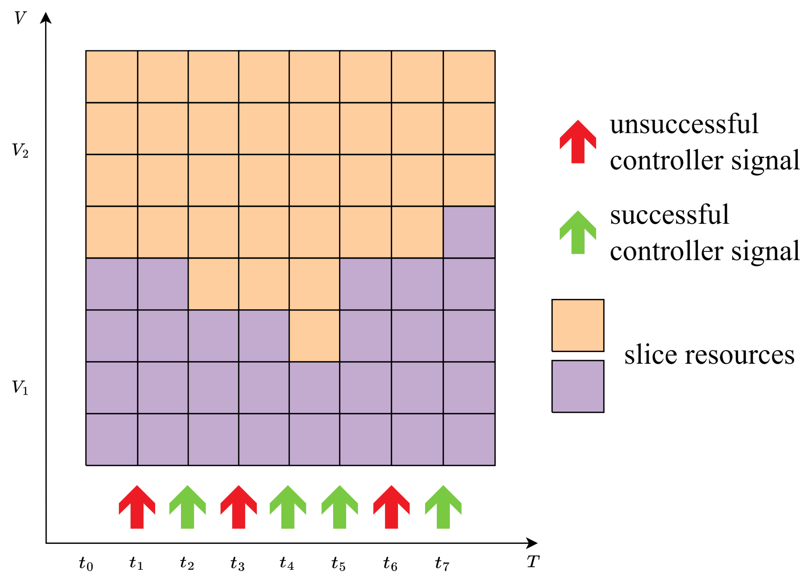
The second principle considers the frequency of cases where resource reallocation does not occur when a signal arrives. It is crucial that signals from the controller result in real resource reallocation. Frequent arrival of “non-resulting” signals is deemed unacceptable, as it incurs unnecessary signaling messages. This aspect is also relevant in radio resource management strategies, as it can affect resource efficiency and utilization. An example is shown in
Figure 5.
The third principle evaluates the number of free resources while users are waiting. In this case, maximizing resource utilization is important. Idle resources, representing the situation where a user is waiting for a slice that is currently occupied and another slice is available to serve the user’s request, are undesirable.
4. Queuing Model for Baseline Algorithm
In this section, we will introduce a queuing model for the baseline algorithm discussed previously.
4.1. Continuous-Time Markov Chain
Let us describe the system model using a corresponding queuing system, as shown in
Figure 6. Continuous-time Markov chain (CTMC)
has states
, where
m represents the maximum number of 1-users jointly transmitting elastic traffic (size of 1-slice), and
represents the number of k-users transmitting elastic traffic and waiting in
k-buffer. The state space is presented as follows:
4.2. State-Space Decomposition
Let us decompose system state space (
1) into smaller subsets for better analysis. Note that
represents the maximum number of 2-users that can jointly transmit elastic traffic. The partitioning of set
into subsets is based on two factors: the possibility of resource reallocation and the ratio of users transmitting traffic to those waiting in buffers. We define
as the states where resource reallocation occurs upon receiving a signal and
as the states in which it does not occur. Hence,
can be represented as a union of these two disjoint subsets:
Moreover, we know that
m is the parameter used in the reallocation management policy to determine the size of the 1-slice. Thus, we can express
as a union of subsets corresponding to different values of
m:
Furthermore, we can divide subset
into two more subsets:
and
, where
represents states in which the size of the 1-slice is increased upon receiving a signal and
represents states in which the size of the 2-slice is increased upon receiving a signal.
Finally, in the case where there are enough free resources to serve waiting users, the slices are increased either by the number of waiting users or by all free resources. Thus, the subset of
can be represented as the following union:
4.3. Transition Rates between CTMC States
Table 4 displays the transition rates from current state
to
. Only transition rates pertaining to users are included in this table. When a signal arrives at rate
, the system transitions to state
, where
5. Controllable Queuing Model
In this section, we discuss a more complex policy that not only maximizes resource utilization but also maximizes the share of signals resulting in resource reallocation and maximum matching for equal resource partitioning.
5.1. Continuous-Time Markov Decision Process
To address the issue of optimal resource reallocation, it is crucial to select the best course of action for determining the volume of resources to be reallocated based on the current state of the system. This problem can be defined as a continuous-time MDP. The MDP model is represented by a four tuple :
Set
of states
, defined by Formula (
1);
Set of actions a available from state ;
Matrix of transition rates under action a;
Reward received while in state .
5.2. Action Space for Resource Reallocation
The control policy for the two-slice model dictates the necessary actions to adjust the size of the 1-slice in response to a signal from the controller. This adjustment is only applicable to states within subset
, where resource reallocation is required. The action space can be divided into four cases, based on the ratio of users transmitting traffic and waiting in buffers for each slice. If both buffers are either free or occupied, no reallocation occurs upon receiving a signal. However, if one buffer is free while the other is occupied, resource reallocation can be initiated. Therefore, the set of action space (
) can be defined as follows:
5.3. Transition Rates between MDP States
Transition rates are determined by
Table 4 and
Table 5 with an intensity of
. Thus, rate
for action
a in state
leading to state
is calculated using the following formula:
5.4. Reward Function to Consider Three Principles
In accordance with the previously described principles of reallocation, the reward function received per unit time during the stay in state
is defined by the following formula:
Let us describe each component in detail.
The principle of maximum matching for equal resource partitioning is determined by the number of users waiting in the buffer due to unequal resource reallocation and is defined as
The principle of maximum share of signals resulting in resource reallocation is determined by the probability of non-reallocation after a signal is received and is given by the following formula:
The principle of maximum resource utilization is determined by the number of users waiting in the buffer due to idle resources, expressed as
To elucidate this principle with greater clarity, consider the initial equation within system . This equation signifies that the 1-slice possesses a surplus of users in its 1-buffer (where ), and concurrently, the 2-slice has available resources (). Additionally, the combined total , indicating that the quantity of users awaiting the 1-slice surpasses the idle resources of the 2-slice, resulting in an inability to serve all waiting users. Consequently, we allocate the utmost number of idle resources from the 2-slice to attend to the greatest possible number of waiting users. In this scenario, the resource volume equates to the entirety of idle resources from the 2-slice, expressed as (where represents the count of occupied resources in the 2-slice).
Moving on to the second equation, implies that there are users awaiting service in the 1-buffer for the 1-slice (), while there are unutilized resources in the 2-slice (), and . This situation indicates that the number of users waiting for the 1-slice is either less than or equal to the idle resources available in the 2-slice, ensuring all waiting users can be accommodated. Thus, we engage the precise number of necessary idle resources from the 2-slice, which, in this case, corresponds to the count of waiting users from the 1-slice, or . The third and fourth equations present analogous circumstances, yet they involve an augmentation in the volume of resources for the 2-slice.
Furthermore, the network slice provider has the ability to determine which of these principles is the most important and can adjust their relative importance. Each principle is assigned a weight to indicate its significance. The reward function is expressed with a negative sign to represent a “penalty” for incorrect resource reallocation.
5.5. Policy Iteration by R. Howard
Let us define the average reward as
where
is the stationary probability distribution.
The system of equations for the average reward (
) and estimates
,
, for the iterative solution method is given as
The objective function for improving the control policy is calculated using the formula
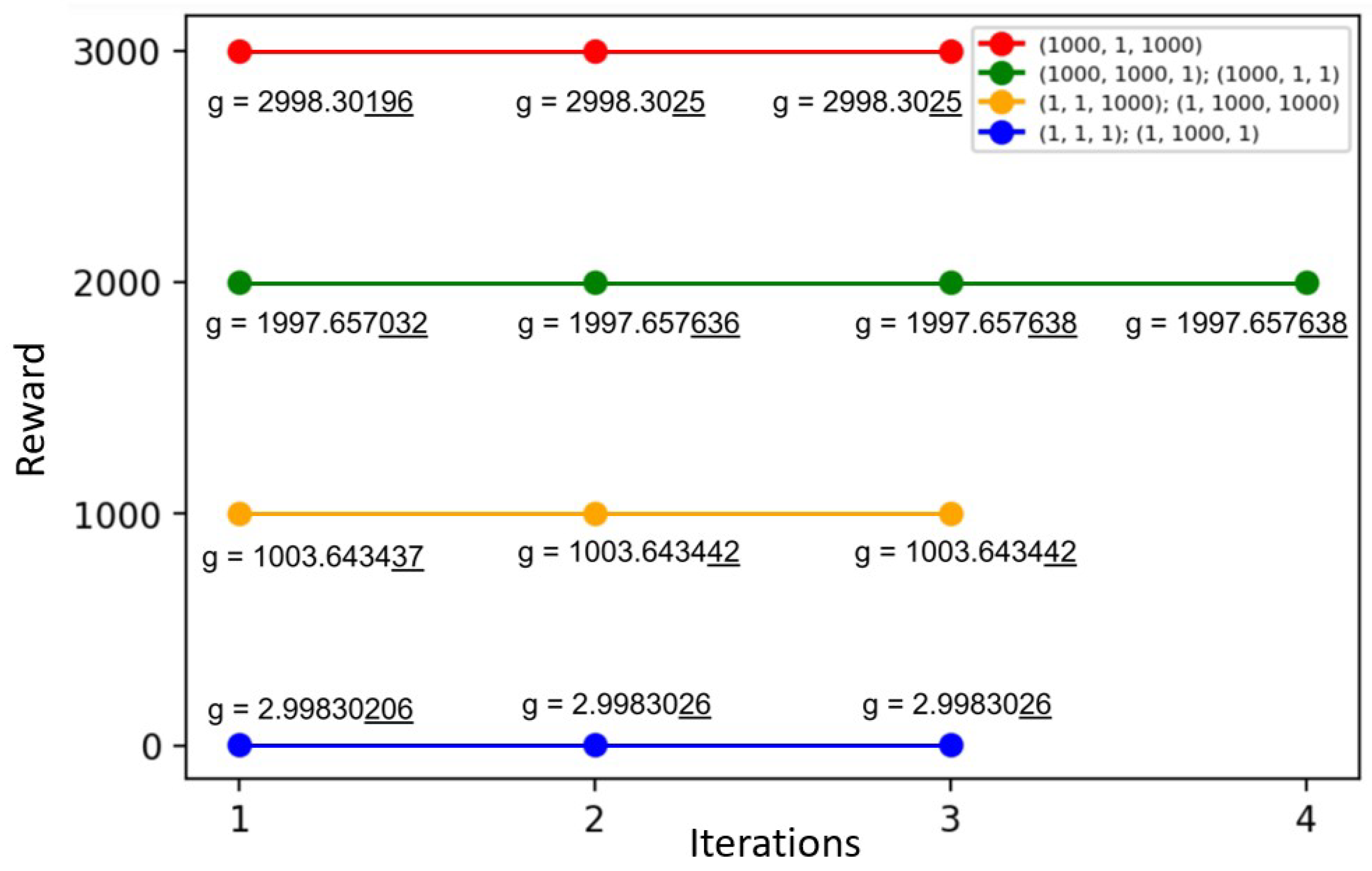
Thus, the iterative algorithm for calculating the optimal policy is summarized in Algorithm 1. The primary benefit of this algorithm, when compared with a straightforward brute force approach, lies in its computational complexity and the reduced number of iterations necessary to ascertain the optimal policy. The brute force technique’s computational complexity is contingent upon the dimensions of the set of admissible policies for each state within the system. Moreover, the convergence rate of the iterative algorithm is contingent upon the judicious selection of the initial solution. We adopt the baseline algorithm, previously discussed, as this initial solution. This algorithm aligns with one of the resource reallocation tenets, specifically the principle of maximum resource utilization. Subsequent demonstration will reveal that by employing this approach, the optimal policy can be achieved in merely three iterations.
| Algorithm 1 Policy iteration algorithm. |
- 1:
- 2:
- 3:
by Formula ( 2) ▹ Baseline algorithm - 4:
- 5:
by Formula ( 6) ▹ Policy improvement - 6:
if then return - 7:
, go to step 5 - 8:
end if
|
6. Numerical Results
In this section, we present various metrics of interest and analyze the impact of weights on the optimal policy, as well as the relationship between reward and the number of iterations in the policy iteration algorithm.
6.1. Considered Scenarios
We focus on evaluating the performance of two specific services, namely, web browsing and bulk data transfer. The numerical parameters for each service can be found in
Table 6. The recommended delay time (
) and allowable delay time (
) for data transfer are utilized to estimate the minimum-bit-rate guarantee (
b) and the abandonment rate due to impatience of users in buffers (
). The total bit rate for all network slice resources is calculated based on the chosen bandwidth, modulation and coding scheme (MCS), and MIMO scheme.
6.2. Impact of Weights on Policy
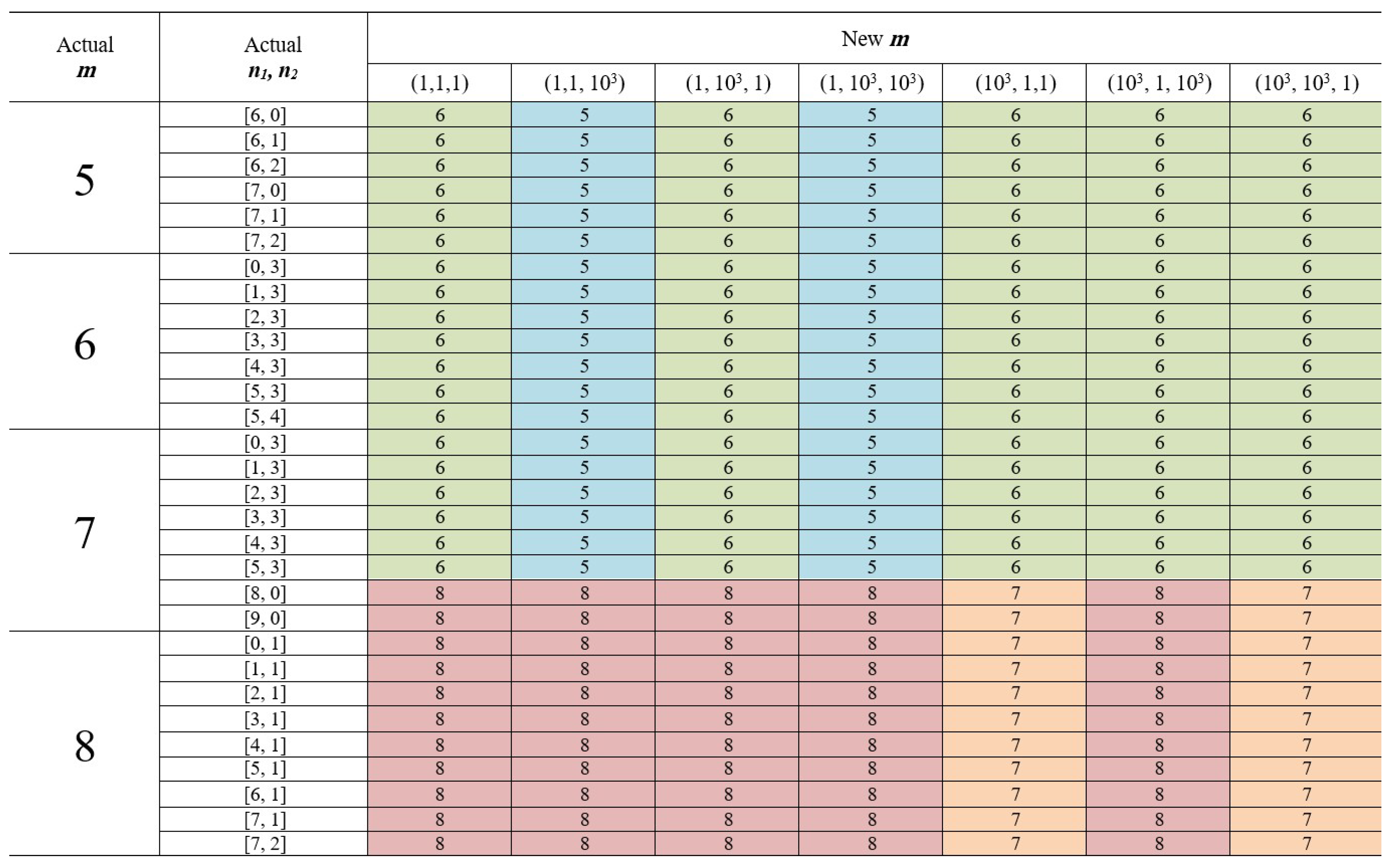
Consider a fragment of the policy for different weights in the reward function.
Figure 7 illustrates that for a fixed set of weights, and policy
m (size of 1-slice) varies depending on system states. Moreover, the policy is also influenced by the specific set of weights. The provider modifies the weighting according to their prioritization. In scenarios where all parameters are equivalent in value, uniform weights are allocated, exemplified by
. Conversely, should a particular criterion—such as one of three fundamental principles—be deemed more pivotal, its associated weight is augmented. For example, should the optimization of resource utilization take precedence, the weight distribution might be adjusted to
.
Let us examine a specific state , assuming that . In this state, six units of resources have been reallocated for the 1-slice; there are users in the 1-buffer; and the size of the 2-slice is 2, with one user in the buffer. If all weights in the set are equal, there is no change in the policy (no reallocation occurs). However, with set , where the weight corresponding to the principle of maximum resource utilization is given the highest importance, reallocation does occur: the resource of the 1-slice is reduced by 1, and a user from the 2-buffer is processed. This same scenario also applies to set .
6.3. Reward and Number of Iterations
The brute force method is not a suitable solution for finding the optimal policy. Instead, the iterative algorithm developed by R.A. Howard can be used, which allows for the determination of the optimal policy in fewer iterations. When using this algorithm, it is necessary to set a termination condition, which, in this case, is the stabilization of both the policy and the reward values. The baseline algorithm can be selected to start the algorithm, as it maximizes resource utilization. The choice of the baseline algorithm affects the number of iterations required to find a solution, as it aligns with one of the considered reallocation principles. The optimal policy should also correspond to the highest reward value. As shown in
Figure 8, the optimal policy was achieved after only three iterations, with the reward increasing with each iteration.
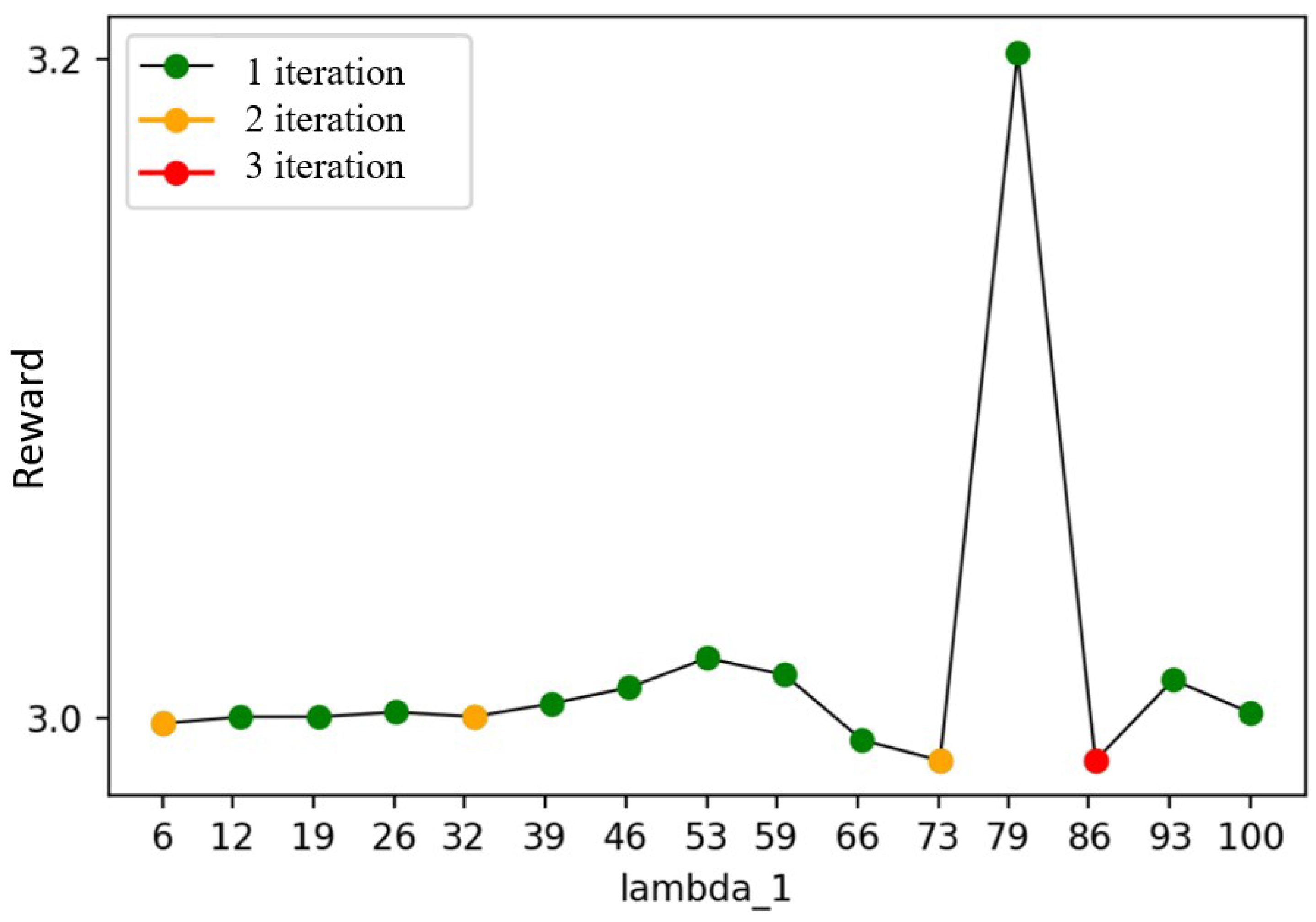
In certain scenarios, the optimal policy may not be unique and may periodically overlap. In such cases, any of these policies can be selected, as long as it results in the maximum reward and stabilization. It is important to note that the chosen policy is also influenced by the system’s parameters. Different parameter values lead to varying rewards, iterations, and types of policies. As illustrated in
Figure 9, we examined the impact of arrival rate
of requests from 1-users on a fixed set of reward function weights
.
6.4. Metrics of Interest
If a reward function is necessary for comparing policies, performance metrics are more important for providers. We considered characteristics from the provider’s perspective rather than the user’s perspective, such as the average number of requests in the buffer and the average waiting time. These characteristics include the probability (
) of resource reallocation if a signal arrives and the coefficient (
) of resource utilization. These coefficients have the same meaning as the weights in the reward function (the second and third terms, respectively).
where
,
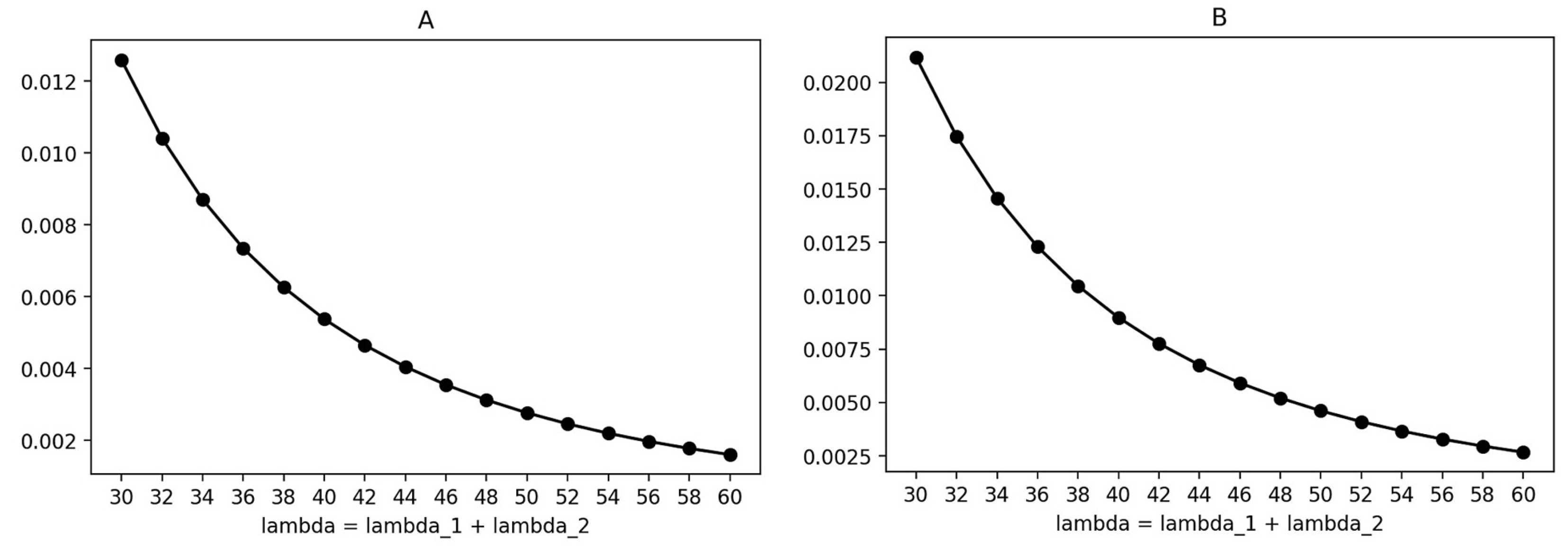
Figure 10 illustrates the graphs for the coefficient (
of resource reallocation for a fixed set of reward function weights
. Since the baseline algorithm prioritizes maximum resource utilization over the resulting reallocation, its coefficient is lower than that of the optimal policy, which considers all principles equally. As the arrival rate of requests increases, there are fewer vacancies in the buffer and fewer resources available for data transfer. However, it is not possible to increase the total size of both slices; only the size of the
k-slice can be changed by “moving the boundary”. Therefore, in this scenario, the resulting resource reallocation decreases due to fewer states where “moving the boundary” is necessary.
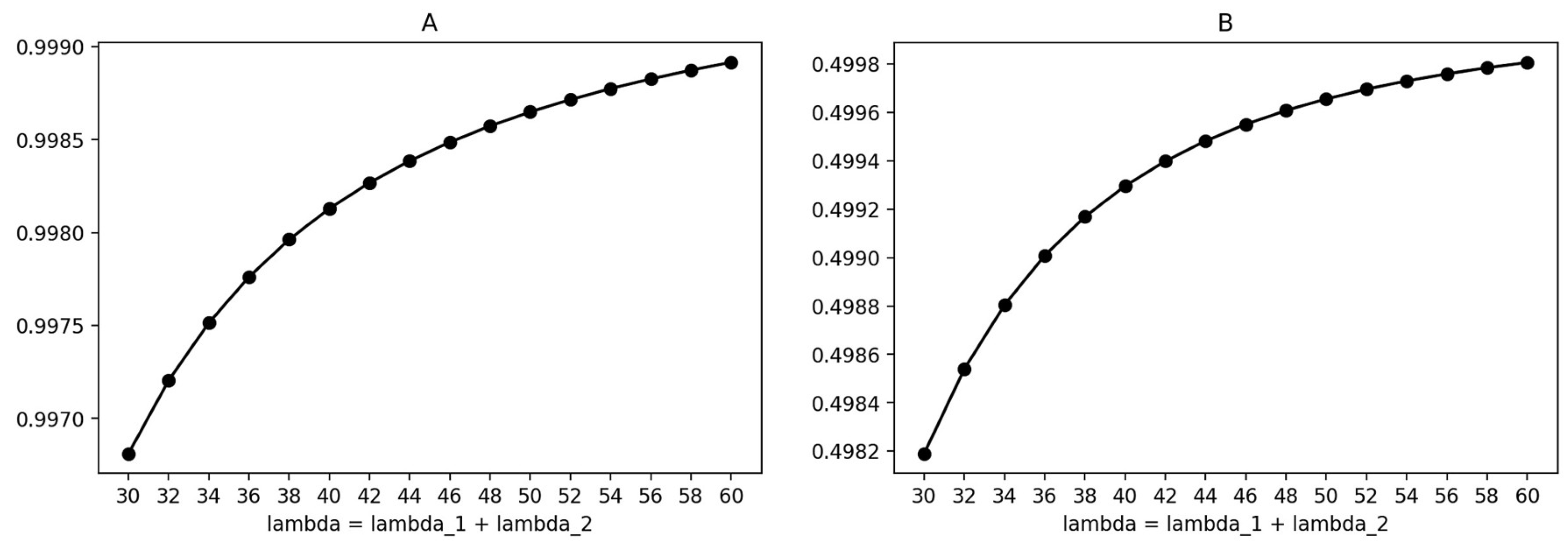
Figure 11 displays the graphs for the resource utilization coefficient (
) for a fixed set of reward function weights
. As the baseline algorithm aims for maximum resource utilization, its coefficient is close to one. However, the optimal policy considers multiple principles simultaneously, resulting in a coefficient of approximately half the size. With an increase in the arrival rate of requests, a larger slice size is needed, causing the coefficient to increase.
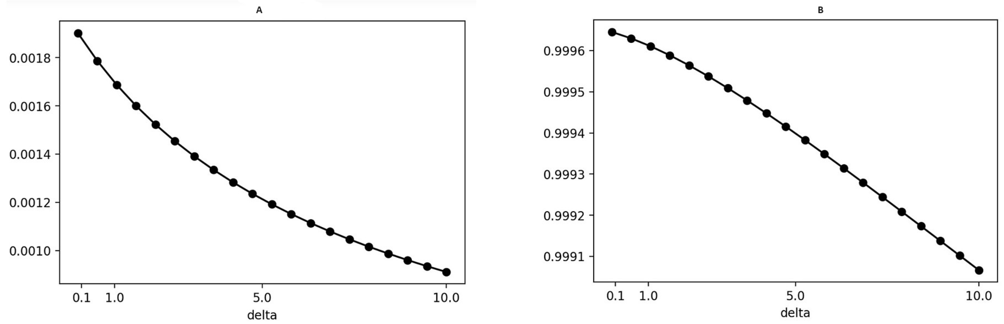
Figure 12 illustrates the relationship between the coefficients in question and the rate of signals (
) from the controller in the context of the baseline algorithm. The graphical data indicate that an increase in signal reception frequency correlates with a reduced necessity for adjusting the boundary between slices. Concurrently, although there is a reduction in the characteristic of resource utilization, its magnitude remains appreciably high.
6.5. Discussion and Future Research: Model Modifications
Expanding this model to encompass additional slices results in a stochastic process characterized by states
, with
K denoting the total number of slices. However, this expansion necessitates the derivation of the optimal policy to manage resources effectively. The efficiency of resource allocation thus becomes a critical concern. The formulation of the optimal resource allocation strategy, represented by
, is essential to enhancing system performance. As the number of slices grows, so does the complexity of the state space and the array of potential policies, potentially leading to increased computational demands and iteration counts to reach a solution. Moreover, selecting an appropriate initial policy becomes more challenging. It is crucial to acknowledge that with a rising number of service providers, the foundational algorithm previously discussed cannot be directly implemented. But the idea from paper [
50] could be used.
Addressing the limitations of our system model, we incorporate elastic traffic, which assumes that data volume requirements are parameters, whereas real-time streaming traffic relies on user-determined service durations. In such a case, the transition rate matrix, , would require modification. Regarding IoT services, the applicability of our model is contingent upon the specific service type. For instance, if the service involves sensors transmitting data where volume—not transmission time—is important, then our model is applicable.
Beyond the Poisson arrival process, alternative processes such as MAP and BMAP offer more complex structures that enable queuing systems to adjust to variable traffic loads dynamically. It is pertinent to note that while Poisson processes represent a simpler flow type, MAP can be viewed as a subset of BMAP; BMAP allows for multiple simultaneous arrivals.
This model can also be examined under dynamic conditions within a stochastic environment. For example, considering a controller’s operational status—functional or non-functional—within the framework of an unreliable system is pertinent. To account for factors such as communication channel conditions or the distance between a base station and a user, one must employ resource queuing system methodologies.
6.6. Discussion and Future Research: Computing Optimal Policy
It is important to recognize that assigning uniform weights within the reward function does not necessarily ensure the maximization of all three principles simultaneously, as conflicts may arise among them. For instance, certain scenarios may preclude the possibility of optimizing resource utilization while achieving equitable resource distribution across slices. The dynamics of their interplay warrant closer examination in future research.
Beyond the brute force approach and Howard’s iterative algorithm, alternative methods exist for finding solutions, such as neural networks. Additional techniques include linear and nonlinear programming, the asymptotic optimization method, and dynamic programming. A comparative analysis of these methods against the iterative algorithm could be beneficial in discerning their respective strengths and weaknesses.
The solutions derived with the MDP are inherently contingent on the initial parameters. An area of ongoing investigation is the robustness of these solutions to variations in the initial data. This could involve identifying parameter ranges associated with specific albeit not necessarily optimal policies that remain satisfactory.
Furthermore, future studies will aim to broaden the numerical analysis by exploring the determination of optimal policies using neural networks. This strategy would entail using the system’s current state as input to generate the policy as output. When employing neural networks, it is crucial to consider computational demands and model intricacy. Selecting an appropriate optimizer and compiling a suitable training dataset may present challenges. Nevertheless, it is hypothesized that neural networks could yield swifter solutions for extensive datasets compared with iterative methods.
7. Conclusions
In this paper, we investigate the technology of network slicing using a controllable queuing system with elastic traffic, motivated by the desire to utilize network resources more efficiently. We construct a system model for one network slice provider and two network slice service providers. An iterative algorithm is used to implement the required model in order to find the optimal policy for resource reallocation. This method allows for faster results compared with the brute force approach. Additionally, the principles guiding resource reallocation are determined and include maximum matching for equal resource partitioning, maximum share of the signals resulting in resource reallocation, and maximum resource utilization.
The numerical results obtained indicate that the optimal policy depends on several factors, including the current state of the system and the ratio between the weights in the reward function. Furthermore, the choice of the initial reallocation based on one of the principles is also significant. In our case, the initial reallocation was correctly chosen to correspond to the maximum resource utilization, leading to a solution being found in fewer iterations. We also explored the performance indicators, such as the coefficient of resulting resource reallocation and the resource utilization coefficient. The obtained results indicate that the optimal policy obtained using the constructed model is effective compared with the initial one.
Author Contributions
Conceptualization, project administration, supervision, methodology, writing—review and editing, I.K. and K.S.; formal analysis, investigation, A.V. and S.B.; software, validation, visualization, writing—original draft, K.L., I.G. and A.K. All authors have read and agreed to the published version of the manuscript.
Funding
This publication was supported by the RUDN University Scientific Projects Grant System, project No. 025319-2-000.
Data Availability Statement
The data presented in this study are available in this article.
Conflicts of Interest
The authors declare no conflicts of interest.
Abbreviations
The following abbreviations are used in this manuscript:
| 5G | Fifth generation |
| 6G | Sixth generation |
| BMAP | Batch Markovian arrival process |
| CTMC | Continuous-time Markov chain |
| DQN | Deep Q-network |
| DRL | Deep reinforcement learning |
| eMBB | Enhanced mobile broadband |
| GBR | Guaranteed bit rate |
| IoT | Internet of Things |
| MAP | Markovian arrival process |
| MCS | Modulation and coding scheme |
| MDP | Markov decision process |
| MIMO | Multiple input multiple output |
| ML | Machine learning |
| mMTC | Massive machine-type communications |
| MNO | Mobile network operator |
| MVNO | Mobile virtual network operator |
| QoS | Quality of service |
| QPSK | Quadrature phase-shift keying |
| RL | Reinforcement learning |
| SLA | Service-level agreement |
| URLLC | Ultra-reliable low-latency communication |
| V2X | Vehicle to everything |
| VNF | Virtualized network function |
References
- Moltchanov, D.; Sopin, E.; Begishev, V.; Samuylov, A.; Koucheryavy, Y.; Samouylov, K. A Tutorial on Mathematical Modeling of 5G/6G Millimeter Wave and Terahertz Cellular Systems. IEEE Commun. Surv. Tutor. 2022, 24, 1072–1116. [Google Scholar] [CrossRef]
- Kochetkov, D.; Vuković, D.; Sadekov, N.; Levkiv, H. Smart Cities and 5G Networks: An Emerging Technological Area? J. Geogr. Inst. Jovan Cvijic SASA 2019, 69, 289–295. [Google Scholar] [CrossRef]
- Kochetkov, D.; Almaganbetov, M. Using Patent Landscapes for Technology Benchmarking: A Case of 5G Networks. Adv. Syst. Sci. Appl. 2021, 21, 20–28. [Google Scholar] [CrossRef]
- Popovski, P.; Trillingsgaard, K.F.; Simeone, O.; Durisi, G. 5G Wireless Network Slicing for eMBB, URLLC, and mMTC: A Communication-Theoretic View. IEEE Access 2018, 6, 55765–55779. [Google Scholar] [CrossRef]
- Giordani, M.; Polese, M.; Mezzavilla, M.; Rangan, S.; Zorzi, M. Toward 6G Networks: Use Cases and Technologies. IEEE Commun. Mag. 2020, 58, 55–61. [Google Scholar] [CrossRef]
- Duan, X.D.; Wang, X.Y.; Lu, L.; Shi, N.X.; Liu, C.; Zhang, T.; Sun, T. 6G Architecture Design: From Overall, Logical and Networking Perspective. IEEE Commun. Mag. 2023, 61, 158–164. [Google Scholar] [CrossRef]
- Dangi, R.; Jadhav, A.; Choudhary, G.; Dragoni, N.; Mishra, M.K.; Lalwani, P. ML-Based 5G Network Slicing Security: A Comprehensive Survey. Future Internet 2022, 14, 116. [Google Scholar] [CrossRef]
- Hu, Y.; Gong, L.; Li, X.; Li, H.; Zhang, R.; Gu, R. A Carrying Method for 5G Network Slicing in Smart Grid Communication Services Based on Neural Network. Future Internet 2023, 15, 247. [Google Scholar] [CrossRef]
- 3rd Generation Partnership Project (3GPP). Charging Management; Study on Charging Aspects of Network Slicing. Technical Report 3GPP 32.845. January 2020. Available online: https://portal.3gpp.org/desktopmodules/Specifications/SpecificationDetails.aspx?specificationId=3583 (accessed on 1 November 2023).
- ITU-T. Framework for the Support of Network Slicing in the IMT-2020 Network. Recommendation ITU-T Y.3112. December 2018. Available online: https://www.itu.int/rec/T-REC-Y.3112-201812-I (accessed on 1 November 2023).
- ITU-T. Requirements of the IMT-2020 Network. Recommendation ITU-T Y.3101. 2018. Available online: https://www.itu.int/rec/T-REC-Y.3101-201801-I (accessed on 1 November 2023).
- Lieto, A.; Malanchini, I.; Capone, A. Enabling Dynamic Resource Sharing for Slice Customization in 5G Networks. In Proceedings of the 2018 IEEE Global Communications Conference, GLOBECOM 2018, Abu Dhabi, United Arab Emirates, 9–13 December 2018. [Google Scholar] [CrossRef]
- Khatibi, S. Radio Resource Management Strategies in Virtual Networks. Ph.D. Thesis, IST—University of Lisbon, Lisbon, Portugal, 2016. Available online: https://grow.tecnico.ulisboa.pt/wp-content/uploads/2016/08/Thesis_sina_khatibi_IST172360.pdf (accessed on 1 November 2023).
- Bega, D.; Gramaglia, M.; Banchs, A.; Sciancalepore, V.; Costa-Perez, X. A Machine Learning Approach to 5G Infrastructure Market Optimization. IEEE Trans. Mob. Comput. 2020, 19, 498–512. [Google Scholar] [CrossRef]
- Garcia-Morales, J.; Lucas-Estan, M.C.; Gozalvez, J. Latency-Sensitive 5G RAN Slicing for Industry 4.0. IEEE Access 2019, 7, 143139–143159. [Google Scholar] [CrossRef]
- Papa, A.; Klugel, M.; Goratti, L.; Rasheed, T.; Kellerer, W. Optimizing Dynamic RAN Slicing in Programmable 5G Networks. In Proceedings of the 2019 IEEE International Conference on Communications, ICC 2019, Shanghai, China, 20–24 May 2019; Volume 2019. [Google Scholar] [CrossRef]
- Zhou, G.; Zhao, L.; Liang, K.; Zheng, G.; Hanzo, L. Utility Analysis of Radio Access Network Slicing. IEEE Trans. Veh. Technol. 2020, 69, 1163–1167. [Google Scholar] [CrossRef]
- Vila, I.; Sallent, O.; Umbert, A.; Perez-Romero, J. An Analytical Model for Multi-Tenant Radio Access Networks Supporting Guaranteed Bit Rate Services. IEEE Access 2019, 7, 57651–57662. [Google Scholar] [CrossRef]
- Vo, P.L.; Nguyen, M.N.; Le, T.A.; Tran, N.H. Slicing the Edge: Resource Allocation for RAN Network Slicing. IEEE Wirel. Commun. Lett. 2018, 7, 970–973. [Google Scholar] [CrossRef]
- Sun, Y.; Qin, S.; Feng, G.; Zhang, L.; Imran, M.A. Service Provisioning Framework for RAN Slicing: User Admissibility, Slice Association and Bandwidth Allocation. IEEE Trans. Mob. Comput. 2021, 20, 3409–3422. [Google Scholar] [CrossRef]
- Zhao, G.; Qin, S.; Feng, G.; Sun, Y. Network Slice Selection in Softwarization-Based Mobile Networks. Trans. Emerg. Telecommun. Technol. 2020, 31, e3617. [Google Scholar] [CrossRef]
- Khatibi, S.; Correia, L.M. Modelling Virtual Radio Resource Management in Full Heterogeneous Networks. Eurasip J. Wirel. Commun. Netw. 2017, 2017, 73. [Google Scholar] [CrossRef]
- Marabissi, D.; Fantacci, R. Highly Flexible RAN Slicing Approach to Manage Isolation, Priority, Efficiency. IEEE Access 2019, 7, 97130–97142. [Google Scholar] [CrossRef]
- Lee, Y.L.; Loo, J.; Chuah, T.C.; Wang, L.C. Dynamic Network Slicing for Multitenant Heterogeneous Cloud Radio Access Networks. IEEE Trans. Wirel. Commun. 2018, 17, 2146–2161. [Google Scholar] [CrossRef]
- Akgul, O.U.; Malanchini, I.; Capone, A. Dynamic Resource Trading in Sliced Mobile Networks. IEEE Trans. Netw. Serv. Manag. 2019, 16, 220–233. [Google Scholar] [CrossRef]
- Tun, Y.K.; Tran, N.H.; Ngo, D.T.; Pandey, S.R.; Han, Z.; Hong, C.S. Wireless Network Slicing: Generalized Kelly Mechanism-Based Resource Allocation. IEEE J. Sel. Areas Commun. 2019, 37, 1794–1807. [Google Scholar] [CrossRef]
- Caballero, P.; Banchs, A.; De Veciana, G.; Costa-Perez, X. Network Slicing Games: Enabling Customization in Multi-Tenant Mobile Networks. IEEE/ACM Trans. Netw. 2019, 27, 662–675. [Google Scholar] [CrossRef]
- Caballero, P.; Banchs, A.; De Veciana, G.; Costa-Perez, X.; Azcorra, A. Network Slicing for Guaranteed Rate Services: Admission Control and Resource Allocation Games. IEEE Trans. Wirel. Commun. 2018, 17, 6419–6432. [Google Scholar] [CrossRef]
- Ksentini, A.; Nikaein, N. Toward Enforcing Network Slicing on RAN: Flexibility and Resources Abstraction. IEEE Commun. Mag. 2017, 55, 102–108. [Google Scholar] [CrossRef]
- Kokku, R.; Mahindra, R.; Zhang, H.; Rangarajan, S. CellSlice: Cellular Wireless Resource Slicing for Active RAN Sharing. In Proceedings of the 2013 5th International Conference on Communication Systems and Networks, COMSNETS 2013, Bangalore, India, 7–10 January 2013. [Google Scholar] [CrossRef]
- Parsaeefard, S.; Dawadi, R.; Derakhshani, M.; Le-Ngoc, T. Joint User-Association and Resource-Allocation in Virtualized Wireless Networks. IEEE Access 2016, 4, 2738–2750. [Google Scholar] [CrossRef]
- Narmanlioglu, O.; Zeydan, E.; Arslan, S.S. Service-Aware Multi-Resource Allocation in Software-Defined Next Generation Cellular Networks. IEEE Access 2018, 6, 20348–20363. [Google Scholar] [CrossRef]
- Yan, M.; Feng, G.; Zhou, J.; Sun, Y.; Liang, Y.C. Intelligent Resource Scheduling for 5G Radio Access Network Slicing. IEEE Trans. Veh. Technol. 2019, 68, 7691–7703. [Google Scholar] [CrossRef]
- Moskaleva, F.; Lisovskaya, E.; Lapshenkova, L.; Shorgin, S.; Gaidamaka, Y. Example of Degrading Network Slicing System in Two-Service Retrial Queueing System. Lect. Notes Comput. Sci. 2021, 13144, 79–293. [Google Scholar] [CrossRef]
- Mazumdar, R.; Mason, L.G.; Douligeris, C. Fairness in Network Optimal Flow Control: Optimality of Product Forms. IEEE Trans. Commun. 1991, 39, 775–782. [Google Scholar] [CrossRef]
- Malanchini, I.; Valentin, S.; Aydin, O. Wireless Resource Sharing for Multiple Operators: Generalization, Fairness, and the Value of Prediction. Comput. Netw. 2016, 100, 110–123. [Google Scholar] [CrossRef]
- Sánchez, J.A.H.; Casilimas, K.; Rendon, O.M.C. Deep Reinforcement Learning for Resource Management on Network Slicing: A Survey. Sensors 2022, 22, 3031. [Google Scholar] [CrossRef] [PubMed]
- Markova, E.; Adou, Y.; Ivanova, D.; Golskaia, A.; Samouylov, K. Queue with Retrial Group for Modeling Best Effort Traffic with Minimum Bit Rate Guarantee Transmission Under Network Slicing. Lect. Notes Comput. Sci. 2019, 11965, 432–442. [Google Scholar] [CrossRef]
- Ageev, K.; Sopin, E.; Samouylov, K. Resource Sharing Model with Minimum Allocation for the Performance Analysis of Network Slicing. Commun. Comput. Inf. Sci. 2021, 1391, 378–389. [Google Scholar] [CrossRef]
- Nassar, A.; Yilmaz, Y. Deep Reinforcement Learning for Adaptive Network Slicing in 5G for Intelligent Vehicular Systems and Smart Cities. IEEE Internet Things J. 2022, 9, 222–235. [Google Scholar] [CrossRef]
- Ou, R.; Sun, G.; Ayepah-Mensah, D.; Boateng, G.O.; Liu, G. Two-Tier Resource Allocation for Multitenant Network Slicing: A Federated Deep Reinforcement Learning Approach. IEEE Internet Things J. 2023, 10, 20174–20187. [Google Scholar] [CrossRef]
- Ou, R.; Boateng, G.O.; Ayepah-Mensah, D.; Sun, G.; Liu, G. Stackelberg game-based dynamic resource trading for network slicing in 5G networks. J. Netw. Comput. Appl. 2023, 214, 103600. [Google Scholar] [CrossRef]
- Xiao, D.; Chen, S.; Ni, W.; Zhang, J.; Zhang, A.; Liu, R. A sub-action aided deep reinforcement learning framework for latency-sensitive network slicing. Comput. Netw. 2022, 217, 109279. [Google Scholar] [CrossRef]
- Kim, Y.; Lim, H. Multi-Agent Reinforcement Learning-Based Resource Management for End-to-End Network Slicing. IEEE Access 2021, 9, 56178–56190. [Google Scholar] [CrossRef]
- Filali, A.; Mlika, Z.; Cherkaoui, S.; Kobbane, A. Dynamic SDN-Based Radio Access Network Slicing With Deep Reinforcement Learning for URLLC and eMBB Services. IEEE Trans. Netw. Sci. Eng. 2022, 9, 2174–2187. [Google Scholar] [CrossRef]
- Kim, Y.; Kim, S.; Lim, H. Reinforcement learning based resource management for network slicing. Appl. Sci. 2019, 9, 2361. [Google Scholar] [CrossRef]
- Wang, W.; Tang, L.; Liu, T.; He, X.; Liang, C.; Chen, Q. Towards Reliability-Enhanced, Delay-Guaranteed Dynamic Network Slicing: A Multi-Agent DQN Approach with An Action Space Reduction Strategy. IEEE Internet Things J. 2023. [Google Scholar] [CrossRef]
- Vlaskina, A.; Polyakov, N.; Gudkova, I. Modeling and Performance Analysis of Elastic Traffic with Minimum Rate Guarantee Transmission Under Network Slicing. Lect. Notes Comput. Sci. 2019, 11660, 621–634. [Google Scholar] [CrossRef]
- Kochetkova, I.; Vlaskina, A.; Vu, N.; Shorgin, V. Queuing System with Signals for Dynamic Resource Allocation for Analyzing Network Slicing in 5G Networks. Inform. Primen. 2021, 15, 91–97. (In Russian) [Google Scholar] [CrossRef]
- Kochetkova, I.; Vlaskina, A.; Burtseva, S.; Savich, V.; Hosek, J. Analyzing the Effectiveness of Dynamic Network Slicing Procedure in 5G Network by Queuing and Simulation Models. Lect. Notes Comput. Sci. 2020, 12525, 71–85. [Google Scholar] [CrossRef]
- Efrosinin, D.; Stepanova, N. Estimation of the Optimal Threshold Policy in a Queue with Heterogeneous Servers using a Heuristic Solution and Artificial Neural Networks. Mathematics 2021, 9, 1267. [Google Scholar] [CrossRef]
- Efrosinin, D.; Sztrik, J. An Algorithmic Approach to Analysing the Reliability of a Controllable Unreliable Queue with Two Heterogeneous Servers. Eur. J. Oper. Res. 2018, 271, 934–952. [Google Scholar] [CrossRef]
- Efrosinin, D.; Farkhadov, M.; Stepanova, N. Study of a Controllable Queueing System with Unreliable Heterogeneous Servers. Autom. Remote Control 2018, 79, 265–285. [Google Scholar] [CrossRef]
Figure 1.
Business roles related to network slicing.
Figure 1.
Business roles related to network slicing.
Figure 2.
Considered scenario.
Figure 2.
Considered scenario.
Figure 3.
Network slicing business roles in the considered scenario.
Figure 3.
Network slicing business roles in the considered scenario.
Figure 4.
General scheme of cases of resource reallocation between the service providers performed by the controller.
Figure 4.
General scheme of cases of resource reallocation between the service providers performed by the controller.
Figure 5.
Signals resulting and not resulting in resource reallocation between the service providers.
Figure 5.
Signals resulting and not resulting in resource reallocation between the service providers.
Figure 6.
Queueing system.
Figure 6.
Queueing system.
Figure 7.
Optimal policy depending on weights (different colors are associated with different numbers).
Figure 7.
Optimal policy depending on weights (different colors are associated with different numbers).
Figure 8.
Average reward vs. number of iterations to find the optimal policy.
Figure 8.
Average reward vs. number of iterations to find the optimal policy.
Figure 9.
Average reward vs. arrival rate of requests from 1-users.
Figure 9.
Average reward vs. arrival rate of requests from 1-users.
Figure 10.
Probability that if a signal arrives, this results in resource reallocation. (A) Baseline algorithm. (B) Optimal policy.
Figure 10.
Probability that if a signal arrives, this results in resource reallocation. (A) Baseline algorithm. (B) Optimal policy.
Figure 11.
Resource utilization coefficient. (A) Baseline algorithm. (B) Optimal policy.
Figure 11.
Resource utilization coefficient. (A) Baseline algorithm. (B) Optimal policy.
Figure 12.
Metrics for baseline algorithm. (A) Probability that if a signal arrives, this results in resource reallocation. (B) Resource utilization coefficient.
Figure 12.
Metrics for baseline algorithm. (A) Probability that if a signal arrives, this results in resource reallocation. (B) Resource utilization coefficient.
Table 1.
Summary of selected works on network slicing mechanisms.
Table 1.
Summary of selected works on network slicing mechanisms.
| Mechanism | Ref. |
|---|
| Network slice service planning mechanisms |
| eMBB, mMTC, and URLLC | [4,11,12] |
| Mobile virtual network operators (MVNOs) | [13] |
| Traffic type: guaranteed bit rate (GBR), non-GBR, streaming, elastic | [14] |
| Resource capacity planning mechanisms |
| Weights for services according to bit-rate or latency requirements | [12,15,16,17,18,19,20,21] |
| Service-level agreement (SLA) | [22] |
| Slice priorities | [18,23,24,25] |
| Auction model | [26,27,28] |
| Isolation to guarantee the minimum and/or maximum bit rate | [16,18,29,30,31,32,33] |
| QoS degradation | [34] |
| Three equally weighed criteria: (i) ratio of the average throughput to average delay of one user/slice; (ii) average network throughput subject to average delay constraints; (iii) barrier function | [35] |
| Three equally weighed criteria: (i) co-occurrence rate; (ii) maximum deviation; (iii) the time interval within which the deviation is possible | [36] |
Table 2.
Summary of selected works employing a Markov decision process (MDP) for resource capacity planning in network slicing.
Table 2.
Summary of selected works employing a Markov decision process (MDP) for resource capacity planning in network slicing.
| Ref. | Approaches Involving MDP | Reward Function | Action |
|---|
| [40] | Deep reinforcement learning (DRL) | Resource efficiency, edge computing performance assessment, QoS maintenance | Service request arrivals within a cluster of fog nodes overseen by an edge controller |
| [41] | Federated DRL | QoS satisfaction, network load for each MVNO | Coordinated by the InP controller |
| [42] | Multi-agent dueling deep Q-network (DQN) | Income from one transaction, net income from all transactions, benefits achieved by a user in each transaction, transaction cost generated by each transaction | An economic model initiates dynamic pricing interactions, leading to the redistribution of resources |
| [43] | Double DQN, Dijkstra algorithm, binary search-assisted gradient descent | Minimization of the number of accepted service requests with higher priority and minimization of the total cost | A double DQN-agent chooses the location for VNFs of an incoming request |
| [44] | RL, proximal policy optimization | Resource utilization, QoS violation penalty | A resource management agent monitors the status of network slices and MEC nodes and makes decisions on adjusting the allocated resources |
| [45] | Exponential weight algorithm for exploration and exploitation, multi-agent DQN | Two reward functions: (i) total achievable bit rate of URLLC and eMBB users; (ii) whether or not the agent has successfully allocated the needed resource blocks to its associated user | Every gNodeB schedules pre-allocated resource blocks assigned by the SDN controller to its associated end-users |
| [46] | DQN, RL | Maximization of slice tenant’s profit | Tenants autonomously control resource allocation and engage in negotiations with the provider to effectively manage and optimize resource utilization |
| [47] | Dynamic mixed-integer linear programming, DRL | Minimization of the total cost for VNF orchestration, backup, and mapping with delay constraints, reliability requirements, and limited resources | The resource management agent selects a random action with a certain probability for exploration and selects the best action that follows the greedy policy |
Table 3.
Main notation.
| Parameter | Description |
|---|
| Network slice provider (network operator) parameters |
| C | Total bit rate (capacity) for all network slice resources, bps |
| Number of service providers, i.e., network slices |
| Arrival rate of signals from the controller for resource reallocation between service providers, 1/s |
| Weight for maximum matching for equal resource partitioning |
| Weight for maximum share of the signals resulting in resource reallocation |
| Weight for maximum resource utilization |
| Network slice service provider (communication service provider) parameters |
| b | Minimum-bit-rate guarantee for transmitting elastic traffic, bps |
| Maximum number of all providers users jointly transmitting elastic traffic |
| Maximum number of the k-provider users (k-users) waiting for delayed elastic traffic transmission (size of k-buffer) |
| Network slice service user (communication service customer) parameters |
| Arrival rate of requests for elastic traffic transmission from k-users, 1/s |
| Average volume of elastic traffic transmitted by k-users, bit |
| Abandonment rate due to impatience of k-users in k-buffer, 1/s |
| Markov decision process (MDP) |
| m | Maximum number of 1-users jointly transmitting elastic traffic (size of 1-slice) |
| Number of 1-users transmitting elastic traffic and waiting in 1-buffer |
| Number of 2-users transmitting elastic traffic and waiting in 2-buffer |
| State of the system |
| Set of states |
| Action, i.e., size of 1-slice |
| Set of actions available from state |
| Transition rate that action a in state leads to state |
| Reward received while in state , i.e., the weighted objective with , , and |
| Markov decision process (MDP) |
Table 4.
Transition rates related to users.
Table 4.
Transition rates related to users.
| Description | Transition Rate | Condition on s | State |
|---|
| Request from 1-user has arrived | | | |
| Request from 2-user has arrived | | | |
| Traffic from 1-user has been transmitted | | | |
| Traffic from 2-user has been transmitted | | | |
| 1-User has abandoned 1-buffer | | | |
| 2-User has abandoned 2-buffer | | | |
Table 5.
Transition rates related to signals from the controller.
Table 5.
Transition rates related to signals from the controller.
| Description | Condition on s | Condition on a | State |
|---|
| 1-Slice is occupied with waiting 1-users, and 2-slice is available for all 1-users in 1-buffer | , , | | |
| 1-Slice is occupied with waiting 1-users, and 2-slice is not available for all 1-users in 1-buffer | , , | | |
| 2-Slice is occupied with waiting 2-users, 1-slice is available for all 2-users in 2-buffer | , , | | |
| 2-Slice is occupied with waiting 2-users, 1-slice is not available for all 2-users in 2-buffer | , , | | |
Table 6.
Parameters for numerical example.
Table 6.
Parameters for numerical example.
| Parameter | Description | Value (Case 1) | Value (Case 2) |
|---|
| B | Bandwidth | 5 MHz | 5 MHz |
| − | MCS | QPSK | QPSK |
| − | MIMO scheme | 2 × 2 | 2 × 2 |
| C | Total bit rate for two network slices | 10 Mbps | 8.016 Mbps |
| Arrival rate of signals from the controller | 0.000001 1/s | 0.000001 1/s |
| Weights for the reallocation principles | | |
| , | Recommended delay time | 15, 2 s | 15, 2 s |
| , | Allowable delay time | 60, 4 s | 60, 4 s |
| b | Minimum-bit-rate guarantee | 1.067 Mbps | 1.067 Mbps |
| , | Size of 1-buffer and 2-buffer | 5, 5 | 2, 2 |
| , | Arrival rate of requests from 1-users and 2-users | 0.03, 0.6 1/s | 2–10, 26–50 1/s |
| , | Average volume of traffic transmitted by 1-users and 2-users | 0.125, 0.937 Mb | 0.125, 0.937 Mb |
| , | Abandonment rate due to impatience of 1-users in 1-buffer and of 2-users in 2-buffer | 0.01, 0.25 1/s | 0.01, 0.25 1/s |
| Disclaimer/Publisher’s Note: The statements, opinions and data contained in all publications are solely those of the individual author(s) and contributor(s) and not of MDPI and/or the editor(s). MDPI and/or the editor(s) disclaim responsibility for any injury to people or property resulting from any ideas, methods, instructions or products referred to in the content. |
© 2023 by the authors. Licensee MDPI, Basel, Switzerland. This article is an open access article distributed under the terms and conditions of the Creative Commons Attribution (CC BY) license (https://creativecommons.org/licenses/by/4.0/).

.jpg)
 ,
, 


