Internet-of-Things Traffic Analysis and Device Identification Based on Two-Stage Clustering in Smart Home Environments

Abstract

Smart home environments, which consist of various Internet of Things (IoT) devices to support and improve our daily lives, are expected to be widely adopted in the near future. Owing to a lack of awareness regarding the risks associated with IoT devices and challenges in replacing or the updating their firmware, adequate security measures have not been implemented. Instead, IoT device identification methods based on traffic analysis have been proposed. Since conventional methods process and analyze traffic data simultaneously, bias in the occurrence rate of traffic patterns has a negative impact on the analysis results. Therefore, this paper proposes an IoT traffic analysis and device identification method based on two-stage clustering in smart home environments. In the first step, traffic patterns are extracted by clustering IoT traffic at a local gateway located in each smart home and subsequently sent to a cloud server. In the second step, the cloud server extracts common traffic units to represent IoT traffic by clustering the patterns obtained in the first step. Two-stage clustering can reduce the impact of data bias, because each cluster extracted in the first clustering is summarized as one value and used as a single data point in the second clustering, regardless of the occurrence rate of traffic patterns. Through the proposed two-stage clustering method, IoT traffic is transformed into time series vector data that consist of common unit patterns and can be identified based on time series representations. Experiments using public IoT traffic datasets indicated that the proposed method could identify 21 IoTs devices with an accuracy of 86.9%. Therefore, we can conclude that traffic analysis using two-stage clustering is effective for improving the clustering quality, device identification, and implementation in distributed environments.

1. Introduction

Recently, smart homes have become more popular in conjunction with the widespread use of Internet of Things (IoT) devices [1]. Consequently, IoT devices have become more integrated into our daily lives. The market size of smart homes in the world increased to 80.2 billion dollars in 2022, with expectations for continued growth. Projections indicate that the market size will grow to 338.2 billion dollars in 2030 [2]. Since users can control home appliances anytime and anywhere using applications, and products can also work autonomously based on sensing data, our daily lives have become more comfortable and efficient. However, the connection of household appliances to the internet has resulted in cyberattacks [3]. A security news site states that 1.5 billion attacks on IoT devices were reported during the first half of 2021, which is more than a 100% growth in cyberattacks compared to the first half of 2020 [4]. This indicates that IoT devices, such as computers and smartphones, can be targets of attacks; thus, adequate security measures are essential. However, measures against IoT device security have not yet been sufficiently considered owing to the difficulties of replacing devices, updating their firmware, grasping their behavior, and implementing large-scale security systems in smart home environments [5]. With the continuous increase in the number of IoT devices being used, the risk of attacks is anticipated to increase. In addition, users may find it challenging to grasp and manage all the installed IoT devices, thus potentially leaving them without awareness of any anomalies caused by cyberattacks.

The first step toward ensuring security in smart home environments is that users can grasp what kinds of IoT devices are running. For this purpose, it is important to automatically identify connected IoT devices in some way. Several methods for identifying IoT devices or their behavior based on traffic analysis using machine learning have been proposed [6,7,8,9,10,11,12,13,14]. Although these methods automatically identify IoT devices and their behavior from traffic data, they do not consider how they work in smart home environments. Furthermore, since a lot of user information is included in the communication data of IoT devices, data handling is also an important issue in ensuring security and user privacy. However, these methods process all traffic data at once. When implementing the methods in a real environment, the traffic data of IoT devices collected in a smart home will be uploaded to a cloud server. As a result, this could cause leakage of user privacy information. Therefore, in this paper, we propose IoT traffic analysis and device identification methods based on two-stage clustering for smart home environments. Here, we highlight the following three points as considerations for IoT device identification methods in smart home environments:

• The need to update the identification models: People often install new IoT devices and remove older devices from their home environments. To address such replacements and maintain proper management, it is essential to update identification models frequently, which requires periodic training. However, conventional methods implement IoT device identification with only one-time learning and do not consider the computational and communication loads owing to model updating.
• How to process traffic data: Analyzing a significant amount of traffic data simultaneously in one place can cause a heavy load on the memory and CPU, as well as interfere with the analysis. With the growing use of IoT devices, the processing of a larger amount of collected IoT traffic is required. Although collecting and analyzing traffic data on a cloud server is one solution, this approach requires sending traffic data captured in smart homes to the cloud for analysis or learning, which is unsuitable from the perspective of communication traffic and user privacy. In addition, traffic data are biased because of variations in IoT device behaviors. The biases increase in proportion to the number of device types and the amount of collected traffic data, which could negatively impact the analytical results and appropriate classification. Therefore, it is necessary to consider how to process significant amounts of traffic data appropriately when implementing this method in smart home environments. However, conventional methods typically process traffic data simultaneously.
• The range that IoT device identification targets: Most methods utilize fixed values such as the IP and MAC addresses included in traffic data to identify specific IoT devices installed in smart homes. From the perspective of security in smart homes, however, it is important to identify and grasp not only whether the appropriate IoT devices are connected but also whether they operate properly. Some conventional methods analyze IoT traffic based on communication features, such as the number of destination IP addresses, the number of protocol types, and the total amount of data. However, they only focus on features in a fixed interval. Thus, methods that do not consider the time series characteristics of IoT traffic would overlook the behavior of IoT devices, since they cannot extract features from some IoT traffic owing to the differences in communication periods.

Based on these aspects, we propose an IoT traffic analysis and device identification method based on two-stage clustering [15,16] for smart home environments. The proposed method considers a two-layer distributed traffic analysis at two locations: a gateway router installed in each smart home and a cloud server. In this paper, we verified whether two-stage clustering performs properly in both IoT traffic analysis and device identification by comparing a centralized clustering method with only a cloud server. Note that in this paper, the proposed and comparative methods were implemented on a single computer and not in a distributed environment. Consequently, we extracted the specific time series characteristics of IoT traffic using two-stage clustering at a lower cost. Moreover, we implemented an IoT device identification method based on the analytical results, which can identify 21 IoT devices with an accuracy of 86.9%. The results indicate that IoT traffic analysis with two-stage clustering is effective in improving the clustering performance, device identification, and implementation in distributed environments. Our contributions can be summarized as follows:

• We summarized the concerns regarding IoT device identification in real environments: the need to regularly update identification models, how to process traffic data, and the range of IoT device identification. Thereafter, we proposed an IoT traffic analysis and device identification method based on two-stage clustering that can be implemented in smart home environments. This study investigated whether two-stage clustering performs properly in IoT traffic analysis and device identification by comparing it with a normal centralized clustering method.
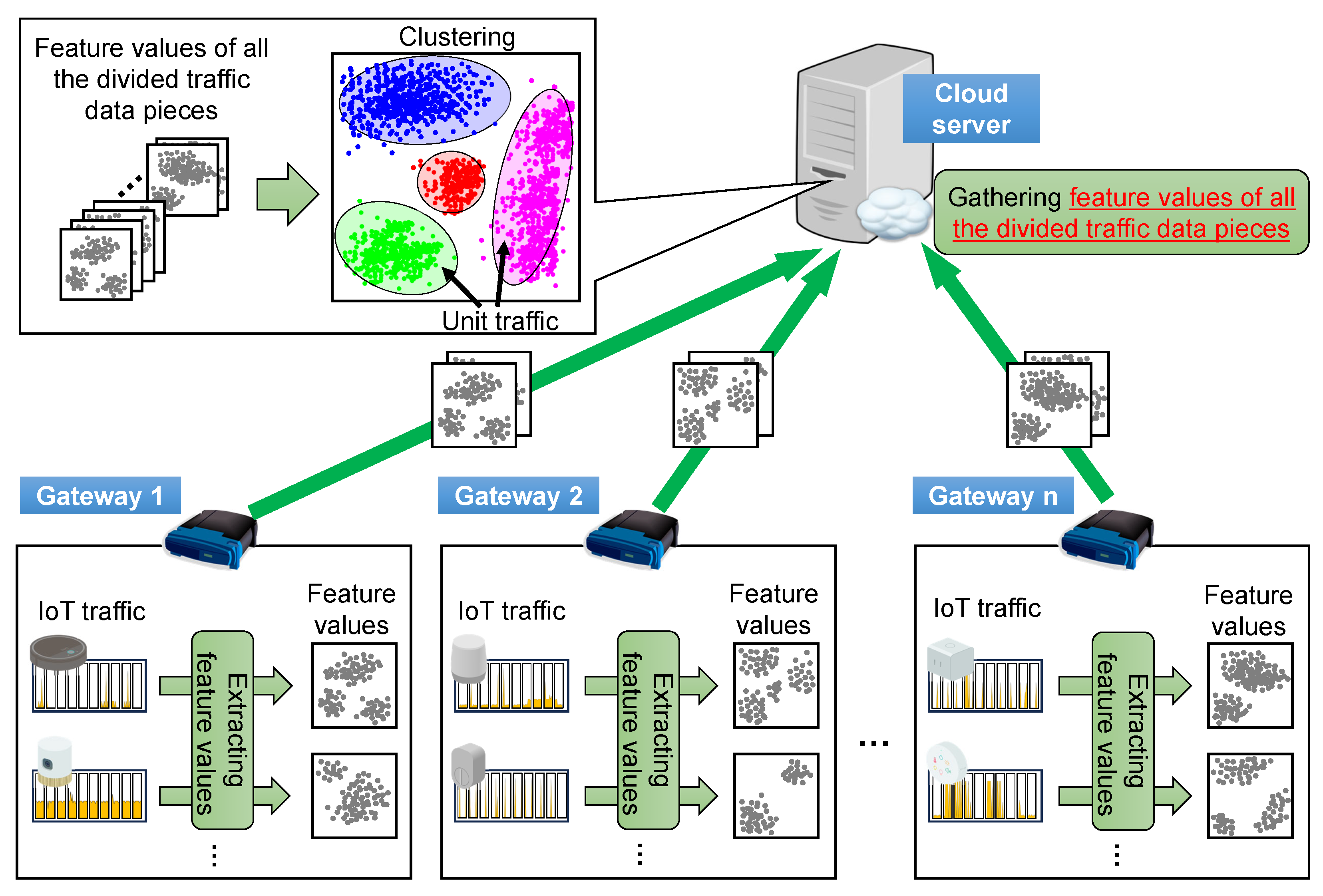
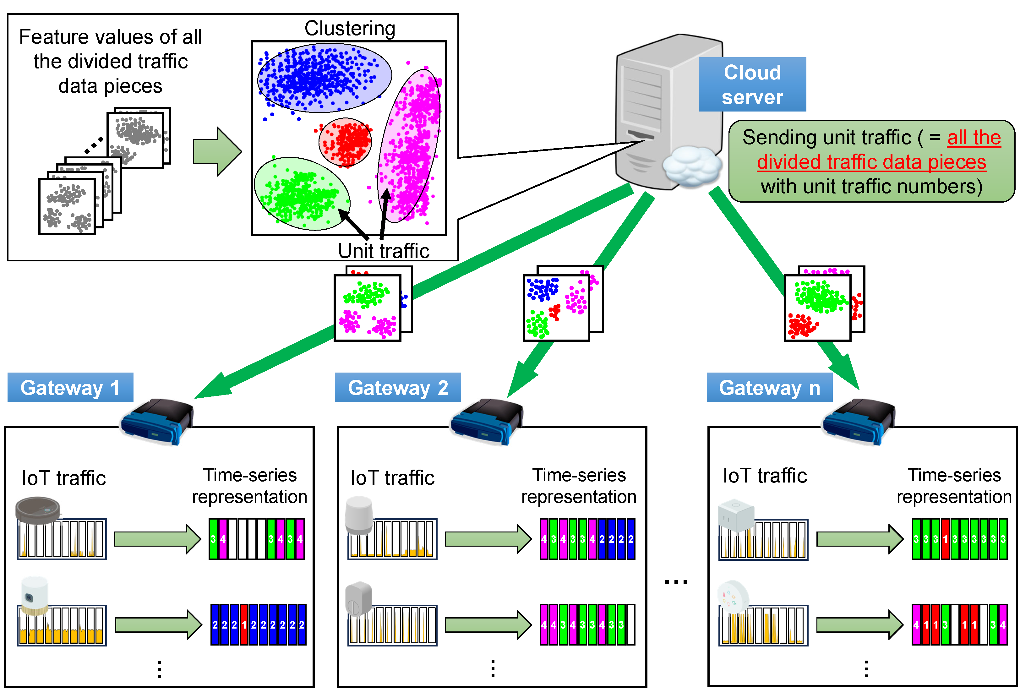
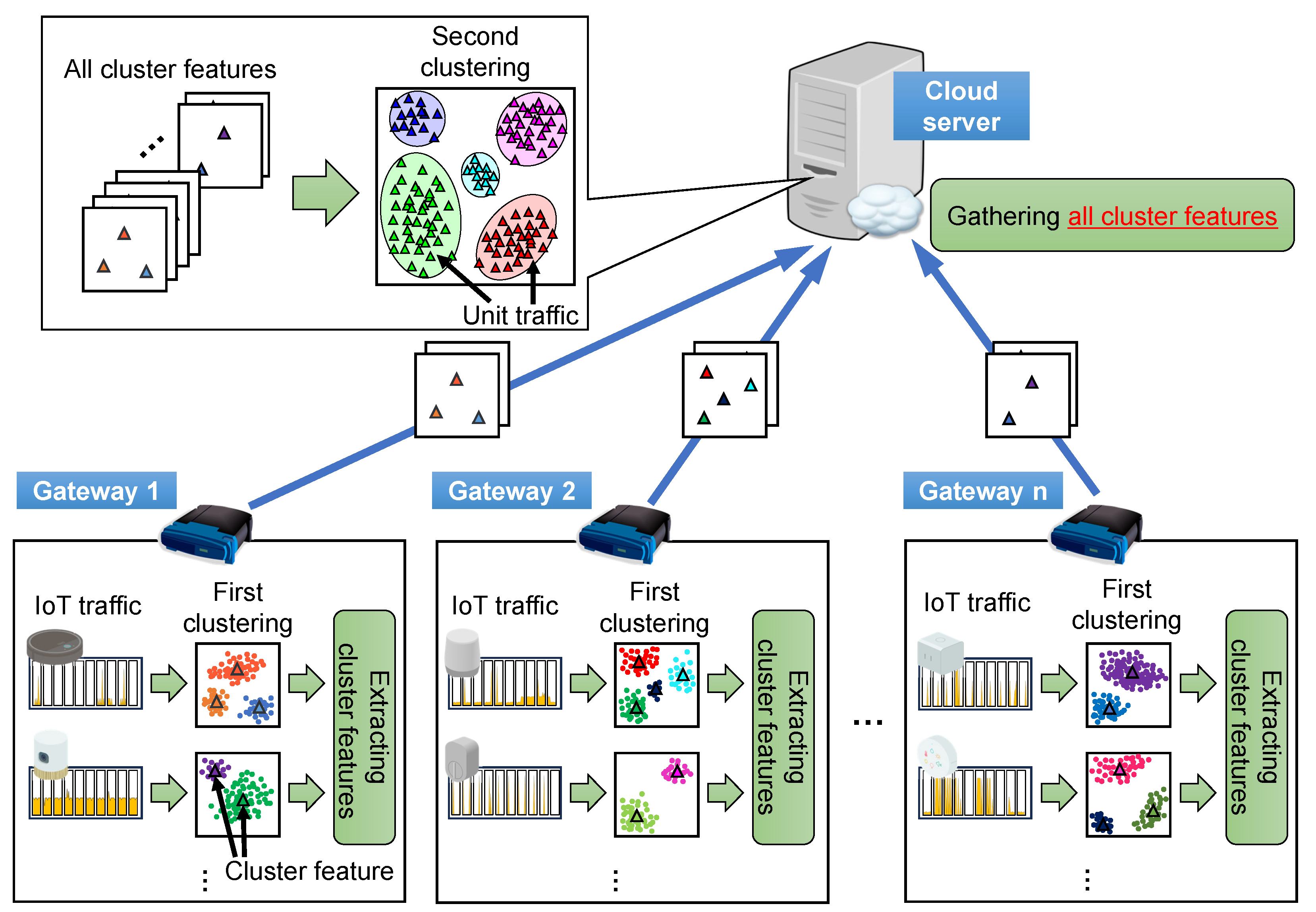
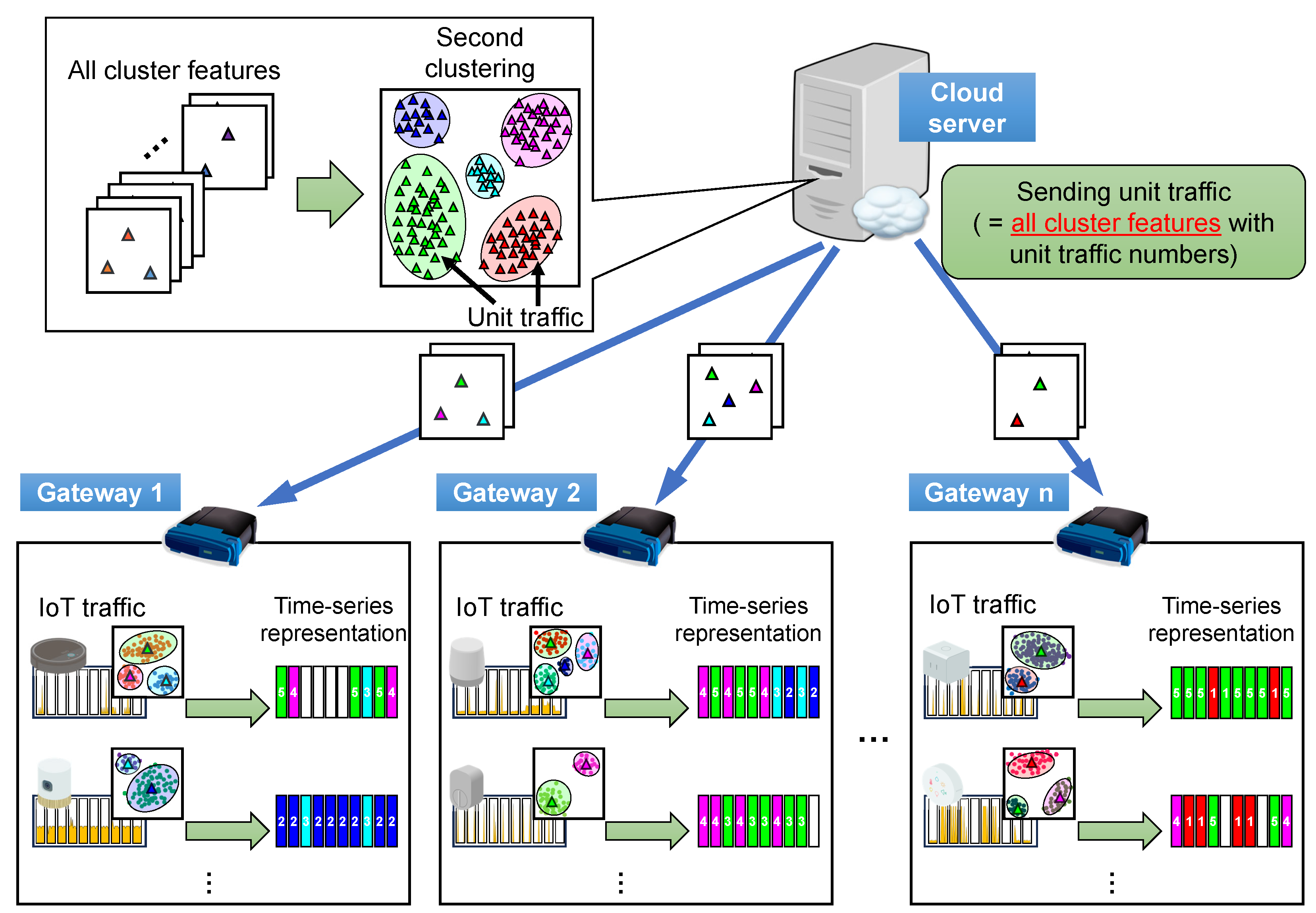
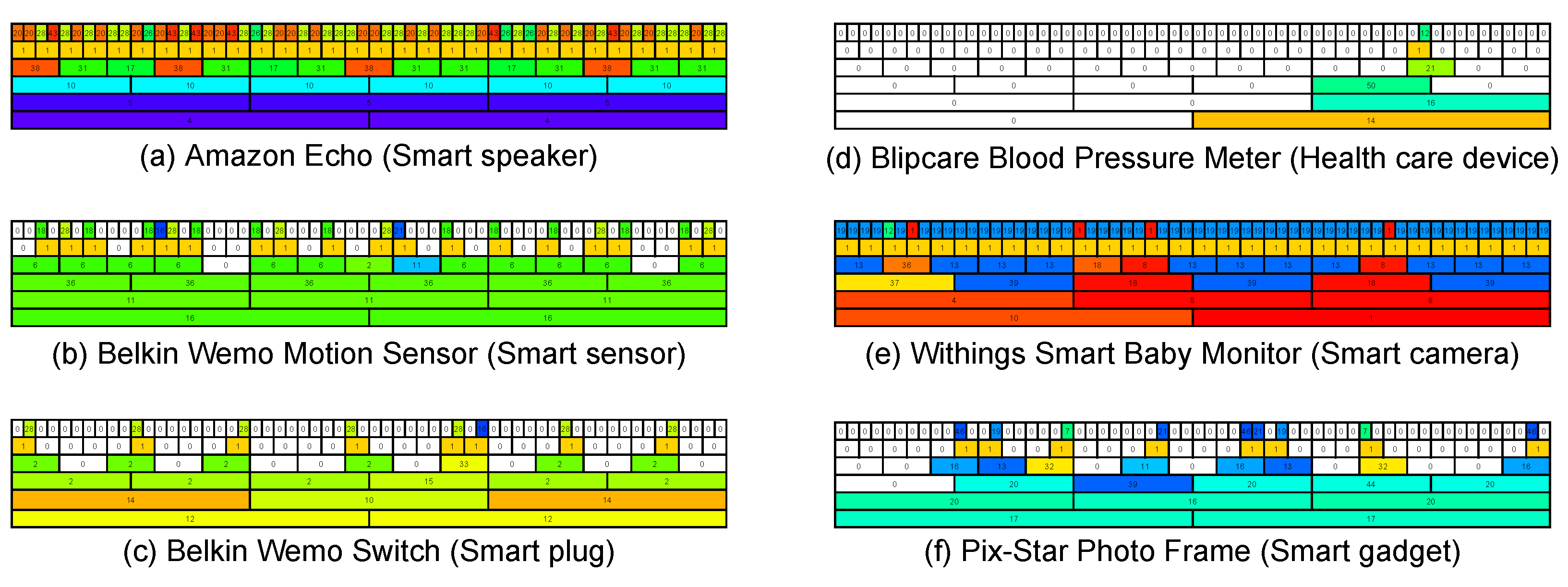
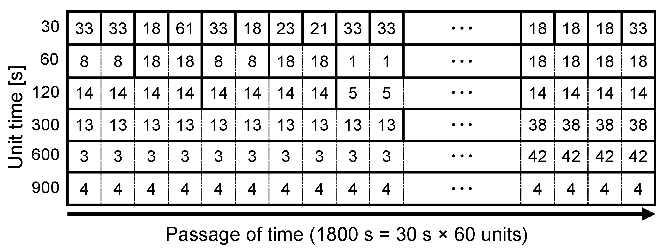
• We applied the two-stage clustering method, which has previously been proposed to grasp dynamic traffic changes specifically for peer-to-peer video streaming services (P2PTV) [15,16], to IoT traffic analysis based on the similarities between P2PTV and IoT traffic. Using two-stage clustering, we extracted traffic patterns to describe IoT traffic and transformed the IoT traffic into a time series numerical representation, which is a series of traffic patterns. Consequently, we visualized the time series characteristics of the communication of IoT devices and extracted traffic features for IoT device identification.
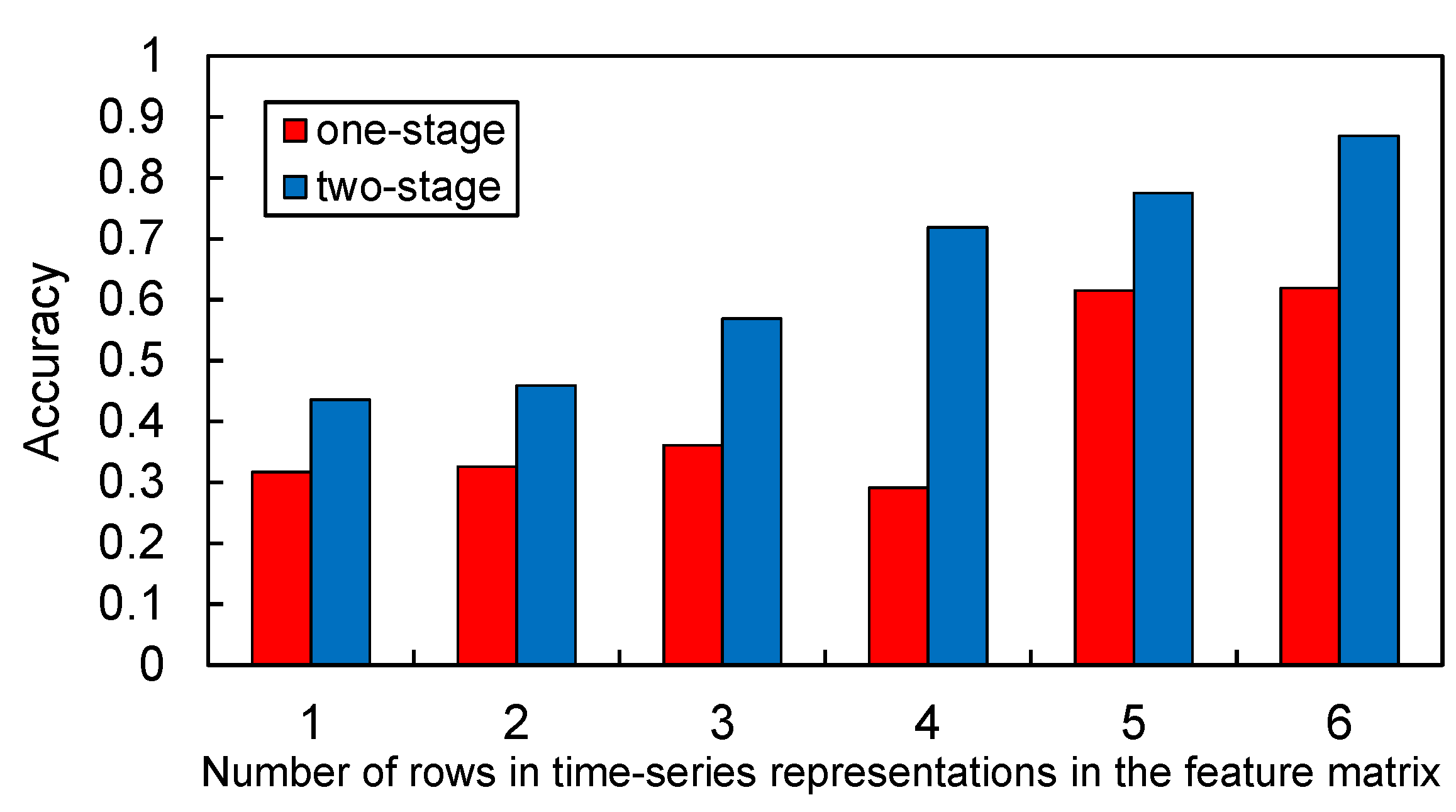
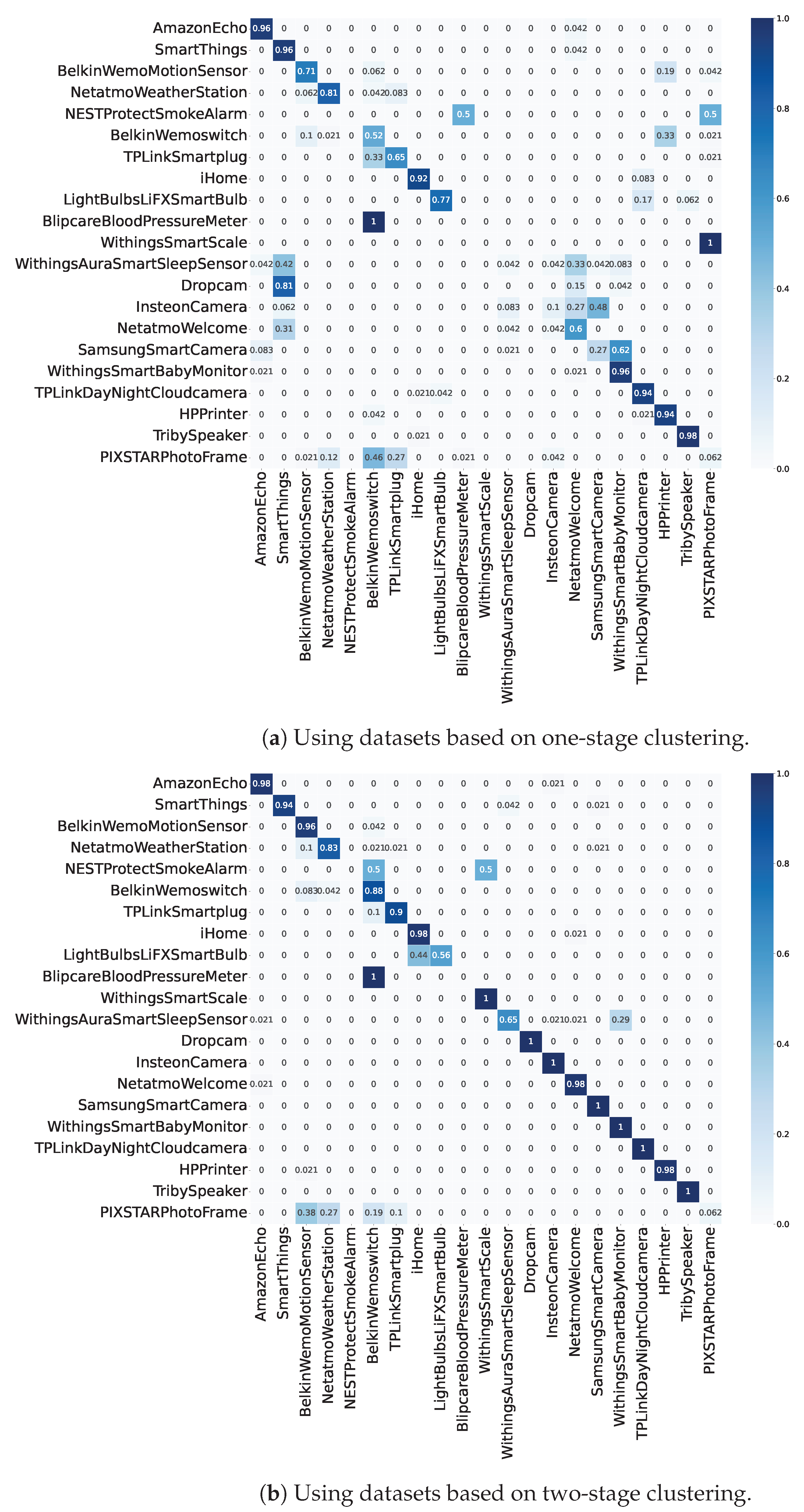
• We implemented an IoT device identification model with a long short-term memory (LSTM) network based on time series representations as the dataset. Using the proposed device identification model based on two-stage clustering, the accuracy with respect to identifying 21 IoT devices was 86.9%. The proposed method provides greater precision for both overall and for each IoT device identification than conventional single-stage centralized clustering. Moreover, by comparing the accuracies of six different time series representations as datasets, we demonstrated the effectiveness of analyzing IoT traffic over multiple time intervals.

The rest of this paper is organized as follows. Section 2 presents related studies on IoT device identification and introduces two-stage clustering [15,16], which is the basic concept of this paper. Section 3 presents an IoT traffic analysis method based on two-stage clustering. Section 4 presents and evaluates the analytical results of the two-stage clustering in comparison with those of one-stage clustering, which is similar to conventional methods. Section 5 proposes an IoT device identification method based on the analytical results obtained using two-stage clustering and evaluates the proposed method on indices of classification accuracy and efficiency. Finally, we assessed the effectiveness of distributed traffic analysis of IoT traffic using two-stage clustering. Section 6 presents the conclusions of the study and discusses future perspectives.

2. Related Work

2.1. IoT Device Identification Methods

Several identification methods of IoT devices have been proposed. Takasaki et al. proposed an IoT device identification method based on two-stage traffic analysis [6]. In the first step, this method extracts domain names from domain name system packets that IoT devices send regularly and estimates the manufacturers of the connected devices based on the domain names of the destination servers. Moreover, the method classifies devices into three categories, IoT devices, non-IoT devices, and routers, using supervised machine learning. By capturing all packets sent from each device in 10 min, the number of packets, total and average data sizes, the number of protocol types, and the number of destination addresses were extracted from the packets and used as feature values in the first-stage analysis. In the first step, the method classified connected devices into three categories with over 94% accuracy. The second step attempts to classify the functional categories of devices identified as IoT devices in the first step by analyzing traffic waveforms that represent the time variation of the transmitted packets. This method analyzed a set of 6000 packets collected from each IoT device every 100 milliseconds for 10 min as feature values using deep learning, a LSTM network [17], and a convolutional neural network. The accuracy of identifying the seven functional categories of the IoT devices was 83.7%. However, the accuracy of identifying reactive devices that operate in response to the actions of users and sensors, such as light bulbs, healthcare devices, and air quality sensors, was low.

Koike et al. proposed a method for identifying the called functions of IoT devices using the characteristic time variability of their generated traffic to visualize their operating status [7]. This method collects traffic data using specific functions on a smart speaker. Since the time variability of the communication traffic is discriminative for each function, 30 consecutive packets were set as one window. From each window, the average, variance, and standard deviation of the packet size, excluding the error packets from each transmission protocol, were extracted as feature values. In these experiments, 10 functions known as Amazon Echo Spots were estimated using a random forest. The results indicated that the classification accuracy of the ten functions was only 56.1%. The authors of this paper attribute the low accuracy to the labeling of even a no-communication period between function calls as part of each function and the definition of the window size. This method can automatically monitor the operation status of IoT devices, but the identification target is limited to one smart speaker.

Koike et al. proposed an improved version of this method [8]. This version uses two categories of features extracted from traffic data of functions called on three smart speakers: Amazon Echo Spot, Amazon Echo Dot, and Amazon Echo Flex. In the first category, the features extracted from each individual packet, such as the transport protocol, port number, and source and destination addresses, were used. In the second category, the features of each window consisting of 30 consecutive packets were used, as was done in [7]. However, they were extended to the average, variance, standard deviation, maximum, minimum, and difference between the maximum and minimum packet sizes. Random forests was employed as a machine learning algorithm based on comparisons of the identification accuracy of different supervised learning algorithms: random forests, extreme gradient boosting (XGBoost) [18], light gradient boosting machine (LightGBM) [19], and CatBoost [20]. In addition, regarding the treatment of the no-communication period, which was a factor contributing to low accuracy in the previous method when a function was not called before the first call or between calls, this method extracts idle time from the traffic data as a separate function. The experimental results demonstrated that the method could identify eleven called functions with an accuracy of 76.1% for the Amazon Echo Spot, nine functions with an accuracy of 89.8% for the Amazon Echo Dot, and had an accuracy of 85.2% for the Amazon Echo Flex. Moreover, a device identification method for the three types of Amazon Echo was implemented with an accuracy of 99.1%. This method can automatically and more precisely monitor how IoT devices operate than the previous method [7]. Nevertheless, the target is still limited to smart speakers only.

Hattori et al. proposed a method to estimate the execution functions on several types of IoT devices [9], which is also an extended version of the previous two methods. To examine the possibility of analyzing which functions of an IoT device have been executed, they used eight IoT devices from four categories: two smart cameras, two smart remote controllers, two smart speakers, and two smart plugs. The devices were connected to an edge router, where traffic data were collected during the execution of each function 10 s before and after execution. From the collected traffic data, the number and size of sending, receiving, TCP, and UDP packets, as well as the number of source and destination IP addresses in time windows of 0.5, 1, and 1.5 s were extracted. The mean, maximum, variance, and standard deviation values of the 30 extracted items were computed and evaluated based on the importance of the features calculated using random forests. Thereafter, the method selected and used 28 important features from 120 features as feature values and identified the function of the IoT device executed using random forests. The accuracy of detecting eight functions was 73%, and the accuracy of detecting 16 combinations of eight executed functions and two IoT devices in each device category was 91%. This method enables the automatic understanding of the behavior of not only smart speakers but also a wide variety of IoT devices.

Ammar et al. proposed an autonomous IoT device identification prototype [10], thereby outlining a methodology for an IoT device identification assistant and its architecture. The objective was to identify the types of devices that were newly connected to the home gateway to help end users better manage their devices and obtain more services from them. In feature selection, the first set of features was extracted from the flow characteristics of packet size, the interarrival time of flows, flow size, and protocol. In addition, the second set of features was extracted from the device description inspected from the packet payloads: the manufacturer name from the MAC address and the device name from the DHCP information. This method identified 28 IoT devices with an average accuracy of 98% using a decision tree. This method was considered for architectures designed to operate in smart home environments. However, all processing related to device identification was performed on a server, and the identification results were obtained on the web browser. This poses a problem in terms of user privacy protection.

Nguyen-An et al. proposed a method for visualizing IoT traffic characteristics and identifying IoT devices based on the average information content, which is known as information entropy [11]. This method analyzed IoT traffic properties by calculating the information entropy of the traffic parameters: the number of source and destination IP addresses, the number of source and destination ports, packet sizes, and the total amount of data for source IP addresses observed in five minutes. Subsequently, this method visualized them using behavior-shaped graphs. Moreover, an IoT device identification method based on the information entropy of IoT traffic features was implemented, and IoT devices were successfully identified with 94% accuracy. This method uses entropy to achieve time series feature extraction in IoT device communication. However, focusing on entropy in only a certain time interval could lead to inadequate feature extraction for some IoT devices.

Okui et al. proposed an identification of IoT device models in the home domain using IP flow information export (IPFIX) records [12]. The aim of this method based on IPFIX, which is a standard for flow information, is to reduce data volume for communication costs. In this method, IoT traffic captured on a gateway router was converted to IPFIX information, and the converted data were sent to the device identification server. Then, feature extraction from the IPFIX records and training of an identification model using LightGBM were operated on the server. As a result, this method identified 25 IoT devices with 98.48% precision. Moreover, using IPFIX records reduced the data volume to approximately 11% compared to traffic data. On the other hand, since all procedures for the IoT device identification were performed on a single server, there are concerns about the concentrated load.

Trad et al. proposed a method to mitigate frequent retraining for IoT device identification models [13,14]. A Siamese neural network (SNN) was trained to generate embeddings corresponding to the similarities of feature values. In this method, a database of embedding vectors corresponding to IoT traffic was created using an SNN. In the identification, 95 feature values extracted from IoT traffic were input to the identification model using an SNN, and an embedding vector was output. Then, the closest embedding to the output vector was searched from the database, and the input traffic was classified according to the IoT device corresponding to the retrieved embedding. When a new device was added, this IoT traffic was also input to the identification model using an SNN, and an embedding corresponding to the device was generated. And then, this embedding was added to the database. Therefore, the database was extended to include the new device type, and the model could recognize the new device without the updating. Based on the results in [14], this method yielded an 85.8% F-measure even when 28 unknown IoT device data were added after training. However, this method also processed traffic data at once, whereas all traffic data should be shared with the cloud servers in the real environments.

2.2. Considerations Regarding IoT Device Identification in Smart Home Environments

As mentioned previously, several IoT device identification methods based on traffic analysis with machine learning have been proposed. They automatically identify and understand IoT devices using traffic data. However, no consideration has been given to the implementation of these methods in a smart home environment.

IoT device identification in smart home environments involves three considerations. The first is the need to update identification models. This is because it is unlikely that IoT devices, once installed, will be used indefinitely in smart home environments. As new devices are installed and older devices are removed, frequent updating of the identification model and periodic training for model updating are essential to achieve proper management in response to the replacement of IoT devices installed in smart homes. However, conventional methods implement IoT device identification with only one-time learning and do not consider the computational and communication loads associated with model updating.

The second problem is how to process the traffic data. Analyzing a large amount of traffic data simultaneously in one place can cause a heavy load on the memory and CPU, as well as interfere with the analysis. With the growing use of IoT devices, the processing of a larger amount of collected IoT traffic is required. Although collecting and analyzing traffic data on a cloud server is one solution, this approach requires sending traffic data captured in smart homes to the cloud server every time the identification model is trained, which is unsuitable from the perspective of communication cost. Additionally, since IoT traffic contains a large amount of user information, uploading all the traffic data to the cloud server could lead to the leakage of user privacy. In addition, since the frequency of device usage and the amount of communication data vary by IoT device, biases potentially exist in the IoT traffic. The biases increase in proportion to the amount of traffic data, which potentially has a negative influence on traffic analysis. Therefore, it is necessary to consider how to process significant amounts of traffic data appropriately when implementing this method in smart home environments. However, conventional methods typically process traffic data simultaneously.

The third consideration is the target range for IoT device identification. Specific IoT devices in smart homes can be identified simply using static information such as IP and MAC addresses obtained from traffic data. From the perspective of security in smart homes, however, it is important to not only determine whether the appropriate IoT devices are connected but also to identify and grasp whether they are operating properly. Conventional methods analyze IoT traffic based on the communication properties, such as the number of destination IP addresses, protocol types, and the total amount of data. However, they only focus on the features extracted from traffic data for a fixed interval, and they accordingly ignore that each IoT device has different communication and operation cycles. Thus, they overlook the behavior of IoT devices because they cannot extract features from some IoT traffic owing to variations in the communication periods or behavior.

3. IoT Traffic Analysis with Two-Stage Clustering

Based on the current situation of IoT device security and the issues with conventional methods, we propose a method for analyzing IoT traffic and identifying IoT devices based on the time series properties of IoT traffic for operation in smart home environments. The first aim of this paper is to ensure security in smart home environments. The proposed method only uses the communication traffic of IoT devices and automatically identifies what kinds of IoT devices are used. By checking the identification results, users can obtain information about what kind of devices are operating. Furthermore, the proposed method uses two-stage clustering [15,16] to avoid user privacy leakage caused by uploading IoT traffic itself to a cloud server. The second aim is to distribute the computational costs in traffic analysis. The proposed method operates in two locations: gateway routers installed in smart homes and a cloud server. Note that it is not necessary to implement the proposed method on IoT devices. The proposed method comprises two phases: an IoT traffic analysis phase with two-stage clustering and an IoT device identification phase based on time series representations. In this section, we describe the first phase of the proposed method.

3.1. Two-Stage Clustering

In the proposed method, we focus on two-stage clustering, which is the basis of the proposed method. Two-stage clustering is a traffic analysis method that aims to obtain dynamic changes in P2PTV traffic as proposed in [15,16]. As a preliminary preparation, the traffic data when viewing each P2PTV video content were divided into predetermined unit time lengths. In the first-stage clustering, the set of divided traffic data was clustered using k-means clustering for each P2PTV content. The representative values were extracted from each cluster obtained from the first clustering. Representative values corresponding to all the first-stage clusters were gathered and clustered again using k-means clustering. These clustering steps possibly equalize the biases of the occurrence frequency of traffic patterns, because every cluster is described as one value, regardless of the cluster size. Hence, two-stage clustering extracts traffic patterns irrespective of the occurrence frequency. In [15], the patterns obtained by two-stage clustering were used to illustrate the transition characteristics of P2PTV traffic. In [16], comparisons of one- and two-stage clustering confirmed the effectiveness of two-stage clustering in P2PTV traffic analysis.

There are three reasons for applying the two-stage clustering in the proposed method. First, the two-stage processing can realize load distribution, which is one of the considerations when assuming implementation in actual environments. For instance, the first clustering step is performed at a gateway in each smart home, and the clustering results are subsequently transferred to a cloud server and clustered in the second stage. Thus, the entire clustering process is distributed in the network. Second, the concept that every cluster is described as one value regardless of the cluster size can reduce the impact on IoT traffic analysis from the biases of traffic data, which is similar to P2PTV traffic analysis. Moreover, this representation mechanism can reduce communication traffic when combined with the distributed implementation described above. Only representative values of the clusters are transferred from each smart home to a cloud server. Third, the objective of two-stage clustering [15,16] to obtain dynamic changes in P2PTV traffic coincides with the need to determine whether an IoT device functions normally or appropriately, thereby addressing the concerns raised in the context of conventional methods. This is because two-stage clustering primarily divides traffic data into a series of data pieces and thus realizes time series data analysis. Therefore, we decided to use a two-stage clustering in the proposed method.

3.2. Procedure of the Proposed Method

Figure 1 shows an overview of the IoT traffic analysis using the proposed method. This method analyzes IoT traffic in two steps at two locations: gateway routers installed in smart homes for the first step analysis and a cloud server for the second step analysis. In the first step, the IoT traffic data are preliminarily divided into data pieces per unit of time. From the divided traffic data pieces, feature values are extracted and subsequently clustered for each IoT device at the gateway router in each smart home. This is the first clustering. Next, representative values are extracted from each cluster generated by the first clustering and treated as the cluster feature. In this paper, a representative vector composed of the averages of all the feature values in each cluster was used. Thereafter, the cluster features were sent from each gateway router to the cloud server. Thus, by avoiding sending raw traffic data and feature values of all traffic data pieces, the communication load between the gateway routers and cloud server is reduced. In the second step, the cloud server executes another clustering process using all the cluster features for all the IoT devices gathered from the gateway routers: This is the second clustering. The clusters extracted by the second clustering on the cloud server are defined as the unit traffic. A series of unit traffic can represent a set of elemental patterns generated by IoT devices.

The unit traffic patterns resulting from the second clustering are sent back from the cloud server to the gateway routers. The gateway routers compare the results of the first and second clustering and thereafter assign appropriate unit traffic numbers to all the original divided data pieces. Finally, the IoT traffic is represented by a series of unit traffic numbers as a time series representation. This process is illustrated in Figure 2.

Here, we consider the treatment of traffic data when an IoT device has no communication in terms of the unit of time. Some IoT devices tend to have long intervals between communication periods because of periodic sensing operations or passive response behaviors, particularly in response to user requests. When the traffic data generated by such IoT devices are divided into a series of data pieces according to the value of the unit of time, a significant number of data pieces do not contain any communication information, which could affect the clustering results. However, a traffic data piece without any packet transmission can be clearly and easily recognized at the stage of capturing the IoT traffic. Therefore, traffic data pieces without any communication were removed from the datasets for the first and second clusters. Meanwhile, since the no-communication state is still important for characterizing IoT traffic, we defined the traffic data piece without any communication as zero traffic, which is one of the units of traffic patterns.

3.3. Experimental Conditions

In these experiments, k-means clustering [21] was used as the clustering method. The k-means clustering algorithm is a nonhierarchical clustering algorithm in which the number of clusters must be specified in advance, and the samples are divided into a predetermined number of clusters. It has the advantages of high computing efficiency and generality regardless of the data size. However, it is necessary to determine the number of clusters. Furthermore, the results of k-means clustering depend on the initial values of the cluster centroids, which are generally randomly determined. The procedure for k-means clustering is as follows [21]:

• Set k centroids of clusters randomly (initialization). The number of clusters, k, must be determined in advance.
• Traverse all data points and calculate the distances between all centroids and data points. Clusters are formed based on the minimum distance from the centroids.
• The average value of the data in each cluster is calculated as the new cluster centroid.
• The second and third steps are repeated until the centroids stop moving; that is, the centroids no longer change their positions and become static.

In k-means clustering, the number of clusters must be determined in advance, and the appropriateness of this value should be verified. Therefore, in this paper, we used silhouette analysis [22] as a metric to evaluate the validity of the number of clusters. Silhouette analysis is based on the silhouette coefficient in which a data point $x_i$ classified into cluster $C_{in}$ is calculated, which is defined as follows:

• Calculate the average distance $a_i$ between $x_i$ and the other data points within $C_{in}$ by using the following equation:

  $$\begin{array}{c}\hfill a_i=\frac{1}{|C_{in}|-1}\sum _{x_j\in C_{in}}\parallel x_i-x_j\parallel .\end{array}$$

  (1)
• Calculate the average distance $b_i$ between $x_i$ and all data points assigned to $C_{near}$, which is the cluster nearest to $x_i$ other than $C_{in}$, using the following equation:

  $$\begin{array}{c}\hfill b_i=\frac{1}{|C_{near}|}\sum _{x_j\in C_{near}}\parallel x_i-x_j\parallel .\end{array}$$

  (2)
• Calculate the silhouette coefficient $s_i$ using $a_i$ and $b_i$ through the following equation:

  $$\begin{array}{c}\hfill s_i=\frac{b_i-a_i}{max(a_i,b_i)}.\end{array}$$

  (3)

As expressed in Equation (3), the range of $s_i$ is $[-1,1]$. The clustering performance was found to be the best when $s_i=1$. Meanwhile, we found that data point $x_i$ may not be correctly clustered if $s_i<0$. After calculating the silhouette coefficient for all data points using the aforementioned steps, the clustering performance was measured using the average value.

For feature values, we selected 10 indices consisting of both sending and receiving features of the following five factors: average throughput (abbreviated as ave, particularly in figures; the same applies hereafter), maximum throughput (max), the variation coefficient of throughput (CV), the number of IP addresses (IP), and the number of ports (port) in units of time. The units of time were set at 30, 60, 120, 300, 600, and 900 s. We used the dataset captured by Sivanathan et al. on 28 September and 4 October 2016 [23], which contains the traffic data of 21 IoT devices, as summarized in

Table 1. IoT devices and their categories in the dataset used in this paper [23]. The dataset consists of 21 IoT traffic datasets and six device categories: two smart speakers, three smart sensors, four smart plugs, three healthcare devices, six smart cameras, and three smart gadgets.

Device Category	IoT Device
Smart speakers	Amazon Echo
	Smart Things
Smart sensors	Belkin Wemo Motion Sensor
	Netatmo Weather Station
	NEST Protect Smoke Alarm
Smart plugs	Belkin Wemo Switch
	TP-Link Smart Plug
	iHome
	Light Bulbs LiFX Smart Bulb
Healthcare devices	Blipcare Blood Pressure Meter
	Withings Smart Scale
	Withings Aura Smart Sleep Sensor
Smart cameras	Dropcam
	Insteon Camera
	Netatmo Welcome
	Samsung Smart Camera
	Withings Smart Baby Monitor
	TP-Link Day Night Cloud Camera
Smart gadgets	HP Printer
	Triby Speaker
	Pix-Star Photo Frame

.

4. Analytical Results

In Section 3, we explain the IoT traffic analysis of the proposed method, thereby assuming its implementation in a smart home environment. Before implementation, we must confirm the effectiveness of the IoT traffic analysis using two-stage clustering. Therefore, in this paper, we implemented one-stage clustering on a single computer and verified whether IoT traffic analysis using two-stage clustering functioned properly based on the analytical results.

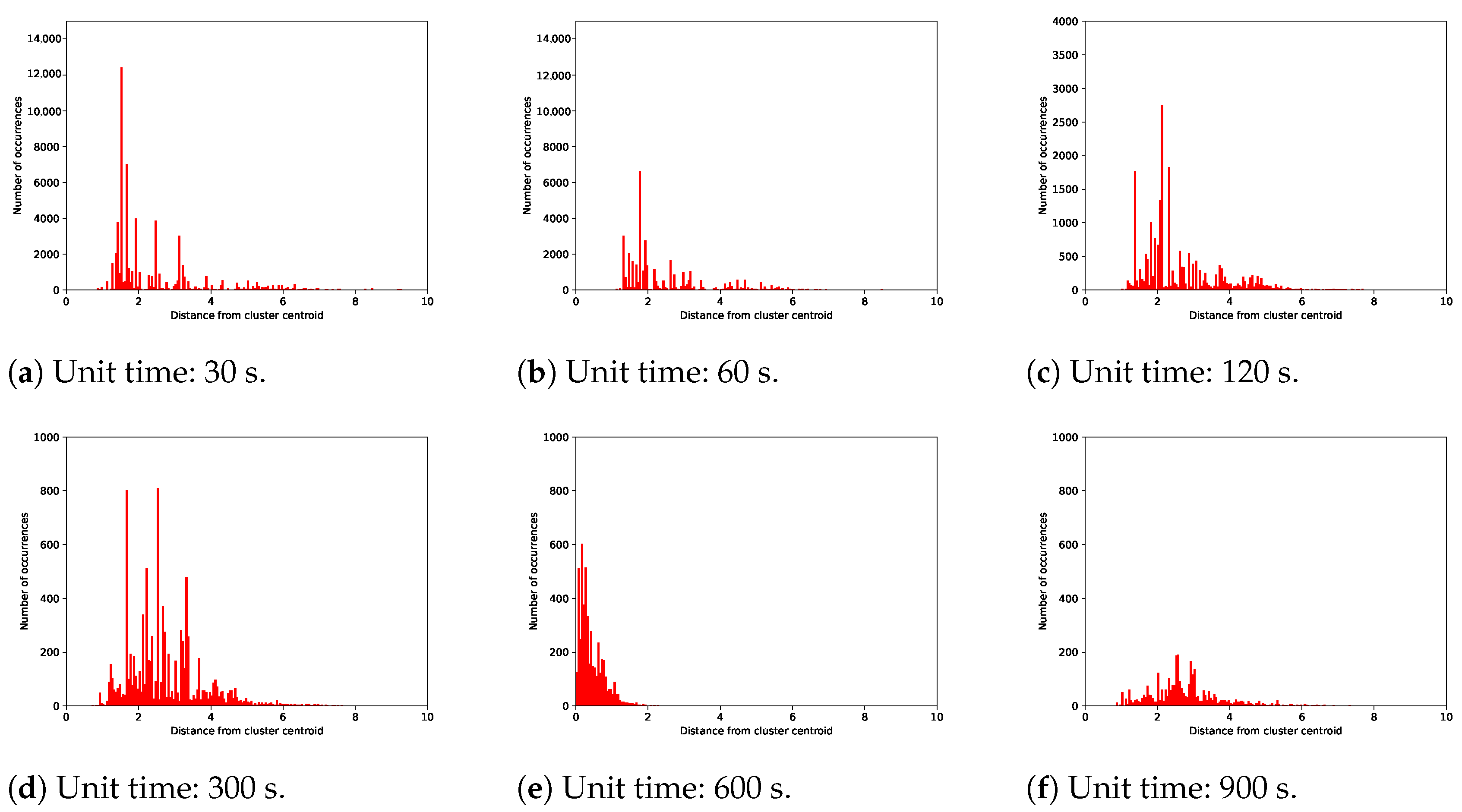
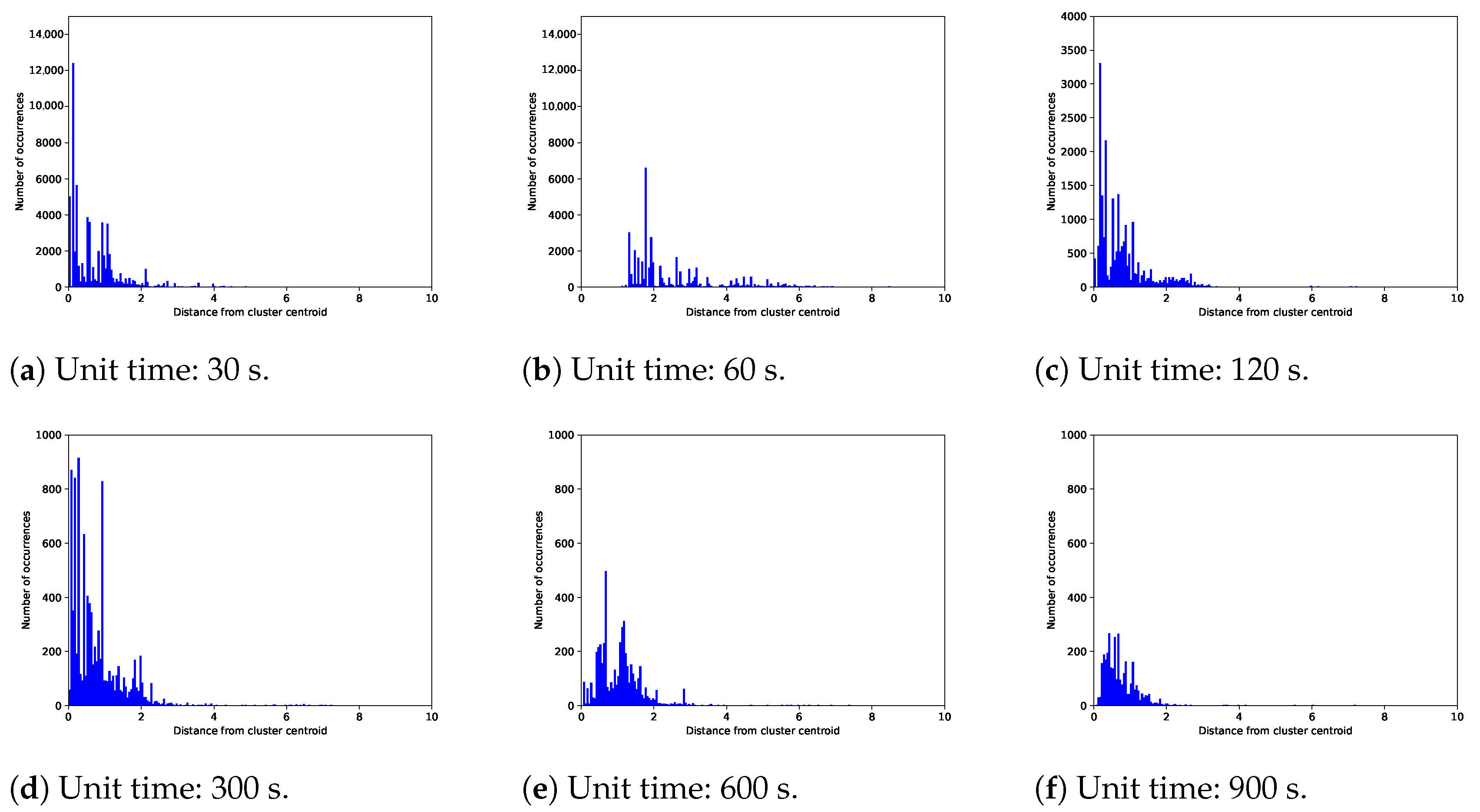
4.1. One-Stage Clustering as a Comparison Target

To evaluate the two-stage clustering, we used one-stage clustering for comparison purposes. Figure 3 and Figure 4 present an overview of the one-stage clustering method for IoT traffic analysis. First, the IoT traffic data are divided into data pieces per unit of time. Feature values are extracted from the divided data in each gateway router following the same steps as the two-stage clustering explained in Section 3. Second, unlike the proposed method with two-stage clustering, the feature values of all the divided data pieces are sent to the cloud server without clustering at the gateway routers. These values are clustered simultaneously on the cloud server. The clusters generated in this one-stage clustering are treated as unit traffic patterns, which is similar to the clusters extracted in the second clustering using the proposed method. Zero traffic, which is a type of unit traffic pattern without any communication, is also used in one-stage clustering. The unit traffic information, which consists of the feature values of the original divided data pieces and their assigned unit traffic numbers, is sent to the gateway routers. In this paper, we implemented a one-stage clustering method on a single computer as a conventional method for comparison.

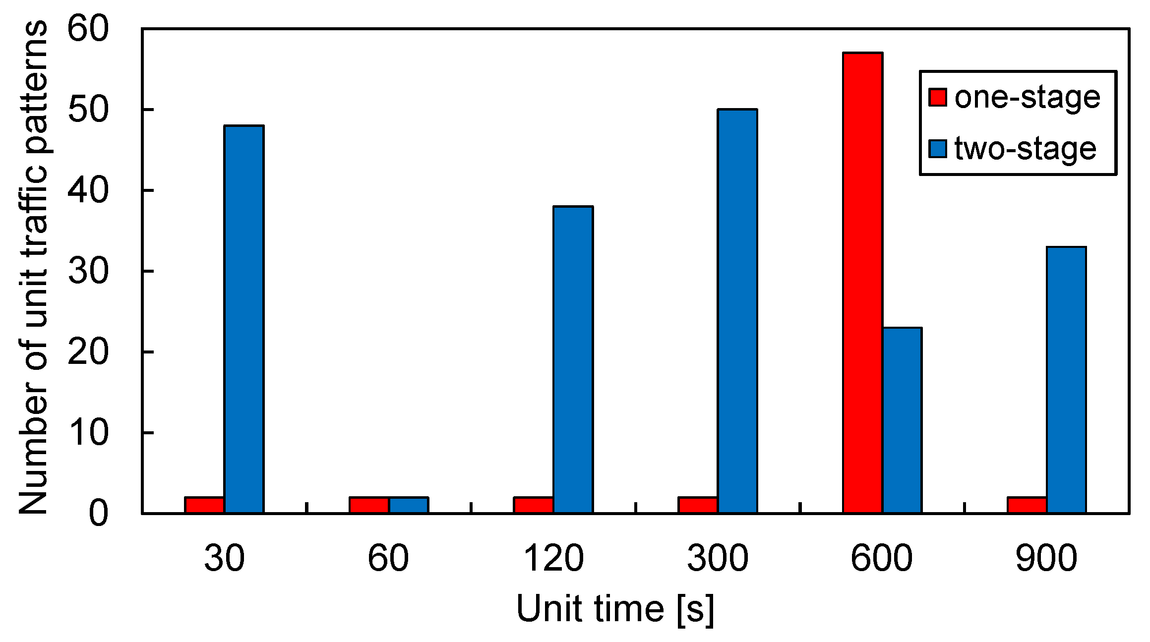
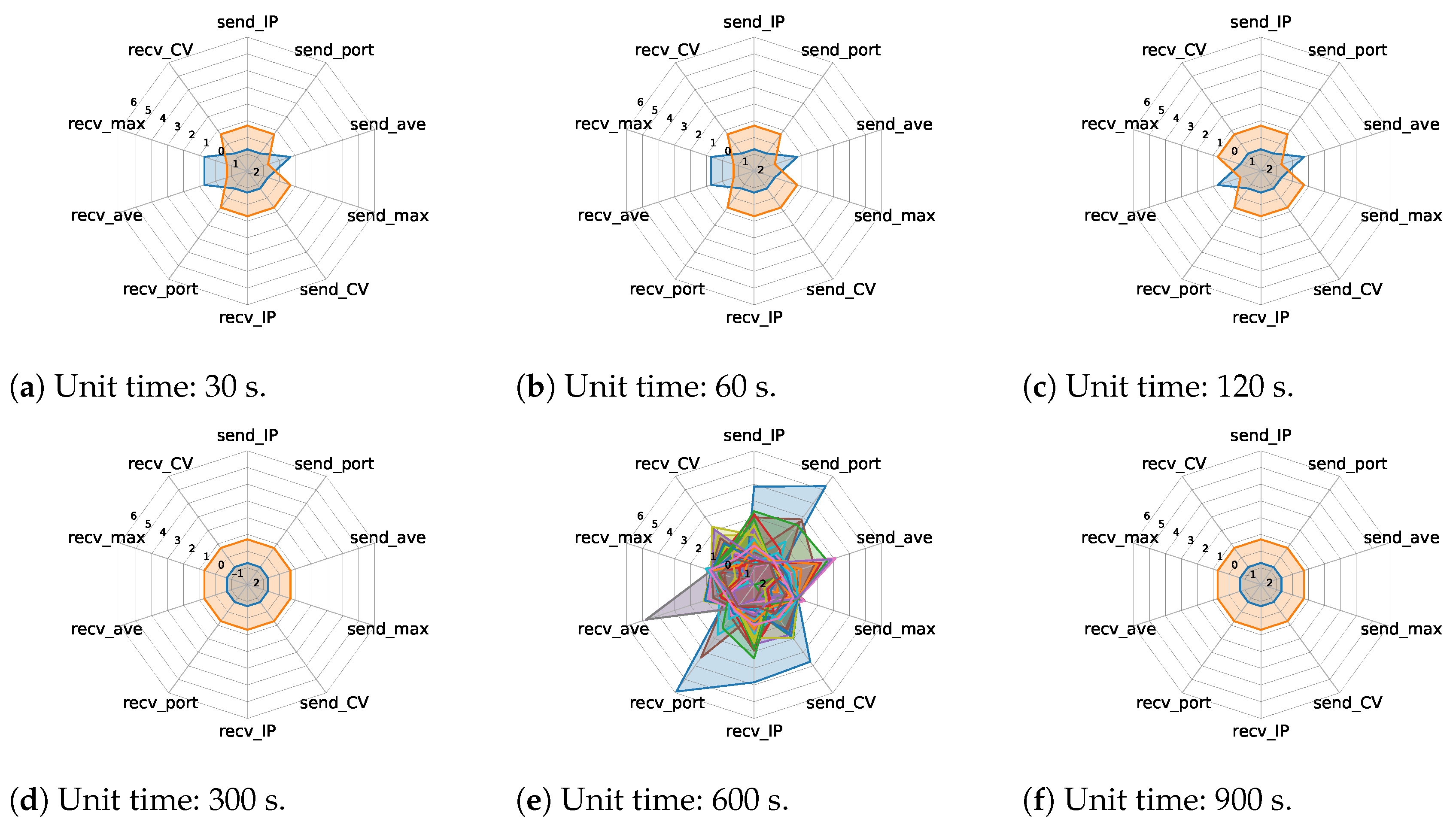
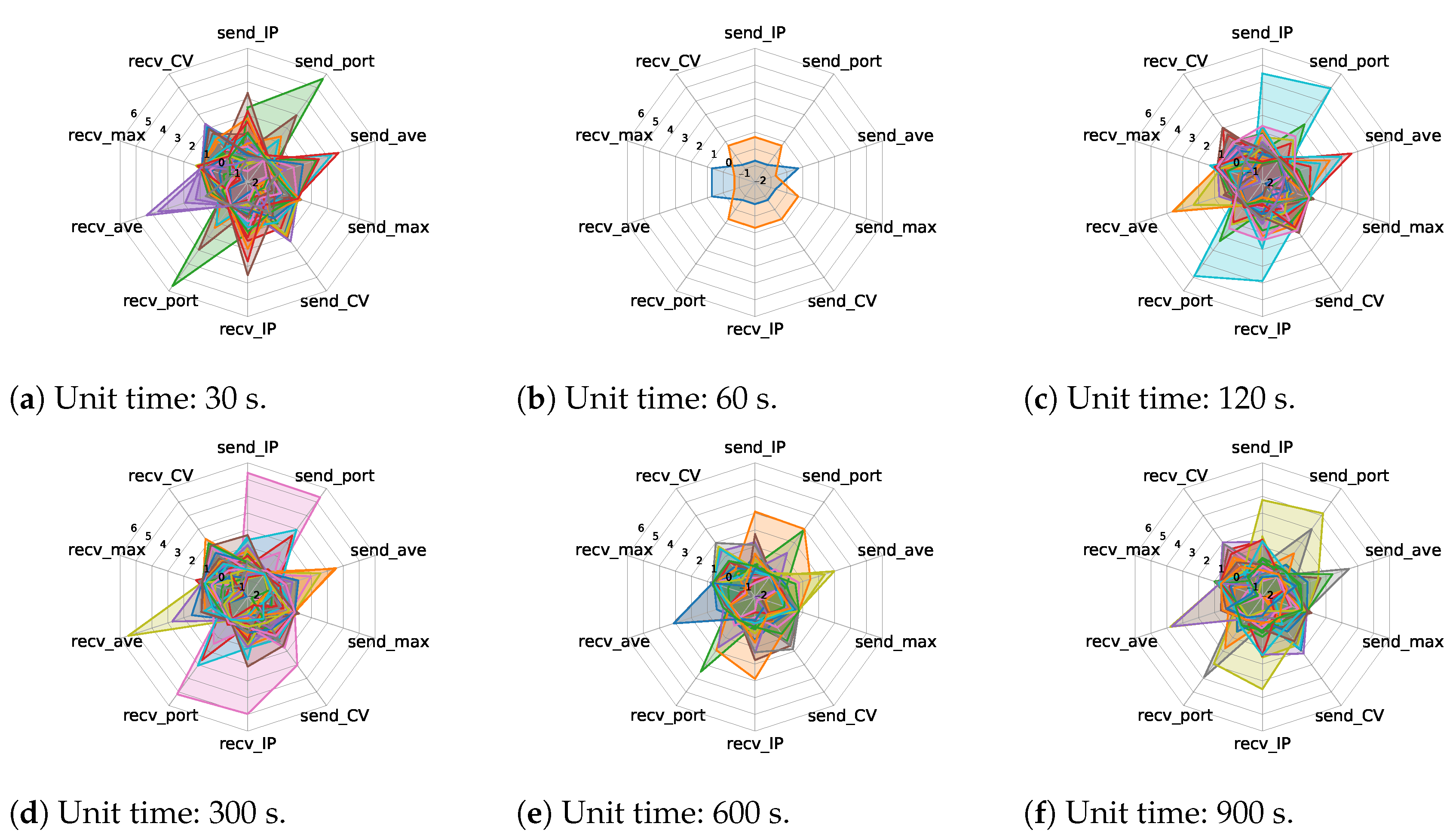
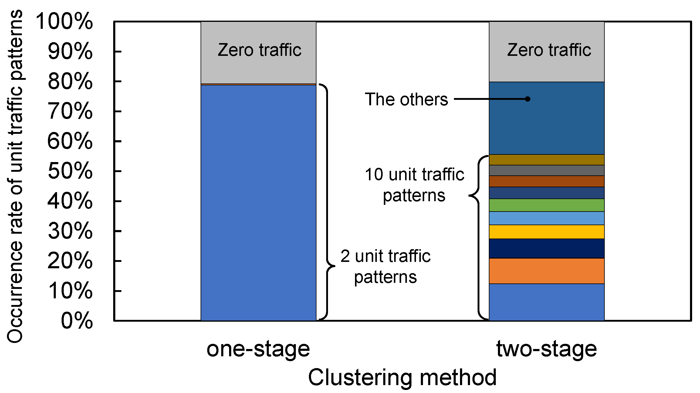
4.2. Unit Traffic Patterns Extracted by One/Two-Stage Clustering

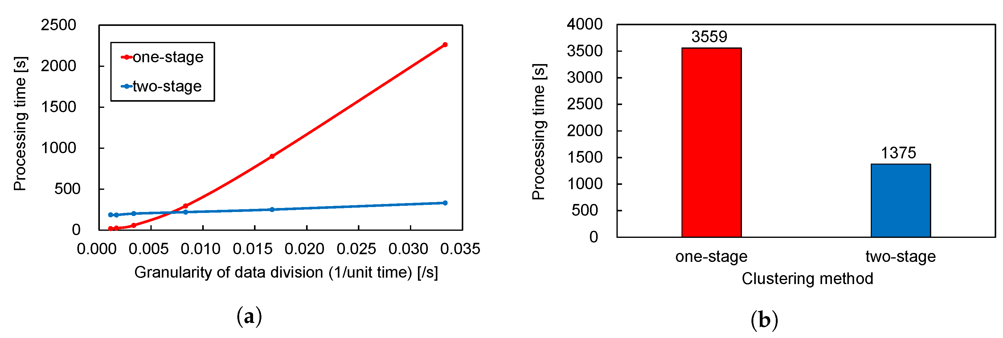
Figure 5 shows the number of unit traffic patterns extracted using one- and two-stage clustering in red and blue, respectively. A larger number of unit traffic patterns was extracted by two-stage clustering than by one-stage clustering, except when the unit of time was set at 600 s. In addition, the number of unit traffic patterns extracted using two-stage clustering varied significantly depending on the length of the unit time.

Figure 6 and Figure 7 show the cluster features of the unit traffic patterns extracted using one- and two-stage clustering using radar charts, respectively. Comparing these two figures, although some types of characteristic shapes can be extracted, there were several overlapping parts in the radar charts when the two-stage clustering was used. Since the overlap of shapes in the radar chart indicates the similarity of features, two-stage clustering tends to redundantly extract unit traffic patterns with similar features. In contrast, while it could be considered that the one-stage clustering can extract the minimum number of unit traffic patterns necessary to express the features of IoT traffic in several cases, these patterns may appear overly simplistic, since all 10 feature values are solely classified as large or small.

Figure 8 and Figure 9 show the frequency distributions of the Euclidean distances of the feature values of each divided traffic data piece (i.e., representative vector) from the cluster features of the unit traffic corresponding to that data piece (i.e., cluster centroid) for one- and two-stage clustering, respectively. These two figures show that the spread of the distance distributions for two-stage clustering was narrower than that for one-stage clustering.

Table 2. Statistical data regarding the distances of the feature values of divided traffic data pieces from the cluster features of the corresponding unit traffic pattern. The left column represents the statistical metrics when the unit of time was 120 s, and the right column shows the same metrics at all settings of the units of time. The proposed two-stage clustering method can classify divided traffic data pieces with more similar characteristics.

Clustering	Distance from Cluster Feature (Unit of Time: 120 s)				Distance between Cluster Features (All Settings of Units of Time)
	Ave	Max	Min	Var	Ave	Max	Min	Var
One-stage	2.70	31.9	0.84	1.76	2.93	9.99	0.55	2.41
Two-stage	0.82	18.5	0.00	0.81	3.84	11.4	0.15	2.09

lists the statistical data of the Euclidean distances shown in Figure 8 and Figure 9. The left column of Table 2 presents the four statistical metrics: the average, maximum, minimum, and variance in distances from the corresponding cluster features when the unit time was 120 s. For two-stage clustering, all the metrics were significantly smaller than those for one-stage clustering. Thus, two-stage clustering can be used to classify segmented traffic data with similar characteristics. The right column of Table 2 presents the metrics at all the settings of the unit of time. The average and maximum distances were greater for the two-stage clustering. Although the minimum distance of two-stage clustering was less than that of one-stage clustering, this does not indicate poor clustering performance when the number of unit traffic patterns extracted using one- and two-stage clustering is considered. According to the results regarding the Euclidean distances of the traffic data pieces from the corresponding cluster centroids, two-stage clustering can extract unit traffic patterns with different characteristics and is less likely to misclassify traffic patterns with different features into the same unit traffic pattern.

4.3. Execution Time

As mentioned in Section 2, it is necessary to evaluate whether the proposed method can cope well with model updating and processing significant amounts of traffic data, particularly regarding the computational load. Therefore, we measured the processing time using the time module in Python [24] when one- and two-stage clustering executed all the processes mentioned in Section 4.1 and Section 3.2, respectively. The processing time includes dividing each traffic data into data pieces to extract unit traffic patterns for each unit of time for the 21 IoT traffic datasets.

Figure 10a shows the processing time transition of one- and two-stage clustering with respect to the number of divided data pieces, thereby representing the granularity of the data division, which can be proportionally expressed as the reciprocal of the unit of time. When the granularity was less than 0.005, that is, when the unit of time was 300 s or larger, one-stage clustering required a shorter time than two-stage clustering. However, the processing time of the one-stage clustering rapidly increased as the granularity exceeded 0.005, whereas that of the two-stage clustering remained almost flat. From this perspective, the proposed two-stage clustering method has the advantage of increasing the amount of IoT traffic data that can be processed.

In this paper, we not only performed clustering but also created the combined time series representation of IoT traffic data using six values of units of time to grasp the more specific time variability properties of IoT traffic. The total time to perform clustering six times while varying the unit of time from 30 to 900 s is thus more important. Figure 10b shows the total time spent when executing the one- and two-stage clustering methods. The two-stage clustering took approximately 61% less time than the one-stage clustering. Therefore, even in terms of the total processing time, the proposed two-stage clustering outperformed the one-stage clustering.

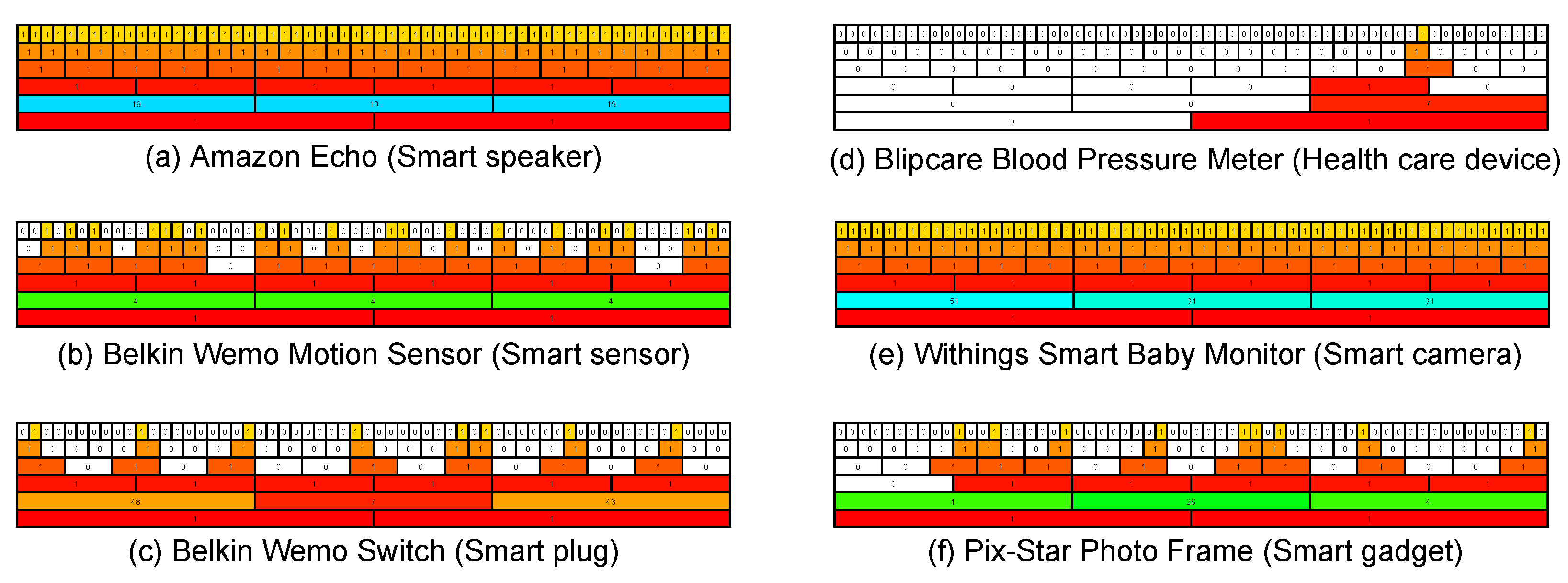
4.4. Time Series Representation

The set of unit traffic patterns extracted by the clustering methods was used to convert the IoT traffic into a time series representation. In this paper, we set the following two rules to express the time series features of IoT traffic. The first is the scale of the unit traffic pattern. In Section 4.2, six sets of unit traffic patterns were obtained when the unit time was set at 30, 60, 120, 300, 600, and 900 s. Therefore, we leveraged all sets of unit traffic patterns as displayed in two dimensions: the vertical direction represents the set of the unit of time; thus, each representation has six rows from 30 to 900 s. The horizontal direction represents the passage of time from left to right; the width is set at 1800 s as the least common multiple (LCM) of the six values of units of time. The sequence of numbers in each row indicates the time series unit traffic numbers. Thus, the width of two 900-second units (=1800 s) is equal to that of three 600-second units, six 300-second units, 15,120-second units, and so on. The second rule concerns the color of the unit traffic pattern. In this paper, the colors of all unit traffic patterns extracted at all sets of units of time were selected according to the Euclidean distances of their 10 dimensional features from unit traffic patterns; No. 1 was extracted when the unit of time was 900 s, which is the basis of the unit traffic patterns. The color of the basis of the unit traffic patterns was set to red, and the other traffic units were colored yellow, green, blue, or purple, depending on the distance from the basis. Therefore, the unit traffic pattern close to the feature space (i.e., with similar features) has a similar color. However, since color is determined only by the Euclidean distance in the 10 dimensional feature space, unit traffic patterns with different features may exhibit similar colors. Zero traffic is indicated in white. Note that the color and number of traffic units were assigned without any relation to the features of the unit traffic.

Figure 11 and Figure 12 show the time series representations of six IoT devices based on one- and two-stage clustering: the Amazon Echo (smart speaker), Belkin Wemo Motion Sensor (smart sensor), Belkin Wemo Switch (smart plug), Blipcare Blood Pressure Meter (healthcare device), and Pix-Star Photo Frame (smart gadget), respectively. Since we defined zero traffic as one of the unit traffic patterns and colored it white, the time series representations based on both clustering methods could be described whenever each IoT device communicated. In Figure 11, the representations of all IoT devices obtained using one-stage clustering consist of the same unit traffic pattern and/or zero traffic except for the 600-second unit of time and thus do not represent how each IoT device communicates in each unit of time. These phenomena are derived from the fact that only two unit traffic patterns were extracted in several cases using one-stage clustering, as shown in Figure 7. In contrast, Figure 12 shows that the representations obtained using two-stage clustering exhibit various colors. Therefore, the representations based on two-stage clustering can better represent the differences in the communication traffic behavior of IoT devices.

Figure 13 shows the occurrence rate of the unit traffic patterns, including zero traffic, in the time series representations of the 21 IoT traffic datasets when the unit of time was set at 900 s. Although one-stage clustering extracts only two unit traffic patterns, the occurrence rate has a significant bias between them: more than 99% of the divided data pieces, except for zero traffic, exhibit the same unit traffic pattern. However, the time series representation extracted using two-stage clustering when the unit of time was set at 900 s comprises various unit traffic patterns with a certain proportion. Hence, time series representations based on two-stage clustering can represent the time series characteristics of each IoT traffic item in more detail than one-stage clustering.

4.5. Summary

In this section, we evaluate the proposed two-stage clustering method by comparing it with one-stage clustering in terms of the clustering performance, unit traffic patterns, and time series representations of the extracted unit traffic patterns. The comparison results indicate that the IoT traffic analysis with two-stage clustering can provide more detailed communication features for IoT devices. Moreover, we demonstrated that two-stage clustering can reduce the impact of an increase in traffic data volume on the processing load in clustering.

In this paper, we implemented the proposed two- and one-stage clustering methods on a single computer to analytically verify whether they function properly. However, when implementing the proposed method in real environments, data communication occurs between the gateway routers in smart home environments and the cloud server to exchange the feature values of the divided traffic data pieces and their cluster features. In the future, we will investigate the impact of communication in real network situations.

5. IoT Device Identification Based on Time Series Representations

In Section 3, the IoT traffic analysis phase of the proposed method was introduced. By analyzing the IoT traffic using two-stage clustering and transforming it into time series representations, we successfully extracted and visualized the time series features of IoT traffic. In this section, we propose an IoT device identification phase based on time series representations.

5.1. Procedure of IoT Device Identification

First, we describe the creation of a dataset for IoT device identification. Figure 14 shows an example of a representative feature matrix, which can be easily obtained from the time series representations shown in Figure 11 and Figure 12. Similar to these figures, the rows show the time series representations of IoT traffic when the units of time were 30, 60, 120, 300, 600, and 900 s from top to bottom. In addition, the horizontal direction from left to right represents the passage of time, whose width was set at 1800 s as the LCM of the six values of units of time. The width scale of every unit of time was unified to 1800 s. To use time series representations as a representative feature matrix for IoT device identification, the unit widths of the time series representations at every unit of time must be aligned. Therefore, the width of the time element in the feature matrix was set at 30 s, which is the greatest common divisor of the six values of units of time. The first row of the feature matrix consists of 60 continuous unit traffic numbers of independently divided data pieces extracted when the unit of time is 30 s. Similarly, the bottom row has two sets of continuous unit traffic patterns when the unit of time is 900 s; however, each is divided into 30 blocks with the 30-second time element and assigned the same unit traffic number. Thus, the matrix of the time series representations created using the aforementioned approach has $6\times 60$ elements and is treated as a set of feature values labeled for each IoT device. Zero matrices, which consisted of zero traffic only, were excluded from the dataset for IoT device identification.

To identify the IoT devices, this paper applied an LSTM network [17], which is a well-known time series analysis method. Adaptive moment estimation (Adam) [25], which is also popular in optimization methods in deep learning, was used as the optimization algorithm. For the processing flow of the device identification, a series of feature matrices created from the time series representations were input into the identification model using LSTM. Thereafter, the model predicted which IoT device the input dataset belonged to and output one data label corresponding to the device.

5.2. Experimental Conditions

In the experiments, two comparison targets were prepared to evaluate the effectiveness of the proposed method. First, we used the matrices based on the time series representations with one- and two-stage clustering as the datasets. Second, the $n\times 60$ ($n=\{1,2,\cdots ,6\}$) matrices obtained by extracting n rows from the top of the representation shown in Figure 14 were used as the input data. The second comparison evaluated whether analyzing IoT traffic with multiple values of units of time can reveal time variability in more detail.

For the parameters of the identification model, the number of LSTM layers and their hidden layers were set at 2 and 64, respectively. As the input traffic data, the same dataset [23] consisting of 21 types of IoT devices listed in Table 1 used for the IoT traffic analysis in Section 3 was used. For the training phase of the LSTM network, the traffic data captured on 28 September 2016 were used: 80% of them were randomly selected as the training dataset, and the remaining 20% were used as the validation dataset. For the evaluation phase of the trained model, traffic data captured on 4 October 2016 were used as the test dataset.

As indices for performance evaluation, we introduced four typical machine learning metrics: accuracy, recall, precision, and F-measure. As the recall, precision, and F-measure were obtained for each IoT device classification, we used their averages to evaluate the overall classification performance.

5.3. Results

Figure 15 shows the accuracy of the proposed IoT device identification method using six types of time series representations as the input data. IoT device classification was found to be more accurate when the time series representations had more types of time units. The obtained identification results can be attributed to the increase in the number of feature values included in each matrix. In addition, by training the identification model using input data with multiple values of time units, it can address differences in communication timing and cycles among IoT devices and thereafter extract the characteristics and differences in IoT traffic in more detail. This tendency was observed regardless of the clustering method used. Nevertheless, when the input data had the same format, the identification model with two-stage clustering always outperformed that with one-stage clustering.

Table 3. Performance outcomes of the identification models. Based on all four evaluation metrics, the identification model based on two-stage clustering clearly exhibits a better identification performance.

Clustering	Accuracy	Recall	Precision	F-Measure
One-stage	0.619	0.533	0.499	0.490
Two-stage	0.869	0.795	0.793	0.762

lists the performance outcomes of the identification models when using the datasets generated using the one- and two-stage clustering methods. Based on all four evaluation metrics, it is clear that the identification model using two-stage clustering exhibited a better identification performance than that using one-stage clustering. Figure 16 shows the confusion matrices of the 21 IoT device identifications. In terms of the identification accuracy per IoT device, the identification model using two-stage clustering also performed better than that using one-stage clustering. Specifically, the difference was particularly significant in the identification accuracies of the smart camera categories: Dropcam, Insteon Camera, Netatmo Welcome, and Samsung Smart Camera. Smart cameras typically maintain a continuous communication process by regularly uploading video data to the cloud. As mentioned in Section 4.2, one-stage clustering can only extract two unit traffic patterns, and the occurrence rate of one was greater than 99%. This means that the feature matrices can only recognize that the device always communicates and cannot distinguish traffic differences, such as throughput and the number of IP addresses and ports. Therefore, time series representations using one-stage clustering cannot adequately identify smart camera devices. Hence, as also shown in Figure 11 and Figure 12, we can conclude that two-stage clustering can more appropriately extract features that are important to describe IoT traffic, and the time series representations based on two-stage clustering can express not only whether but also whatever an IoT device communicates.

Table 4. Comparison of identification performance outcomes between the proposed method and the conventional methods [6,7,8,9,10,11,12,13,14].

Method	Data Processing	Accuracy	Recall	Precision	F-Measure
Proposed	Distributed	0.869	0.795	0.793	0.762
Takasaki et al. [6]	Centralized	0.837	-	-	-
Koike et al. [7]	Centralized	0.561	-	-	-
Koike et al. [8]	Centralized	0.898	-	-	-
Hattori et al. [9]	Centralized	0.910	-	-	-
Ammer et al. [10]	Centralized	0.980	-	-	-
Nguyen-An et al. [11]	Centralized	0.940	-	-	-
Okui et al. [12]	Centralized	-	-	0.985	-
Trad et al. [13,14]	Centralized	-	-	-	0.858

shows a comparison of the identification performance outcomes between the proposed method and the conventional methods [6,7,8,9,10,11,12,13,14]. Although it is difficult to strictly compare among them due to the lack of detailed data, the identification accuracy of the proposed method is higher than some of the conventional methods [6,7,8] but slightly lower than the others [9,10,11,12,13,14]. This could be because some traffic features were lost due to feature extraction by clustering. On the other hand, our method has an advantage of being able to be implemented in a distributed environment. We will try to improve the identification performance in the future.

6. Conclusions

In this paper, we proposed a method for IoT traffic analysis and device identification based on two-stage clustering in smart home environments and verified whether the proposed method functioned properly by comparing it with one-stage clustering. Consequently, IoT traffic analysis using two-stage clustering grasped the features of IoT traffic more specifically and appropriately with a shorter computation time. Moreover, IoT device identification using representative feature matrices based on two-stage clustering enabled the identification of 21 devices with an accuracy of 86.9%. Therefore, we observed that the distributed IoT traffic analysis and device identification based on two-stage clustering performed appropriately. On the other hand, compared to some conventional methods, the proposed method showed poor identification performance. This is because machine learning was used for both feature extraction and identification phases. However, the proposed method is intended not only to ensure security through the automatic identification, but also to perform load balancing and to protect user privacy. Therefore, in order to verify the overall effectiveness of the proposed method, the evaluation from such the perspectives is necessary as well.

Here, we discuss two points to be expected when the proposed method is implemented in a real environment. The first point is scalability. In the proposed method, gateway routers installed in smart homes send cluster features to a cloud server instead of raw traffic data. This makes it possible to suppress the increase in communication and computation load compared to the conventional methods. Therefore, higher scalability in real environments can be expected. In addition, the proposed method identifies IoT devices based on their time series behavior. Thus, the proposed method would also be applicable to category and called function estimation. The second point is versatility. Once the identification model is built on each gateway router, the device identification can be performed using the model specific to each smart home. In contrast, the identification model built on the cloud server is a more versatile model. In other words, we believe that the generality of the identification model can be adjusted as needed.

In future studies, we aim to implement a prototype of the proposed method in smart home environments. This paper only proposed the traffic analysis method to be distributed on gateway routers and a cloud server, and the experiments were only conducted on a single computer. We will actually implement the proposed method on these two locations and identify IoT devices connected to gateway routers. We will also evaluate this model not only based on identification performance but also considering calculation and communication costs. Moreover, we aim to improve the performance of IoT device identification by examining the feature values extracted from IoT traffic and investigating identification methods for IoT devices with low communication frequency.

References

1. Shafique, K.; Khawaja, B.A.; Sabir, F.; Qazi, S.; Mustaqim, M. Internet of things (IoT) for next–generation smart systems: A review of current challenges, future trends and prospects for emerging 5G-IoT scenarios. IEEE Access 2020, 8, 23022–23040. [Google Scholar] [CrossRef]
2. Fortune Business Insights. Available online: https://www.fortunebusinessinsights.com/jp/%E6%A5%AD%E7%95%8C-%E3%83%AC%E3%83%9D%E3%83%BC%E3%83%88/%E3%82%B9%E3%83%9E%E3%83%BC%E3%83%88%E3%83%9B%E3%83%BC%E3%83%A0%E5%B8%82%E5%A0%B4-101900 (accessed on 28 October 2023).
3. Yu, M.; Zhuge, J.; Cao, M.; Shi, Z.; Jiang, L. A survey of security vulnerability analysis, discovery, detection, and mitigation on IoT devices. Future Internet 2020, 12, 27. [Google Scholar] [CrossRef]
4. Threadpost. IoT Attacks Skyrocket, Doubling in 6 Months. Available online: https://threatpost.com/iot-attacks-doubling/169224/ (accessed on 28 October 2023).
5. Sadhu, P.K.; Yanambaka, V.P.; Abdelgawad, A. Internet of things: Security and solutions survey. Sensors 2022, 22, 7433. [Google Scholar] [CrossRef] [PubMed]
6. Takasaki, C.; Korikawa, T.; Hattori, K.; Ohwada, H.; Shimizu, M.; Takaya, N. IoT device identification based on two-stage traffic analysis. IEICE Tech. Rep. 2021, 121, 47–51. [Google Scholar]
7. Koike, D.; Ishida, S.; Arakawa, Y. Called function identification of IoT devices by network traffic analysis. In Proceedings of the Multimedia, Distrib., Cooperative & Mobile Symp. (DICOMO2020), Virtual Event, 24–26 June 2020; pp. 933–939. [Google Scholar]
8. Koike, D.; Ishida, S.; Arakawa, Y. Called function identification of IoT devices by network traffic analysis. In Proceedings of the 36th Annual ACM Symp. on Applied Comput. (SAC2021), Virtual Event, Republic of Korea, 22–26 March 2021; pp. 737–743. [Google Scholar] [CrossRef]
9. Hattori, Y.; Arakawa, Y.; Inoue, S. Function estimation of multiple IoT devices by communication traffic analysis. In Proceedings of the 4th International Conference on Activity and Behavior Computing (ABC2022), London, UK, 27–29 October 2022. [Google Scholar]
10. Ammar, N.; Noirie, L.; Tixeuil, S. Autonomous IoT device identification prototype. In Proceedings of the 2019 Network Traffic Measurement and Analysis Conference (TMA), Paris, France, 19–21 June 2019; pp. 195–196. [Google Scholar] [CrossRef]
11. Nguyen-An, H.; Silverston, T.; Yamazaki, T.; Miyoshi, T. IoT traffic: Modeling and measurement experiments. IoT 2021, 2, 140–162. [Google Scholar] [CrossRef]
12. Okui, N.; Nakahara, M.; Miyake, Y.; Kubota, A. Identification of an IoT device model in the home domain using IPFIX records. In Proceedings of the 2022 IEEE 46th Annual Computing Software, and Applications Conference (COMPSAC), Virtual Event, 27 June–1 July 2022; pp. 583–592. [Google Scholar] [CrossRef]
13. Trad, F.; Hussein, A.; Chehab, A. Using siamese neural networks for efficient and accurate IoT device identification. In Proceedings of the 2022 Seventh International Conference on Fog and Mobile Edge Computing (FMEC), Paris, France, 12–15 December 2022; pp. 1–7. [Google Scholar] [CrossRef]
14. Trad, F.; Hussein, A.; Chehab, A. Assessing the effectiveness of siamese neural networks to mitigate frequent retraining in IoT device identification models. In Proceedings of the 2023 International Conference on Platform Technology and Service (PlatCon), Busan, Republic of Korea, 16–18 August 2023; pp. 47–52. [Google Scholar] [CrossRef]
15. Ooka, R.; Miyoshi, T.; Yamazaki, T. Unit traffic classification and analysis on P2P video delivery using machine learning. IEICE Commun. Exp. (ComEX) 2019, 8, 640–645. [Google Scholar] [CrossRef]
16. Ooka, R.; Miyoshi, T.; Yamazaki, T. A two-stage clustering method for P2PTV traffic classification. IEICE Trans. Commun. 2020, 119, 51–56. [Google Scholar]
17. Hochreiter, S.; Schmidhuber, J. Long short-term memory. Neural Comput. 1997, 9, 1735–1780. [Google Scholar] [CrossRef] [PubMed]
18. dmlc XGBoost. XGBoost Documentation. Available online: https://xgboost.readthedocs.io/en/latest/ (accessed on 31 October 2023).
19. Ke, G.; Meng, Q.; Finley, T.; Wang, T.; Chen, W.; Ma, W.; Ye, Q.; Liu, T.Y. LightGBM: A highly efficient gradient boosting decision tree. In Proceedings of the Advances in Neural Information Processing Systems (NIPS2017), Long Beach, CA, USA, 4–9 December 2017; Guyon, I., Luxburg, U.V., Bengio, S., Wallach, H., Fergus, R., Vishwanathan, S., Garnett, R., Eds.; Curran Associates, Inc.: Red Hook, NY, USA, 2017; Volume 30, pp. 3149–3157. [Google Scholar]
20. Prokhorenkova, L.; Gusev, G.; Vorobev, A.; Dorogush, A.V.; Gulin, A. CatBoost: Unbiased boosting with categorical features. In Proceedings of the Advances in Neural Information Processing Systems (NIPS2018), Montreal, QC, Canada, 3–8 December 2018; Bengio, S., Wallach, H., Larochelle, H., Grauman, K., Cesa-Bianchi, N., Garnett, R., Eds.; Curran Associates, Inc.: Red Hook, NY, USA, 2018; Volume 31, pp. 6639–6649. [Google Scholar]
21. MacQueen, J. Some methods for classification and analysis of multivariate observations. In Proceedings of the 5th Berkeley Symposium on Mathematical Statistics and Probability, Oakland, CA, USA, 21 June–18 July 1965; Volume 1, pp. 281–297. [Google Scholar]
22. Rousseeuw, P.J. Silhouettes: A graphical aid to the interpretation and validation of cluster analysis. J. Comput. & Appl. Math. 1987, 20, 53–65. [Google Scholar]
23. UNSW Sydney. IoT Security IoT Traffic Analysis. Available online: https://iotanalytics.unsw.edu.au/iottraces.html (accessed on 28 October 2023).
24. Python. Time Access and Conversions. Available online: https://docs.python.org/3/library/time.html (accessed on 28 October 2023).
25. Kingma, D.P.; Ba, J. Adam: A method for stochastic optimization. arXiv 2014, arXiv:1412.6980. [Google Scholar]
Figure 1. Mechanism of the two-stage clustering. Each gateway router preliminarily divides IoT traffic data into data pieces per unit of time. Some feature values are extracted from the divided traffic data pieces and then clustered for each IoT device. The cluster features are sent from each gateway router to the cloud server and clustered again. The clusters extracted by the second clustering on the cloud server are defined as the unit traffic.
Futureinternet 16 00017 g001
Figure 2. Mechanism for transforming IoT traffic into time series representation using unit traffic patterns. The unit traffic patterns resulting from the second clustering are sent back from the cloud server to the gateway routers. After comparing the results of the first and second clustering, the appropriate unit traffic numbers are assigned to all the original divided data pieces. Finally, IoT traffic will be represented by the series of unit traffic numbers as the time series representation.
Futureinternet 16 00017 g002
Figure 3. Mechanism of one-stage clustering. IoT traffic data are divided into data pieces per unit of time. From the divided data, some feature values are extracted. Then, the feature values of all the divided data pieces are sent to the cloud server without clustering at the gateway routers and clustered simultaneously on the cloud server. The clusters generated in the one-stage clustering are treated as unit traffic patterns.
Futureinternet 16 00017 g003
Figure 4. Mechanism for transforming IoT traffic into time series representation with unit traffic patterns. Unit traffic patterns extracted using clustering on the cloud server are sent to gateway routers, and IoT traffic is transformed into a time-series representation that is a series of unit traffic numbers.
Futureinternet 16 00017 g004
Figure 5. Number of unit traffic patterns extracted using one- and two-stage clustering. A larger number of unit traffic patterns was extracted by two-stage clustering than by one-stage clustering when the unit of time was set to 30, 60, 120, 300, and 900 s. The amount of unit traffic patterns extracted using the two-stage clustering varied greatly depending on the length of the unit of time.
Futureinternet 16 00017 g005
Figure 6. Cluster features of unit traffic patterns extracted using one-stage clustering.
Futureinternet 16 00017 g006
Figure 7. Cluster features of unit traffic patterns extracted using two-stage clustering.
Futureinternet 16 00017 g007
Figure 8. Frequency distributions of the Euclidean distance of each traffic data piece from the corresponding cluster features derived from one-stage clustering.
Futureinternet 16 00017 g008
Figure 9. Frequency distributions of the Euclidean distance of each traffic data piece from the corresponding cluster features derived from two-stage clustering.
Futureinternet 16 00017 g009
Figure 10. Comparison of processing time for the one- and two-stage clustering. (a) Processing time of clustering vs. the granularity of data division. The increase in processing time for the one-stage clustering is much larger than the two-stage clustering. (b) Total processing time of clustering for all the six values of units of time. The two-stage clustering took approximately 61% less time than the one-stage clustering.
Futureinternet 16 00017 g010
Figure 11. Time series representations of six IoT devices with one-stage clustering applied. These results do not sufficiently represent how each IoT device communicates in each unit of time, since they consist of the same unit traffic pattern with the same color and/or zero traffic except for the 600-second unit of time.
Futureinternet 16 00017 g011
Figure 12. Time series representations of six IoT devices with two-stage clustering applied. Compared to Figure 11, the results of the two-stage clustering exhibit various colors and sufficiently represent the communication traffic behavior of each IoT device.
Futureinternet 16 00017 g012
Figure 13. Occurrence rate of unit traffic patterns, including zero traffic, in time series representations of 21 IoT traffic datasets when the unit time was 900 s. In spite of only two unit traffic patterns being extracted using one-stage clustering, the occurrence rate has an extremely large bias between them. In contrast, the results of the two-stage clustering consist of various unit traffic patterns, each of which has a certain proportion.
Futureinternet 16 00017 g013
Figure 14. Example of the 6 × 60 representative feature matrix based on time series representations for the proposed IoT device identification. The width of the time element in the feature matrix is set to 30 s as the GCD of the six values of units of time, and the total time of the horizontal direction is 1800 s (=30 s × 60) as the LCM of the six values of units of time. Each unit traffic pattern, when the unit of time was longer than 30 s, was divided into multiple blocks with the 30-second time element and assigned the same unit traffic number.
Futureinternet 16 00017 g014
Figure 15. Accuracies of the proposed IoT device identification using six types of time series representations as the dataset. Red and blue bars represent accuracies for the one- and two-stage clustering, respectively. The results show that the IoT device classification became more accurate when the time series representations have more types of time units, as well as when two-stage clustering was used.
Futureinternet 16 00017 g015
Figure 16. Confusion matrices of 21 IoT device identification based on (a) one- and (b) two-stage clustering. In terms of the accuracy of each IoT device, the identification model using time series representations based on two-stage clustering can more precisely identify devices. Specifically, the difference was particularly significant in the identification accuracies of the smart camera categories.
Futureinternet 16 00017 g016