


Wireless Energy Harvesting for Internet-of-Things Devices Using Directional Antennas


Abstract
:1. Introduction
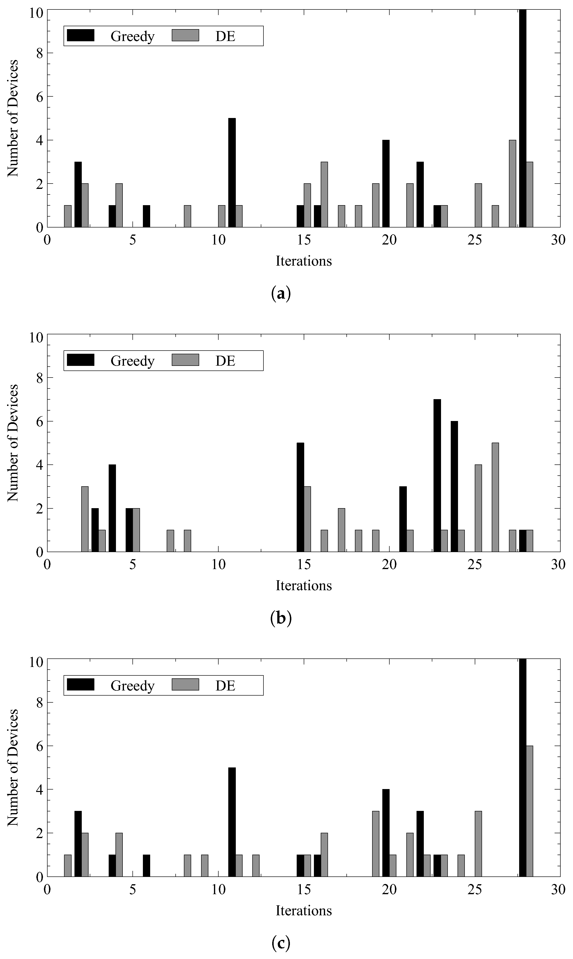
- We proposed two algorithms, greedy and DE, for different purposes. The greedy algorithm is designed to minimize the charging time and the DE algorithm can achieve a better performance for energy overflow minimization. The greedy algorithm attempts to charge devices as early as possible by rotating the direction of the directional antenna’s beam. The DE algorithm jointly considers the issue of battery overflow to reduce the number of fully charged devices at the same time.
- To gradually increase the number of fully charged devices, the problem of minimizing both energy overflow and charging time is formulated as a joint optimization problem. Therefore, the algorithm proposed for the optimization problem can pursue a charging schedule that may reduce the number of fully charged devices at the same time.
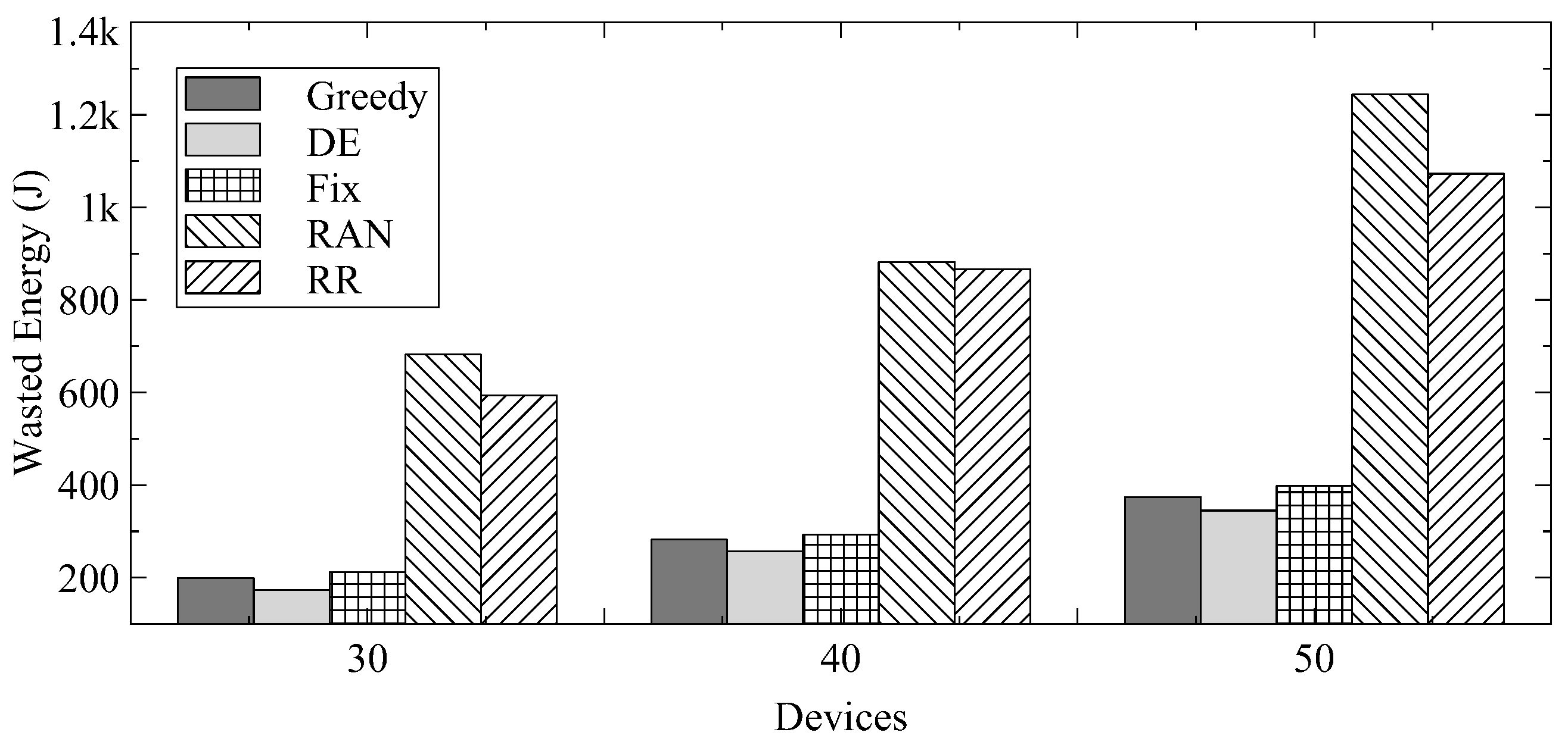
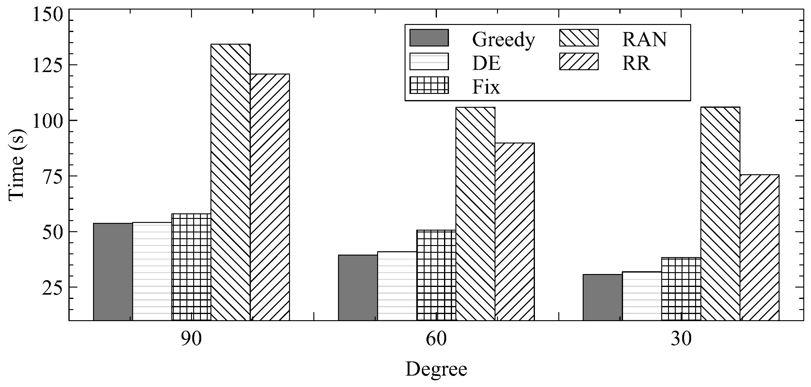
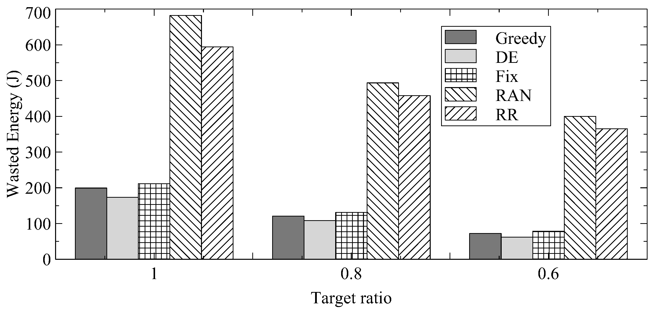
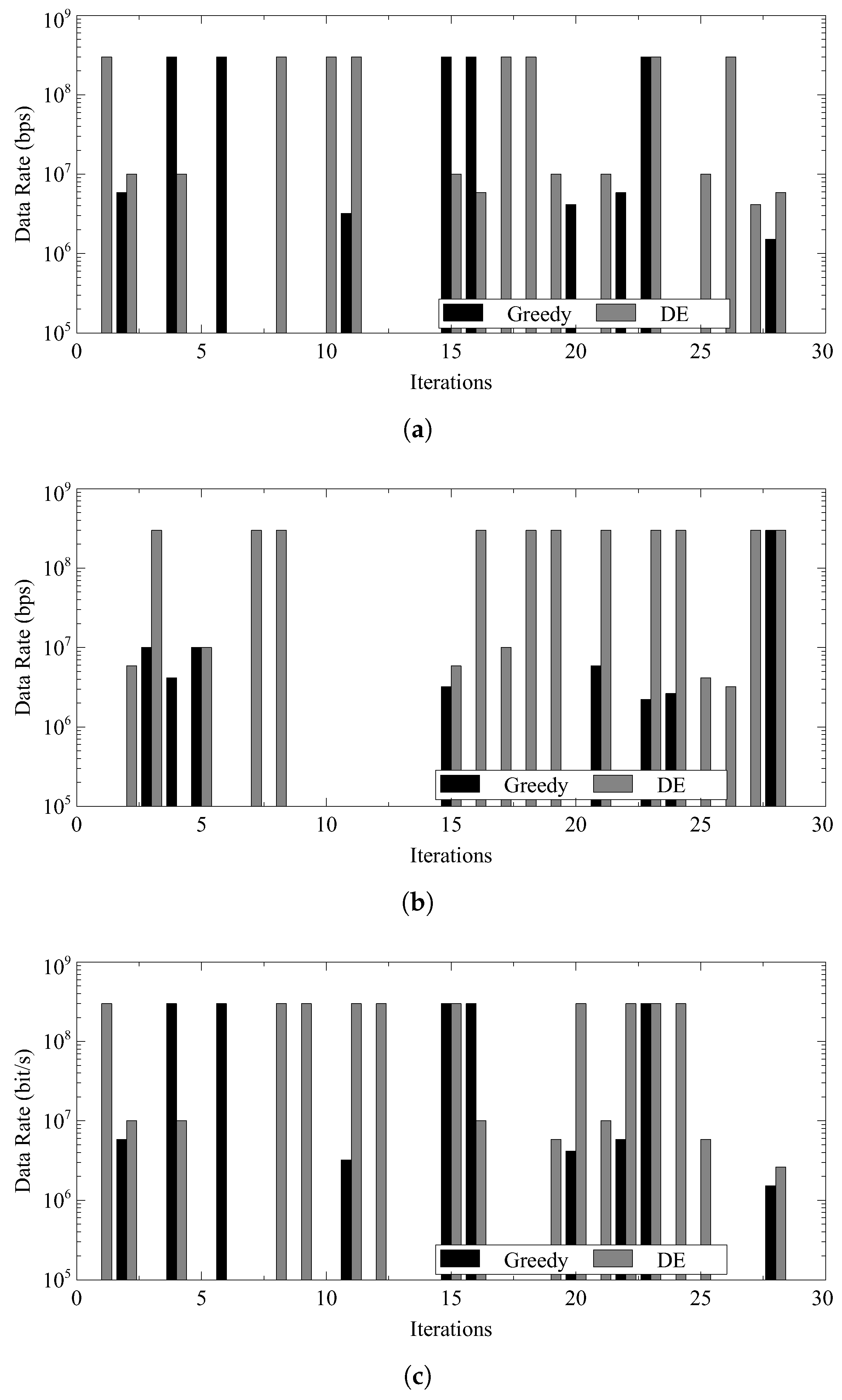
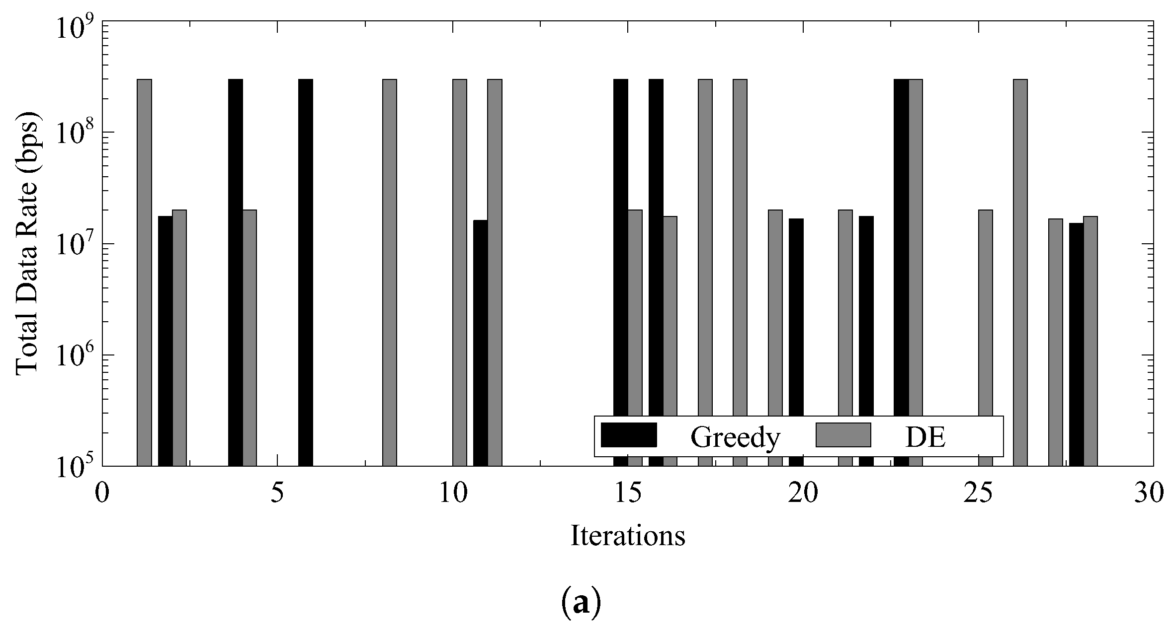
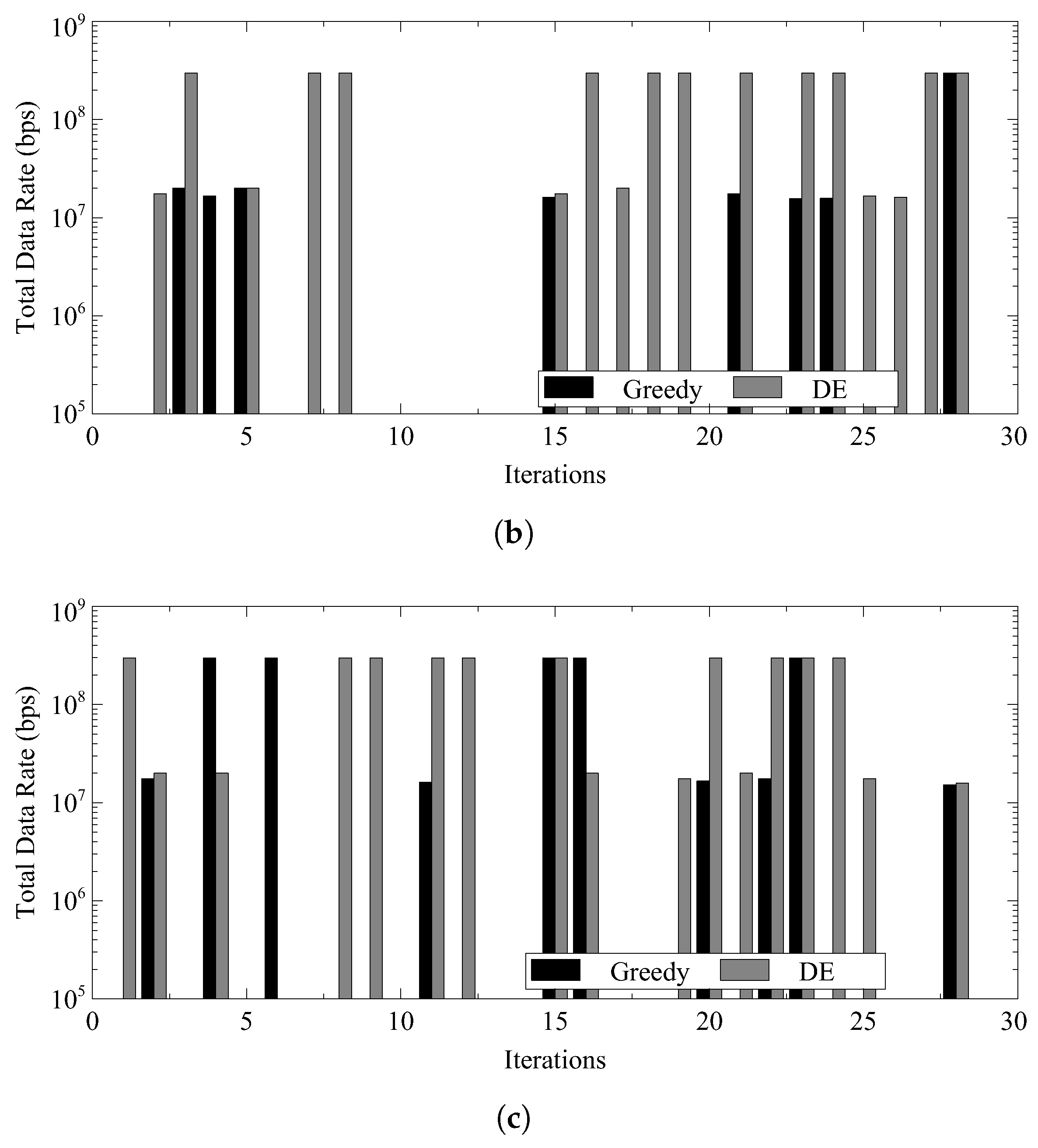
- We conduct a comprehensive performance evaluation to demonstrate the performance of our scheme. The experimental results show that both greedy and DE algorithms can achieve a short charging time and the proposed DE algorithm can further reduce the amount of energy wasted by charged devices. We also show that, by reducing the number of fully charged devices at the same time, the performance of data transmission can be improved.
2. Related Work
2.1. Energy Harvesting Applications
2.2. Improvement of Energy Harvesting
2.3. Beamforming
2.4. Research Gap
3. System Model
3.1. Architecture of RF Energy Harvesting
3.2. Channel Model
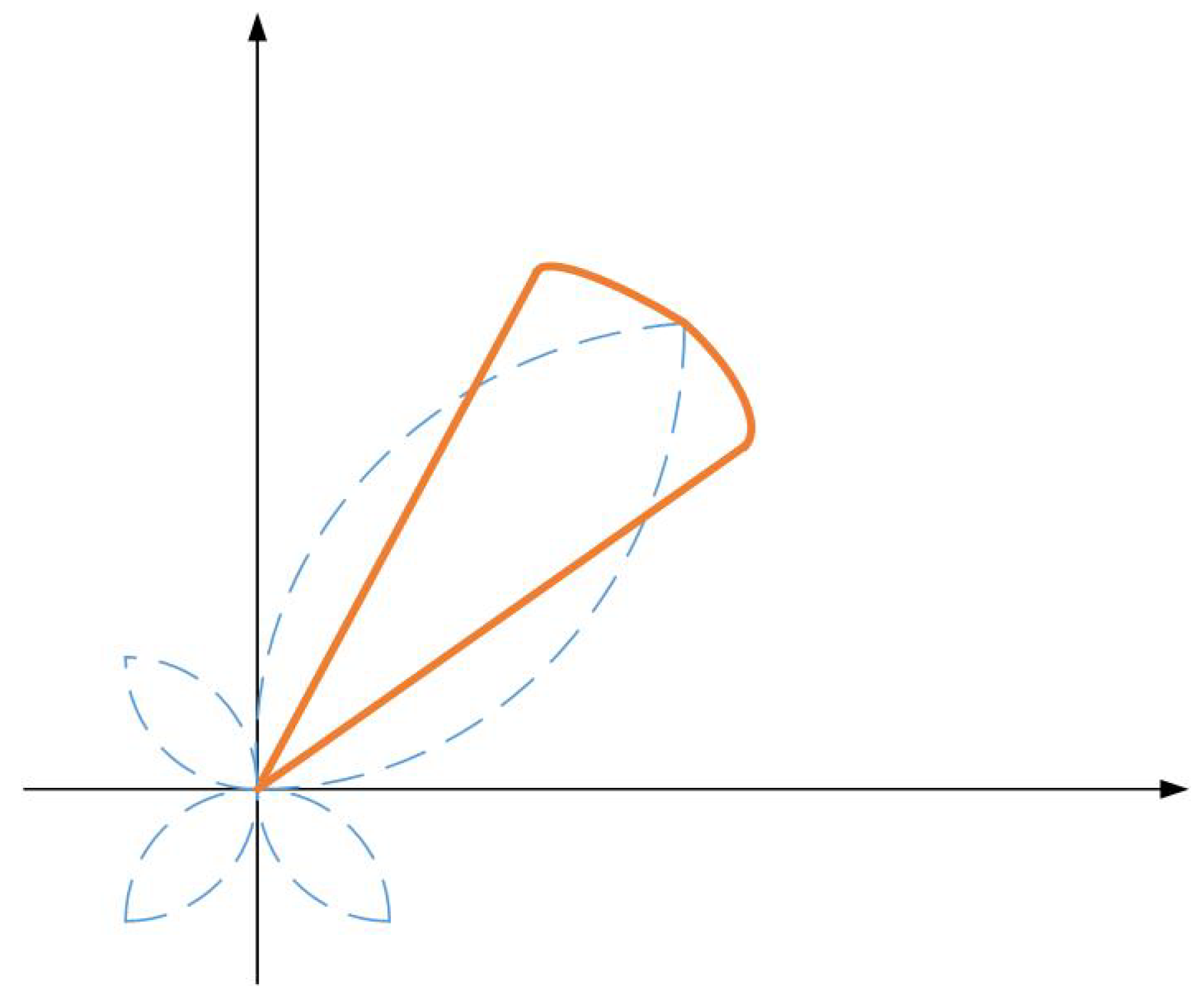
3.3. Antenna Model
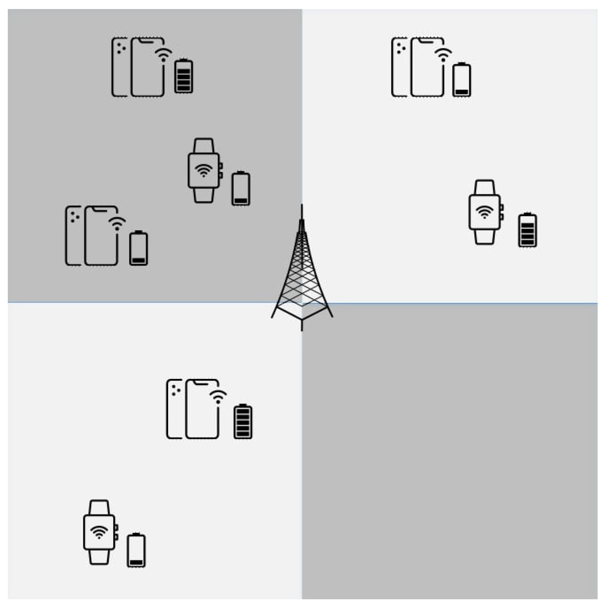
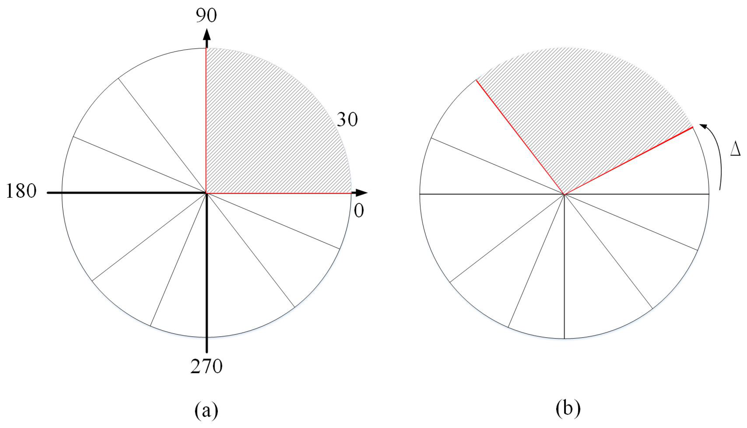
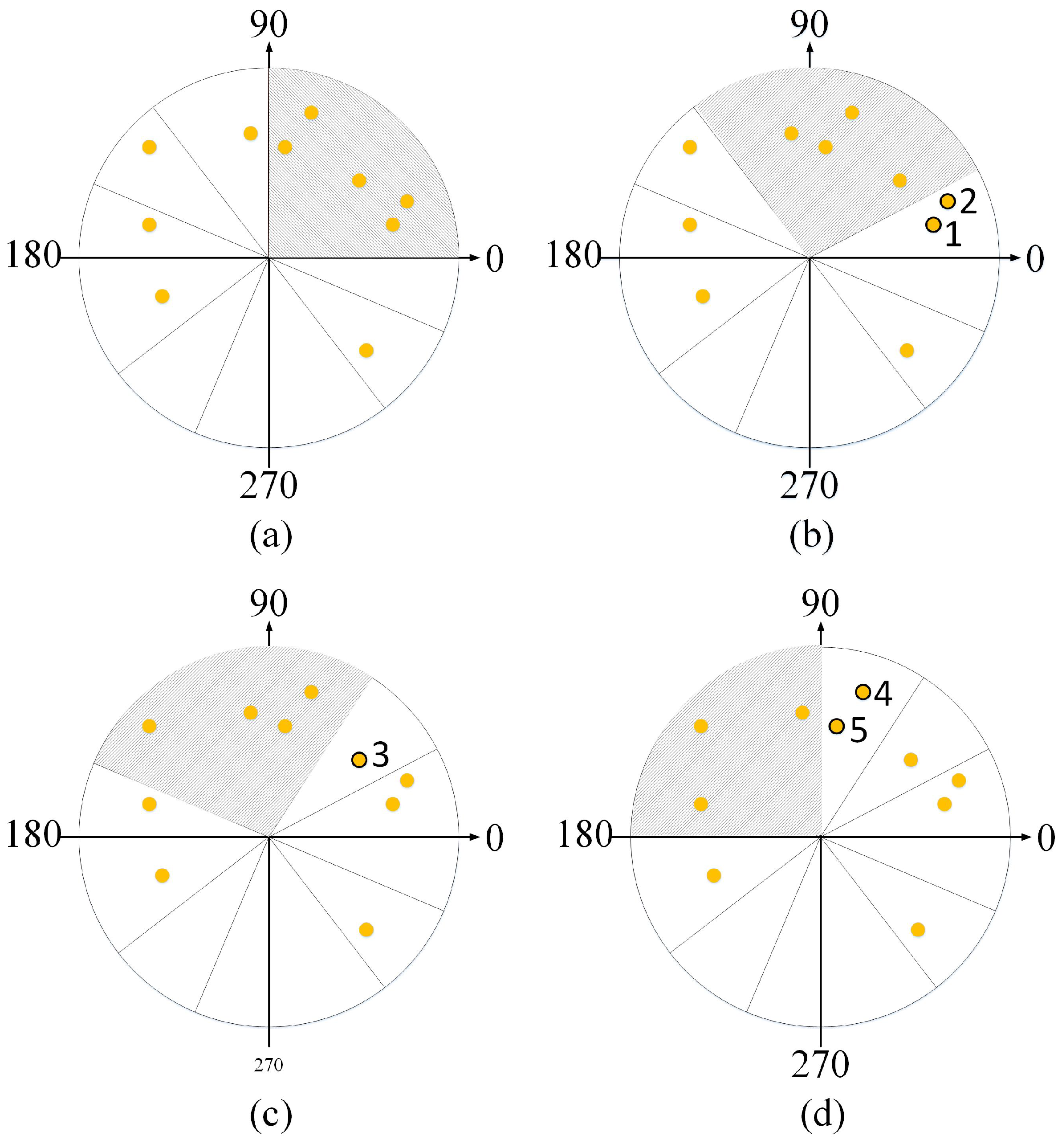
3.4. Sector Model
3.5. Problem Formulation
4. Energy Harvesting Using Directional Antenna
4.1. Greedy Algorithm
| Algorithm 1 Greedy |
|
4.2. Differential Evolution
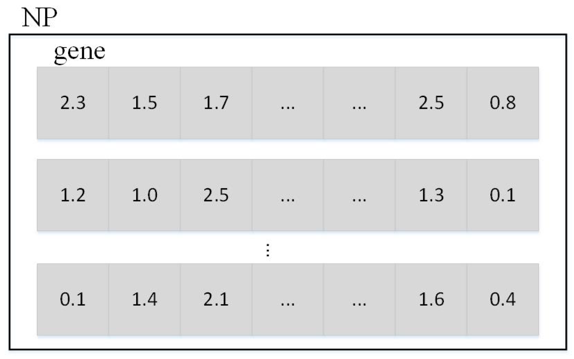
4.2.1. Initialization
4.2.2. Mutation
4.2.3. Crossover
4.2.4. Selection
4.2.5. DE Algorithm
| Algorithm 2 DE |
|
5. Simulation Results
5.1. Experiment Settings
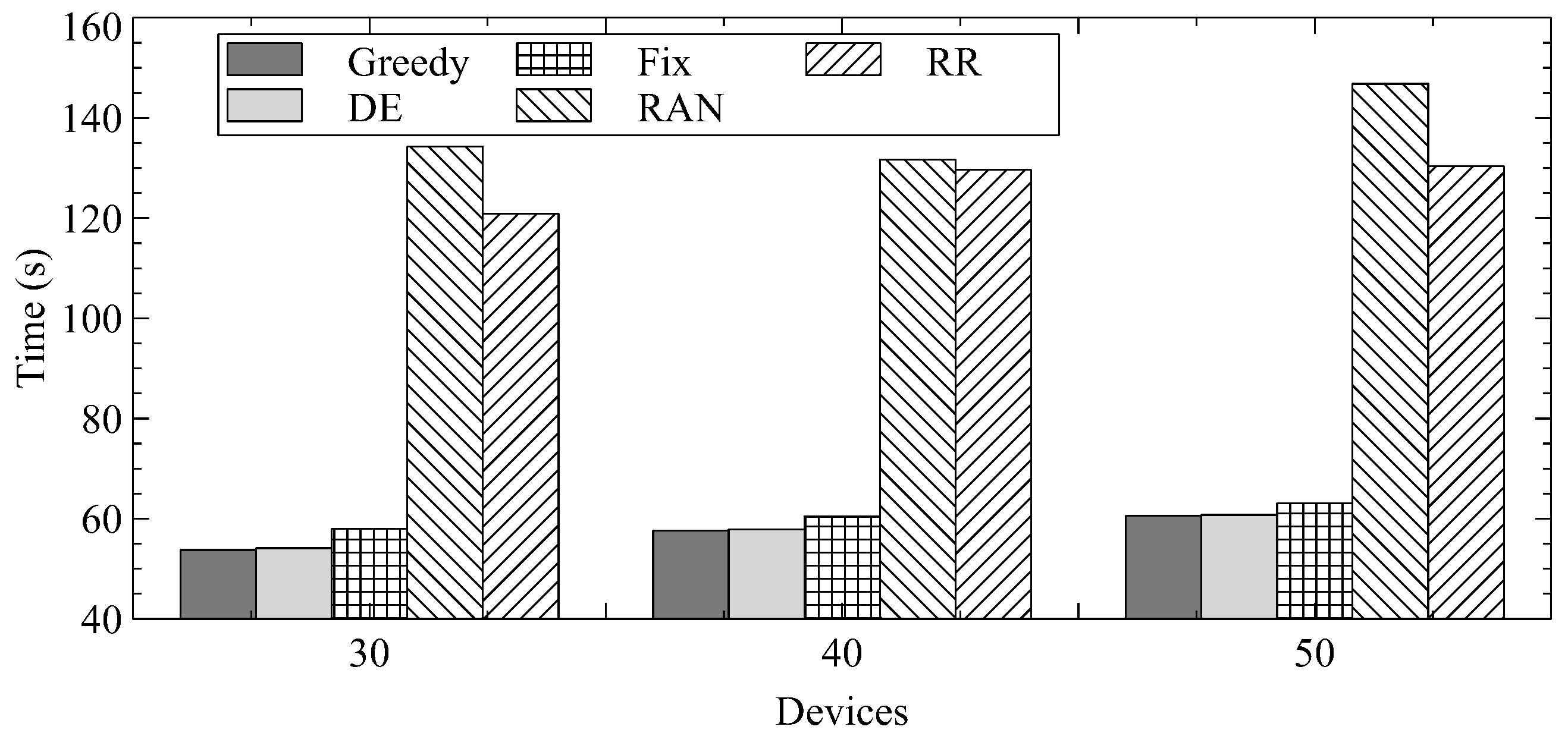
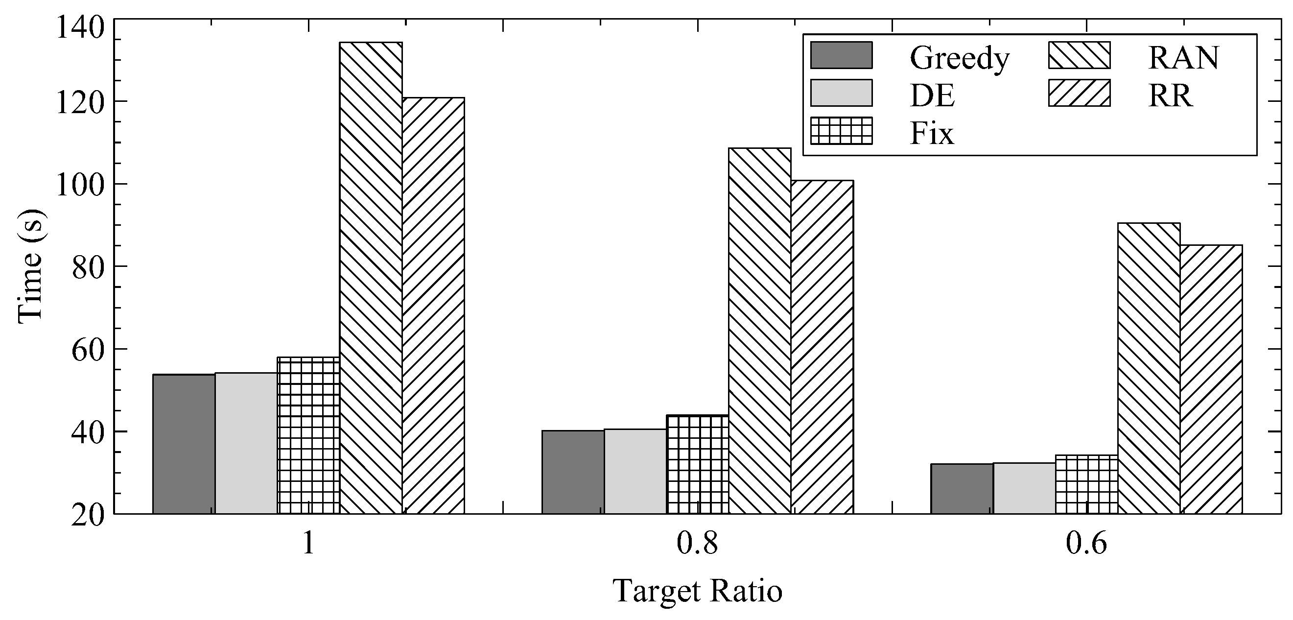
- Random (RAN): The AP randomly chooses any direction to transfer energy for one second until all devices are fully charged.
- Round Robin (RR): The AP transmits energy in counterclockwise order for one second until all devices are fully charged.
- Fix: The AP has one antenna for one fixed direction. The number of the sectors is equal to the number of antennas.
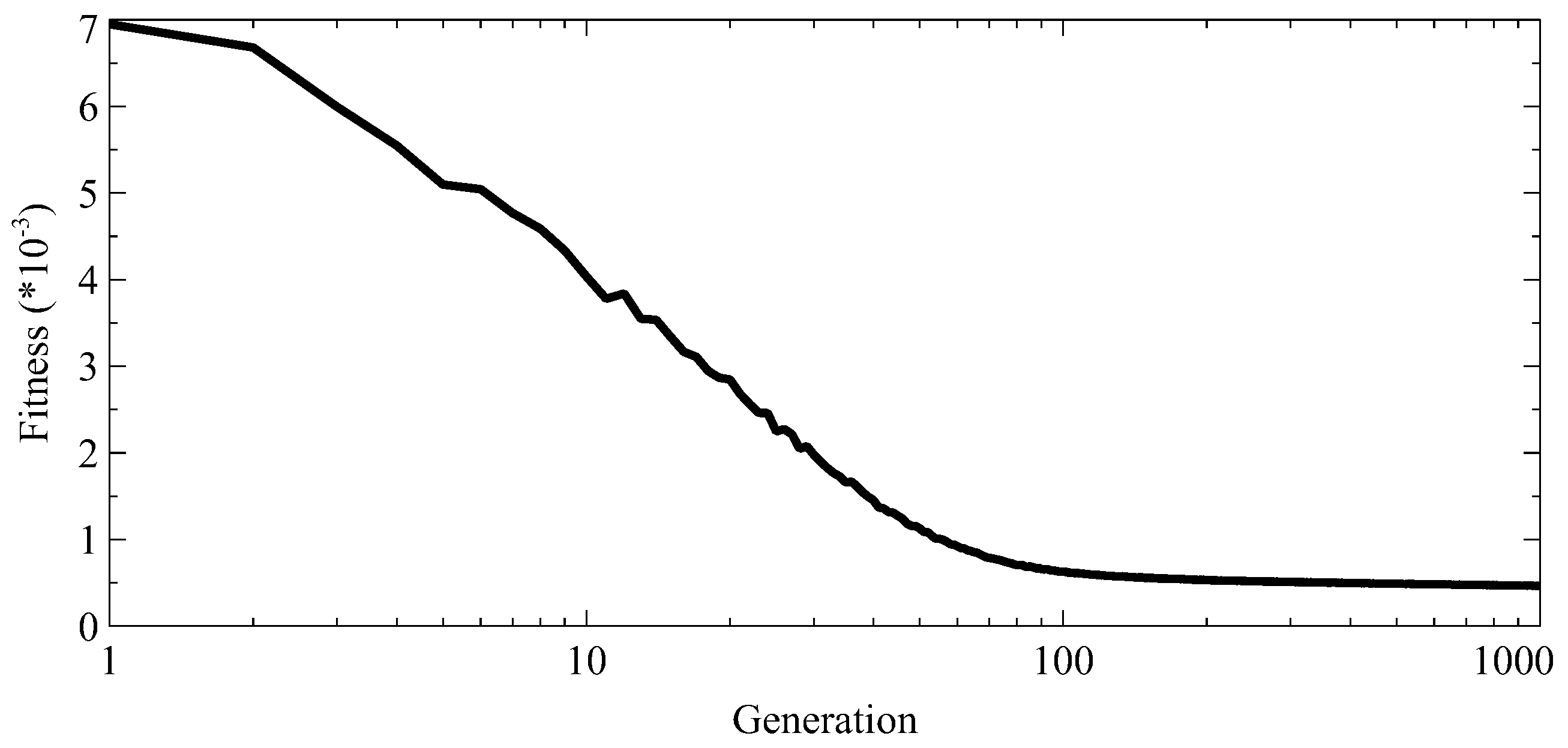
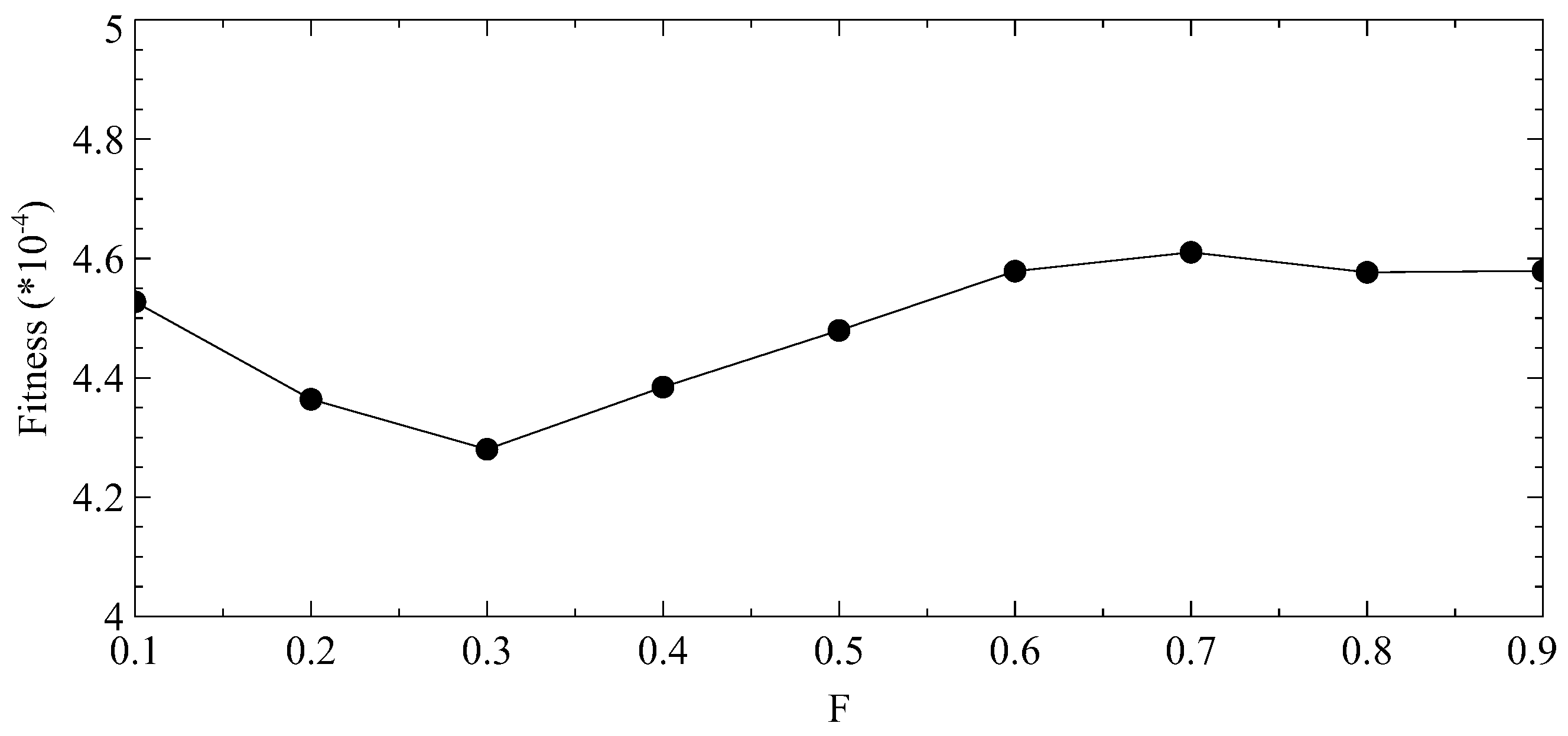
5.2. Parameters of DE
5.3. Comparative Performance Evaluation
5.3.1. Different Number of Devices
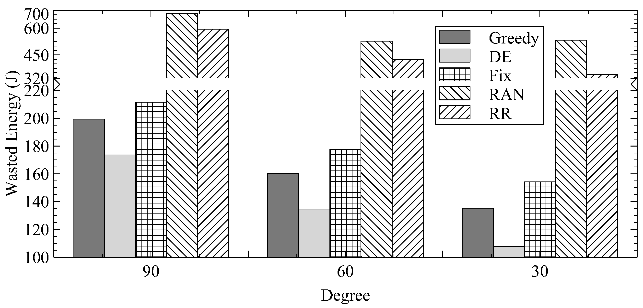
5.3.2. Different Transmission Angles
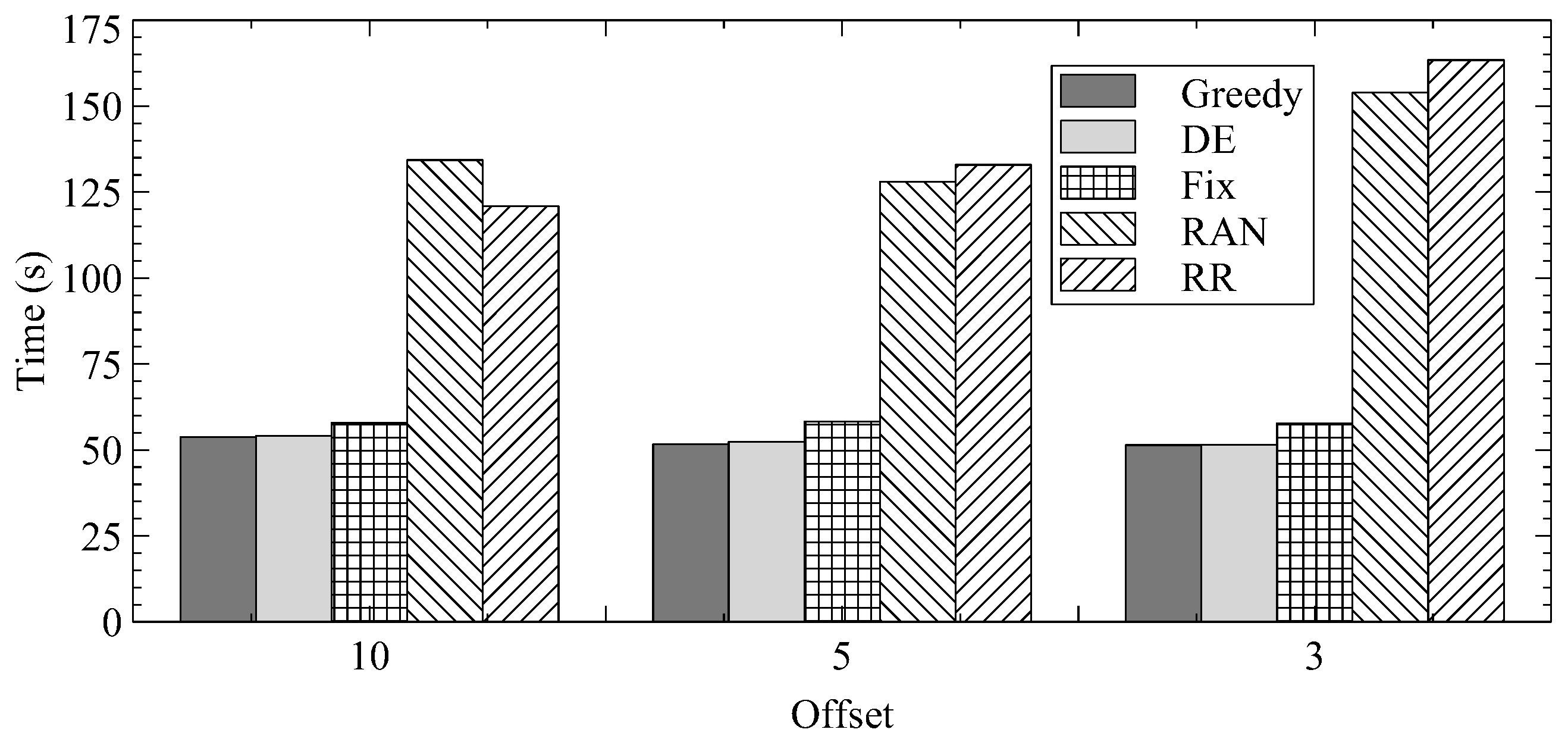
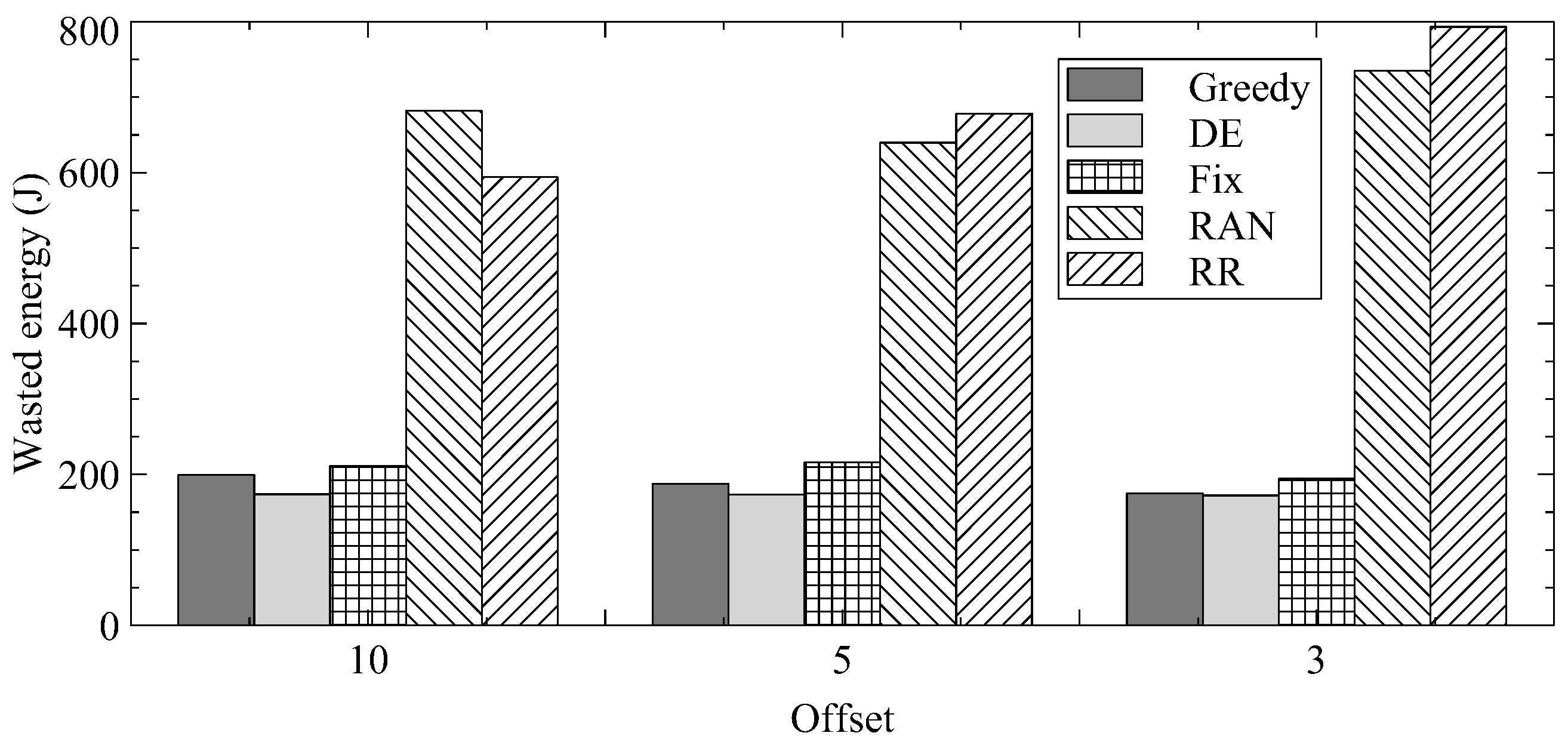
5.3.3. Different Offset Values
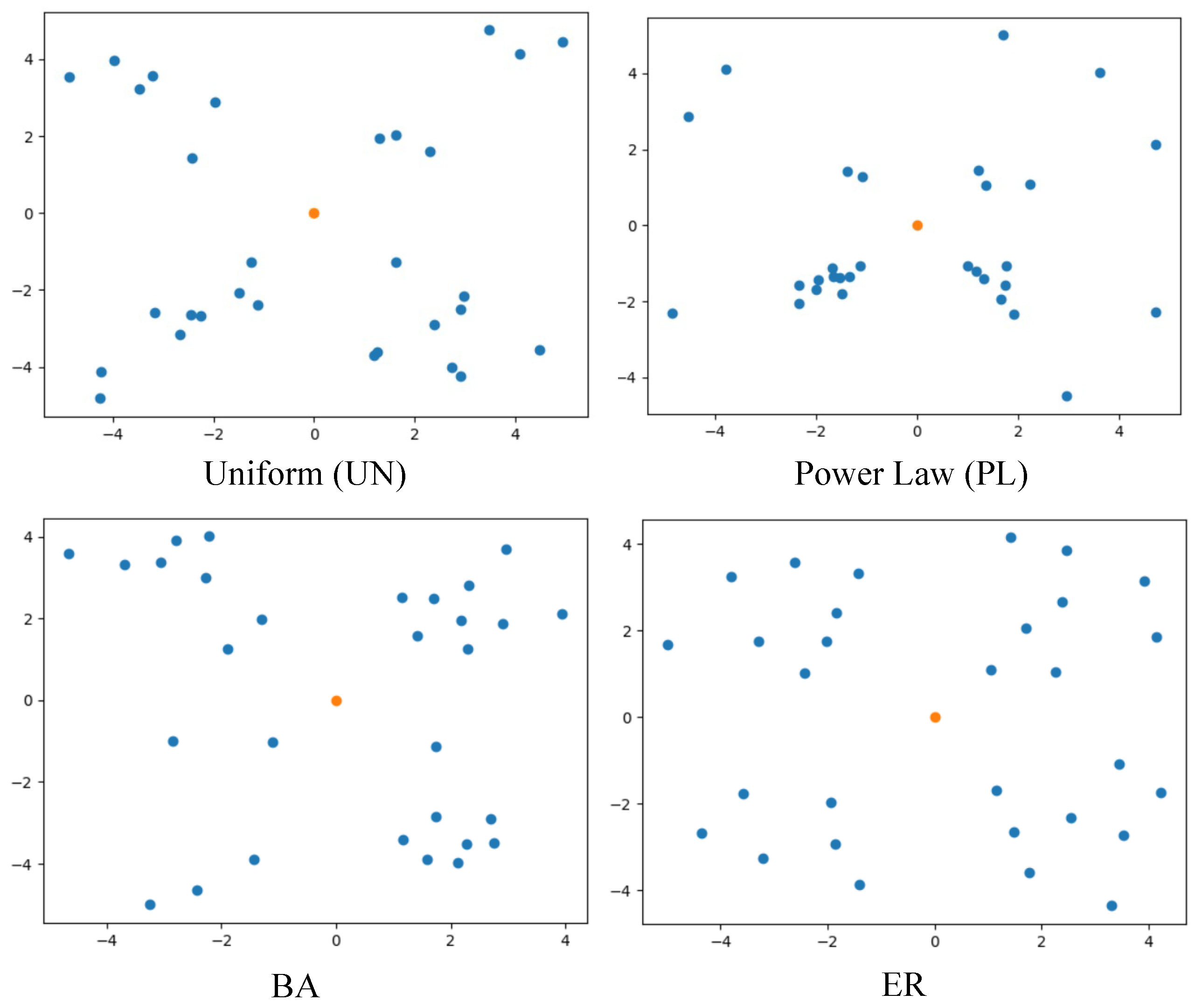
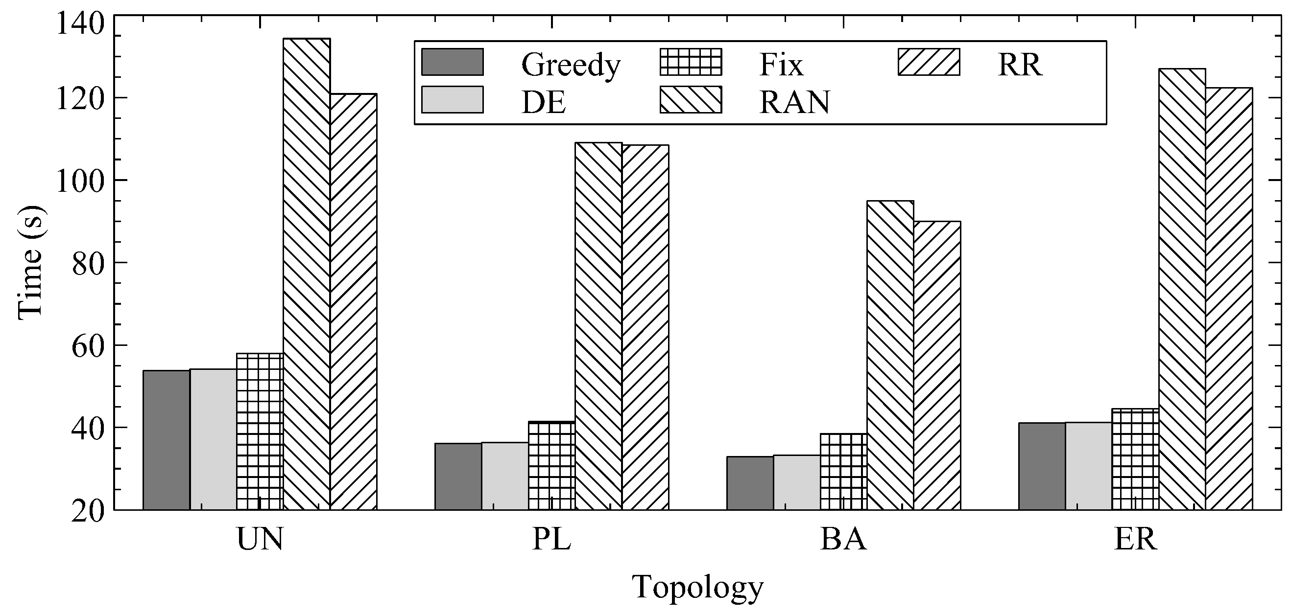
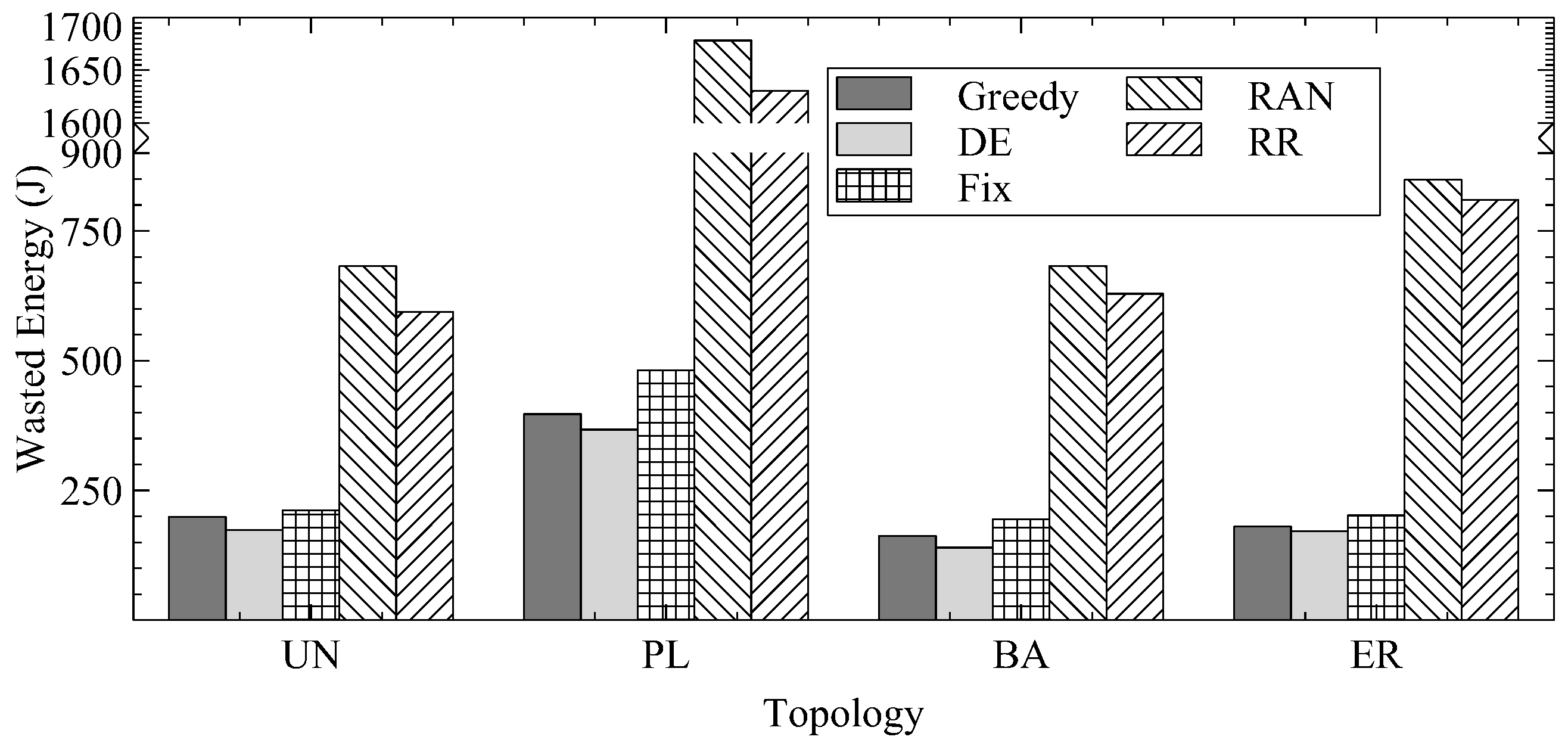
5.3.4. Different Topologies
- Uniform (UN): The nodes are evenly distributed in the region.
- Power Law (PL): There are more nodes in the center area.
- BA: There are fewer nodes in the center area.
- ER: Nodes are uniformly distributed at the region while any two nodes are not close to each other.
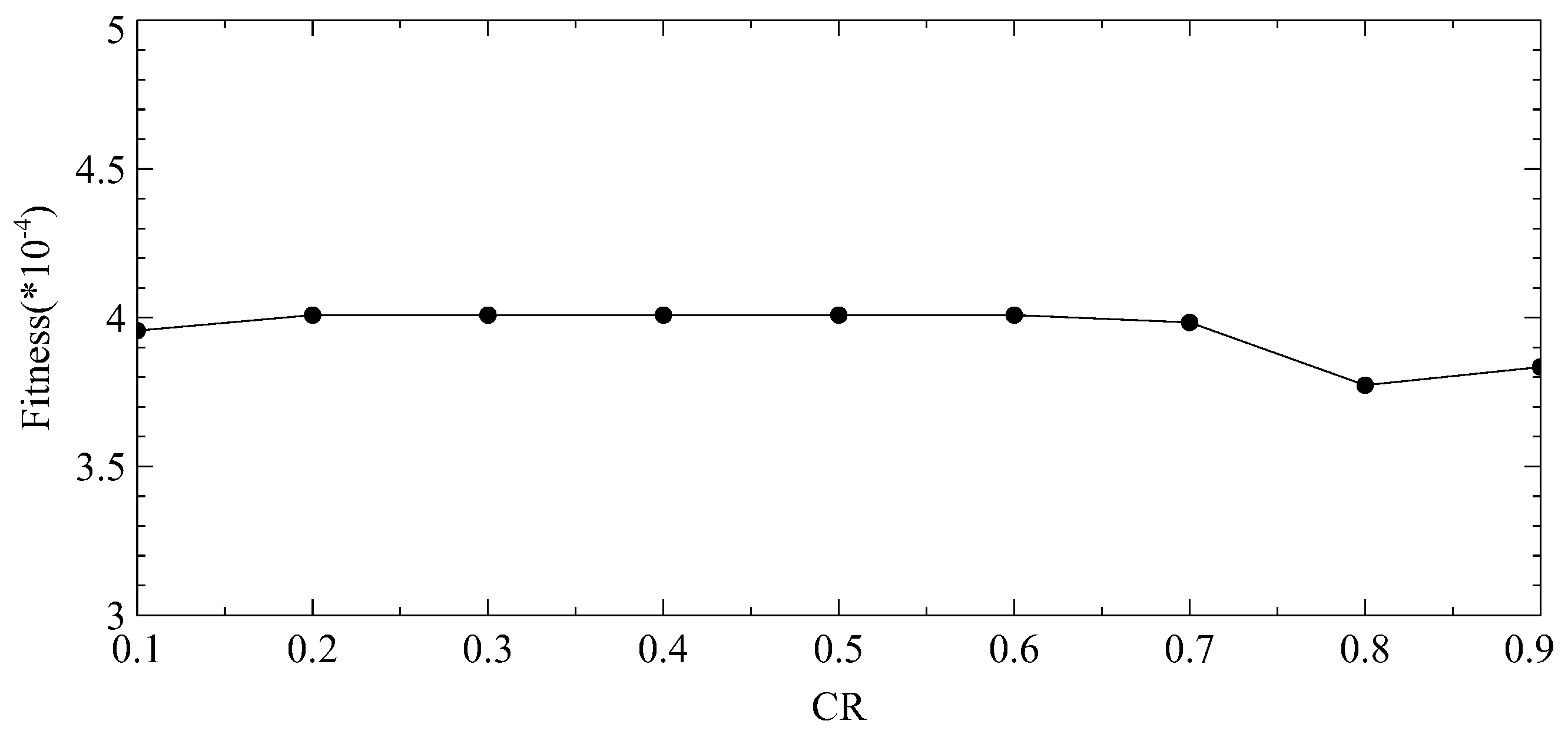
5.3.5. Different Charging Ratios
5.4. Time Distribution of Fully Charged Devices
6. Conclusions
Author Contributions
Funding
Data Availability Statement
Conflicts of Interest
References
- Tran, V.H.; Misra, A.; Xiong, J.; Balan, R.K. WiWear: Wearable Sensing via Directional WiFi Energy Harvesting. In Proceedings of the 2019 IEEE International Conference on Pervasive Computing and Communications (PerCom), Kyoto, Japan, 11–15 March 2019; pp. 1–10. [Google Scholar] [CrossRef]
- Park, C.; Chou, P.H. AmbiMax: Autonomous Energy Harvesting Platform for Multi-Supply Wireless Sensor Nodes. In Proceedings of the 2006 3rd Annual IEEE Communications Society on Sensor and Ad Hoc Communications and Networks, Reston, VA, USA, 28 September 2006; Volume 1, pp. 168–177. [Google Scholar] [CrossRef]
- Fan, K.W.; Zheng, Z.; Sinha, P. Steady and Fair Rate Allocation for Rechargeable Sensors in Perpetual Sensor Networks. In Proceedings of the SenSys ’08: 6th ACM Conference on Embedded Network Sensor Systems, Raleigh, NC, USA, 5–7 November 2008; Association for Computing Machinery: New York, NY, USA, 2008; pp. 239–252. [Google Scholar] [CrossRef]
- Meninger, S.; Mur-Miranda, J.; Amirtharajah, R.; Chandrakasan, A.; Lang, J. Vibration-to-electric energy conversion. In IEEE Transactions on Very Large Scale Integration (VLSI) Systems; IEEE: New York, NY, USA, 2001; Volume 9, pp. 64–76. [Google Scholar] [CrossRef]
- Wang, Y.; Yang, K.; Wan, W.; Zhang, Y.; Liu, Q. Energy-Efficient Data and Energy Integrated Management Strategy for IoT Devices Based on RF Energy Harvesting. IEEE Internet Things J. 2021, 8, 13640–13651. [Google Scholar] [CrossRef]
- Galinina, O.; Tabassum, H.; Mikhaylov, K.; Andreev, S.; Hossain, E.; Koucheryavy, Y. On feasibility of 5G-grade dedicated RF charging technology for wireless-powered wearables. IEEE Wirel. Commun. 2016, 23, 28–37. [Google Scholar] [CrossRef]
- Ko, H.; Pack, S. OB-DETA: Observation-based directional energy transmission algorithm in energy harvesting networks. J. Commun. Netw. 2019, 21, 168–176. [Google Scholar] [CrossRef]
- Shi, L.; Ye, Y.; Chu, X.; Lu, G. Computation Energy Efficiency Maximization for a NOMA-Based WPT-MEC Network. IEEE Internet Things J. 2021, 8, 10731–10744. [Google Scholar] [CrossRef]
- Wang, N.; Wu, J.; Dai, H. Bundle Charging: Wireless Charging Energy Minimization in Dense Wireless Sensor Networks. In Proceedings of the 2019 IEEE 39th International Conference on Distributed Computing Systems (ICDCS), Dallas, TX, USA, 7–10 July 2019; pp. 810–820. [Google Scholar] [CrossRef]
- Prawiro, S.Y.; Murti, M.A. Wireless power transfer solution for smart charger with RF energy harvesting in public area. In Proceedings of the 2018 IEEE 4th World Forum on Internet of Things (WF-IoT), Singapore, 5–8 February 2018; pp. 103–106. [Google Scholar] [CrossRef]
- Sandhu, M.M. PhD Forum Abstract: Energy Harvesting based Sensing for the Batteryless IoT. In Proceedings of the 2020 19th ACM/IEEE International Conference on Information Processing in Sensor Networks (IPSN), Sydney, NSW, Australia, 21–24 April 2020; pp. 373–374. [Google Scholar] [CrossRef]
- Nguyen, T.D.; Khan, J.Y.; Ngo, D.T. A Distributed Energy-Harvesting-Aware Routing Algorithm for Heterogeneous IoT Networks. IEEE Trans. Green Commun. Netw. 2018, 2, 1115–1127. [Google Scholar] [CrossRef]
- Zhang, H.; Lu, N.; Li, J.; Song, R.; Liu, Y. Lifetime Analysis for Ambient RF Energy Harvesting IoT Node. In Proceedings of the 2019 IEEE 5th International Conference on Computer and Communications (ICCC), Chengdu, China, 6–9 December 2019; pp. 2157–2161. [Google Scholar] [CrossRef]
- Wen, Z.; Yang, K.; Liu, X.; Li, S.; Zou, J. Joint Offloading and Computing Design in Wireless Powered Mobile-Edge Computing Systems With Full-Duplex Relaying. IEEE Access 2018, 6, 72786–72795. [Google Scholar] [CrossRef]
- Ko, H.; Pack, S. Phase-Aware Directional Energy Transmission Algorithm in Multiple Directional RF Energy Source Environments. IEEE Trans. Veh. Technol. 2019, 68, 359–367. [Google Scholar] [CrossRef]
- Zhang, K.; Ahn, J.H.; Lee, T.J.; Zhao, P. AP scheduling protocol for power beacon with directional antenna in Energy Harvesting Networks. In Proceedings of the 2017 International Conference on Applied System Innovation (ICASI), Sapporo, Japan, 13–17 May 2017; pp. 906–909. [Google Scholar] [CrossRef]
- Bi, S.; Zhang, Y.J. Computation Rate Maximization for Wireless Powered Mobile-Edge Computing With Binary Computation Offloading. IEEE Trans. Wirel. Commun. 2018, 17, 4177–4190. [Google Scholar] [CrossRef]
- Lee, D.J.; Lee, S.J.; Hwang, I.J.; Lee, W.S.; Yu, J.W. Hybrid Power Combining Rectenna Array for Wide Incident Angle Coverage in RF Energy Transfer. IEEE Trans. Microw. Theory Tech. 2017, 65, 3409–3418. [Google Scholar] [CrossRef]
- Shen, S.; Zhang, Y.; Chiu, C.Y.; Murch, R. Directional Multiport Ambient RF Energy-Harvesting System for the Internet of Things. IEEE Internet Things J. 2021, 8, 5850–5865. [Google Scholar] [CrossRef]
- Sun, Y.; Song, C.; Yu, S.; Liu, Y.; Pan, H.; Zeng, P. Energy-Efficient Task Offloading Based on Differential Evolution in Edge Computing System With Energy Harvesting. IEEE Access 2021, 9, 16383–16391. [Google Scholar] [CrossRef]
- Zhang, Z.; Cai, Y.; Zhang, D. Solving Ordinary Differential Equations With Adaptive Differential Evolution. IEEE Access 2020, 8, 128908–128922. [Google Scholar] [CrossRef]
- Li, T.; Yang, F.; Zhang, D.; Zhai, L. Computation Scheduling of Multi-Access Edge Networks Based on the Artificial Fish Swarm Algorithm. IEEE Access 2021, 9, 74674–74683. [Google Scholar] [CrossRef]
- Min, M.; Xiao, L.; Chen, Y.; Cheng, P.; Wu, D.; Zhuang, W. Learning-Based Computation Offloading for IoT Devices With Energy Harvesting. IEEE Trans. Veh. Technol. 2019, 68, 1930–1941. [Google Scholar] [CrossRef]
- Luo, Y.; Chin, K.W. Learning to Charge RF-Energy Harvesting Devices in WiFi Networks. IEEE Syst. J. 2021, 15, 5516–5525. [Google Scholar] [CrossRef]
- Ren, H.; Chin, K.W. A Reinforcement Learning Approach to Optimize Energy Usage in RF-Charging Sensor Networks. IEEE Trans. Green Commun. Netw. 2021, 5, 526–539. [Google Scholar] [CrossRef]
- Alsaba, Y.; Rahim, S.K.A.; Leow, C.Y. Beamforming in Wireless Energy Harvesting Communications Systems: A Survey. IEEE Commun. Surv. Tutorials 2018, 20, 1329–1360. [Google Scholar] [CrossRef]
- Hiep, P.T.; Hoang, T.M. Non-orthogonal multiple access and beamforming for relay network with RF energy harvesting. ICT Express 2020, 6, 11–15. [Google Scholar] [CrossRef]
- Li, C.; Tang, J.; Zhang, Y.; Yan, X.; Luo, Y. Energy efficient computation offloading for nonorthogonal multiple access assisted mobile edge computing with energy harvesting devices. Comput. Netw. 2019, 164, 106890. [Google Scholar] [CrossRef]
- Wang, S.; Zhao, L.; Liang, K.; Chu, X.; Jiao, B. Energy beamforming for full-duplex wireless-powered communication networks. Phys. Commun. 2018, 26, 134–140. [Google Scholar] [CrossRef]
- Guo, F. Scikit-opt. 2019. Available online: https://github.com/guofei9987/scikit-opt/ (accessed on 1 July 2023).
- Hu, H.C.; Wang, P.C. Computation Offloading Game for Multi-Channel Wireless Sensor Networks. Sensors 2022, 22, 8718. [Google Scholar] [CrossRef] [PubMed]


| Reference | Beamforming | Battery | Research Goal |
|---|---|---|---|
| [5] | None | No | Minimizing energy consumption with single |
| WET source | |||
| [7] | None | Yes | Optimizing sectors for single WET source |
| [15] | None | Yes | Optimizing directions and phases of multiple |
| WET sources | |||
| [20,22] | None | Yes | Optimizing WET time period for computation |
| Tasks | |||
| [23] | None | Yes | Predicting WET for computation tasks |
| [24] | None | Yes | Optimizing WET time period for data |
| Transmission | |||
| [25] | None | Yes | Optimizing WET time period and avoiding |
| energy overflow | |||
| [28] | Yes | Yes | Minimizing energy consumption with single |
| WET source | |||
| [29] | Yes | No | Optimizing WET time period for data |
| transmission |
| Parameters | Value |
|---|---|
| Topology | Uniform |
| Number of Devices | |
| The minimum device distance | 1 m |
| The maximum device distance | m |
| Offset value | degree |
| Transmission angle | degree |
| 5 W | |
| 5 J | |
| Conversion rate | |
| Population size NP | 50 |
| Scaling factor F | |
| Hybridization probability CR | |
| Upper bound | |
| Lower bound | 0 |
| Generation | 1000 |
Disclaimer/Publisher’s Note: The statements, opinions and data contained in all publications are solely those of the individual author(s) and contributor(s) and not of MDPI and/or the editor(s). MDPI and/or the editor(s) disclaim responsibility for any injury to people or property resulting from any ideas, methods, instructions or products referred to in the content. |
© 2023 by the authors. Licensee MDPI, Basel, Switzerland. This article is an open access article distributed under the terms and conditions of the Creative Commons Attribution (CC BY) license (https://creativecommons.org/licenses/by/4.0/).
Share and Cite
Chang, H.-C.; Lin, H.-T.; Wang, P.-C. Wireless Energy Harvesting for Internet-of-Things Devices Using Directional Antennas. Future Internet 2023, 15, 301. https://doi.org/10.3390/fi15090301
Chang H-C, Lin H-T, Wang P-C. Wireless Energy Harvesting for Internet-of-Things Devices Using Directional Antennas. Future Internet. 2023; 15(9):301. https://doi.org/10.3390/fi15090301
Chicago/Turabian StyleChang, Hsiao-Ching, Hsing-Tsung Lin, and Pi-Chung Wang. 2023. "Wireless Energy Harvesting for Internet-of-Things Devices Using Directional Antennas" Future Internet 15, no. 9: 301. https://doi.org/10.3390/fi15090301
APA StyleChang, H.-C., Lin, H.-T., & Wang, P.-C. (2023). Wireless Energy Harvesting for Internet-of-Things Devices Using Directional Antennas. Future Internet, 15(9), 301. https://doi.org/10.3390/fi15090301