
A Hybrid Neural Ordinary Differential Equation Based Digital Twin Modeling and Online Diagnosis for an Industrial Cooling Fan


Abstract
:1. Introduction
2. Methodology
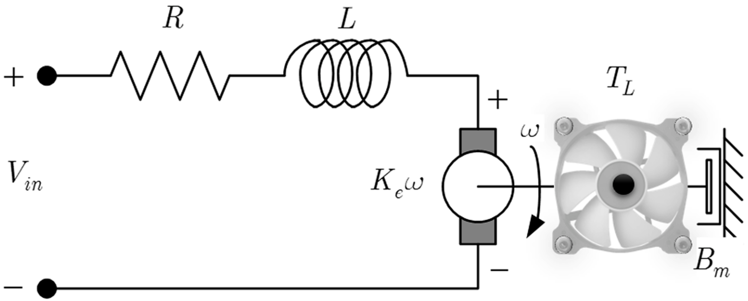
2.1. Cooling Fan System Dynamics
2.2. Filtering Operator Method
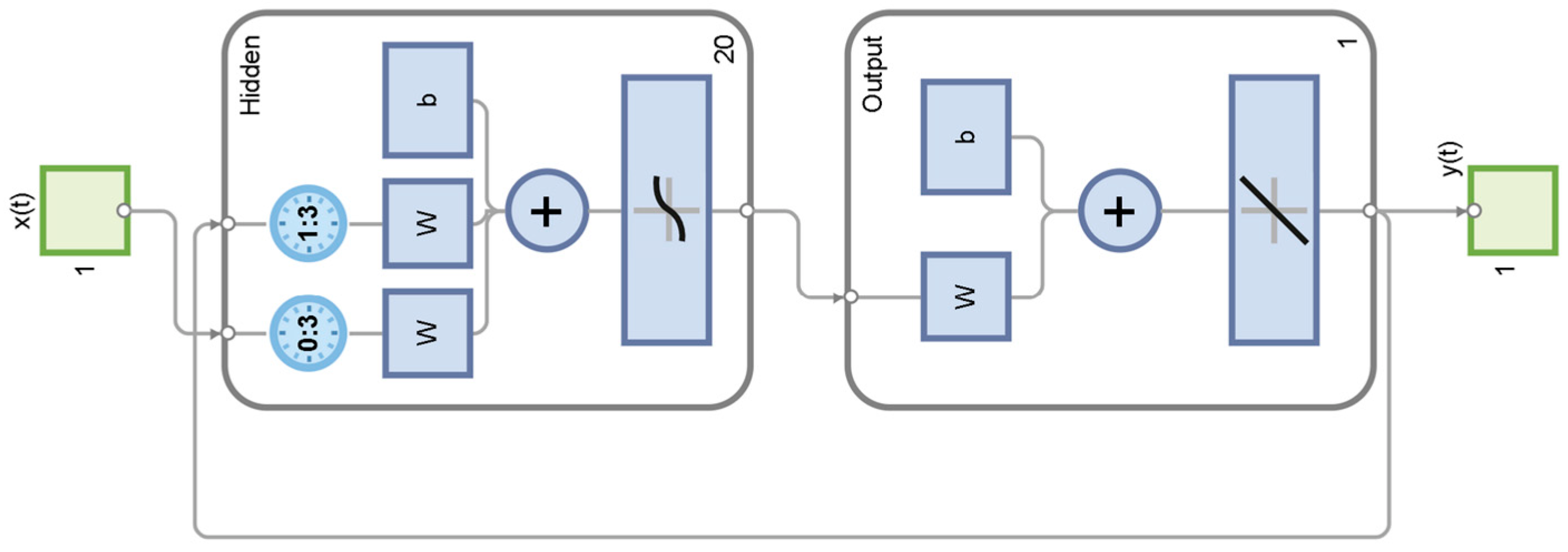
2.3. Recurrent Neural Network
2.4. Neural Ordinary Differential Equation
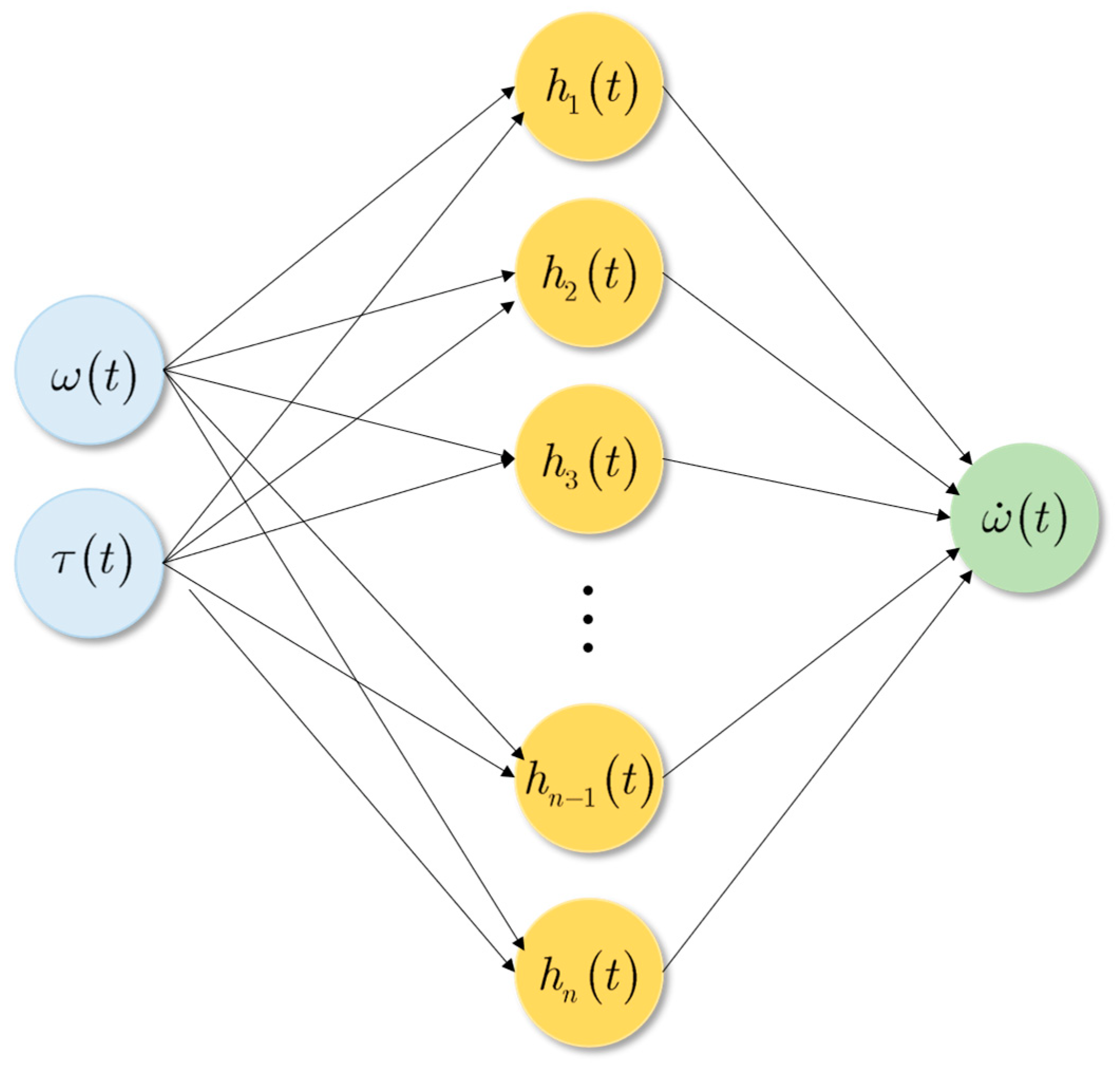
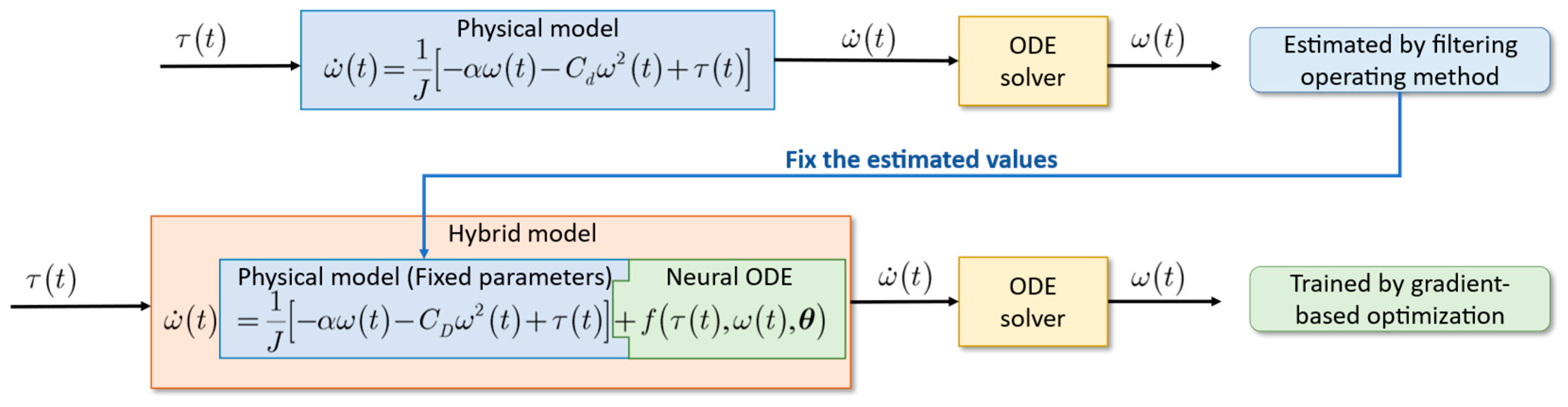
2.5. Hybrid Neural Ordinary Differential Equation
3. Literature Review
4. Digital Twins Derivation
4.1. Problem Formulation
4.2. Structure of Digital Twins
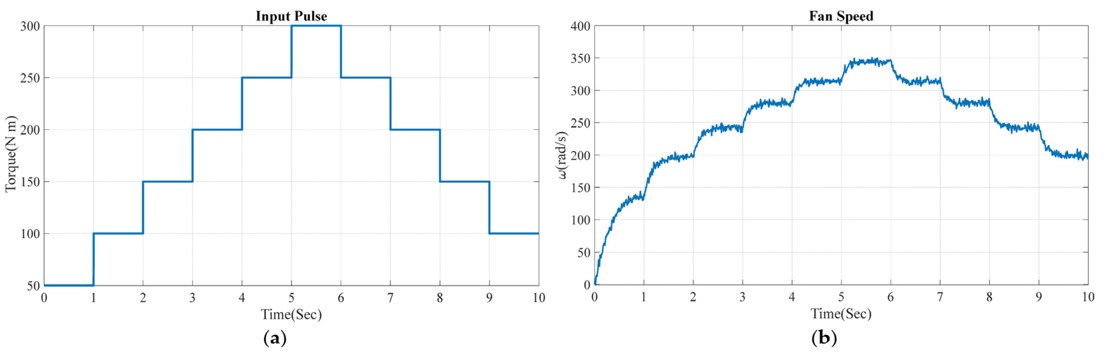
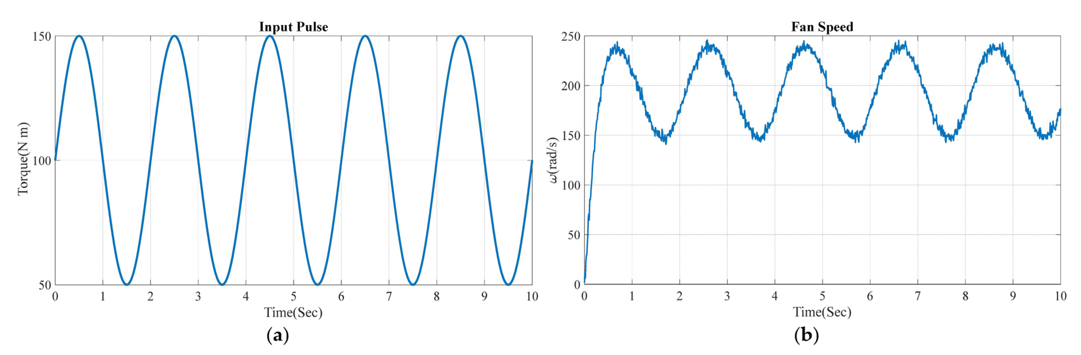
4.3. Numerical Simulation
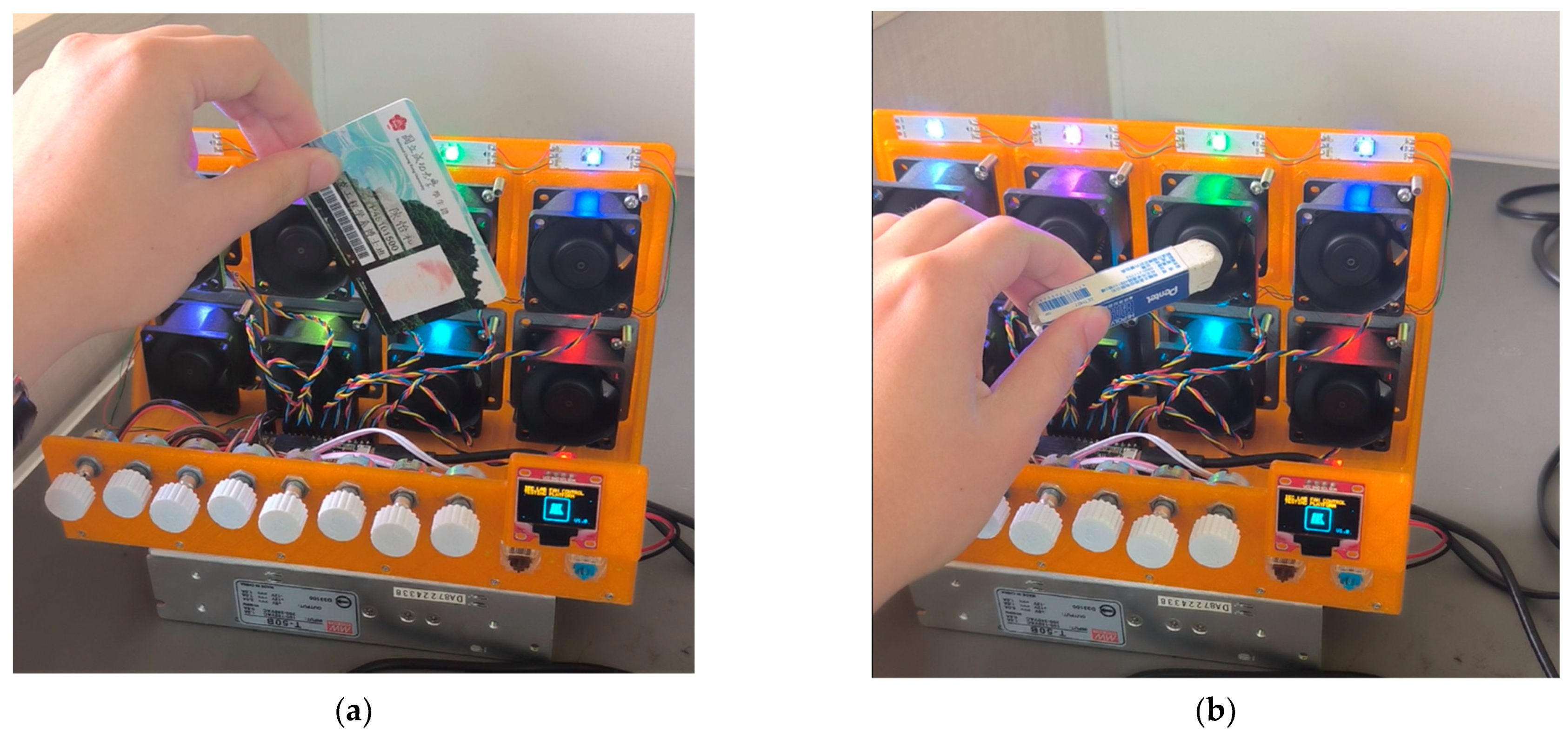
4.4. Experiment Validation
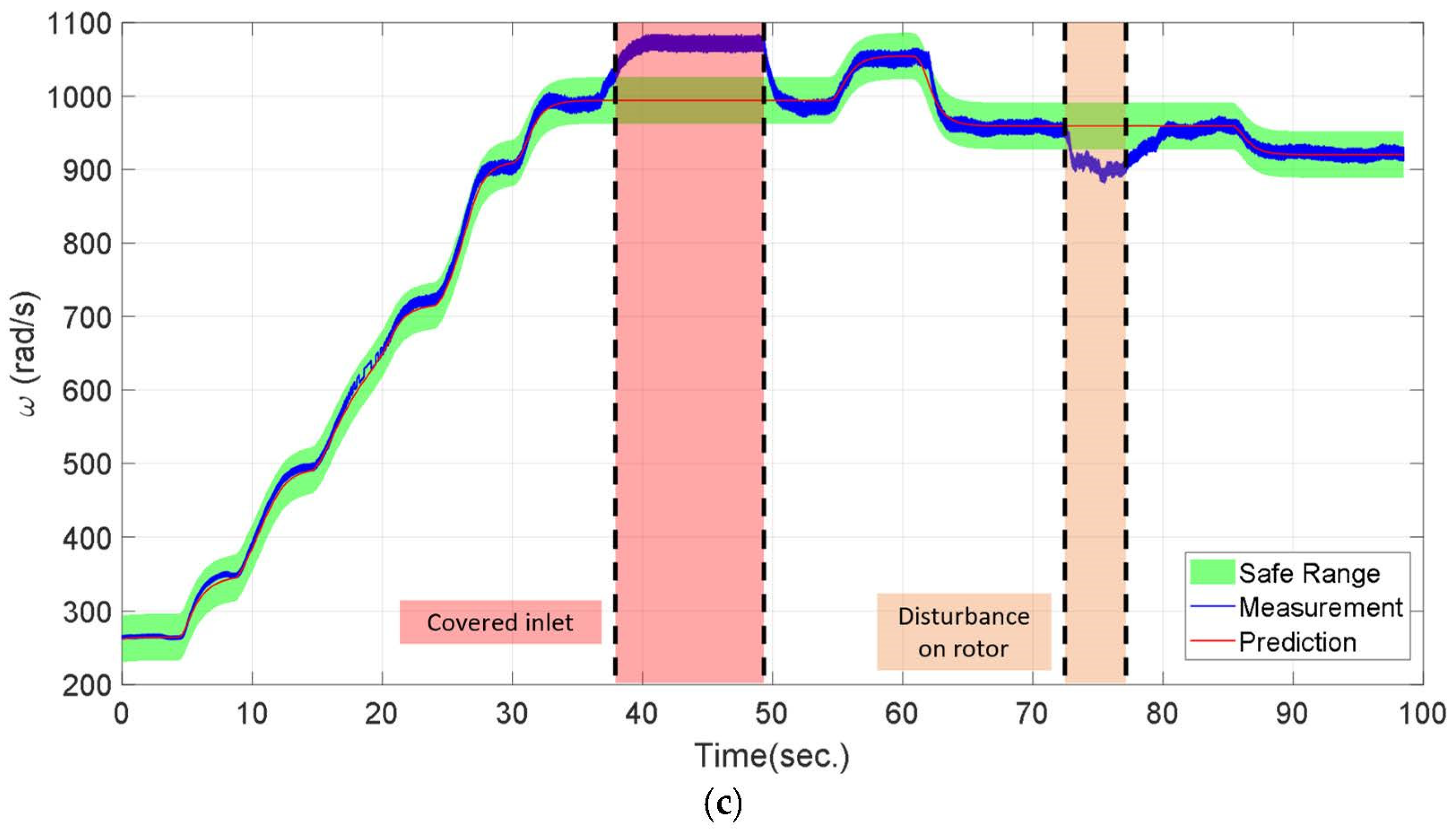
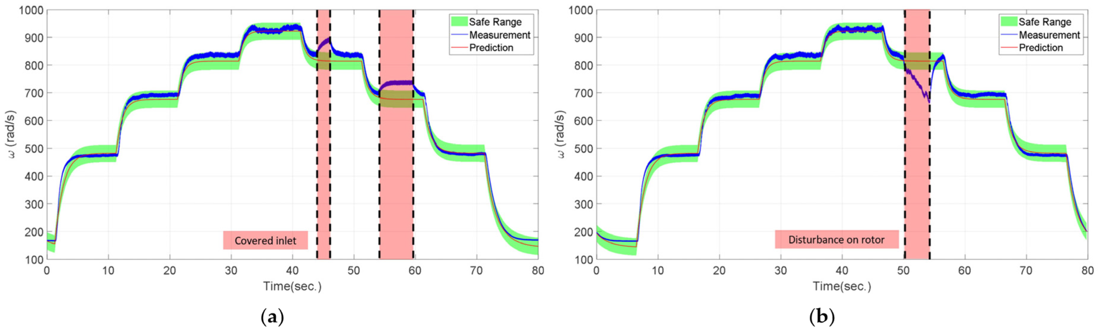
5. Anomaly Detection Result
6. Conclusions
Author Contributions
Funding
Data Availability Statement
Conflicts of Interest
References
- Guillen, D.P.; Anderson, N.; Krome, C.; Boza, R.; Griffel, L.; Zouabe, J.; Al Rashdan, A. A RELAP5-3D/LSTM model for the analysis of drywell cooling fan failure. Prog. Nucl. Energy 2020, 130, 103540. [Google Scholar] [CrossRef]
- Liu, C.; Wang, Z.; Fan, C.; Zhang, R.; Man, X. A Joint Control Strategy for Automobile Active Grille Shutter and Cooling Fan. Int. J. Automot. Technol. 2021, 22, 1675–1682. [Google Scholar] [CrossRef]
- Wiriyasart, S.; Hommalee, C.; Naphon, P. Thermal cooling enhancement of dual processors computer with thermoelectric air cooler module. Case Stud. Therm. Eng. 2019, 14, 100445. [Google Scholar] [CrossRef]
- Peng, C.-C.; Su, C.-Y. Modeling and parameter identification of a cooling fan for online monitoring. IEEE Trans. Instrum. Meas. 2021, 70, 1–14. [Google Scholar] [CrossRef]
- Peng, C.-C.; Lin, Y.-I. Dynamics modeling and parameter identification of a cooling fan system. In Proceedings of the 2018 IEEE International Conference on Advanced Manufacturing (ICAM), Yunlin, Taiwan, 16–18 November 2018; pp. 257–260. [Google Scholar]
- Schroeder, B.; Gibson, G.A. Understanding disk failure rates: What does an MTTF of 1,000,000 hours mean to you? ACM Trans. Storage (TOS) 2007, 3, 8-es. [Google Scholar] [CrossRef]
- Tao, F.; Xiao, B.; Qi, Q.; Cheng, J.; Ji, P. Digital twin modeling. J. Manuf. Syst. 2022, 64, 372–389. [Google Scholar] [CrossRef]
- Jiang, Y.; Yin, S.; Li, K.; Luo, H.; Kaynak, O. Industrial applications of digital twins. Philos. Trans. R. Soc. A 2021, 379, 20200360. [Google Scholar] [CrossRef] [PubMed]
- Colombo, A.W.; Karnouskos, S.; Kaynak, O.; Shi, Y.; Yin, S. Industrial cyberphysical systems: A backbone of the fourth industrial revolution. IEEE Ind. Electron. Mag. 2017, 11, 6–16. [Google Scholar] [CrossRef]
- Melesse, T.Y.; Di Pasquale, V.; Riemma, S. Digital twin models in industrial operations: A systematic literature review. Procedia Manuf. 2020, 42, 267–272. [Google Scholar] [CrossRef]
- Jones, D.; Snider, C.; Nassehi, A.; Yon, J.; Hicks, B. Characterising the Digital Twin: A systematic literature review. CIRP J. Manuf. Sci. Technol. 2020, 29, 36–52. [Google Scholar] [CrossRef]
- He, B.; Bai, K.-J. Digital twin-based sustainable intelligent manufacturing: A review. Adv. Manuf. 2021, 9, 1–21. [Google Scholar] [CrossRef]
- Peng, C.-C.; Chen, T.-Y. A recursive low-pass filtering method for a commercial cooling fan tray parameter online estimation with measurement noise. Measurement 2022, 205, 112193. [Google Scholar] [CrossRef]
- Prakash, N.P.S.; Chen, Z.; Horowitz, R. System identification in multi-actuator hard disk drives with colored noises using observer/Kalman filter identification (OKID) framework. arXiv 2021, arXiv:2109.12460. [Google Scholar]
- Fan, L.; Liu, X.; Cai, G.-p. Dynamic modeling and modal parameters identification of satellite with large-scale membrane antenna. Adv. Space Res. 2019, 63, 4046–4057. [Google Scholar] [CrossRef]
- Mauroy, A.; Goncalves, J. Koopman-based lifting techniques for nonlinear systems identification. IEEE Trans. Autom. Control 2019, 65, 2550–2565. [Google Scholar] [CrossRef]
- Erichson, N.B.; Brunton, S.L.; Kutz, J.N. Compressed dynamic mode decomposition for background modeling. J. Real-Time Image Process. 2019, 16, 1479–1492. [Google Scholar] [CrossRef]
- Brunton, S.L.; Proctor, J.L.; Kutz, J.N. Discovering governing equations from data by sparse identification of nonlinear dynamical systems. Proc. Natl. Acad. Sci. USA 2016, 113, 3932–3937. [Google Scholar] [CrossRef] [PubMed]
- Fukami, K.; Murata, T.; Zhang, K.; Fukagata, K. Sparse identification of nonlinear dynamics with low-dimensionalized flow representations. J. Fluid Mech. 2021, 926, A10. [Google Scholar] [CrossRef]
- Hornik, K.; Stinchcombe, M.; White, H. Multilayer feedforward networks are universal approximators. Neural Netw. 1989, 2, 359–366. [Google Scholar] [CrossRef]
- Wen, S.; Wang, Y.; Tang, Y.; Xu, Y.; Li, P.; Zhao, T. Real-time identification of power fluctuations based on LSTM recurrent neural network: A case study on Singapore power system. IEEE Trans. Ind. Inform. 2019, 15, 5266–5275. [Google Scholar] [CrossRef]
- Jiao, M.; Wang, D.; Qiu, J. A GRU-RNN based momentum optimized algorithm for SOC estimation. J. Power Sources 2020, 459, 228051. [Google Scholar] [CrossRef]
- Kim, B.-H.; Pyun, J.-Y. ECG identification for personal authentication using LSTM-based deep recurrent neural networks. Sensors 2020, 20, 3069. [Google Scholar] [CrossRef] [PubMed]
- Peng, C.-C.; Chen, Y.-H. Digital twins-based online monitoring of TFE-731 turbofan engine using Fast orthogonal search. IEEE Syst. J. 2021, 16, 3060–3071. [Google Scholar] [CrossRef]
- Peng, C.-C.; Chen, Y.-H. Modeling of a Motor-driven Propeller Dynamics System by Neural Ordinary Differential Equation. In Proceedings of the 2023 Sixth International Symposium on Computer, Consumer and Control (IS3C), Taichung, Taiwan, 3–30 July 2023; pp. 284–287. [Google Scholar]
- Chen, R.T.; Rubanova, Y.; Bettencourt, J.; Duvenaud, D.K. Neural ordinary differential equations. Adv. Neural Inf. Process. Syst. 2018, 31, 6572–6583. [Google Scholar] [CrossRef]
- Lai, Z.; Mylonas, C.; Nagarajaiah, S.; Chatzi, E. Structural identification with physics-informed neural ordinary differential equations. J. Sound Vib. 2021, 508, 116196. [Google Scholar] [CrossRef]
- Di Nunno, F.; Granata, F. Groundwater level prediction in Apulia region (Southern Italy) using NARX neural network. Environ. Res. 2020, 190, 110062. [Google Scholar] [CrossRef] [PubMed]
- Takyi-Aninakwa, P.; Wang, S.; Zhang, H.; Xiao, Y.; Fernandez, C. A NARX network optimized with an adaptive weighted square-root cubature Kalman filter for the dynamic state of charge estimation of lithium-ion batteries. J. Energy Storage 2023, 68, 107728. [Google Scholar] [CrossRef]
- Shahbaz, M.; Taqvi, S.A.A.; Inayat, M.; Inayat, A.; Sulaiman, S.A.; McKay, G.; Al-Ansari, T. Air catalytic biomass (PKS) gasification in a fixed-bed downdraft gasifier using waste bottom ash as catalyst with NARX neural network modelling. Comput. Chem. Eng. 2020, 142, 107048. [Google Scholar] [CrossRef]
- Lu, Y.; Zhong, A.; Li, Q.; Dong, B. Beyond finite layer neural networks: Bridging deep architectures and numerical differential equations. In Proceedings of the International Conference on Machine Learning, Stockholm, Sweden, 10–15 July 2018; pp. 3276–3285. [Google Scholar]


| Model Type | Parameter Estimation Method | Structure | No. of Parameters | Details |
|---|---|---|---|---|
| Physical model | Filtering integral operator | 3 | _ | |
| NARX model | Levenberg–Marquardt algorithm | 2051 | 10th order with 50 hidden states | |
| Neural ODE | ADAM optimization | 81 | 1st order with 20 hidden states | |
| Hybrid neural ODE | ADAM optimization | 34 | 1st order with 10 hidden states for NN part |
| Model Type | Training Data | Testing Data | ||||
|---|---|---|---|---|---|---|
| RMSE | Error Max | R2 | RMSE | Error Max | R2 | |
| Physical model | 3.227 | 11.563 | 0.9979 | 3.219 | 12.078 | 0.9925 |
| NARX model | 3.633 | 17.663 | 0.9973 | 6.313 | 33.009 | 0.9712 |
| Neural ODE | 3.631 | 14.169 | 0.9973 | 6.532 | 19.823 | 0.9692 |
| Hybrid neural ODE | 3.232 | 11.062 | 0.9979 | 3.194 | 11.521 | 0.9926 |
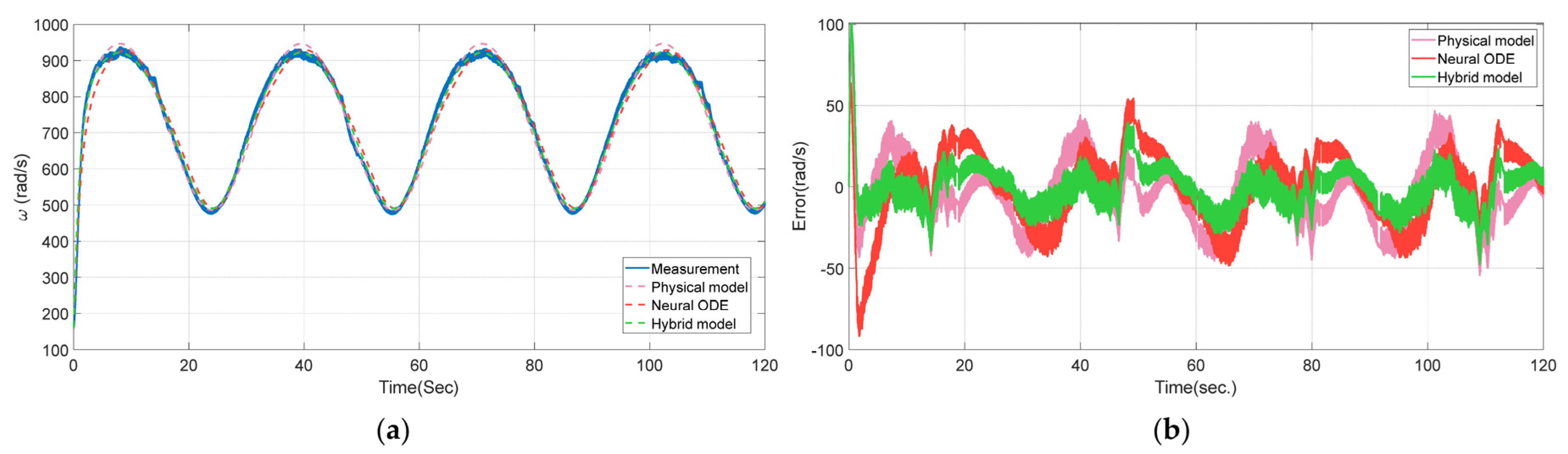
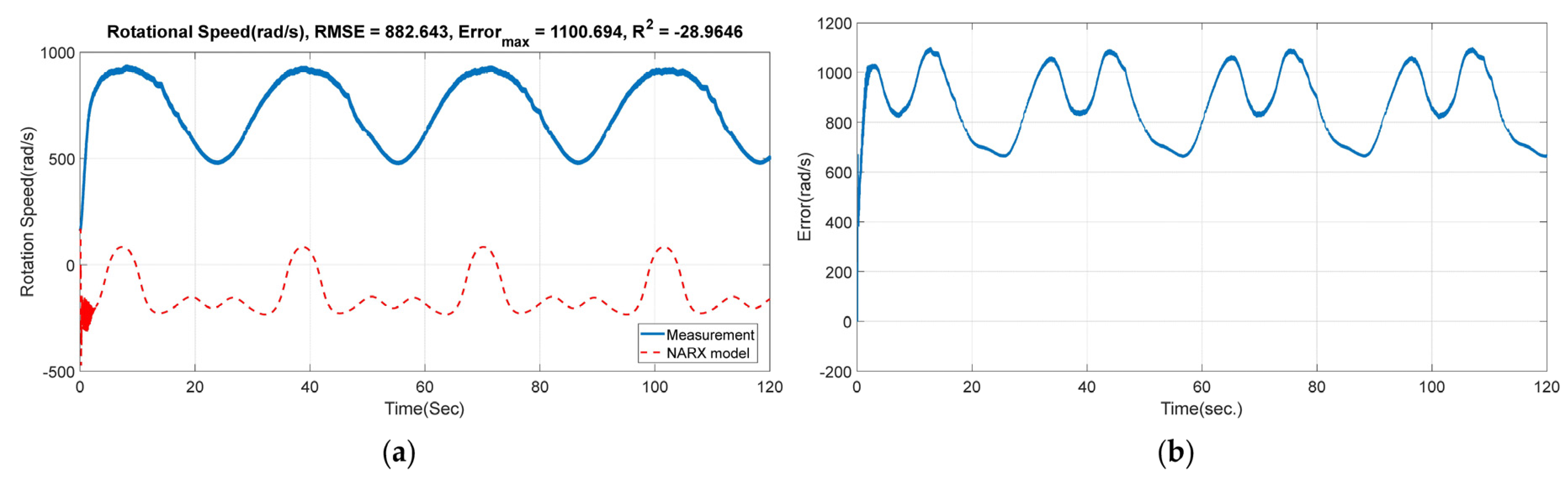
| Model Type | Training Data | Testing Data | ||||
|---|---|---|---|---|---|---|
| RMSE | Error Max | R2 | RMSE | Error Max | R2 | |
| Physical model | 35.051 | 143.455 | 0.9734 | 20.761 | 83.704 | 0.9834 |
| NARX model | 11.458 | 51.635 | 0.9972 | 882.643 | 1100.964 | −28.9646 |
| Neural ODE | 26.236 | 106.411 | 0.9851 | 23.239 | 91.775 | 0.9792 |
| Hybrid model | 17.081 | 67.99 | 0.9937 | 14.582 | 100.685 | 0.9918 |
Disclaimer/Publisher’s Note: The statements, opinions and data contained in all publications are solely those of the individual author(s) and contributor(s) and not of MDPI and/or the editor(s). MDPI and/or the editor(s) disclaim responsibility for any injury to people or property resulting from any ideas, methods, instructions or products referred to in the content. |
© 2023 by the authors. Licensee MDPI, Basel, Switzerland. This article is an open access article distributed under the terms and conditions of the Creative Commons Attribution (CC BY) license (https://creativecommons.org/licenses/by/4.0/).
Share and Cite
Peng, C.-C.; Chen, Y.-H. A Hybrid Neural Ordinary Differential Equation Based Digital Twin Modeling and Online Diagnosis for an Industrial Cooling Fan. Future Internet 2023, 15, 302. https://doi.org/10.3390/fi15090302
Peng C-C, Chen Y-H. A Hybrid Neural Ordinary Differential Equation Based Digital Twin Modeling and Online Diagnosis for an Industrial Cooling Fan. Future Internet. 2023; 15(9):302. https://doi.org/10.3390/fi15090302
Chicago/Turabian StylePeng, Chao-Chung, and Yi-Ho Chen. 2023. "A Hybrid Neural Ordinary Differential Equation Based Digital Twin Modeling and Online Diagnosis for an Industrial Cooling Fan" Future Internet 15, no. 9: 302. https://doi.org/10.3390/fi15090302
APA StylePeng, C.-C., & Chen, Y.-H. (2023). A Hybrid Neural Ordinary Differential Equation Based Digital Twin Modeling and Online Diagnosis for an Industrial Cooling Fan. Future Internet, 15(9), 302. https://doi.org/10.3390/fi15090302