A Review of ARIMA vs. Machine Learning Approaches for Time Series Forecasting in Data Driven Networks

Abstract

In the broad scientific field of time series forecasting, the ARIMA models and their variants have been widely applied for half a century now due to their mathematical simplicity and flexibility in application. However, with the recent advances in the development and efficient deployment of artificial intelligence models and techniques, the view is rapidly changing, with a shift towards machine and deep learning approaches becoming apparent, even without a complete evaluation of the superiority of the new approach over the classic statistical algorithms. Our work constitutes an extensive review of the published scientific literature regarding the comparison of ARIMA and machine learning algorithms applied to time series forecasting problems, as well as the combination of these two approaches in hybrid statistical-AI models in a wide variety of data applications (finance, health, weather, utilities, and network traffic prediction). Our review has shown that the AI algorithms display better prediction performance in most applications, with a few notable exceptions analyzed in our Discussion and Conclusions sections, while the hybrid statistical-AI models steadily outperform their individual parts, utilizing the best algorithmic features of both worlds.

1. Introduction

In the context of academic bibliography, the tools and methods of Machine and Deep Learning constitute an alternative approach to statistical methods for time series forecasting. However, the available data with regard to their relative performance in terms of accuracy and computational demands is limited [1]. Artificial Intelligence, which is a superset of machine and deep learning, has expanded during the last decade in multiple fields of entrepreneurial and academic activity, with applications regarding the financial sector, medical care, industry, retail, supply chain, utilities, and networks [2]. Nevertheless, the classical approach with respect to the analysis and forecasting of time series is mostly based on integrated autoregressive moving average (ARIMA) models, and their various versions [3]. Moreover, a core issue of the existing academic literature in the field of machine learning forecasting techniques is the fact that the majority of publications point to adequate accuracy values, without a proper foundation, meaning without a preestablished comparison with the results of simple statistical methods and prediction models [1].

In the present study, we will attempt a review of ARIMA, Machine Learning, and Deep Learning techniques with regard to their relative performance in time series forecasting. The strategy behind our review is to present a selection of academic papers in which the performance of machine learning, deep learning, and hybrid prediction models is compared with the performance of the ARIMA or SARIMA (Seasonal ARIMA) algorithms based on a variety of metrics. The results of these studies are presented in Table 2, Table 3, Table 4 and Table 5. The scientific works presented in this review consist of research in the financial sector (with a special focus on the application of bitcoin price prediction), in the health sector (with a special focus on the applications of predicting parameters and variables related to the disease of COVID-19), in the field of weather forecasting (wind speed, drought, solar energy production, etc.), in the field of utility parameters forecasting (offer and demand of energy, water consumption, oil production, etc.), and in network parameters prediction (both transportation and web network traffic prediction).

1.1. Data Driven Networks

The title of the present work refers to “data driven networks”, from the point of view of data and models used in time series forecasting. Big data collection is of utmost importance to modern forecasting applications, especially for the training of efficient machine learning predictive models, due to the fact that the problem of forecasting increases in complexity as the volume and dimensionality of available data sources increase. In recent applications and study fields regarding time series forecasting, the collection of data relies on large-scale networks of sensors and data collection points due to the distributed nature of the target applications. The analysis and forecasts based on these datasets are also fed to large-scale network applications (e.g., large-scale weather forecasts, health strategy planning on a national and global level, sales management on a global scale, etc.).

On the other hand, the term “data driven networks” also refers to the training and efficient deployment of the models proposed for time series forecasting by the scientific community. Especially in the case of machine learning models, whose application is mostly data- and problem-agnostic, data availability in sufficient quantity is crucial to successful forecasting.

1.2. Scientific Contributions

The present work attempts to address the existing gap in the scientific literature, regarding an extensive summary/review of the studies comparing the application of ARIMA and machine learning techniques in time series forecasting applications. This is the only such review, according to the authors’ best knowledge.

Our work compares time series forecasting studies across multiple applications and data sources, and it consists of mostly recent comparative studies published after 2018 (with the exception of the works of Zhang et al. [4] and Nie et al. [5]). Due to the multitude of different data sources and forecasting challenges, we attempt a multilateral, sampled view of the existing literature, presenting studies from five basic data categories (financial, medical, weather, utilities, and network characteristics). For the above reasons, our work constitutes a contemporary, multifaced, review of the existing literature comparing the ARIMA statistical approach with its machine learning counterparts. Our study also summarizes the main performance metrics of the algorithms presented in each study, thus enabling an intuitive review and comparison of the methods in each forecasting application. A practical evaluation (Section 5) of the studies in which the ARIMA models outperform their machine learning counterparts results in an enumeration of the application, dataset, and model-dependent characteristics that drive the choice of the optimal forecasting model in any particular application.

1.3. Rationale and Structure

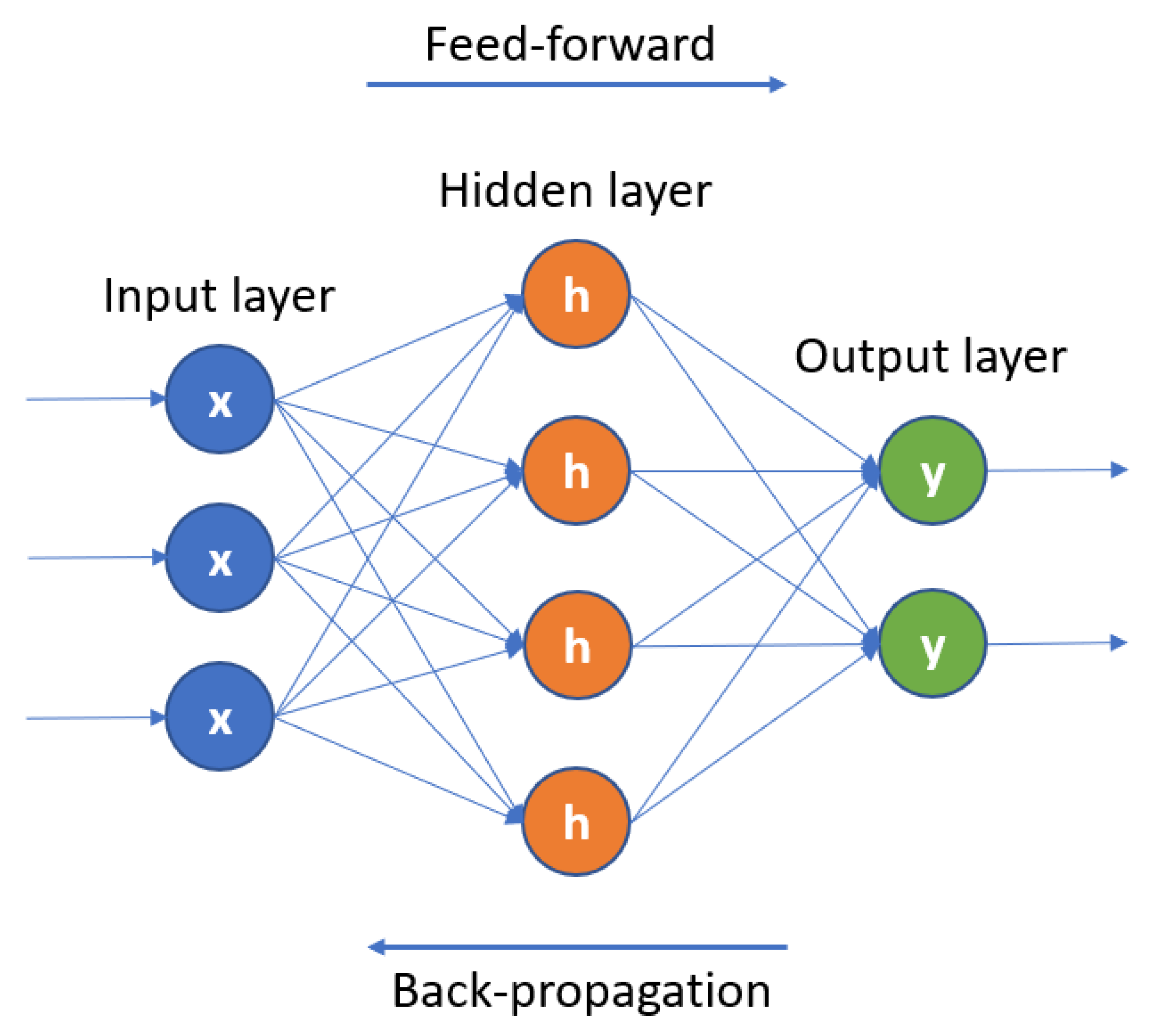
The rationale behind the structure of our review is based on organizing the collected scientific literature first in relation to the machine learning model being compared with ARIMA and second in relation to the field of forecasting applications. In that scope, the first model category to be presented in detail is ARIMA, which is the center of our review, and then we organize the machine learning approaches by model category. For each of the categories, we present the theoretical background, and then we demonstrate the relevant scientific literature organized by application category. The same principle applies to the category of hybrid forecasting models, meaning the combination of ARIMA and machine learning algorithms. Finally, we evaluate the reviewed scientific literature in total, and based on the finding that machine learning models outperform the ARIMA approach in the majority of forecasting applications, we aim to uncover the conditions under which we have a superior ARIMA forecasting result.

At this point, it is important to note that our work does not propose a new time series forecasting model, but rather constitutes an organized review of the published scientific literature comparing the ARIMA approach to different machine learning, and hybrid prediction models. We consider this aspect of our work crucial to the feasibility of our study because we aim to compare the optimized ARIMA and machine learning models on the same datasets. Therefore, although the scientific literature applying individual ARIMA or machine learning models to forecasting problems is extensive, we base our study only on the explicit comparisons of the three categories of models (ARIMA, machine learning, and hybrid).

The present work is organized as follows: The problem of time series forecasting, which—along with the ARIMA technique—constitutes the center of our work, is presented in Section 2, along with the morphological characteristics of the time series that affect the choice of the forecasting algorithm and their respective results. A review is also carried out regarding the time series data sources and their inherent characteristics that predetermine the format of the data to be analyzed and, consequently, the choice of the forecasting algorithms. In Section 3 and Section 4, we perform a theoretical review of the algorithms and machine learning models that will be presented in the context of the attempted comparisons, and subsequently, we present the relevant scientific literature, organized by field of research (financial sector, medical care, etc.). 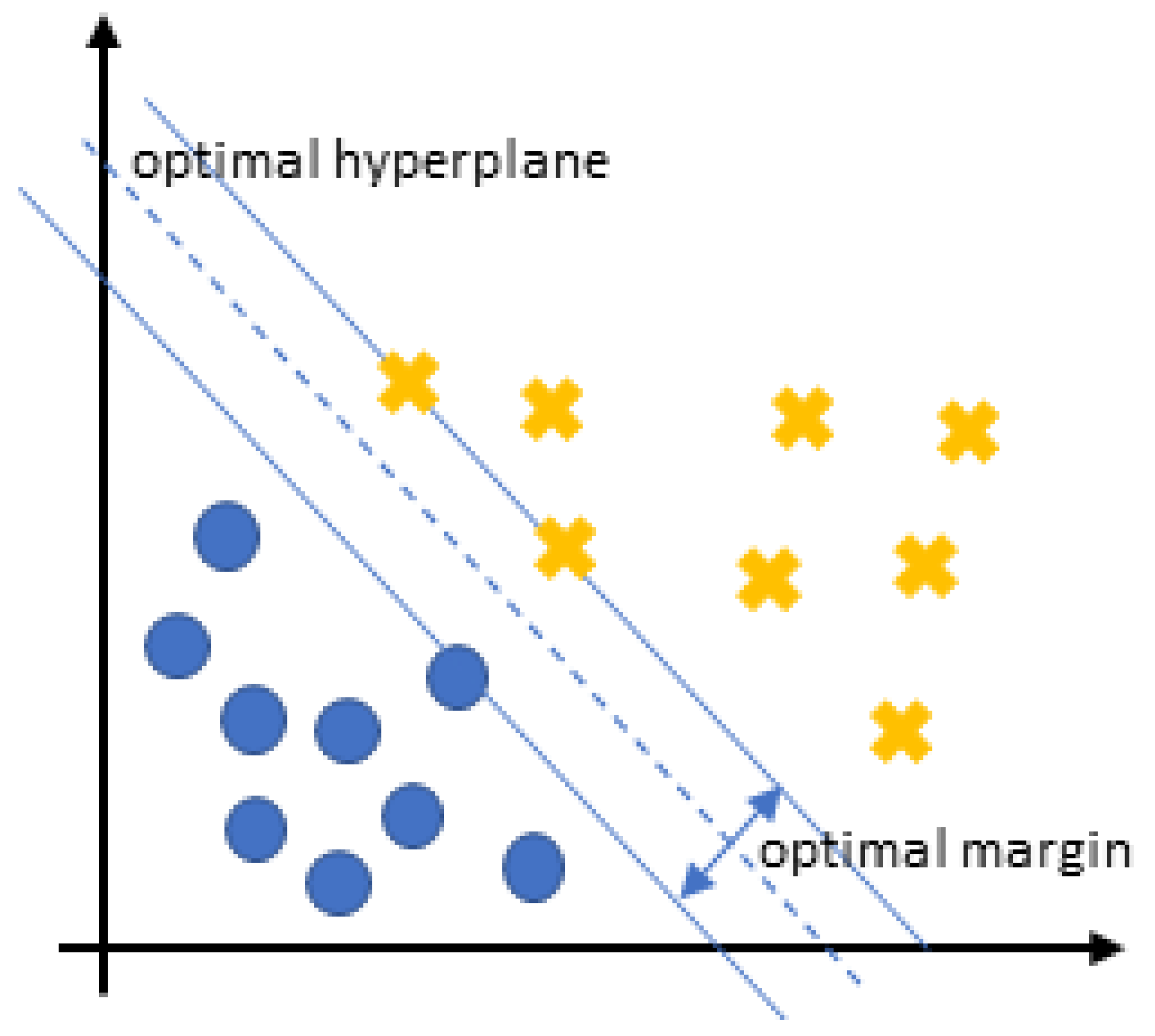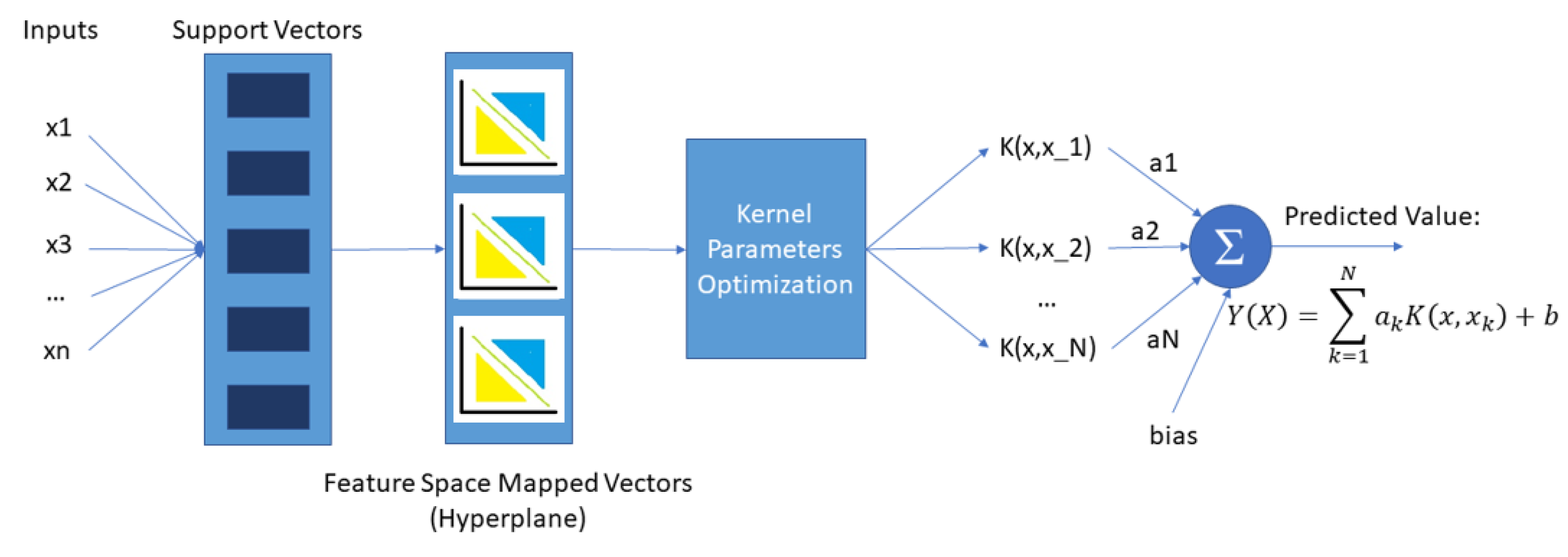Specifically, in Section 3.1, we refer to the comparison of the SVM model with the classic ARIMA statistical technique, while in Section 3.2, the theory and applications of decision tree-based models are analyzed. Section 4 presents the rationale behind the development of hybrid forecasting models with a review of the indicative scientific literature. In any case, the hybrid models chosen for presentation and analysis are a combination of the ARIMA technique with a specific machine learning model. Section 5 constitutes a practical evaluation of the reviewed literature, with a focus on extracting the conditions under which the ARIMA approach exhibits superior predictive performance compared with the machine learning models. Finally, Section 6 covers the conclusions of our review.

2. Background: Data and Autoregressive Models

2.1. Time Series Data: Forecasting

Time is the central characteristic that distinguishes time series from other types of data. This property of theirs is both a limitation and a structural element of the data collection, as well as a source of additional information for their analysis [6]. Essentially, time series data is any type of information presented as an ordered sequence and can be defined as a collection of observations of some variable, organized into equally spaced time intervals [7].

The question of forecasting is one of the most difficult and essential problems that time series analysis must deal with. The performance and accuracy of the analysis results vary depending on the type of data and its assumptions. In addition to these parameters, the analysis is also affected by factors inherent to the respective field of research, such as the periodicity of the time series, unforeseen events, changes in the structure of the organizations or structures from which the data are collected, etc. [8]. The “No-Free-Lunch” theorem proves that it is not possible to have a forecasting method that gives optimal performance for all possible time series [9]. There is a significant amount of research literature on predictive models, and the results of these studies indicate the existence of two macro-categories of methods: statistical methods and machine learning methods. In the continuation of our paper, we will refer to the following categories of time series forecasting models: (a) statistical models, (b) machine and deep learning and (c) hybrid models [10].

The comparison of the forecasting results of the aforementioned models in the context of the studies presented in the present work is based on various metrics, figure of merits, whose mathematical formulas are expressed below, where $y_t$ is the real value of the series at the time point t, $\widehat{y_t}$ is the corresponding forecasted value given by the model, and N is the time period of the forecast:

• Mean Squared Error (MSE)

$$MSE=\frac{1}{N}\sum _{t=1}^N{(y_t-\widehat{y_t})}^2.$$

(1)

The popular error metric RMSE is used in the scientific literature in place of MSE (same scale of the variable), and it is the square root of the MSE metric.

• Mean Absolute Percentage Error (MAPE)

$$MAPE=\frac{1}{N}\sum _{t=1}^N|\frac{y_t-\widehat{y_t}}{y_t}|.$$

(2)

• =Mean Absolute Error (MAE)

$$MAE=\frac{1}{N}\sum _{t=1}^N|y_t-\widehat{y_t}|.$$

(3)

• Coefficient of determination ($R^2$)

It is a statistical measure to indicate the proportion of the dependent variable variation in a model that can be predicted from the variation in the independent model variables, and it is a metric used to determine how well our model fits a set of observations.

• Mean Absolute Deviation (MAD)

$$MAD=\frac{1}{N}\sum _{t=1}^N\left|\right(y_t-m\left(Y\right)|,$$

(4)

where $m\left(X\right)$ is the mean value of the forecasted values for the specific time range.

• Nash–Sutcliffe model efficiency coefficient (NSE)

It is a metric used to assess the predictive capacity of hydrological models. It is computed using the following mathematical formula:

$$NSE=1-\frac{{\sum }_{t=1}^N{(Y_o^t-Y_m^t)}^2}{{\sum }_{t=1}^N{(Y_o^t-\overline{Y_o})}^2},$$

(5)

where $\overline{Y_o}$ is the mean of observed discharges, $Y_m$ is the modeled discharge and $Y_o^t$ is the observed discharge at time t.

• Kolmogorov-Smirnov test (K-S distance)

The Kolmogorov–Smirnov test quantifies a distance metric between the distribution of our model outputs and a reference distribution defined by the null hypothesis of our study.

• Normalized Mean Absolute Error (NMAE)

This metric is used specifically in the energy forecasting domain, being able to generalize under different upper bounding conditions.

$$NMAE(\%)=\frac{1}{N}\sum _{t=1}^N\frac{|y_t-\widehat{y_t}|}{C}\times 100,$$

(6)

where C is the capacity of the power plant.

2.2. Time Series Data: Characteristics

Data derived from time series may have the following characteristics [6]:

• Trend: This characteristic is associated with the presence of an upward, downward, or stable course of the series, with respect to the time dimension.
• Seasonality: This characteristic indicates the existence of periodic patterns in the behavior of the time series, which repeat with a fixed frequency.
• Stationarity: Stationary is a time series whose statistical properties (average, variance, dispersion of values, etc.) are stable over time. A stationary time series with no trend implies that its fluctuations around its mean have a constant width. Furthermore, the autocorrelation of static time series remains constant over time. Based on these assumptions, a time series of this form can be thought of as a combination of signal and noise [11].

In addition to these basic characteristics, some of the more common patterns seen in time series data are the following [7]:

-Cyclic behavior: In contrast to seasonal patterns, cyclical patterns appear when the factors influencing the data of each time series are not distinguished by a fixed or known frequency. This particular pattern mainly concerns studies related to financial data, where cyclical behavior is observed according to the cycles of the economy and the business environment. The average duration of these cycles is usually longer than the duration of seasonal patterns, of the order of two years.

-Diurnality: Refers to the inherent patterns observed in time series originating from a particular application that have a daily or monthly repeat cycle. Data related to solar, or weather observations are some examples indicating this property.

-Outliers: Regarding the detection of anomalies and outliers in time series data, the analysis focuses on identifying abnormal changes, both desirable and undesirable, in the data set.

-White noise: This characteristic refers to the cases where the data does not follow a specific pattern.

2.3. Time Series Data Sources

Time series data can come from a multitude of sources and systems with different classes of characteristics, complexity, volume, and frequency of acquisition. Some categories of sources of this kind of data are industrial production, the financial sector, the consumer electronics industry, health system structures, retail trade, meteorology, and generally any measurable and quantifiable manifestation of human life and its environment. Especially in recent years, through the exponential growth of data sources, time series analysis and forecasting systems have been required to approach models of ever-increasing dimension and complexity.

Time series from complex systems capture the dynamic behavior and causes of the underlying processes and provide a practical means of predicting and monitoring the evolution of the system state. However, the non-linearity and non-stationarity that often characterize the underlying processes of these systems pose a strong challenge to the process of accurate prediction. For most real-world systems, their dynamical state vector field is a nonlinear function of the state variables, meaning that the relationship connecting the system’s intrinsic state variables to their autoregressive terms and exogenous variables is nonlinear. The time series resulting from such complex systems show aperiodic (chaotic) patterns even in steady states. Furthermore, since real-world systems often evolve under transient conditions, the signals obtained from them tend to exhibit various forms of non-stationarity. However, the methods that dominate the literature on the analysis and forecasting of time series derived from such systems focus mainly on the forecasting of linear and static processes. According to the work of Cheng et al. [12], conventional forecasting approaches, such as ARIMA techniques, cannot adequately capture the evolution of these systems from the perspectives of forecasting accuracy, computational workload, and sensitivity to the quantity and quality of a priori input information. This finding prompts us to assume that the success of the used prediction method, both in the category of classical algorithms and in the category of machine learning and deep learning techniques, depends to a large extent on the complexity of the system described by the data. From this point of view, artificial intelligence has an advantage over ARIMA techniques, as will be seen from the results of the studies presented later in the paper. At this point, it must be mentioned that a number of non-linear transformations exist for optimizing the ARIMA models in non-linear forecasting applications, which we will refer to in the ARIMA theoretical background of our study. On this note, there are a few notable exceptions where the performance of classical techniques exceeds that of artificial intelligence methods. These results will be commented on in the conclusions of our research.

2.4. AutoRegressive Integrated Moving Average (ARIMA) Models

The ARIMA model is a generalization of the ARMA model (AutoRegressive Moving Average model), suitable for handling non-stationary time series. As the classical ARMA model takes for granted the stationarity of the time series it is asked to analyze, the management of inherently non-stationary time series requires their transformation into a static data series by eliminating seasonality and trends, through a finite-point differentiation [3]. As mentioned earlier, a stationary time series can be thought of as a combination of signal and noise. The ARIMA model handles the time signal, after first separating it from the noise, and outputs its prediction for a subsequent time point [11]. As indicated by the method’s acronym, its structural components are the following [13]:

• AR: Autoregression. A regression model that uses the dependence relationship between an observation and a number of lagged observations (model parameter p).
• I: Integration. Calculating the differences between observations at different time points (model parameter d), aiming to make the time series stationary.
• MA: Moving Average. This approach considers the dependence that may exist between observations and the error terms created when a moving average model is used on observations that have a time lag (model parameter q).

The AR model of order p, AR(p), can be written as a linear process as follows:

$$x_t=c+\sum _{i=1}^p{\varphi }_i{x}_{t-i}+{ϵ}_t,$$

(7)

where $x_t$ the static variable, c a constant, the terms ${\varphi }_i$ are autocorrelation coefficients at the time delay steps $1,2,\dots ,p$ and ${ϵ}_t$ are the samples of the Gaussian white noise series, with zero mean and ${\sigma }^2$ variance.

A simple moving average model of order q, MA(q), can be given as:

$$x_t=\mu +\sum _{i=0}^q{\theta }_i{ϵ}_{t-i},$$

(8)

where $\mu$, is the expected value of $x_t$ (it mostly equals to 0), ${\theta }_i$ the weights applied to the current and past values of the stochastic term of the time series, and ${\theta }_0=1$. We consider ${ϵ}_t$ to be a Gaussian white noise series, with zero mean and ${\sigma }_{ϵ}^2$ variance.

By combining these two models, autoregression and moving average, we create the ARMA model of class (p,q):

$$x_t=c+\sum _{i=1}^p{\varphi }_i{x}_{t-i}+{ϵ}_t+\sum _{i=0}^q{\theta }_i{ϵ}_{t-i},$$

(9)

where ${\varphi }_i\ne 0,{\theta }_i\ne 0,{\sigma }_{ϵ}^2>0.$ The parameters p, q constitute the order of the AR and MA models respectively.

The general form of an ARIMA model is written as ARIMA(p, d, q), including the integration term that guarantees the stationarity of the time series [13], and it can be expressed as:

$${\nabla }^d{x}_t=c+\sum _{i=1}^p{\varphi }_i{\nabla }^d{x}_{t-i}+\sum _{i=0}^q{\theta }_i{ϵ}_{t-i},$$

(10)

where ${\nabla }^d$ is a differential factor, introducing a difference of order d, aiming to remove the nonstationarity of the time series $x_t$ [14].

Table 1. Nonseasonal ARIMA models for time series forecasting. Random-walk and random-trend, autoregressive and exponential smoothing models constitute specific cases of the general ARIMA models. The additional presence of a constant in the models, accounts for any underlying trend or mean in the data, in order to improve their predictions and overall performance in the forecasting tasks.

Forecasting Equation	ARIMA(p,d,q)
first-order autoregressive model	ARIMA(1,0,0)
random walk	ARIMA(0,1,0)
differenced first-order autoregressive model	ARIMA(1,1,0)
simple exponential smoothing	ARIMA(0,1,1)
simple exponential smoothing with growth	ARIMA(0,1,1)
linear exponential smoothing	ARIMA(0,2,1)
linear exponential smoothing	ARIMA(0,2,2)
damped-trend linear exponential smoothing	ARIMA(1,1,2)

displays the basic parameter combinations for the nonseasonal ARIMA models.

2.4.1. ARIMA Parameter Determination

The optimal selection of the ARIMA p, d, and q parameters is crucial to the success of the forecasting procedure. The combination of the p and q parameters is based on the examination of the autocorrelation function (ACF) and partial autocorrelation function (PACF) plots for the specific dataset, while the d parameter is chosen in order to stationarize the time series.

In most of the scientific literature presented in the rest of this work, it is often needed to identify the best-performing ARIMA model among a number of different ARIMA (p,d,q) models for a specific forecasting application. In these cases, the selection criteria include the Akaike (AIC) and Bayesian (BIC) information criteria. The AIC measures the quality of a forecasting model, keeping a balance between overfitting and model complexity. In the case of BIC, the same rule applies, but with a higher penalty for complex models. In both criteria, lower values signify a better model.

There have been many attempts to automate the selection of the ARIMA model parameters over the years, using different tests in order to determine the optimal values for both seasonal and non-seasonal models. The auto.arima function in R [15] constitutes a popular heuristic method for parameter selection in an ARIMA application, and it is based on a simple step-wise algorithm:

1. Start with a small number of basic ARIMA models and select the one with the minimum AIC value.

2. Consider up to a number of variations of the selected model and calculate the AIC value for each one. Whenever a model with a lower AIC is found, it replaces the reference model, and the procedure is repeated. The algorithm finishes when we cannot find a model close to the reference model with a lower AIC value.

A valid ARIMA model is always returned by the above algorithm due to the fact that the model space is finite and that at least one of the starting models will be accepted as a solution [16].

2.4.2. ARIMA Variants

In cases of seasonal time series, it is possible, during the analysis, for the forecasting model to be partially shaped by non-seasonal, short-duration features of the data. Consequently, the formulation of a seasonal ARIMA model is required, which incorporates seasonal and non-seasonal factors into a combined model. The general form of a seasonal ARIMA model is represented by the formula: $ARIMA(p,d,q)x{(P,D,Q)}_S$ where p is the non-seasonal AR order, d is the non-seasonal differencing order, q is the non-seasonal MA order, P is the seasonal AR order, D is the seasonal differencing order, Q is the seasonal MA order and S is the recurrence time range of the seasonal pattern. The most important step in calculating a seasonal ARIMA model is determining the values of the parameters (p, d, q) and (P, D, Q).

The ARIMA technique has evolved over the years, resulting in the development of many variants of this model, such as the SARIMA (Seasonal ARIMA) and ARIMAX (ARIMA with Explanatory Variable) techniques. These models perform well in terms of short-term forecasts, but their performance is severely degraded for long-term predictions [8].

2.4.3. Advantages and Disadvantages

The ARIMA technique presents several advantages, among which are the use of an online learning environment, the independence between sample size and storage costs, as well as the fact that parameter estimation can be performed online, in an efficient and scalable way. The disadvantages of this technique are the subjectivity of its progress evaluation, the fact that the reliability of the selected model may depend on the skill and experience of the specific forecaster, and the existence of several limitations to the parameters and classes of possible models. A consequence of all these limitations is the fact that the final choice of the prediction model can be a difficult task [17].

Another important aspect of the application of the ARIMA to time series forecasting is the linearity of the dataset it aims to predict. The basic form of the ARIMA algorithms is designed to handle linear data relationships. However, their scope of successful application in forecasting can be significantly extended, considering the various transformations available, which extend the method’s capability to handle non-linear time series. A widely used family of such transformations, including both logarithmic and power transformations, is the Box-Cox toolset [18], depending on the $\lambda$ parameter and defined as:

$$w_t=\left\{\begin{array}{c}log\left(y_t\right)if\lambda =0\hfill \\ \frac{y_t^{\lambda }-1}{\lambda }otherwise\hfill \end{array}\right..$$

(11)

Based on the value of $\lambda$, the new time series can be transformed in order to improve the forecasting model.

3. Machine Learning Models

In the present work, the field of machine learning is regarded as a subset of the field of artificial intelligence, and a superset of the field of deep learning methods. In that scope, we present the SVM and Decision Tree-based approaches to the problem of time series forecasting for the machine learning family of methods and the basic deep learning models that are used by the publications presented in the rest of the study. The models we selected to present do not form an exhaustive list of machine learning techniques; rather, they represent some of the main algorithmic categories used in the recent scientific literature for benchmarking the ARIMA models against machine learning techniques.

3.1. Support Vector Machines (SVM)

It is a supervised learning technique in the field of machine learning used for data classification. The goal of SVMs is to find an appropriate, for each classification problem, hyper layer partition of the data space (Figure 1), with the aim of correctly classifying the data while achieving the maximum possible classification margin [19]. This hyperplane maximizes a distance metric between classification classes. The classification of the data is completed in two steps: In the first step, the support vector machine is fed with a set of data and their labels, i.e., the information about the class to which each one belongs. During this step, the algorithms iteratively optimize some mathematical criterion based on the labeled data. The training data that constrain the maximum allowable margin between classes constitute the support vectors [11]. In Figure 2, the sequence of the SVM processing steps is depicted graphically.

In the field of time series forecasting, the regression variant of the SVM model (support vector regression (SVR)) is used in the scientific literature with increasing frequency. The difference between this particular methodology and the traditional time series forecasting algorithms is its data-driven approach to the forecasting problem, in contrast to the model-driven classical approach. In training the appropriate SVR model for time series prediction, the independent variables utilized in the scientific literature are the lags of the dependent variable x of the specific forecasting problem. The SVR model is optimized for a varying number of lags based on a specified error metric.

Table 2. Summary of ARIMA and SVM Comparison Studies in Time Series Forecasting. In the works of Singh et al. and Zhang et al. the ARIMA parameters were optimized for each observation site.

Article	Algorithms	Metrics	Dataset
Makala et al. [20]	ARIMA$(2,1,2)\times {(2,1,2)}_{12}$	RMSE	gold price
	SVM	MAPE
Singh et al. [21]	SVM	MAE	COVID-19 confirmed cases
		MSE
		RMSE
Atique et al. [22]	ARIMA$(0,1,2)\times {(1,0,1)}_{30}$	MAPE	solar energy generation
	SVM
	ANN
Tiwari et al. [23]	ARIMA${(0,1,12)}_{day}$	MSE	ambient noise levels
	ARIMA${(0,1,10)}_{night}$	RMSE
	SVM	MAPE
		$R^2$
Zhang et al. [24]	ARIMA	$R^2$	drought forecasting
	WNN	MSE
	SVM	NSE
		K-S distance
Al Amin et al. [25]	ARIMA$(2,1,1)$	MAPE	short time load forecasting
	SVM (for non-linear	MSE
	load pattern)
Liu et al. [26]	ARIMA	various	urban water consumption
	BP
	SVM

Table 2. Summary of ARIMA and SVM Comparison Studies in Time Series Forecasting. In the works of Singh et al. and Zhang et al. the ARIMA parameters were optimized for each observation site.

Article	Algorithms	Metrics	Dataset
Makala et al. [20]	ARIMA$(2,1,2)\times {(2,1,2)}_{12}$	RMSE	gold price
	SVM	MAPE
Singh et al. [21]	SVM	MAE	COVID-19 confirmed cases
		MSE
		RMSE
Atique et al. [22]	ARIMA$(0,1,2)\times {(1,0,1)}_{30}$	MAPE	solar energy generation
	SVM
	ANN
Tiwari et al. [23]	ARIMA${(0,1,12)}_{day}$	MSE	ambient noise levels
	ARIMA${(0,1,10)}_{night}$	RMSE
	SVM	MAPE
		$R^2$
Zhang et al. [24]	ARIMA	$R^2$	drought forecasting
	WNN	MSE
	SVM	NSE
		K-S distance
Al Amin et al. [25]	ARIMA$(2,1,1)$	MAPE	short time load forecasting
	SVM (for non-linear	MSE
	load pattern)
Liu et al. [26]	ARIMA	various	urban water consumption
	BP
	SVM

3.1.1. Financial Data

In the scientific literature related to time series forecasting applications, SVM and ARIMA techniques are contrasted in analyzing data from a wide variety of sources (Table 1). In the economic domain, the work of Makala et al. [20] compared the capabilities of classical ARIMA and SVMs in predicting the daily price of gold. The results of the study show that the prediction using SVMs outperforms ARIMA based on the root mean square error (RMSE) and mean absolute percentage error (MAPE) metrics, with RMSE = 0.028 and MAPE = 2.5 for SVM and RMSE = 36.18 and MAPE = 2897 for ARIMA, respectively. This particular research also supports the popularization of the use of SVM techniques in the price prediction of any product due to the accuracy of their results.

3.1.2. Healthcare Data

Regarding the field of medical care, in the work of Singh et al. [21], least-squares ARIMA and SVM models are applied to data on the daily confirmed cases of SARS-CoV-2 in the five countries with the highest number of cases during the time period of publication of this paper (Italy, Spain, France, United Kingdom, and the USA), with the aim of predicting the number of confirmed cases over a period of one month in these countries. The ARIMA parameters were optimized separately for each country. According to the conclusions of this paper, ARIMA and Least Squares SVM models have different handling approaches for data coming from different countries: the research results indicate a drop in errors (MAE, MSE, and RMSE) and an increase in prediction accuracy (coefficient determination) using the least squares SVM model, with a percentage difference of 80% in the prediction of the number of confirmed cases for Spain with respect to the ARIMA technique and a difference of 60% for the predictions concerning Italy and France.

3.1.3. Energy and Noise Prediction

The superiority of SVM models for time series forecasting in relation to the classical statistical approach of ARIMA is also indicated by the results of the work of Atique et al. [22], regarding the prediction of the solar energy collected by a solar panel during a calendar year. This work also highlights the need to improve the overall prediction accuracy of the models. In the same direction, the study of Tiwari et al. [23] focuses on time series modeling using conventional SVM and ARIMA techniques on 3 years of noise time series data, from January 2015 to December 2017. The study compared the performance of the radial basis function SVM model with the ARIMA model, resulting in the superiority of the SVM model over the ARIMA model in terms of margin of error and adaptability to data non-linearity.

3.1.4. Weather

In a different field of research, the work of Zhang et al. [24] investigated and compared the prediction abilities of ARIMA, Wavelet Neural Network (WNN), and SVM models for drought time series in the Sanjiang Plain in China. The models of this research were based on the prediction of SPEI (standard precipitation evapotranspiration index) values collected during the period 1979–2016 from seven meteorological stations in the study area. For each of the sites, the parameters of the seasonal ARIMA model were optimized using Akaike’s Information Criterion (AIC). The comparison between the raw data values and the predictions resulted in the following $R^2$ and NSE (Nash-Sutcliffe coefficient of performance) values: 0.837 and 0.831 for the WNN network, 0.833 and 0.827 for the SVM network, while the corresponding values of the classical ARIMA algorithms were above 0.9. In addition, the ARIMA models had smaller MSE values and better overall performance than the other two models, while the analysis of variance showed that the ARIMA models had a clear advantage over the other two models in predicting the drought in the Sanjiang Plain in China based on various performance indicators (R2, MSE, NSE, and Kolmogorov-Smirnov distance). According to the results of the study, WNN and SVM machine learning models do not necessarily perform better than traditional ARIMA models in drought prediction. Different methods can be used to analyze data from different regions, and the characteristics of the data should be carefully analyzed in order to select the appropriate prediction model.

3.1.5. Utilities

The research of Al Amin et al. [25] on power grid load forecasting concludes that the SVM model can predict the energy consumption profile pattern and achieve higher accuracy than ARIMA models. However, SVM failed to predict the magnitude of consumption peaks in some cases, which is related to unpredictable changes in consumer behavior. The comparison of the two models also highlights the fact that SVM performs better in the case of non-linear consumption patterns, while ARIMA exhibits better behavior in the linear load approximation. Finally, in the work of Liu et al. [26], ARIMA, Back-Propagation Neural Network, SVM, and hybrid EEMD-ARIMA, EEMD-BP, and EEMD-SVM (ensemble empirical mode decomposition) models were compared in predicting hourly water consumption in Shanghai city in China. This work shows that the SVM model outperforms the ARIMA and that the hybrid EEMD-SVM model has the best performance (based on various metrics), while it appears that the use of EEMD decomposition improves the prediction accuracy of the algorithms. The research also concludes that the optimal length of the training time series for hybrid algorithms is over one week.

3.2. Decision Trees and Random Forests

Another major category of machine learning algorithms applied to the problem of time series forecasting is the set of tree-based models. This category, although underrepresented in the scientific literature in comparison to its deep learning counterparts, is at the forefront of many recent forecasting competitions’ leaderboards [27].

In time series forecasting, decision trees form a succession of binary decisions associated to supervised features of the used dataset, which drive the forecasting procedure based on the minimization of the data variance [28]. The modeling of the decision tree for time series is based on the classification and regression tree algorithm (CART), developed by Breiman et al. [29].

Random forests are formed by aggregating the decisions of a number of trees on a specific problem. In time series forecasting, the use of random forest regression algorithms has the advantage of a lower model variance in relation to other machine learning approaches [30]. Two of the most prominent models that also display superior performance in forecasting competitions are XGBoost and Lightgbm. XGBoost constitutes an implementation of the Gradient Boosting learning method, namely that it combines a number of weak learners into a strong learner in a linear fashion. Both CART and linear classifiers can be used as base models for the XGBoost algorithm, while a second-order Taylor expansion of the cost function entails an enhanced information profile. The Lightgbm model is another implementation of the Gradient Boosting Decision Tree algorithm (GBDT), based on two novel techniques: gradient-based one-side sampling and the exclusive feature bundling [31].

In the scientific literature presented in later sections of this work, the XGBoost algorithm appears in comparison to ARIMA and deep learning models in the work by Paliari et al. [32]. In this paragraph, we will present some comparative results derived from the popular Makridakis forecasting competitions, as well as from the recently published scientific literature.

Table 3. Summary of ARIMA and Decision Tree-based models’ Comparison Studies in Time Series Forecasting.

Article	Algorithms	Metrics	Dataset
Alim et al. [33]	ARIMA$(0,1,1)\times {(0,1,1)}_{12}$	MAE	infectious disease prediction
	XGBoost	RMSE
		MAPE
Lv et al. [34]	ARIMA$(3,1,0)\times {(1,1,0)}_{12}$	MAE	infectious disease prediction
	XGBoost	MPE
		MAPE
		RMSE
		MASE
Fang et al. [35]	ARIMA$(0,1,1)\times {(0,1,1)}_7$	MAE	COVID-19 confirmed cases
	XGBoost	RMSE
		MAPE
Noorunnahar et al. [36]	ARIMA$(0,1,1)$	MAE	annual rice production
	XGBoost	MPE
		RMSE
		MAPE
Zhang et al. [37]	ARIMA	RMSE	retail sales volume
	LSTM	MAE
	Prophet
	GBDT
	XGBoost
Priyadarshini et al. [38]	ARIMA$(2,1,1)$	MSE	short time load forecasting
	SARIMA	RMSE
	LSTM	MAE
	LightGBM
	Prophet
	VAR
Makridakis et al. [39]	various	various	retail unit sales (M5)
			multiple categories (M4)

Table 3. Summary of ARIMA and Decision Tree-based models’ Comparison Studies in Time Series Forecasting.

Article	Algorithms	Metrics	Dataset
Alim et al. [33]	ARIMA$(0,1,1)\times {(0,1,1)}_{12}$	MAE	infectious disease prediction
	XGBoost	RMSE
		MAPE
Lv et al. [34]	ARIMA$(3,1,0)\times {(1,1,0)}_{12}$	MAE	infectious disease prediction
	XGBoost	MPE
		MAPE
		RMSE
		MASE
Fang et al. [35]	ARIMA$(0,1,1)\times {(0,1,1)}_7$	MAE	COVID-19 confirmed cases
	XGBoost	RMSE
		MAPE
Noorunnahar et al. [36]	ARIMA$(0,1,1)$	MAE	annual rice production
	XGBoost	MPE
		RMSE
		MAPE
Zhang et al. [37]	ARIMA	RMSE	retail sales volume
	LSTM	MAE
	Prophet
	GBDT
	XGBoost
Priyadarshini et al. [38]	ARIMA$(2,1,1)$	MSE	short time load forecasting
	SARIMA	RMSE
	LSTM	MAE
	LightGBM
	Prophet
	VAR
Makridakis et al. [39]	various	various	retail unit sales (M5)
			multiple categories (M4)

Although limited, the scientific literature focused on the comparison of ARIMA approaches with decision tree-based forecasting algorithms expands on a variety of applications. It is, however, interesting to note that the majority of forecasting applications using tree-based approaches consist of hybrid models, which we will refer to in the section on hybrid ARIMA models:

3.2.1. Healthcare Data

The work of Alim et al. [33] is centered around the prediction of brucellosis occurrences in mainland China, with data acquired overh a period of 10 years. The XGBoost model was used in comparison to an optimized seasonal ARIMA model, and the results of the study indicated the superiority of the tree-based approach to the specific prediction task. In a similar setting, the work of Lv et al. [34] aims at predicting the occurrences of hemorrhagic fever with renal syndrome disease, in mainland China. The XGBoost algorithm is once again being used and compared with an optimized seasonal ARIMA model using multiple error metrics for one-step and multiple-step predictions. Furthermore, the XGBoost algorithm’s performance overpasses the classical approach scores on multiple metrics, indicating improved prediction accuracy and model stability for the non-linear prediction task. It is also noted in the conclusions of the study that multistep prediction models are more practical than one-step approaches in the task of infectious disease forecasting. A superior performance of the XGBoost algorithm against the ARIMA approach is also derived from the results of the study by Fang et al. [35], regarding the prediction of COVID-19 cases in the US. However, it is noted that, to a certain extent, the ARIMA model can be more practical in real-world forecasting applications due to its characteristic of providing forecasts over a longer time frame, whereas the XGBoost approach implements a one-step-ahead prediction. The tree-based model also needs new data in order to provide accurate forecasts for the future of the disease in the US.

3.2.2. Utilities

In the utilities field, the work of Noorunnahar et al. [36] focuses on the prediction of annual rice production in Bangladesh, comparing the forecasting accuracy of an optimized ARIMA method (based on the AIC criterion) to the XGBoost algorithm. Based on the MAE, MPE, RMSE, and MAPE error metrics, the XGBoost model’s performance in the test set was found to be superior to the performance of the ARIMA model.

In a slightly different field of applications, the work of Zhang et al. [37] aims to predict retail sales volume utilizing an XGBoost model and benchmarking its results against the classic ARIMA approach (without preprocessing due to the stationarity of the data set), a classic Gradient Boosting Decision Tree (GBDT) algorithm, an LSTM deep learning model, and the forecasting tool Prophet. The results of this study indicated that the tree-based approaches, trained with weather and temperature features, give the best forecasting performance among the five models, while the ARIMA model has the worst performance. Furthermore, it is interesting to note that while the tree-based models’ results are similar, the XGBoost model requires significantly fewer training iterations than the GBDT approach, while both tree-based models require fewer data and fewer features in contrast to the deep learning models.

Finally, an interesting ARIMA comparison to decision tree models was found in the scientific literature regarding anomaly detection in a smart home IoT by Priyadarshini et al. [38]. The dataset was comprised of energy consumption data from multiple home appliances and the machine learning models were trained using additional weather information. It was shown that the ARIMA model outperforms every other model considered for this study, followed by SARIMA, LightGBM, Prophet, VAR, and LSTM, respectively. The comparison was based on the MAE, MSE, and RMSE error metrics.

3.2.3. Forecasting Competitions

As already mentioned, tree-based algorithms for time series forecasting have appeared prominently in many recent forecasting competitions. The M5 competition [39], focusing on the prediction of retail unit sales for multiple product categories and locations, featured prediction models based on trees in the top score ranks. The leading models for both the accuracy and uncertainty forecasting tasks are based on GBDTs, with a visible prevalence of tree-based models over their deep learning and statistical counterparts throughout the competition [27]. The sophistication of the tree-based models’ characteristics regarding feature processing, choice of loss function, execution time, and default parameter selection are some of the main reasons for their superior performance in the forecasting tasks. The ranking of the GBDT models over the deep learning approaches had already been specified in the M4 competition results. In that case, however, the models that dominated the competition leaderboard were mostly hybrid approaches [40]. The M4 competition featured multiple forecasting categories, and the dominant models used a more tailor-made approach for each problem than the prevailing M5 models, which treated their GBDT components such as black boxes [27].

3.3. Deep Learning Models

Deep learning is a subset of machine learning and is essentially a set of neural network models with three or more layers. These neural networks aim to simulate the behavior of the human brain, allowing the deep learning algorithm to be trained using large volumes of data. A single-layer neural network can make approximate predictions, while additional hidden layers can help optimize the network’s prediction accuracy [41].

Table 4 contains a summary of the studies comparing ARIMA and Deep Learning models in time series forecasting. In the study of Menculini et al., three ARIMA models are tested, corresponding to each of the alimentary products’ forecasted prices, while in the work of ArunKumar et al., the (S)ARIMA parameters are optimized for each country separately.

Before referring to specific applications of deep learning networks in time series forecasting, we will give a brief overview of the types and characteristics of neural networks that we will refer to in the continuation of the work [13]:

3.3.1. Artificial Neural Networks (ANN)

This particular class of networks consists of networks with at least three layers: the input layer, one or more hidden layers, and the output layer. The number of features in the input data determines the number of nodes in the input layer, which are connected to the nodes of the hidden layers through “synapses”. Each synapse has a specific weighting factor that multiplies its input signal, and the set of these factors essentially determines which signal or input can pass and which cannot. A neural network is trained by adjusting the synapse weights. In the hidden layers, the nodes apply an activation function (e.g., sigmoid or hyperbolic tangent) to the weighted sum of the inputs to transform the inputs into output signals. The output layer generates a vector of probabilities for the various outputs and selects the one with the minimum error rate or cost using the SoftMax function. To find the optimal values of the errors, they are “re-propagated” through the network from the output layer to the hidden layers, resulting in an iterative adjustment of the synapse weights. The model is trained when the cost function is minimized through this iterative process. The basic ANN architecture is presented in Figure 3. The model capacity and complexity increase when more hidden layers and layer nodes are added to the model architecture.

3.3.2. Recurrent Neural Networks (RNN)

Here, the goal is to predict the next step of a sequence of observations based on the previous values of the sequence. In fact, the idea behind RNNs is to exploit the succession of observations with the goal of extracting knowledge from previous stages of a data sequence in order to predict its future behavior. In RNNs, the hidden layers act as buffers to store the information gathered in earlier stages of reading the successive data values. RNNs are called “recursive” because they perform the same task for each element of the sequence, typically using information gathered earlier in the process to predict future, unknown data values. The architecture and logic behind the RNN building blocks are presented in Figure 4. The main challenge with a typical RNN is the limitation of the amount of data they can hold in their “memory” at each training step. This problem is solved by using the “memory lane”, a concept introduced by recurrent long-short term memory networks (Long-Short Term Memory recurrent neural networks, LSTMs).

3.3.3. Long-Short Term Memory Networks (LSTM)

LSTM is a special kind of RNN with additional features for memorizing the sequence of data, namely, remembering the trend of the data until some point in time is rendered possible through some gates along with a memory line. Each LSTM is a set of cells, or system units, where data streams are recorded and stored. Cells simulate a transmission line that connects one unit to another, carrying data from the past and gathering it for the present. The LSTM cell architecture is depicted in Figure 5. Three types of gates are involved in every LSTM to control the state of each cell:

• The forget gate outputs a number between 0 and 1, where 1 indicates full retention of the content, while 0 indicates full discarding of it.
• The memory gate chooses which of the new data will be stored in each cell.
• The output gate decides the output of the cell. The value of the output is based on the current state of the cell, along with the filtered new data.

LSTM networks have the ability to “learn” long-term dependencies in the data stream and are widely used in tasks that work with sequential data, for example, time series. LSTMs suffer from the vanishing gradient problem [42], whereby when the time step is large enough, the value of the gradient can become very small. This problem occurs as the network feeds the outputs back to the input and runs the algorithm while the weights hardly change at all [43].

The majority of recent works (2019-) comparing the ARIMA method with deep learning techniques in time series forecasting choose LSTM networks or their variants, due to the memory they introduce in the forecasting process and to deal with the vanishing gradient problem.

Table 4. Summary of studies comparing ARIMA and Deep Learning models in time series forecasting.

Article	Algorithms	Metrics	Dataset
Namini et al. [8]	LSTM	RMSE	stock indices
	BiLSTM
Paliari et al. [32]	ARIMA$(5,1,0)$	MAE	daily stock price
	LSTM	(R)MSE
	XGBoost
Nguyen et al. [44]	ARIMA$(6,1,5)$	RMSE	bitcoin price
	FFNN	MAPE
	CNN
	LSTM
	SVR
Yamak et al. [6]	ARIMA$(1,1,0)$	RMSE	bitcoin price
	LSTM	MAPE
	GRU
Hua et al. [45]	ARIMA$(1,1,0)$	precision rate	bitcoin price
	LSTM	time efficiency
Latif et al. [46]	ARIMA$(3,1,3)$	RMSE	short-term bitcoin price
	LSTM	MAPE
		MAE
		MAD
Rhanoui et al. [47]	ARIMA$(0,1,0)$	(R)MSE	financial budget
	LSTM	MAE
Menculini et al. [48]	Prophet	MAE	wholesale food prices
	LSTM	MAPE
	CNN	RMSE
Ning et al. [49]	ARIMA$(0,1,1)$	RMSE	oil production
	LSTM	MAE
	Prophet
Kirbas et al. [50]	ARIMA$(2,2,5)$	MSE	COVID-19 cases
	LSTM	MAPE
	NARNN	PSNR
		SMAPE
		R-value
ArunKumar et al. [51]	ARIMA	MSE	COVID-19 trends
	SARIMA	RMSE
	RNN-GRU
	RNN-LSTM
De Saa et al. [52]	custom CNN/LSTM	MSE	temperature forecast
Verma et al. [53]	ARIMA$(5,0,6)$	RMSE	air quality index
	Prophet	MAPE
	LSTM	MAE
Liu et al. [54]	ARIMA$(2,0,3)\times {(2,1,3)}_{24}$	MSE	short-term wind speed
	LSTM	MAE
	GRU	$R^2$
Spyrou et al. [17]	ARIMA$(1,1,0)$	RMSE	CO2 levels forecast
	LSTM	MAE
Zhou et al. [55]	ARIMA$(1,1,2)$	RMSE	web traffic
	LSTM	MAE
Azari et al. [56]	ARIMA$(6,1,0)$	RMSE	cellular traffic
	LSTM

Table 4. Summary of studies comparing ARIMA and Deep Learning models in time series forecasting.

Article	Algorithms	Metrics	Dataset
Namini et al. [8]	LSTM	RMSE	stock indices
	BiLSTM
Paliari et al. [32]	ARIMA$(5,1,0)$	MAE	daily stock price
	LSTM	(R)MSE
	XGBoost
Nguyen et al. [44]	ARIMA$(6,1,5)$	RMSE	bitcoin price
	FFNN	MAPE
	CNN
	LSTM
	SVR
Yamak et al. [6]	ARIMA$(1,1,0)$	RMSE	bitcoin price
	LSTM	MAPE
	GRU
Hua et al. [45]	ARIMA$(1,1,0)$	precision rate	bitcoin price
	LSTM	time efficiency
Latif et al. [46]	ARIMA$(3,1,3)$	RMSE	short-term bitcoin price
	LSTM	MAPE
		MAE
		MAD
Rhanoui et al. [47]	ARIMA$(0,1,0)$	(R)MSE	financial budget
	LSTM	MAE
Menculini et al. [48]	Prophet	MAE	wholesale food prices
	LSTM	MAPE
	CNN	RMSE
Ning et al. [49]	ARIMA$(0,1,1)$	RMSE	oil production
	LSTM	MAE
	Prophet
Kirbas et al. [50]	ARIMA$(2,2,5)$	MSE	COVID-19 cases
	LSTM	MAPE
	NARNN	PSNR
		SMAPE
		R-value
ArunKumar et al. [51]	ARIMA	MSE	COVID-19 trends
	SARIMA	RMSE
	RNN-GRU
	RNN-LSTM
De Saa et al. [52]	custom CNN/LSTM	MSE	temperature forecast
Verma et al. [53]	ARIMA$(5,0,6)$	RMSE	air quality index
	Prophet	MAPE
	LSTM	MAE
Liu et al. [54]	ARIMA$(2,0,3)\times {(2,1,3)}_{24}$	MSE	short-term wind speed
	LSTM	MAE
	GRU	$R^2$
Spyrou et al. [17]	ARIMA$(1,1,0)$	RMSE	CO2 levels forecast
	LSTM	MAE
Zhou et al. [55]	ARIMA$(1,1,2)$	RMSE	web traffic
	LSTM	MAE
Azari et al. [56]	ARIMA$(6,1,0)$	RMSE	cellular traffic
	LSTM

Financial Data

In the area of economic forecasting, the works of Namini et al. [8] and Paliari et al. ([13,32]) focus on stock market index forecasting, comparing the performance of LSTM networks and autoregressive ARIMA models. In the first paper, the comparison includes bi-directional LSTM networks (BiLSTMs) which enhance the training process of deep learning algorithms by dually feeding the input data to the network (1) from input to output and (2) from output to input. This paper performs a behavioral analysis of LSTM, BiLSTM, and ARIMA algorithms and compares their performances. The aim of the paper is to investigate the contribution of additional training layers to the determination of the required network parameters, and according to its results, the enhancement of the training process through the use of bidirectional LSTM networks improves the predictions of financial indicators. In particular, it has been observed that the predictions of the BiLSTM models are better than those of the LSTM and ARIMA algorithms, while the LSTM models equilibrate much faster than the BiLSTM networks.

The work of Paliari et al., on the other hand, deals with the ARIMA, LSTM, and XGBoost comparison schemes. The XGBoost algorithm is an implementation of the class of gradient boosting algorithms, which builds a machine learning model from simpler models (usually decision trees) with the goal of improving the final performance. According to the results of this work, LSTM and XGBoost algorithms give better forecasting results than ARIMA for most price sets, while ARIMA achieves lower error values in two of the stock price sets, whose data values are significantly lower than the rest, which seems to affect the results of the analysis. In this particular case, ARIMA outperformed both machine learning methods in incorporating feature size while ignoring units. On the other hand, LSTM gives better results than the other two methods, achieving the lowest error scores in most of the considered datasets.

Moving on to one of the most popular forecasting tasks in the financial sector, predicting the extremely volatile price of bitcoin is an investment, and as a result, there is an ever-increasing interest in materializing this kind of forecasting study. There are two main methods of predicting the price of bitcoin. The first method is based on bitcoin price time series, while the second exploits the relationship between the bitcoin price and other indicators such as the stock price, oil price, gold price, etc.

The work of Nguyen et al. [44] focuses on bitcoin price prediction through the first method, which is based on time series. The ARIMA model and machine learning algorithms such as Feedforward Neural Networks (FFNN), Convolutional Neural Networks (CNN), LSTM, and Support Vector Regression (SVR) are used comparatively in terms of the predictability of bitcoin time series. Furthermore, hybrid models are proposed to improve the prediction, which we will refer to in the rest of our work. ARIMA (6, 1, 5) model is selected to predict bitcoin price, while neural networks are trained with sampling every 1 to 14 samples, and a variable number of training epochs from 100, 200, and 500. After the computational experiment, an FFNN model is used with a sampling per 5 time-steps, 9 hidden nodes, and 100 training epochs. Also selected is the CNN model, with its characteristics being a sampling step equal to 5, 6 hidden nodes, and 200 epochs. An LSTM model with a sampling step equal to 5, 100 hidden units, and 100 training epochs is also used. SVR uses an “rbf” kernel and a sampling step equal to 4. The results of the RMSE and MAPE metrics showed that ARIMA had the lowest prediction error of the “short-term” bitcoin price, the LSTM network gave an equally good result, and among the rest, the worst-performing network was CNN.

The work of Yamak et al. [6] uses the time series bitcoin price dataset to make predictions and compare ARIMA, LSTM, and GRU models. Specifically, the GRU (Gated Recurrent Unit) network, such as the LSTM, belongs to the category of recurrent neural networks (RNNs). Unlike LSTM, however, it has a simpler structure as it does not use an output gate but an update gate and a reset gate. These gates are vectors that “decide” what information will appear in the output. The results of the work show that the ARIMA model gives better results than the deep learning models for both the prediction error and the balancing time of the algorithms. ARIMA gives values of 2.76% and 302.53 for MAPE and RMSE, respectively. However, GRU performs better than LSTM, with 3.97% and 381.34 MAPE and RMSE, respectively.

In a similar direction to Yamak et al.’s work moves Hua [45]’s work on bitcoin price prediction using ARIMA and LSTM algorithms. This paper concludes that both methods can give good prediction results, while after the training period, the LSTM network shows higher prediction efficiency and accuracy. In general, using a smaller amount of past data for forecasting, LSTM can lead to better results than ARIMA, which is quite efficient in making predictions in the short term, but as the forecasting interval increases, it shows a decrease in the accuracy rate.

Bitcoin price prediction through ARIMA and LSTM algorithms is also carried out in the work of Latif et al. [46] where the forecast is made for the next day using the static forecast method, with or without re-estimating the forecast model at each step. Two training and test sets are considered to evaluate the predictions: In the first training set, ARIMA outperformed LSTM, but in the second training sample, LSTM outperformed ARIMA. Furthermore, in the two control set forecasting periods, LSTM with model re-estimation at each step outperformed ARIMA. The LSTM can produce forecasts closer to actual historical values than the ARIMA model. LSTM can predict the direction as well as the price of the time series at the given time period, while ARIMA only follows the trend of bitcoin prices and is unable to predict the actual prices very accurately. This paper concludes that although the accuracy metrics indicate a satisfactory performance of the ARIMA algorithm, the ARIMA prediction based on the error metrics is much less satisfactory than the LSTM model. The authors of the paper emphasize that the ARIMA model was able to achieve a correct prediction due to the upward trend of the bitcoin price time series and that if the trend was downward, ARIMA could not have given a correct prediction.

The work of Rhanoui et al. [47] resides in the financial sector but concerns itself with the prediction of the budget consumed by a government organization. Furthermore, the superiority of LSTMs is evident over ARIMA due to their increased ability in identifying non-linear structures in financial time series.

Utilities

The work of Menculini et al. [48] compares the ARIMA technique with Prophet, a scalable forecasting tool available from Meta based on a generalized additive model, and deep learning models LSTM and CNN (convolutional neural networks). The study regards data from three wholesale alimentary product prices, and the parameters of the ARIMA approach to the forecasting problem correspond to each of the datasets. The findings showed that while the Prophet model is fast to train and requires no data preprocessing, it is not able to come close to the performance of the other models, and its use is recommended only when simplicity and speed of prediction are the main requirements of the analysis. In contrast, ARIMA models and LSTM neural networks perform similarly for the forecasting task under consideration, while the combination of CNN and LSTM achieves the best overall accuracy but requires more time to tune the hyperparameters. Therefore, when fairly accurate forecasts and short forecast extraction times are required in a particular multivariate data set, the paper suggests the use of simple LSTM models over univariate ARIMA models.

Finally, the work of Ning et al. [49] deals with the prediction of oil production time series, consisting of data on fluctuations in the operations of a specific well and its reservoirs. Three algorithms are studied to address the limitations of traditional production forecasting: the ARIMA method, the LSTM network, and the Prophet forecasting tool. The advantages of machine learning models are workflow simplicity, fast and reliable prediction for a typical declining production curve. An important feature of the Prophet model is the ability it provides to record winter fluctuations in production, which can, by alerting the operator, prevent potential failures. The application of ARIMA, LSTM, and Prophet methods to 65 wells in the DJ basin shows that ARIMA and LSTM techniques perform better than the Prophet model, possibly because not all oil production data includes seasonal variations. In addition, wells in nearby reservoirs can be studied using the same parameter values in ARIMA and LSTM models to predict oil production using a transferred learning framework. In particular, ARIMA is observed to be effective in predicting the oil production rate of wells across the DJ basin.

Although the majority of works dealing with the comparison of classical statistical analysis methods with machine and deep learning methods in time series forecasting are based on applications in the financial sector, we will also refer to works related to the fields of medical care, the environment, and technology.

Healthcare Data

In the health sector, the number of studies dealing with predictive processes related to the COVID-19 disease has increased in recent years for obvious reasons. The superiority of LSTMs over classical ARIMA is indicated once again in the work of Kirbas et al. [50], in which the number of total confirmed cases of the disease in different European countries is modeled.

The work of ArunKumar et al. [51] compares deep learning (Recurrent Neural Networks, GRU, and LSTM) and statistical (ARIMA and SARIMA) techniques to predict the total number of confirmed active and recovered cases as well as the number of deaths from the COVID-19 disease. GRU, LSTM, ARIMA and SARIMA models were trained, tested, and optimized for predicting COVID-19 trends. The best model was selected based on the lowest values of the MSE and RMSE metrics. For most time series data for different countries, the models based on deep learning (LSTM and GRU) outperform the statistical ARIMA and SARIMA models, with RMSE values 40 times smaller than those of the ARIMA models. However, for some countries, statistical models outperformed deep learning models. Due to the highly dynamic nature of disease-specific data, the information they contain depends on the country of origin, as well as the time at which they were generated. The shape of the data coming from some countries is non-linear while ARIMA models are shown to perform better in modeling data that follows linear relationships. On the other hand, RNN models performed better in countries whose data were non-linear. For the number of confirmed cases, SARIMA statistical models behaved best for India, Russia, Peru, Chile, and the United Kingdom, while ARIMA performed best for Brazil. For Mexico and Iran, the LSTM model performed best, while the GRU model performed best for the USA and South Africa. For the recovered patients, the ARIMA model performed best for the USA, Russia, and Chile, while the SARIMA model performed best for Brazil, India, and South Africa. For Mexico, Peru and the United Kingdom, the GRU model performed better than the rest of the models. Similarly for Iran, the LSTM model had the best performance compared with the rest of the models. For forecasting the death data, the LSTM model outperformed the rest for Brazil, Russia, South Africa, Peru and the United Kingdom. For the countries India and Iran, the GRU models performed best. On the other hand, the SARIMA-based models performed well for the USA, Mexico, and Chile, whereas, on the contrary, the ARIMA models of all countries have the highest values of the RMSE and MSE metrics, which suggests that the classical approach is not suitable for modeling deaths from COVID-19. Recorded disease casualties had a non-linear relationship with time, which cannot be modeled with simple ARIMA models. Therefore, SARIMA models that can capture seasonality, as well as RNNs, have better forecasting performance in countries with non-linear data relationships.

Weather and Environmental Parameter Studies

Another popular field of forecasting in the scientific literature is weather forecasting, which is a difficult task due to the chaotic nature of atmospheric variations.

The work of De Saa et al. [52] compares classical ARIMA with deep learning models, aiming to derive temperature predictions. The used deep learning model consists of one-dimensional convolutional layers to extract the spatial features of the data, and layers based on the LSTM architecture to extract the temporal features. The two models are applied to the analysis of temperature data from the Szeged area in Hungary, with an hourly sampling frequency. The experimental results clearly indicate that the deep learning model has a superior performance in terms of accuracy over the ARIMA model as it was able to achieve a lower root mean square error value. The MSE obtained by the deep learning model is 21% lower than that of the ARIMA model.

In the work of Verma et al. [53], ARIMA, Prophet, and LSTM models are compared in predicting the Air Quality Index (AQI) values for the city of Delhi, India. According to the survey results, the Prophet model performs the best in terms of the mean absolute percentage error (MAPE) metric; however, it is greatly outperformed by the other two models in the remaining metrics, namely the root mean square error (RMS) and mean absolute error (MAE). In addition, it appears that the LSTM model outperforms the ARIMA model in terms of all three metrics and therefore can be considered the best-performing model for this data set.

In a slightly different field of research, the work of Liu et al. [54] deals with the forecasting of time series consisting of measured wind speeds in coastal areas of Scotland with an hourly sampling frequency. The data sets used have been collected using a special setup with three measuring positions. The models compared in terms of time series forecasting ability were seasonal ARIMA (SARIMA) and deep learning models GRU and LSTM. To maximize performance, both SARIMA and deep learning models tuned their hyperparameters through a combination of manual search and grid search. Based on the six research metrics used, the SARIMA approach outperformed deep learning-based algorithms in prediction performance. The authors of this paper argue that the SARIMA approach is more suitable for dealing with offshore wind speed forecasting because of its ability to directly support making predictions of seasonal elements on univariate datasets. Furthermore, the SARIMA model requires the setting of only six parameters (p, q, d, P, Q, D), while many more hyperparameters need to be evaluated in GRU and LSTM, such as the number of nodes in each layer, the number of layers, the size of the input, the number of training epochs, the optimizer, the chosen activation function, the initialization of the kernel function, and so on. Although, in recent decades, much attention has been paid to the development of suitable models to achieve accurate offshore wind speed forecasting, conventional neural networks prove to be deficient in producing short-term time series forecasts. These models show problems of overfitting or “entrapment” at local extremes. The SARIMA approach is a simpler and more efficient tool than deep learning-based models for predicting offshore wind speed time series.

Another example of environmental time series forecasting is the work of Spyrou et al. [17], where the LSTM algorithm is compared with classical ARIMA in terms of predicting carbon dioxide levels in the port area of Igoumenitsa. A batch size of 100, 1000, and 7000 was used for training, and the performance of the models was evaluated using the RMSE and MAE metrics. It is shown through the analysis results that for a batch size of 7000, the LSTM model gives a good prediction result based on the RMSE and MAE metrics in terms of model training and validation losses. Regarding the comparison of the LSTM model with the ARIMA model, it becomes evident that ARIMA gives better predictions, while LSTM also performs quite well.

Network Traffic

The work of Zhou et al. [55] focuses on the prediction of web traffic, a key component in network management and traffic regulation. In this paper, the ARIMA is compared with an LSTM model in the forecasting task, and their results are comparable, with the LSTM displaying a slightly better performance than the classical approach. In a similar research field, Azari et al. [56] forecast measured user traffic and traffic bursts in cellular networks using an ARIMA classical algorithm and an LSTM model. While the LSTM approach displays a better forecasting result than ARIMA, this observation is heavily linked to the length of the dataset and its granularity, both of which must be large enough. It is also observed that the classical algorithms, under specific time interval and data granularity circumstances, can perform close to the optimal LSTM prediction.

The results, on the one hand, demonstrate the superior performance of LSTM over ARIMA in general, especially when the length of the training dataset is large enough and its granularity is fine enough. On the other hand, the results shed light on the circumstances in which ARIMA performs close to optimal with lower complexity.

4. Hybrid Models

Attempting to combine the best modeling features of both classical statistical algorithms and machine learning models, a large part of the time series forecasting scientific literature is concerned with the development of combinations of forecasting models. We will initially refer to the motivations behind the development of hybrid models and, indicatively, emphasize some applications from various fields of research while focusing on the characteristics of the given problem and how these are modeled by the trained prediction models.

Hybrid time series forecasting models are developed in the scientific literature based on three main factors:

First, because of the practical difficulty in determining whether the time series under consideration has been produced by linear or non-linear underlying processes, as well as the difficulty in choosing one forecasting method over the others for a particular task and forecasting environment. The usual practice to deal with this particular problem is essentially to develop, train (in the case of machine learning algorithms), and test more than one predictive model, while factors such as sampling uncertainty and the dispersion of the sampling process make it difficult to generalize the chosen model. Consequently, combining several algorithms to create a complex prediction model can facilitate the selection process.

The second reason for developing hybrid models is the fact that time series produced by real processes, in the majority of cases, do not have a purely linear or non-linear profile but contain a combination of linear and non-linear patterns. In these cases, single statistical or neural models are not sufficient for time series modeling and forecasting since the simple version of the ARIMA model cannot deal with non-linear relationships, while the neural network model alone is not able to handle linear and non-linear patterns equally well. Therefore, by combining ARIMA models with machine learning models, the complex autocorrelation structures in the data can be modeled more accurately.

The third factor to consider is the fact that in the scientific literature on time series forecasting, it is almost universally accepted that there is no one forecasting method that is better than all others for every forecasting situation. This is largely due to the fact that a real problem is often complex in nature, and any single model may not be able to capture the different patterns equally well. Therefore, the combination of different models can increase the probability of detecting different patterns in the data and improve the prediction performance. In addition, the combinatorial model is more robust to a possible structural change in the data [4].

Regarding the combination of different forecasting algorithms in building an efficient hybrid model, various workflows are proposed, according to the forecasting problem at hand as well as its scientific approach.

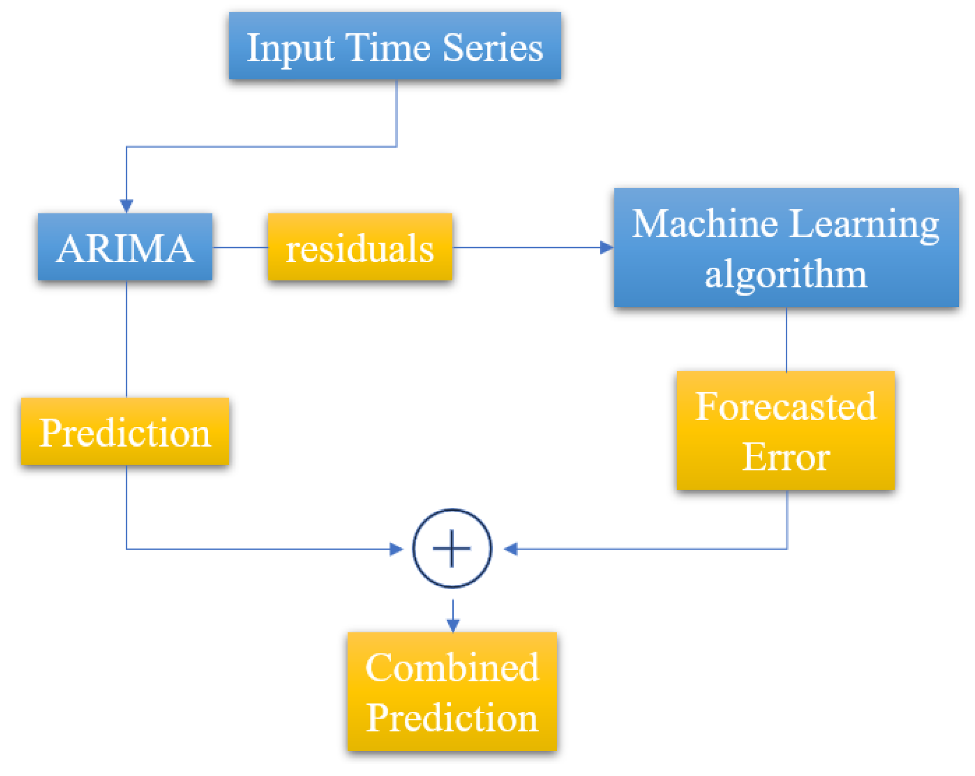
In the classic work by Zhang et al. [4], a hybrid model combining ARIMA and neural networks is proposed, aiming to exploit the capabilities of each model in terms of linear and non-linear modeling, respectively. The proposed methodology consists of two steps: In the first step, the ARIMA model is used to analyze the linear part of the problem, while in the second step, a neural network is developed to model the residuals of the ARIMA model. Since the classical ARIMA model cannot capture the non-linear structure of the data, the residuals of the linear model will contain information about the non-linearity. The outputs of the neural network can be used as predictors for the error terms of the ARIMA model. The results of this research showed that the hybrid model improves the prediction accuracy of both individual models. The proposed hybrid approach is presented graphically in Figure 6. A similar approach is used by Biswas et al. [57], Prajapati et al. [58], and Nie et al. [5] in different research fields and with a different selection of machine learning algorithms, combined with the ARIMA model.

4.1. Financial Data

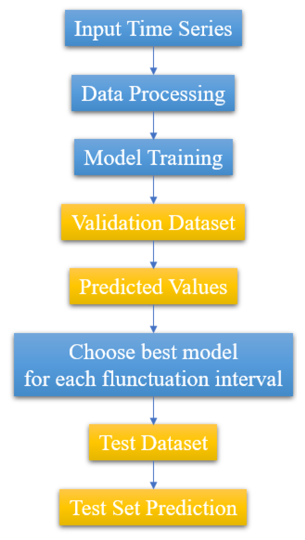
In the field of bitcoin price prediction research, which we have encountered in numerous works ([6,44,45]) the development of hybrid forecasting models is a widely used practice. The work of Nguyen et al. [44] which we already mentioned in the deep learning models paragraph, uses combinations of ARIMA with FFNN, CNN, LSTM, and SVR models to make bitcoin price time series predictions, as well as to compare these hybrid models. This particular work uses a different hybrid strategy than the one presented in Figure 6, namely, it utilizes each algorithm (ARIMA and ML-based) with respect to the fluctuation level observed for different time series intervals. The flowchart of this approach is depicted in Figure 7. The results of the work based on the RMSE and MAPE metrics, show that the performances of the four hybrid models are very close, with the best being given by the combination of ARIMA with the CNN model. Another example of a hybrid model application in the financial domain is the work by Zheng et al.

4.2. Weather

In terms of weather forecasting, research by Biswas et al. [57] suggests using a combination of regression and machine learning models to predict wind energy production over one, two, and seven day time horizons. The forecast is based on weather data such as wind speed and direction, air temperature and pressure, and density at the height of the measurement node. The preliminary results of this study indicate that the combination of ARIMA with Random Forest algorithms (ARIMA-RF) as well as the combination of ARIMA with Bayesian Regression and Classification Trees (BCART) help to improve the forecasting accuracy compared with the classical forecasting algorithm of ARIMA.

4.3. Healthcare Data

In the field of medical care and specifically regarding the prediction of COVID-19 cases, the work of Prajapati et al. [58] moves on three levels: Modeling the overall trend in the number of cases over time, short-term forecasting on the order of ten days in countries with extremely high population density such as India, and determining which algorithm presents the best metrics performance in accurately modeling the linear and non-linear characteristics of the case count time series. Various individual prediction models based on the Prophet, Holt-Winters, LSTM, and ARIMA algorithms were used, as well as the ARIMA-NARNN (Nonlinear Autoregressive Neural Network) hybrid model. The simple ARIMA algorithm performed better than other individual models; however, the hybrid combination of ARIMA and NARNN had the best overall performance, with RMSE values almost 35.3% better than ARIMA.

4.4. Utilities

In relation to the applications of SVMs in time series forecasting, the work of Nie et al. [5] deals with short-term load forecasting in energy transmission systems. Short-term load is a variable that is affected by many factors, and for this reason, it is difficult to make an accurate prediction with a single model. Utilizing the ARIMA algorithm to forecast the basic linear part of the load and the SVM algorithm to forecast the sensitive, non-linear part of the load, the paper presents a forecasting method based on a hybrid ARIMA and SVM model. ARIMA is used to forecast the daily load, and then the SVM model is used, aiming to correct the deviations from the previous forecasts. Due to their generalization ability and fast computation, SVMs show excellent performance in extracting the nonlinear part of the load and can be used to achieve the correction of the data deviation. The ARIMA-SVM hybrid model effectively combines the advantages of ARIMA and SVMs and through the simulation of a large sample of data, the results show that this hybrid model is much better than the two forecasting models applied separately.

4.5. Network Traffic

Finally, in the field of network parameter forecasting, we present the work of Ma et al. [59], where the ARIMA algorithm is combined with the Multi Layer Perceptron and the Multidimensional Support Vector Regression models in a hybrid approach to the network-wide traffic state forecasting problem. An increased predictive performance is observed in relation to the statistical forecasting method in cases where the network traffic is considered both at a local and global scale with the incorporation of the hybrid prediction model. An interesting change in the hybrid model workflow with respect to the previously mentioned studies is the fact that in this case the ARIMA algorithm is used after the neural network in order to post-process the ML model residuals. This is also, according to the authors, “necessary and a warrant at least for the situation where the time series data are not sufficiently long”.

The specific work aims to predict the traffic state for a small city area based on the measurement and prediction of three macroscopic traffic variables: traffic volume, speed, and occupancy. The dataset is comprised of time series collected from a network of detectors along the Highway Ayalon in Tel Aviv, Israel. The proposed approach can not only capture the network-wide co-movement pattern of traffic flows in the transportation system but also seize location-specific traffic characteristics as well as the sharp nonlinearity of macroscopic traffic variables. The case study indicates that the accuracy of prediction can be significantly improved when both network-scale traffic features and location-specific characteristics are taken into account.

5. Discussion and Practical Evaluation

In this paper, a series of works on different areas of time series analysis and forecasting were selectively presented, with the aim of comparing the classic ARIMA forecasting algorithms with machine learning and deep learning models. As we see in the consolidated representation of these tasks in Table 2, Table 3, Table 4 and Table 5 the used metrics, based on which the comparison of each algorithm with the ARIMA technique was performed, are similar for the majority of the tasks.

Table 5. Summary of studies comparing ARIMA and Hybrid Models in time series forecasting.

Article	Algorithms	Metrics	Dataset
Zhang et al. [4]	ARIMA/ANN	MSE	variety
		MAD
Nguyen et al. [44]	ARIMA/FFNN	RMSE	bitcoin price
	ARIMA/CNN	MAPE
	ARIMA/LSTM
	ARIMA/SVR
Biswas et al. [57]	ARIMA/RF	NMAE	wind power
	ARIMA/BCART
Prajapati et al. [58]	ARIMA/NARNN	RMSE	COVID-19 cases
Nie et al. [5]	ARIMA/SVM	MAPE	short-term load forecasting
		RMSE
Ma et al. [59]	NN/ARIMA	MSE	network-wide
	MSVR/ARIMA	MAPE	traffic

Table 5. Summary of studies comparing ARIMA and Hybrid Models in time series forecasting.

Article	Algorithms	Metrics	Dataset
Zhang et al. [4]	ARIMA/ANN	MSE	variety
		MAD
Nguyen et al. [44]	ARIMA/FFNN	RMSE	bitcoin price
	ARIMA/CNN	MAPE
	ARIMA/LSTM
	ARIMA/SVR
Biswas et al. [57]	ARIMA/RF	NMAE	wind power
	ARIMA/BCART
Prajapati et al. [58]	ARIMA/NARNN	RMSE	COVID-19 cases
Nie et al. [5]	ARIMA/SVM	MAPE	short-term load forecasting
		RMSE
Ma et al. [59]	NN/ARIMA	MSE	network-wide
	MSVR/ARIMA	MAPE	traffic

In the comparisons of the individual machine learning models with the ARIMA algorithm, a large part of the applications indicate the superiority of the former based on the metrics used. However, there were a subset of studies in which ARIMA demonstrated higher predictive accuracy. We will refer to these studies in the rest of the present chapter in order to practically evaluate the performance of the ARIMA against the machine learning models and to uncover the circumstances (either dataset or model-dependent) under which the statistical approach exhibits superior performance in the task of time-series forecasting.

• ARIMA over SVM Models

In the case of SVM algorithms, in the work of Zhang et al. [24] on drought prediction, the ARIMA algorithm had clearly better prediction performance based on various metrics, compared with the selected WNN and SVM models (Section 3.1.4). According to the authors of this paper, WNN and SVM machine learning models are not always superior to traditional ARIMA models in drought prediction. Different forecasting methods can be used for different geographic regions, and it would be subsequently advised for the data characteristics to be investigated in order to select the appropriate forecasting model.

This conclusion is consistent with the result of the work of Al Amin et al. [25], in which ARIMA performed better than SVM networks in load prediction when the load was linear (Section 3.1.5). As ARIMA is much more robust and efficient at analyzing linear time series, its choice over machine learning algorithms should primarily depend on the linearity of the data. In a different application field, the work by Priyadarshini et al. [38] indicated the superiority of ARIMA, and SARIMA forecasting over multiple deep learning and tree-based forecasting models regarding anomaly detection in an IoT setting. However, this particular publication is focused on the application at hand rather than on the model comparison.

• ARIMA over Deep Learning Models

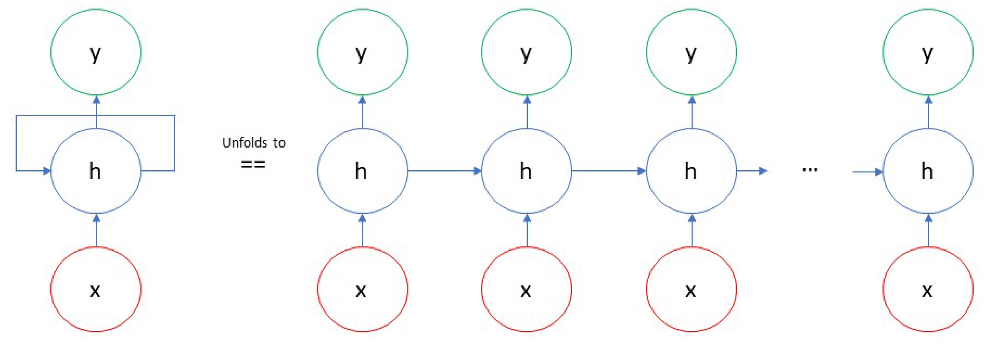
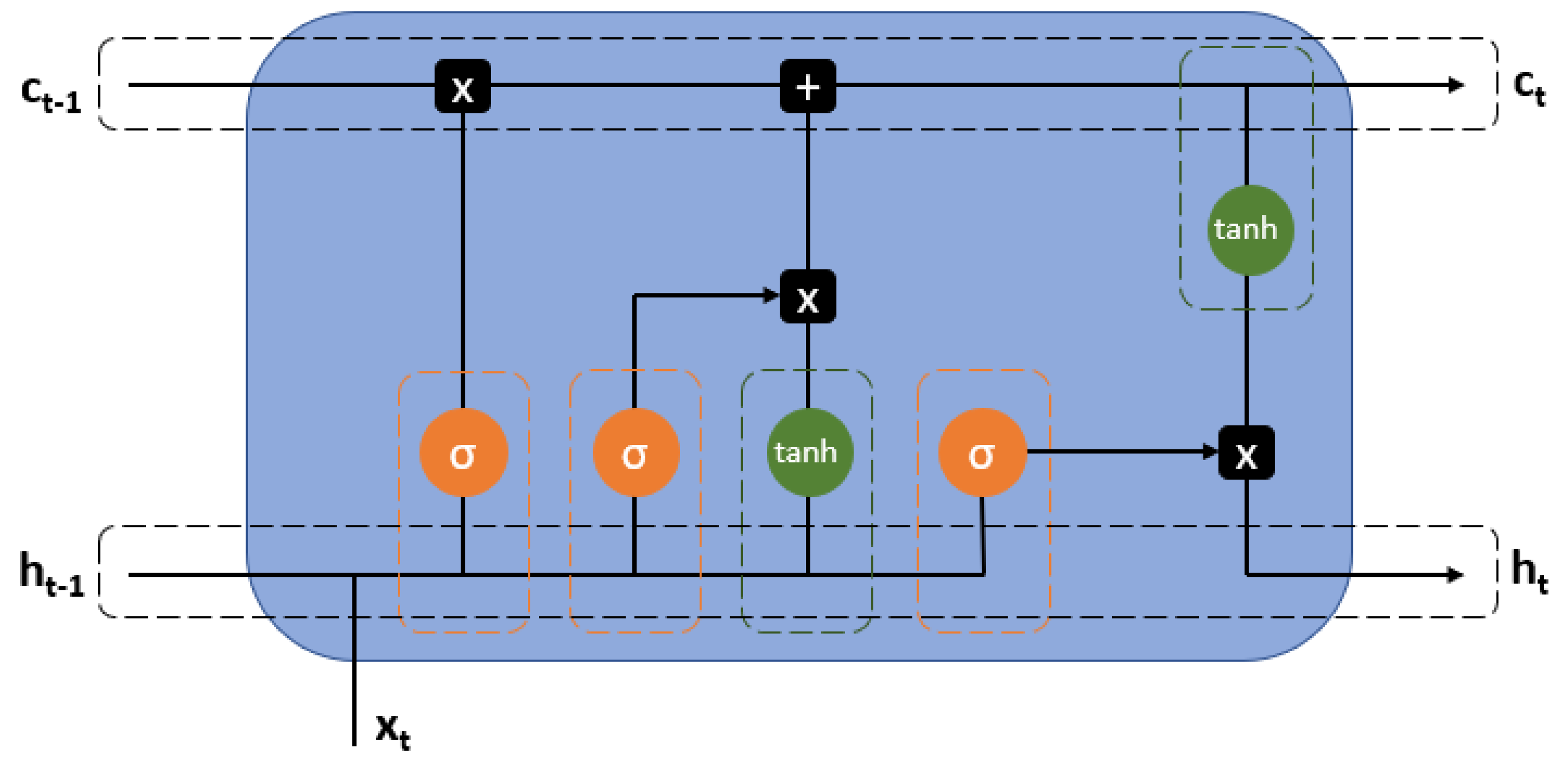
In the case of individual deep learning models vs. ARIMA, by introducing LSTM networks and the property of memory in the forecasting process, these models gain a great advantage over classical statistical forecasting methods, and this is shown by their dominance over ARIMA in the relevant literature. However, there are exceptions to this rule, which we will refer to below.

In the work of Paliari et al. [32] on stock index forecasting, the LSTM and XGBoost algorithms gave better forecasting results than ARIMA for all but two data sets, whose data values were significantly lower than the rest (Paragraph “Financial Data”). This fact probably indicates an advantage of statistical methods when the data is characterized by a limited range of values.

ARIMA methods prevail over deep learning algorithms in bitcoin price prediction applications in the works of Nguyen et al. [44] and Yamak et al. [6], and this result may be due to several factors, as the chosen values of the model parameters and the total amount of data can affect the results of the analysis. The volume of data in the work of Yamak et al. is relatively small, and RNN models usually perform well on more voluminous datasets, as previous studies have shown (Paragraph “Financial Data”). Regarding this particular observation, it is worth mentioning the related work of Cerqueira et al. [60], according to which machine learning methods improve their relative predictive performance over classical prediction algorithms as the data sample size grows.

In the work of Hua et al. [45], ARIMA is quite effective relative to LSTMs in making bitcoin price predictions in the short term, but as time goes on, it shows a decreasing rate of accuracy (Paragraph “Financial Data”).

In the work of ArunKumar et al. [51], the authors attempt to predict the rates of confirmed cases, recovered patients, and deaths from the COVID-19 disease in different countries of the world. For most cross-country time series data, the deep learning-based models (LSTM and GRU) outperform the statistical ARIMA and SARIMA models, with RMSE values 40 times smaller than those of the ARIMA models. However, in some countries, statistical models outperformed deep learning models (Paragraph “Healthcare Data”). Due to the highly dynamic nature of disease-specific data, the information they contain depends on the country of origin as well as the time at which they were generated. The shape of the data coming from some countries is non-linear, while ARIMA models are shown to perform better in modeling data that follows linear relationships. On the other hand, RNN models performed better in countries whose data were non-linear. These results once again confirm the conclusion made above, namely that since ARIMA is much more robust and efficient in linear time series analysis, its choice over machine learning algorithms should primarily depend on the linearity of the data. In this work, it is also interesting that while ARIMA is, according to the results, an ideal choice for modeling the rates of confirmed cases and recovered patients for some countries whose data have the appropriate profile, its performance is nevertheless very poor for modeling the number of deaths from COVID-19 in all countries, which is likely related to the increasing complexity of the data and the conditions that lead to the death of patients in general.

In the work of Liu et al. [54], which concerns the prediction of time series consisting of the measured wind speed in coastal areas, the SARIMA approach outperformed deep learning-based algorithms in prediction performance (Paragraph “Weather and Environmental Parameter Studies”). The authors of this paper argue that the SARIMA approach is more suitable for dealing with offshore wind speed forecasting because of its ability to directly support making predictions of seasonal elements on univariate datasets.

Finally, in the work of Spyrou et al. [17], ARIMA again outperforms LSTM models in predicting harbor area CO2 levels, which is likely related to the nature of the forecast data (Paragraph “Weather and Environmental Parameter Studies”).

• Hybrid Models over ARIMA

On the other hand, as far as the hybrid forecasting models are concerned, in any case and in the context of this work, they result in better forecasting performance compared with the single ARIMA model, as they combine modeling features both from the point of view of classical statistical algorithms and on the part of machine learning models, making them capable of dealing with predictive data at multiple levels of analysis.

• Final Remarks

There are various conclusions derived from the scientific literature cited in the previous paragraphs.

At first, we observe that the optimal choice of a forecasting algorithm can be different, for different versions of a dataset (e.g., different geographic regions in drought forecasting [24], different countries in modeling rates of confirmed and recovered cases of COVID-19 [50]) within the same forecasting task. The particular differences in the datasets’ nature, also inferred from the optimal model choice, can be of great value in a multitude of forecasting and modeling tasks and can be an important source of information for region characterization.

On the other hand, in some applications, it is the dataset characteristics inherent to the specific data driven network that drive the modeling choice. The seasonality of the data collected (e.g., wind speed forecasting [54]), the number of target variables, as well as a multitude of underlying causes and features (e.g., forecasting the number of COVID-19 deaths [50]) can shape the nature of a forecasting application. In our opinion, the systematic characterization of applications and datasets would be of great value to modeling applications in order to fully exploit the capabilities of big data and data-driven networks.

The ARIMA also exhibits better predictive performance than its machine learning counterparts, in cases where the available dataset is characterized by a limited range of values or a limited time-span ([6,32,45]). This observation can be attributed to the fact that machine learning, and especially deep learning models, require a large amount of data to train effectively. As a result, their performance can be inferior to statistical approaches for small datasets or for short-term forecasting.

The algorithmic nature of the ARIMA models provides some insight into their implementation value in the problem of time series forecasting. In comparison to complex machine learning models, ARIMA is a relatively explainable and intuitive approach that is widely used due to its flexibility and reliability. However, its focus on linear time dependencies in the data as well as its univariate modeling approach render it unsuitable for standalone application in forecasting complex real-world problems.

Apart from the details of the time series data, which can be a determining factor in the choice between ARIMA and machine learning models, an important aspect of the problem regards the computational and time complexity of the two approaches. In the case of machine learning forecasting models, a wider range of resources is needed, regarding the storage of the network architecture and weights, the training time, and the network optimization procedure, all of which are not necessary in the application of classical statistical algorithms. Furthermore, as the forecasting problem at hand becomes more complex and acquires longer time dependencies, so does its artificial intelligence modeling approach.

In

Table 6. Advantages and disadvantages of ARIMA over Artificial Intelligence models, regarding time series forecasting tasks.

Criterion	ARIMA	Artificial Intelligence
Model	Explainable	Regarded as a “black box”
	Flexible specification	Need training
	Reliable performance	Need optimization
	Designed to model dependencies	Better at modelling
	that can be linearizable	non-linear time dependencies
	through a single transformation
	Parameter specification	Standard training procedure
	depending on user-experience
Dataset	Suitable for small datasets	Need large datasets to train
	Missing values not important	Difficult modelling
		when values are missing
	Multiple seasonality	Complex modelling
	not handled natively
	Designed for univariate series	Handle multivariate datasets
	Sensitive to outliers	Depend on model complexity
	Assume data integrated	Data agnostic
	of a finite order
	Handles independent forecasting tasks	Joint forecast of multiple time series
Complexity	Low time complexity	Training and validation needed
	in general (depending on the model)
	Small computational requirements	Hardware and computational
	[61]	demands higher (depending on model)

, we present some aggregated results and observations based on the practical evaluation of the ARIMA versus the machine learning approach to the problem of time series forecasting.

6. Conclusions

While the classical statistical approach to the problem of time series forecasting is still practically relevant, recent advances in the machine learning field have introduced to the scientific community a variety of different models and a multitude of possible combinations of such models and their statistical counterparts. Nevertheless, the ARIMA method is prevailing in several cases, due to the nature of specific forecasting applications and datasets. Furthermore, even considering the sheer force of the machine learning models and their numerous predictive capabilities, they have significantly larger computational demands in contrast to the classic statistical models. The details of the forecasting problem at hand, the available resources, and the previous scientific approaches to a specific task should all be considered prior to proceeding with a single forecasting strategy.

References

1. Makridakis, S.; Spiliotis, E.; Assimakopoulos, V. Statistical and Machine Learning forecasting methods: Concerns and ways forward. PLoS ONE 2018, 13, e0194889. [Google Scholar] [CrossRef] [Green Version]
2. Dwivedi, Y.K.; Hughes, L.; Ismagilova, E.; Aarts, G.; Coombs, C.; Crick, T.; Duan, Y.; Dwivedi, R.; Edwards, J.; Eirug, A.; et al. Artificial Intelligence (AI): Multidisciplinary perspectives on emerging challenges, opportunities, and agenda for research, practice and policy. Int. J. Inf. Manag. 2021, 57, 101994. [Google Scholar]
3. Box, G.E.; Jenkins, G.M.; Reinsel, G.C.; Ljung, G.M. Time Series Analysis: Forecasting and Control; John Wiley & Sons: Hoboken, NJ, USA, 2015. [Google Scholar]
4. Zhang, G.P. Time series forecasting using a hybrid ARIMA and neural network model. Neurocomputing 2003, 50, 159–175. [Google Scholar] [CrossRef]
5. Nie, H.; Liu, G.; Liu, X.; Wang, Y. Hybrid of ARIMA and SVMs for short-term load forecasting. Energy Procedia 2012, 16, 1455–1460. [Google Scholar] [CrossRef] [Green Version]
6. Yamak, P.T.; Yujian, L.; Gadosey, P.K. A comparison between arima, lstm, and gru for time series forecasting. In Proceedings of the 2019 2nd International Conference on Algorithms, Computing and Artificial Intelligence, Sanya, China, 20–22 December 2019; pp. 49–55. [Google Scholar]
7. Time Series Data. Available online: https://www.clarify.io/learn/time-series-data (accessed on 12 July 2023).
8. Siami-Namini, S.; Tavakoli, N.; Namin, A.S. A comparative analysis of forecasting financial time series using arima, lstm, and bilstm. arXiv 2019, arXiv:1911.09512. [Google Scholar]
9. Wolpert, D.H.; Macready, W.G. No free lunch theorems for optimization. IEEE Trans. Evol. Comput. 1997, 1, 67–82. [Google Scholar] [CrossRef] [Green Version]
10. Bauer, A.; Züfle, M.; Herbst, N.; Kounev, S. Best practices for time series forecasting (tutorial). In Proceedings of the 2019 IEEE 4th International Workshops on Foundations and Applications of Self* Systems (FAS* W), Umea, Sweden, 16–20 June 2019; pp. 255–256. [Google Scholar]
11. Rundo, F.; Trenta, F.; di Stallo, A.L.; Battiato, S. Machine learning for quantitative finance applications: A survey. Appl. Sci. 2019, 9, 5574. [Google Scholar] [CrossRef] [Green Version]
12. Cheng, C.; Sa-Ngasoongsong, A.; Beyca, O.; Le, T.; Yang, H.; Kong, Z.; Bukkapatnam, S.T. Time series forecasting for nonlinear and non-stationary processes: A review and comparative study. IIE Trans. 2015, 47, 1053–1071. [Google Scholar] [CrossRef]
13. Siami-Namini, S.; Tavakoli, N.; Namin, A.S. A comparison of ARIMA and LSTM in forecasting time series. In Proceedings of the 2018 17th IEEE international conference on machine learning and applications (ICMLA), Orlando, FL, USA, 17–20 December 2018; pp. 1394–1401. [Google Scholar]
14. Xue, B.; Tong, N.; Xu, X.; He, X. Dynamical Short-Term Prediction of Rain Attenuation in W Band: A Time-Series Model with Simpler Structure and Higher Accuracy. IEEE Antennas Propag. Mag. 2019, 61, 77–86. [Google Scholar] [CrossRef]
15. RDocumentation: Auto.Arima: Fit Best ARIMA Model to Univariate Time Series. Available online: https://www.rdocumentation.org/packages/forecast/versions/8.21/topics/auto.arima (accessed on 12 July 2023).
16. Hyndman, R.J.; .Khandakar, Y. Automatic Time Series Forecasting: The forecast Package for R. J. Stat. Softw. 2008, 27, 1–22. [Google Scholar] [CrossRef] [Green Version]
17. Spyrou, E.D.; Tsoulos, I.; Stylios, C. Applying and comparing LSTM and ARIMA to predict CO levels for a time-series measurements in a port area. Signals 2022, 3, 235–248. [Google Scholar] [CrossRef]
18. Box, G.E.; Cox, D.R. An analysis of transformations. J. R. Stat. Soc. Ser. B Stat. Methodol. 1964, 26, 211–243. [Google Scholar] [CrossRef]
19. Cortes, C.; Vapnik, V. Support vector machine. Mach. Learn. 1995, 20, 273–297. [Google Scholar] [CrossRef]
20. Makala, D.; Li, Z. Prediction of gold price with ARIMA and SVM. J. Phys. Conf. Ser. 2021, 1767, 012022. [Google Scholar] [CrossRef]
21. Singh, S.; Parmar, K.S.; Makkhan, S.J.S.; Kaur, J.; Peshoria, S.; Kumar, J. Study of ARIMA and least square support vector machine (LS-SVM) models for the prediction of SARS-CoV-2 confirmed cases in the most affected countries. Chaos Solitons Fractals 2020, 139, 110086. [Google Scholar] [CrossRef] [PubMed]
22. Atique, S.; Noureen, S.; Roy, V.; Bayne, S.; Macfie, J. Time series forecasting of total daily solar energy generation: A comparative analysis between ARIMA and machine learning techniques. In Proceedings of the 2020 IEEE Green Technologies Conference (GreenTech), Oklahoma City, OK, USA, 1–3 April 2020; pp. 175–180. [Google Scholar]
23. Tiwari, S.; Kumaraswamidhas, L.; Garg, N. Comparison of svm and arima model in time-series forecasting of ambient noise levels. In Advances in Energy Technology: Select Proceedings of EMSME 2020; Springer: Singapore, 2022; pp. 777–786. [Google Scholar]
24. Zhang, Y.; Yang, H.; Cui, H.; Chen, Q. Comparison of the ability of ARIMA, WNN and SVM models for drought forecasting in the Sanjiang Plain, China. Nat. Resour. Res. 2020, 29, 1447–1464. [Google Scholar] [CrossRef]
25. Al Amin, M.A.; Hoque, M.A. Comparison of ARIMA and SVM for short-term load forecasting. In Proceedings of the 2019 9th Annual Information Technology, Electromechanical Engineering and Microelectronics Conference (IEMECON), Jaipur, India, 13–15 March 2019; pp. 1–6. [Google Scholar]
26. Liu, X.; Zhang, Y.; Zhang, Q. Comparison of EEMD-ARIMA, EEMD-BP and EEMD-SVM algorithms for predicting the hourly urban water consumption. J. Hydroinformatics 2022, 24, 535–558. [Google Scholar] [CrossRef]
27. Januschowski, T.; Wang, Y.; Torkkola, K.; Erkkilä, T.; Hasson, H.; Gasthaus, J. Forecasting with trees. Int. J. Forecast. 2022, 38, 1473–1481. [Google Scholar] [CrossRef]
28. Das, R.; Middya, A.I.; Roy, S. High granular and short term time series forecasting of PM2.5 air pollutant—A comparative review. Artif. Intell. Rev. 2022, 55, 1253–1287. [Google Scholar] [CrossRef]
29. Breiman, L.; Jerome Friedman, C.J.S.R.O. Classification and Regression Trees; Chapman and Hall/CRC: Boca Raton, FL, USA, 1984. [Google Scholar]
30. How Can Times Series Forecasting Be Done Using Random Forest? Available online: https://analyticsindiamag.com/how-can-times-series-forecasting-be-done-using-random-forest/#:~:text=A%20random%20forest%20regression%20model,forecasting%20for%20achieving%20better%20results.&text=Traditional%20time%20series%20forecasting%20models,to%20handle%20the%20continuous%20variables (accessed on 12 July 2023).
31. Sun, X.; Liu, M.; Sima, Z. A novel cryptocurrency price trend forecasting model based on LightGBM. Financ. Res. Lett. 2020, 32, 101084. [Google Scholar] [CrossRef]
32. Paliari, I.; Karanikola, A.; Kotsiantis, S. A comparison of the optimized LSTM, XGBOOST and ARIMA in Time Series forecasting. In Proceedings of the 2021 12th International Conference on Information, Intelligence, Systems & Applications (IISA), Chania Crete, Greece, 12–14 July 2021; pp. 1–7. [Google Scholar]
33. Alim, M.; Ye, G.H.; Guan, P.; Huang, D.S.; Zhou, B.S.; Wu, W. Comparison of ARIMA model and XGBoost model for prediction of human brucellosis in mainland China: A time-series study. BMJ Open 2020, 10, e039676. [Google Scholar] [CrossRef]
34. Lv, C.X.; An, S.-Y.; Qiao, B.-J.; Wu, W. Time series analysis of hemorrhagic fever with renal syndrome in mainland China by using an XGBoost forecasting model. BMC Infect. Dis. 2021, 21, 839. [Google Scholar] [CrossRef]
35. Fang, Z.; Yang, S.; Lv, C.; An, S.; Wu, W. Application of a data-driven XGBoost model for the prediction of COVID-19 in the USA: A time-series study. BMJ Open 2022, 12, e056685. [Google Scholar] [CrossRef] [PubMed]
36. Noorunnahar, M.; Chowdhury, A.H.; Mila, F.A. A tree based eXtreme Gradient Boosting (XGBoost) machine learning model to forecast the annual rice production in Bangladesh. PLoS ONE 2023, 18, e0283452. [Google Scholar] [CrossRef]
37. Zhang, L.; Bian, W.; Qu, W.; Tuo, L.; Wang, Y. Time series forecast of sales volume based on XGBoost. J. Phys. Conf. Ser. 2021, 1873, 012067. [Google Scholar] [CrossRef]
38. Priyadarshini, I.; Alkhayyat, A.; Gehlot, A.; Kumar, R. Time series analysis and anomaly detection for trustworthy smart homes. Comput. Electr. Eng. 2022, 102, 108193. [Google Scholar] [CrossRef]
39. Makridakis, S.; Spiliotis, E.; Assimakopoulos, V. The M5 competition: Background, organization, and implementation. Int. J. Forecast. 2022, 38, 1325–1336. [Google Scholar] [CrossRef]
40. Bojer, C.S.; Meldgaard, J.P. Kaggle forecasting competitions: An overlooked learning opportunity. Int. J. Forecast. 2021, 37, 587–603. [Google Scholar] [CrossRef]
41. Deep Learning. Available online: https://www.ibm.com/topics/deep-learning (accessed on 12 July 2023).
42. Hochreiter, S.; Schmidhuber, J. Long short-term memory. Neural Comput. 1997, 9, 1735–1780. [Google Scholar] [CrossRef]
43. Azari, A. Bitcoin price prediction: An ARIMA approach. arXiv 2019, arXiv:1904.05315. [Google Scholar]
44. Nguyen, D.T.; Le, H.V. Predicting the price of bitcoin using hybrid ARIMA and machine learning. In Proceedings of the Future Data and Security Engineering: 6th International Conference, FDSE 2019, Nha Trang City, Vietnam, 27–29 November 2019; Proceedings 6. Springer: Berlin/Heidelberg, Germany, 2019; pp. 696–704. [Google Scholar]
45. Hua, Y. Bitcoin price prediction using ARIMA and LSTM. E3S Web Conf. 2020, 218, 01050. [Google Scholar] [CrossRef]
46. Latif, N.; Selvam, J.D.; Kapse, M.; Sharma, V.; Mahajan, V. Comparative Performance of LSTM and ARIMA for the Short-Term Prediction of Bitcoin Prices. Australas. Account. Bus. Financ. J. 2023, 17, 256–276. [Google Scholar] [CrossRef]
47. Rhanoui, M.; Yousfi, S.; Mikram, M.; Merizak, H. Forecasting financial budget time series: ARIMA random walk vs LSTM neural network. IAES Int. J. Artif. Intell. 2019, 8, 317. [Google Scholar] [CrossRef]
48. Menculini, L.; Marini, A.; Proietti, M.; Garinei, A.; Bozza, A.; Moretti, C.; Marconi, M. Comparing prophet and deep learning to ARIMA in forecasting wholesale food prices. Forecasting 2021, 3, 644–662. [Google Scholar] [CrossRef]
49. Ning, Y.; Kazemi, H.; Tahmasebi, P. A comparative machine learning study for time series oil production forecasting: ARIMA, LSTM, and Prophet. Comput. Geosci. 2022, 164, 105126. [Google Scholar] [CrossRef]
50. Kırbaş, İ.; Sözen, A.; Tuncer, A.D.; Kazancıoğlu, F.Ş. Comparative analysis and forecasting of COVID-19 cases in various European countries with ARIMA, NARNN and LSTM approaches. Chaos Solitons Fractals 2020, 138, 110015. [Google Scholar] [CrossRef]
51. ArunKumar, K.; Kalaga, D.V.; Kumar, C.M.S.; Kawaji, M.; Brenza, T.M. Comparative analysis of Gated Recurrent Units (GRU), long Short-Term memory (LSTM) cells, autoregressive Integrated moving average (ARIMA), seasonal autoregressive Integrated moving average (SARIMA) for forecasting COVID-19 trends. Alex. Eng. J. 2022, 61, 7585–7603. [Google Scholar] [CrossRef]
52. De Saa, E.; Ranathunga, L. Comparison between ARIMA and Deep Learning Models for Temperature Forecasting. arXiv 2020, arXiv:2011.04452. [Google Scholar]
53. Verma, P.; Reddy, S.V.; Ragha, L.; Datta, D. Comparison of time-series forecasting models. In Proceedings of the 2021 International Conference on Intelligent Technologies (CONIT), Hubli, India, 25–27 June 2021; pp. 1–7. [Google Scholar]
54. Liu, X.; Lin, Z.; Feng, Z. Short-term offshore wind speed forecast by seasonal ARIMA-A comparison against GRU and LSTM. Energy 2021, 227, 120492. [Google Scholar] [CrossRef]
55. Zhou, K.; Wang, W.Y.; Hu, T.; Wu, C.H. Comparison of Time Series Forecasting Based on Statistical ARIMA Model and LSTM with Attention Mechanism. J. Phys. Conf. Ser. 2020, 1631, 012141. [Google Scholar] [CrossRef]
56. Azari, A.; Papapetrou, P.; Denic, S.; Peters, G. Cellular Traffic Prediction and Classification: A Comparative Evaluation of LSTM and ARIMA. In Discovery Science; Kralj Novak, P., Šmuc, T., Džeroski, S., Eds.; Springer International Publishing: Cham, Switzerland, 2019; pp. 129–144. [Google Scholar]
57. Biswas, A.K.; Ahmed, S.I.; Bankefa, T.; Ranganathan, P.; Salehfar, H. Performance analysis of short and mid-term wind power prediction using ARIMA and hybrid models. In Proceedings of the 2021 IEEE Power and Energy Conference at Illinois (PECI), Urbana, IL, USA, 1–2 April 2021; pp. 1–7. [Google Scholar]
58. Prajapati, S.; Swaraj, A.; Lalwani, R.; Narwal, A.; Verma, K. Comparison of traditional and hybrid time series models for forecasting COVID-19 cases. arXiv 2021, arXiv:2105.03266. [Google Scholar]
59. Ma, T.; Antoniou, C.; Toledo, T. Hybrid machine learning algorithm and statistical time series model for network-wide traffic forecast. Transp. Res. Part C Emerg. Technol. 2020, 111, 352–372. [Google Scholar] [CrossRef]
60. Cerqueira, V.; Torgo, L.; Soares, C. Machine learning vs statistical methods for time series forecasting: Size matters. arXiv 2019, arXiv:1909.13316. [Google Scholar]
61. Computational Complexity of Machine Learning Algorithms. Available online: https://medium.com/datadailyread/computational-complexity-of-machine-learning-algorithms-16e7ffcafa7d (accessed on 12 July 2023).
Figure 1. An example of a linearly separable problem of two classes in the two dimensional space. The support vectors are defined by the three samples on the lines that define the margin of optimal separation between the two classes.
Futureinternet 15 00255 g001
Figure 2. A graph of the support vector machine model architecture. The support vectors that define the regressive process are created by the feature space and the output space consists of the forecasted time series, which represent the objective variable.
Futureinternet 15 00255 g002
Figure 3. Basic architecture of an artificial neural network. By increasing the number of hidden layers (depth of the network), we also increase the capacity of the model.
Futureinternet 15 00255 g003
Figure 4. Building block of a recurrent neural network.
Futureinternet 15 00255 g004
Figure 5. Building block of a Long-short term memory network. The variables c and h represent the current state and the hidden state of the LSTM cell, while the input is represented by the x variable. The sigmoid gates inside the block constitute the forget, input and output gate respectively. The current state is updated with respect to the input, according to the sum of the current state and a combination of the input and the hidden state of the block.
Futureinternet 15 00255 g005
Figure 6. Flowchart of hybrid Arima and Machine Learning model for time series forecasting. This particular workflow is not the only one used in the scientific literature. Different combinations of the ARIMA and ML models have been proposed ([5,44]), based on the nature of the forecasting problem and the modeling approach.
Futureinternet 15 00255 g006
Figure 7. Flowchart of hybrid Arima and Machine Learning for time series forecasting, based on the fluctuation interval.
Futureinternet 15 00255 g007