1. Introduction
High platform station (HAPS) provides extremely broad coverage regions and a powerful line-of-sight (LoS) connectivity to terrestrial user equipment (UE) at the ground. As early as the 1990s, HAPS began to be paid attention to and studied through numerous research perspectives [
1].
Compared with Geostationary Earth Orbit (GEO) satellites that are orbiting at a height of about 36,000 km and Low Earth Orbit (LEO) satellites that are orbiting at a height of about 1200 km, HAPS operates at the stratosphere at heights between 20 and 50 km. Therefore, the Round Trip Time (RTT) of HAPS is much faster than that of GEO and LEO satellites. Furthermore, since HAPS is relatively close to the ground, the power density is approximately one million times that of a GEO satellite and approximately ten thousand times that of a LEO satellite, allowing HAPS to provide high-quality communication services to existing mobile devices [
2]. In addition, compared to other systems such as Starlink, which operates at an altitude of 340 km to 550 km [
3], HAPS is much less expensive in terms of both the launch and the communication costs. Nonetheless, it does not “pollute” the upper layers of the atmosphere with the space waste it creates.
It is recognized as one of the hot topics for Beyond 5G (B5G) and 6G mobile communications [
4,
5,
6,
7,
8]. With the necessary advanced materials and technological leaps, HAPS has been discussed as a viable technique.
With their potential and with the decrease in the cost of the technology behind it, they are expected to be massively deployed for consumer usage in the coming years as candidates for cellular coverage to provide service or to augment the capacity of other broadband service providers [
9].
S. Karapantazis et al. [
5] and A. K. Widiawan et al. [
10] summarized the essential technical aspects of HAPS systems and the current and potential applications of HAPS. In [
11], the authors studied the potential HAPS system architectures and deployment strategies in order to achieve global connectivity.
In [
12], White et al. studied the possibility of using HAPS to provide high data rate communications simultaneously to a number of trains in motion. According to the estimated and tracked Direction-of-Arrival (DoA) at the HAPS, they can control the parameters of the antenna array at the HAPS to transmit the beam to the UEs.
2. Related Work
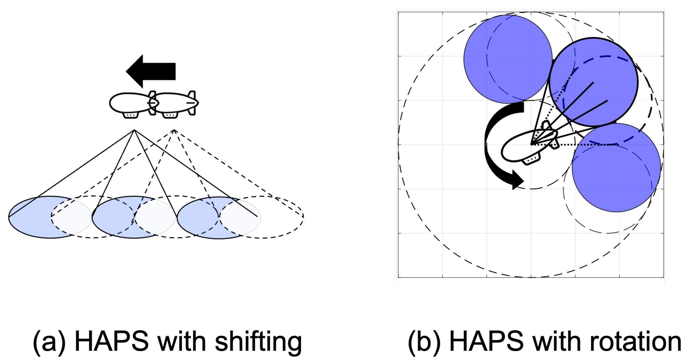
However, due to wind pressure, it is difficult for HAPS to remain stationary. Thus, the degradation of the users’ throughput and handovers to UEs’ end happened [
13,
14] after the HAPS coverage shifting. This kind of quasi-stationary state seriously impacts the performance of the communication system [
15]. Dessouky et al. [
16,
17] researched the problem of maximization of coverage through optimization of the parameters of the HAPS antenna arrays, and proposed an optimized way to minimize both the coverage gaps between cells and the excessive cell overlap. Yasser et al. [
18] studied the influence of handover performance when the HAPS is moved or rotated by winds. He et al. [
19] examined the swing state modeling of the cellular coverage geometry model and the influence of swing on handover. Many studies [
11,
20,
21,
22,
23,
24,
25,
26,
27,
28] on antenna control of HAPS proposed employing antenna control methods to prevent interference between surrounding cells and HAPSs to alleviate the decrease in received signal power caused by HAPS shifting or rotation. Kenji et al. [
20] proposed a beamforming method to reduce the impact of the degradation of system capacity caused by handover between two cells. Florin et al. [
21] analyzed the concentric circular antenna array (CCAA) and proposed a Genetic Algorithm (GA) to minimize the maximum side-lobe level (SLL). In [
22], Sun et al. further developed the discrete cuckoo search algorithm (IDCSA) used to reduce the maximum SLL under the constraint of a particular half-power bandwidth. To increase the system capacity, Dib et al. [
23] also researched SLL reduction. In contrast to existing approaches, they proposed a Symbiotic Organism Search (SOS) algorithm. The SOS algorithm requires no tuning of parameters, which makes it an attractive optimization method. In [
24], the particle swarm optimization (PSO) GA is used for reducing the SLL to improve the carrier-to-interference ratio (CIR). However, in high-dimensional space, PSO is easy to enter a local optimum, such as other GAs, and the iterative process’ convergence rate is low. These limitations motivate us to develop a new method with high convergence and better throughput performance.
With the rapid development of deep learning techniques, reinforcement learning (RL) is widely used in various fields including in 5G and B5G [
29,
30,
31]. F. B. Mismar et al. in [
32] used Deep
-Network (DQN) for online learning on how to maximize the users’ signal-to-interference plus noise ratio (SINR) and sum-rate capacity. The authors design a binary encoding for performing multiple relevant actions at once in the DQN structure. A. Rkhami et al. in [
33] used the RL method to solve the virtual network embedding problem (VNEP) in 5G and B5G. The authors considered that the conventional Deep Reinforcement Learning (DRL) usually obtains the sub-optimal solutions of VNEP, which leads to inefficient utilization of the resources and increases the cost of the allocation process. Thus, they proposed a relational graph convolutional neural network (GCNN) combined with DRL to automatically learn how to improve the quality of VNEP heuristics. In [
34], the authors proposed a deep learning integrated RL, which combined deep learning (DL) and RL. The DL is used for preparing the optimized beamforming codebook and the RL is used for selecting the best beam out of the optimized beamforming codebook based on the user movements.
According to those early works, we can find that the DRL technique can train the neural network with feedback from the environment. Thus, such as solving the beamforming problem in [
32] that using the DRL solution does not require the CSI to find the SINR-optimal beamforming vector. Moreover, different from model-free RL methods that need a huge optimal solution searching overhead for solving a complex problem, the DRL approach uses the DNN to predict the optimal solution without searching overhead. The DRL solution can be trained by the SINR feedback from users. Based on this motivation, we study the DRL and propose a novel DRL approach.
Contributions
The movement and rotation of the HAPS due to wind pressure can cause the cell range to shift, which in turn causes the degradation of users’ throughput and handovers between cells [
13,
14]. With the development of Global Positioning System (GPS) technology, HAPS can control itself to recover its original position state according to GPS positioning technology and thus restore the user signal quality. That being said, the position and rotation state of HAPS will always fluctuate within a certain range due to the unpredictable wind direction and wind force. However, we can improve throughput with beam steering. Thus, to solve the degradation of received power at UEs, we propose a Deep Reinforcement Learning Evolution (DRLEA) method. In our previous work [
35], we proposed a Fuzzy
-learning method. This method used Fuzzy logic in the model-free RL method named
-learning to control multiple searches in a single training step. Compared with the
-learning, the proposed Fuzzy
-learning method has a lower cost of action searching. However, we found that the throughput performance of the proposed Fuzzy
-learning method under non-uniform user distribution scenarios needs to be improved. Therefore, we proposed a DRLEA method for dynamic antenna control in the HAPS system to reduce the number of low-throughput users.
The proposed DRLEA considers that each iteration in the conventional DRL is a new generation. Starting from the first generation (the first iteration), DRLEA searches for the optimal solution in the current generation and trains the DNN to learn this evolutionary process. The DRLEA records the best result of the current generation as the historical optimal solution for guiding the next generation. If the current generation cannot find better solutions to reduce low throughput users, i.e. users whose throughput is lower than the median throughput prior to antenna parameters adjustment, the mutation happens (randomly selecting an action). The process is repeated until the specified execution time is reached. Compared with conventional RL methods, such as -learning-based and DQN-based methods, the proposed method can avoid the sub-optimal solution as much as possible. This is because, in every iteration a random initial set of parameters is used, and is then optimized, leading to less chances of falling into the local optimal.
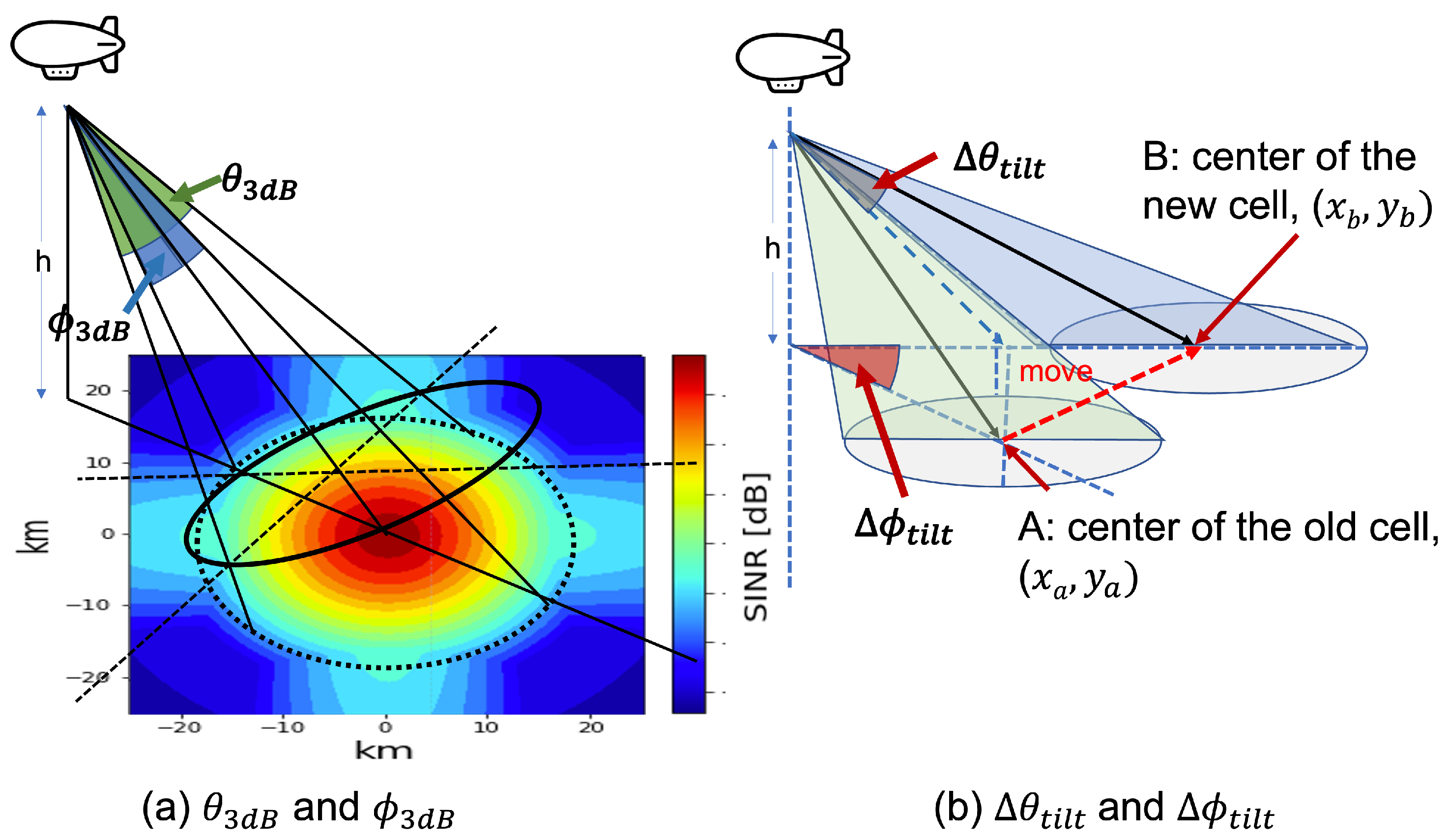
In addition, the performance of user throughput is closely related to the user’s SINR and bandwidth. We can improve the user’s SINR by gradually adjusting the antenna parameters based on the user’s feedback. As for the user’s dedicated bandwidth, it is only a function of the coverage of the antenna array in which the user is located as well as the number of users within that coverage area. Therefore, we do not necessarily need to know the channel state information (CSI) to design the beamforming matrix. Compared with obtaining an accurate CSI, obtaining the user location information, such as using the GPS technique, is less costly in terms of resources and time. It is nonetheless easier and computationally less expensive to adjust the antenna array parameters to account for the changes to the footprint of the users’ locations than that of their CSI.
Moreover, we implement three conventional methods, PSO, -learning, and DQN as benchmarks to evaluate the proposed DRLEA method and show that the proposed DRLEA is still reliable and efficient. This paper’s contributions can be outlined as follows:
We propose a novel DRLEA method that addresses the problem of dynamic control of the HAPS antenna parameters to decrease the number of users with low throughput. The proposed method combined the EA and DRL to avoid sub-optimal solutions.
We design a new loss function that includes not only -value of the predicted optimal action, but also the historical optimal solutions obtained from previous training.
Considering the random movement of HAPS caused by wind, we use the user’s throughput as a reward, which includes the users’ location information. Thus, with the same user distribution scenario and after training, the proposed method can quickly improve the users’ throughput under different types of HAPS movements. Even if the HAPS randomly moves again, the proposed approach can still reduce the number of low-throughput users.
The key notations used in this article are listed in
Table 1.
4. The Proposed DRLEA Approach
In this section, we present three algorithms that have been used as benchmarks and the proposed DRLEA algorithms for reducing the number of low-throughput users by dynamic antenna control. In the current paper, we address the case of a single HAPS movement. Our objective is to control only the HAPS in question (which has supposedly moved) to reduce the number of low-throughput users in the area it was serving before it moved. This means that no overlap or exchange of areas with surrounding HAPS will occur.
Therefore, we can simplify the system model as follows. We consider fixed-position HAPS around the HAPS in question that is moved due to wind pressure. Our target is to optimize the antenna parameters of this HAPS to reduce the number of users with low throughput. No handovers between the different HAPS is accounted for, and no new users are introduced to the coverage area of the HAPS in question.
4.1. Markov Decision Process
We define the state at time
t as
, and the selected action under the state
is
. Moreover, we consider using the four antenna parameters [
,
,
,
] at time
t as the state
. The action
is defined as the change of one set of antenna parameters, where
denotes the action set of the HAPS. To reduce the computational complexity, we use discrete antenna parameters to reduce the number of actions. Moreover, to perform the all actions at once, we design the action mapping list as shown in
Table 2. We assume that the number of antenna parameters of each antenna array is
, and the number of values of each antenna parameter is
. Thus, the number of actions of each antenna array is
, and the number of actions of a HAPS is
.
in
Table 2 indicates that antenna array 1 to antenna array
N performs action index 0.
The reward
with the state
and the action
A is represented by the Equation (
5).
where
K denotes the number of users,
denotes the sum of the throughput of the 50 percent users with the least throughput after performing the selected action
A, and
denotes the sum of the throughput of the 50 percent users with the least throughput under the initial state. Thus, the antenna parameters control problem can be represented by a Markov Decision Process (MDP):
, where
denotes an infinite state space,
p denotes the transition probability that characterizes the stochastic evolution of states in time, with the collection of probability distributions over the state space
, and
is the reward discount factor.
The goal is to find a deterministic optimal policy
, such that:
where
is the set of all admissible deterministic policies. At time step
t, HAPS selects an action simultaneously based on the policies
. The
function is shown as follows:
Thus, the optimal policy
can be obtained by:
where
denotes the next state,
denotes performing the action
that can obtain the maximum
value under the state
.
4.2. Conventional Methods
In this subsection, we will describe three methods that serve as benchmarks to solve the MDP.
4.2.1. -Learning
-learning is a kind of classical RL algorithm [
38]. To search the optimal
function,
-learning builds a
table to record the sum of existing
value
of the action
A for the current state
s. The
value is obtained by Equation (
9).
Here,
denotes the learning rate and
denotes performing the action
that can obtain the maximum
value under the state
. The details of the
-learning algorithm is shown in Algorithm 1.
| Algorithm 1 method for HAPS antenna control |
- Require:
, , , . - Ensure:
. - 1:
Build a table . - 2:
for epoch to E do - 3:
Initialize the antenna parameters. - 4:
for step to T do - 5:
Obtain the antenna parameters as state . - 6:
Randomly generates r in the range of (0,1). - 7:
if then - 8:
Randomly select an action - 9:
else - 10:
- 11:
end if - 12:
Perform the action A. - 13:
Get reward by Equation ( 5). - 14:
Update to . - 15:
Update the table : - 16:
- 17:
end for - 18:
end for
|
4.2.2. DQN
DQN is another classical RL [
39]. It calculates the
value of each action based on the reward returned from the environment states and uses the DNN instead of
table in
-learning method to predict the optimal
value. Therefore, we can obtain the
value with the state
s and the action
A based on Equation (
10).
Different from
-learning searching
table to obtain the optimal solution, the DQN method builds a deep neural network to learn the
value of each possible action corresponding to the input environment state. The details of the proposed DQN-based antenna control method are shown in Algorithm 2.
| Algorithm 2 DQN-based method for HAPS antenna control. |
- Require:
, , , . - Ensure:
- 1:
Initialize main network and target network . - 2:
Initialize experience reply memory . - 3:
for epoch to E do - 4:
Initialize the antenna parameters. - 5:
for step to T do - 6:
Obtain the antenna parameters as state . - 7:
Randomly generates r in the range of (0,1). - 8:
if then - 9:
Randomly select an action - 10:
else - 11:
- 12:
end if - 13:
Perform the action A. - 14:
Get reward by Equation ( 5). - 15:
Update to . - 16:
Store in the . - 17:
Get the output of the main network : . - 18:
Generate target value: - 19:
- 20:
. - 21:
Update the main network to minimize the loss function:
- 22:
end for - 23:
Update the target network: . - 24:
end for
|
In Algorithm 2,
E denotes the maximum number of epochs,
T denotes the maximum number of steps, and
denotes the weights of the deep neural network. We build two DQNs, one is the main network used for evaluating the
value of the action obtained by the
-greedy policy. This main network is trained during each step to estimate the approximate optimal action in the current state. The target network is updated with a copy of the latest learned parameters of the main network after each epoch. In other words, using a separate target network helps keep runaway bias from dominating the system numerically causing the estimated
values to diverge. Thus, using two DQNs instead of only one DQN can avoid the DQN algorithm to overestimate the true rewards [
40]. We calculate the reward
with the state
and the action
A by Equation (
5). In each step, we select an action based on the
-greedy method, and store the current state
, the selected action
A, the reward
, and the next state
into the experience replay memory
for training the main network
. Next, we train the main network
to minimize the loss function
, as shown in Equation (
11). After enough training, we input the current state
into the main network, then we can observed the predicted
value of all actions under the state
. Thus, the optimal action
can be obtained.
4.2.3. PSO
In this paper, we modify the PSO antenna control method in [
24] to reduce the number of low throughput users, as shown in Algorithm 3.
| Algorithm 3 PSO based algorithm for HAPS antenna control |
- 1:
Initialize the particles X and V. - 2:
for to E do - 3:
for to P do - 4:
- 5:
- 6:
Calculate by Equation ( 5) according to - 7:
if then then - 8:
- 9:
end if - 10:
if of other particles then - 11:
- 12:
end if - 13:
end for - 14:
end for - 15:
Output the best antenna parameters
|
Where denotes the antenna parameters of the k-th particle in the i-th iteration, denotes the k-th particle’s velocity (the change of antenna parameters) in the i-th iteration, denotes the best X of k-th particle until the i-th iteration, denotes the best X of all particles in all the iterations, and denote two independent learning rates, and are two independent random numbers for increasing randomness. The PSO algorithm randomly generates P particles to search the optimal antenna parameters X in each iteration and record it into . After each iteration, if the of the current iteration is larger than the previous , record it into as the optimal solution.
4.3. Deep Reinforcement Learning Evolution Algorithm
In the DQN method, the
value of each action is calculated based on the reward returned from the environment states. During the repeating of the experimental process, DQN can learn how to adjust antenna parameters to reduce the number of low-throughput users. Same with DQN approach, we obtain the
value by using the Equation (
10). However, using the DQN method for the HAPS system is difficult to search for the optimal solution. We use
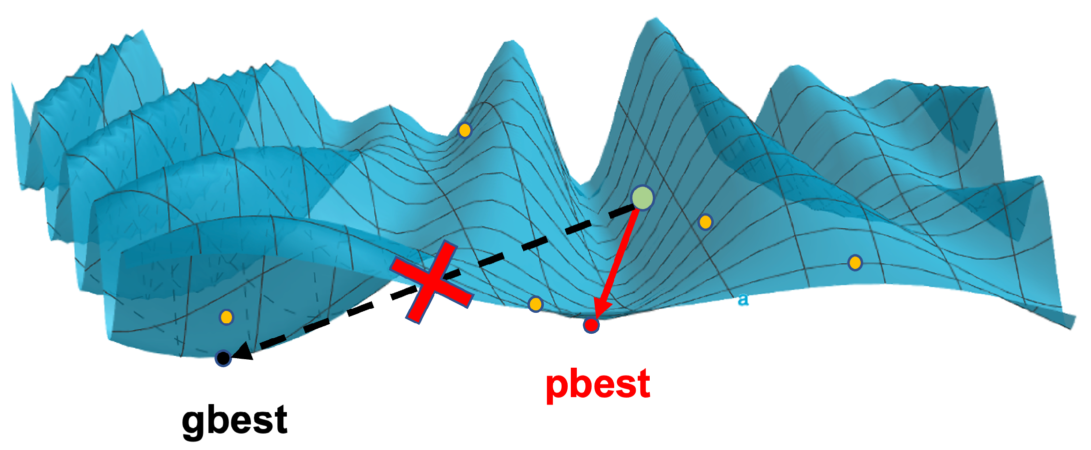
Figure 6 to explain the reason.
In
Figure 6, the ‘pbest’ is one of the sub-optimal solutions, the ‘gbest’ is the optimal solution. The DQN agent will adjust the antenna parameters step-by-step to find the optimal solution by using gradient descent. Nonetheless, if the initial state is located in the green point shown in
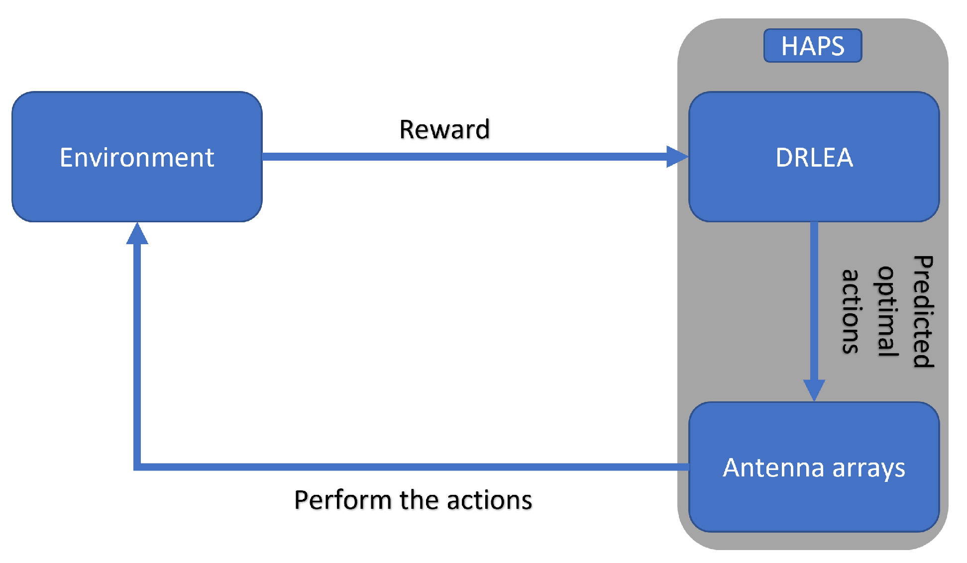
Figure 6, the DQN agent cannot obtain the optimal solution even using the Epsilon-greedy method for action selection. To address this problem, we design a novel DRLEA algorithm as shown in Algorithm 4. The workflow of the proposed method is shown in
Figure 7.
Different from the DQN method with the same initial state at the beginning of each training epoch, the DRLEA will randomly generate a different initial state for each training epoch, such as the yellow points shown in
Figure 6. For each epoch, the DRLEA performs many steps to search for the ’optimal’ solution (actually is a sub-optimal solution). After a training epoch, the DRLEA compares the ’optimal’ solution with the historical optimal solution and then keeps the better one. The details of the proposed DRLEA are shown in Algorithm 4.
Same with Algorithm 2, in Algorithm 4, we build two DNNs, the main network and the target network. We calculate the reward
with the state
and the action
A by Equation (
5). In step
t, we first select an action
A to maximize the
-value. If the reward
is lower than 0 or the reward of the previous step, the DRLEA will re-select and perform a random action from
. Next, we train the main network
to minimize the loss function
, as shown in Equation (
14). In Equation (
14), with the increase in the epochs, the influence of the current optimal solution is increased. After enough training, we input the current state
into the main network; then, we can obtain the predicted
value of all actions under the state
. Thus, the optimal action
can be obtained. After
E iterations, the optimal antenna parameters are recorded in
.
| Algorithm 4 Deep Reinforcement Learning Evolution Algorithm |
- Require:
, , , actions . - Ensure:
. - 1:
Initialize main network and target network . - 2:
Initialize experience reply memory . - 3:
Initialize with random matrices. - 4:
denotes the E different randomly generated antenna parameters. - 5:
. - 6:
Initialize and with zero matrices. - 7:
for to E do - 8:
Initialize the antenna parameters. - 9:
Initialize , . - 10:
for step to T do - 11:
- 12:
Perform the action A. - 13:
Get reward by Equation ( 5). - 14:
if then - 15:
Randomly select an action - 16:
Perform the action A. - 17:
end if - 18:
if then - 19:
Update : - 20:
end if - 21:
Update : . - 22:
Store in the . - 23:
Get the output of the main network : - 24:
. - 25:
Generate target value: - 26:
. - 27:
Update the main network to minimize the loss function:
- 28:
end for - 29:
if then - 30:
- 31:
- 32:
end if - 33:
Update the target network: . - 34:
end for
|
5. Simulation Results
5.1. Simulation Setting
To evaluate our proposed methods, we generate the four different non-uniform UEs distribution datasets obtained by [
41]. The four different user distributions are Tokyo, Osaka, Sendai, and Nagoya, as shown in
Figure 8.
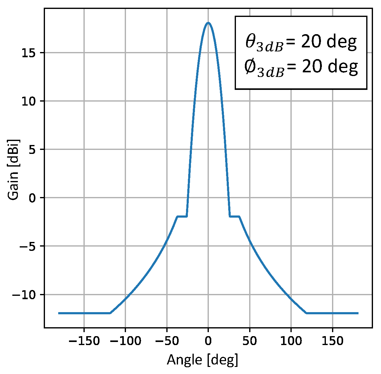
We assume that the HAPS works at a height of 20 km. Each HAPS can cover an area within a 20 km radius. The transmit power and bandwidth of each antenna array are 43 dBm and 20 Mhz, respectively. We consider that the transmission frequency is 2 GHz. Considering the interference between HAPSs, we set 18 HAPSs to surround 1 HAPS. We set the updated value of horizontal tilt, horizontal HPBW, vertical tilt, and vertical HPBW to 20 deg, 4 deg, 10 deg, and 4 deg, respectively. We use python to implement all simulation programs.
We set 100 epochs and 100 steps in each epoch, in the three RL-based approaches (-learning, DQN, and DRLEA). In the DQN and DRLEA, we set the learning rate of the neural network as 0.0001. The discount factor is 0.65 and the learning rate for value calculation is 0.75 in the three RL-based approaches. In the PSO approach, the number of iterations is 100, the number of particles is 100, and the and .
5.2. CDF of UE Throughput Performance
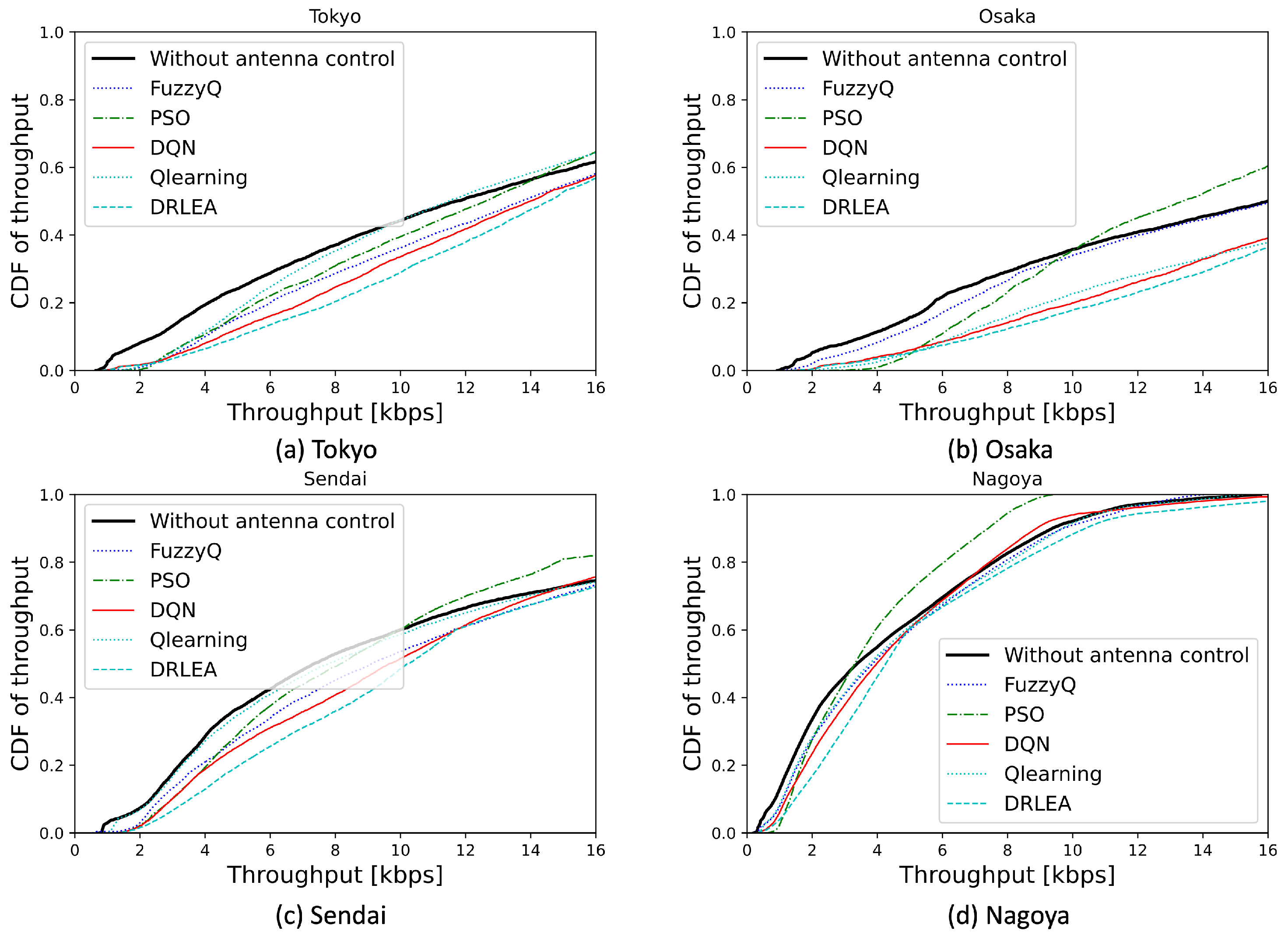
We train all the methods under the scenario where HAPS is rotated by 30 degrees, respectively, under four different user distributions.
Figure 9 shows the cumulative distribution function (CDF) of the users’ throughput under the rotation scenario.
In all the scenarios, the proposed DRLEA reduces the number of low-throughput users in the throughput range of kbps. In the case of Tokyo, the proposed algorithm achieves the best CDF performance in the throughput range of kbps. In the case of Osaka, the proposed method achieves the best performance in the throughput range of kbps. In the case of Sendai, the proposed method achieves the best performance in the throughput range of kbps. In the case of Nagoya, the proposed method achieves the best performance in the throughput range of kbps and kbps.
In the -learning, the Fuzzy -learning, and the DQN, which use the simple -greedy method for searching the optimal solution, are difficult to escape the local optimal. Even if we use the -greedy method to randomly select an action, the result is still close to the local optimal solution. However, in the proposed method, we consider using the strategy of EA. This strategy can make the result escape the local optimal by randomly setting the different initial states at the beginning of each epoch.
Similarly, the PSO method also uses the same strategy. In
Figure 9, we can find that in the
kbps throughput range, the PSO method has comparable or even better CDF of throughput performance than the other methods. In particular, in
Figure 9b, PSO achieves the best CDF performance in the
kbps throughput range. However, due to the high-dimensional space, the number of particles we set in our experiments is not enough for PSO to search for the optimal solution. It is still easy to fall into the local optimum.
Unlike PSO, which only targets the current global optimal solution and local optimal solution, the proposed method trains the neural network to adapt itself to avoid falling into the local optimal in a high-dimensional space.
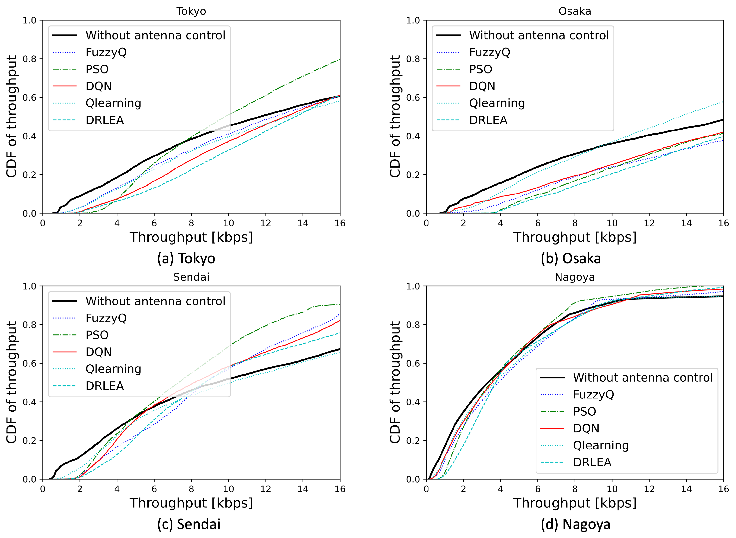
Moreover, we evaluate the proposed method under the shifting scenario. Here, we use the DRLEA and DQN methods, which are trained under the rotation case, and the other three methods are trained under the shifting scenario. As shown in
Figure 10, we can find that the DQN and the proposed DRLEA without retraining achieve comparable throughput performance to that of
-learning and Fuzzy
-learning with training in the HAPS left shift of the 5 km case. Since throughput is closely related to the user distribution, DNNs trained under the same user distribution know how to adjust the antenna parameters to reduce the number of low throughput users, even if HAPS moves again.
6. Conclusions
In this paper, we addressed the problem of the reduction of the number of users with low throughput caused by the movement of HAPS. To do so, a novel method named DRLEA was proposed. Different from the PSO and conventional RL methods, the proposed DRLEA method can adjust the antenna parameters without any searching overhead. We used the throughput of users for the reward calculation instead of using the received SINR. Using throughput for reward calculation will increase the computational overhead but it can make the DRLEA learn not only the SINR of users but also the location information of that. In other words, the proposed DRLEA method can improve the user’s SINR and bandwidth at the same time. Moreover, the proposed DRLEA combined EA with DRL to avoid sub-optimal solutions. A novel loss function was designed to train the DNN with the historical optimal solution to avoid the sub-optimal solutions.
Through simulations, we demonstrated that the proposed approach clearly improves the throughput of the users at the lower end of the spectrum. Compared with approaches such as the PSO and the -learning ones, the proposed DRLEA method achieves the best throughput performance under all the user distribution cases. Moreover, to prove the good robustness of the proposed DRLEA method, we use the proposed DRLEA, which is trained in the HAPS with a rotation scenario to control the antenna parameters under the shifting scenario. Through simulations, we demonstrated that, compared with the other three methods, which are trained under the HAPS with shifting, the proposed DRLEA method can achieve comparable throughput performances even without re-training.


 ,
, 


