Article

Online Optimization of Pickup and Delivery Problem Considering Feasibility

Graduate School of Information Science and Technoloty, Hokkaido University, Sapporo 060-0814, Japan
*
Author to whom correspondence should be addressed.
Future Internet 2024, 16(2), 64; https://doi.org/10.3390/fi16020064
Submission received: 27 December 2023 / Revised: 1 February 2024 / Accepted: 8 February 2024 / Published: 17 February 2024
(This article belongs to the Special Issue State-of-the-Art Future Internet Technology in Japan 2022-2023)

Abstract

:
A pickup and delivery problem by multiple agents has many applications, such as food delivery service and disaster rescue. In this problem, there are cases where fuels must be considered (e.g., the case of using drones as agents). In addition, there are cases where demand forecasting should be considered (e.g., the case where a large number of orders are carried by a small number of agents). In this paper, we consider an online pickup and delivery problem considering fuel and demand forecasting. First, the pickup and delivery problem with fuel constraints is formulated. The information on demand forecasting is included in the cost function. Based on the orders, the agents’ paths (e.g., the paths from stores to customers) are calculated. We suppose that the target area is given by an undirected graph. Using a given graph, several constraints such as the moves and fuels of the agents are introduced. This problem is reduced to a mixed integer linear programming (MILP) problem. Next, in online optimization, the MILP problem is solved depending on the acceptance of orders. Owing to new orders, the calculated future paths may be changed. Finally, by using a numerical example, we present the effectiveness of the proposed method.

1. Introduction

There has been much attention paid to control technologies for realizing a smart city [1]. In a smart city, many services using control technologies should be developed, such as transportation, energy distribution, healthcare, environmental monitoring, business, commerce, emergency response, and social activities. Moreover, in control technologies for a smart city, a cyber–physical system (CPS) plays an important role. A CPS is a system where physical and information components are deeply connected through a communication network. In a smart city, multiple physical components such as mobile robots are controlled by information systems, such as cloud servers. Hence, a plant in a smart city is modeled as a CPS. Thus, in a smart city and a CPS, it is important to develop a control method for multiple agents. In this paper, we focus on a control method for multiple agents.
Control of multiple agents has several applications and has been widely studied. In the control of multiple agents, there are several problem settings, such as the achievement of cooperative tasks and surveillance (patrol). A control specification in cooperative tasks may be given by linear temporal logic formulas [2,3,4,5,6,7,8,9,10,11,12,13,14,15,16]. Temporal logic is a logical system of rules and symbolism for representing, and reasoning about, propositions qualified in terms of time (for example, “I will eventually be hungry”). The surveillance problem is to find agents’ paths patrolling a given area as evenly as possible [8,17,18,19,20,21,22,23,24,25,26,27,28]. In problem settings on the control of multiple agents, model predictive control (MPC) is frequently used (see, e.g., [9,22,27]). MPC is a control method in which the control input is generated by solving at each time the finite-time optimal control problem (see, e.g., [29,30]). In other words, the control input is calculated based on the prediction using a mathematical model. MPC was frequently used in the control of chemical plants. In recent years, with the development of computers, MPC has been used in the control of several systems, such as automobiles. In the case where a target area is unknown and is changed in time, a model-free approach such as machine learning is effective (see, e.g., [31,32]). In this paper, we suppose that a target area is fixed and use a model-based approach.
In this paper, we focus on the pickup and delivery problem as one of the control problems of multiple agents. In recent years, the food delivery market has been expanding through the coronavirus epidemic. Efficient delivery from the restaurant to the customer is becoming more and more important. Such a problem of efficiently delivering goods received at a certain location to the desired location is called a pickup and delivery problem (see, e.g., [33,34,35,36,37,38,39,40,41]). Especially, the problem of updating routes by solving optimization problems at regular intervals is called an online pickup and delivery problem, which has been studied extensively in recent years (see, e.g., [42,43,44]).
In pickup and delivery problems, it is important to use electric vehicles and drones as agents. Electric vehicles and drones have the disadvantage of severe battery constraints. Hence, fuel constraints must be considered in pickup and delivery problems. In [45,46], a modeling method to handle the fueling of vehicles has been proposed. A fuel constraint in the proposed method is basically the same as in [45,46]. Refueling is different. In this paper, the fuel of a vehicle immediately becomes full by changing the battery. Furthermore, when electric vehicles and drones are used, demand forecasting is important (see, e.g., [47,48]). This is because more efficient moves are needed due to battery constraints. For example, many agents can be placed in advance at points where demand is concentrated. To the best of our knowledge, few results have been obtained.
In this paper, we propose an online pickup and delivery problem in which demand forecasting and fuel constraints are considered. First, we formulate the pickup and delivery problem. In this paper, the target area is given by an undirected graph. Constraints including fuel constraints are explained. Next, after the demand forecast is explained, the cost function is introduced. In a certain term in the cost function, we use the result of demand forecasting. Then, agents’ paths can be calculated according to the result of demand forecasting. That is, based on the policy of MPC, the real order and demand forecast are used. Even if the result of demand forecasting is different from real orders, the problem can be solved. This is because the result of demand forecasting is used in the cost function, not a constraint. Hence, we can guarantee the feasibility. Third, we explain the procedure of online optimization. Finally, we present a numerical example. Through a numerical example, we demonstrate that the feasibility is guaranteed by the proposed method.
The conference paper [49] is a preliminary version of this paper. In [49], the authors have considered both demand forecasting and fuel constraints. However, depending on the result of the demand forecasting, the optimization problem becomes infeasible. In this paper, this technical issue is overcome.
This paper is organized as follows. In Section 2, we formulate the pickup and delivery problem studied in this paper. After a mathematical model of the target area and the definition of the orders are explained, the constraints considered in this paper are explained. Demand forecasting in this paper is also explained. Finally, the cost function is explained. In Section 3, we explain the procedure of online optimization of the pickup and delivery problem. In Section 4, we present a numerical example to show the effectiveness of the proposed method. In Section 5, we conclude this paper.
The main contributions of this paper are highlighted as follows:
(i)
For pickup and delivery problems, fuel constraints are introduced to utilize electric vehicles and drones as agents.
(ii)
A pickup and delivery problem considering demand forecasting is newly formulated.
(iii)
The effectiveness of the proposed method is clarified through a numerical example.

2. Pickup and Delivery Problem
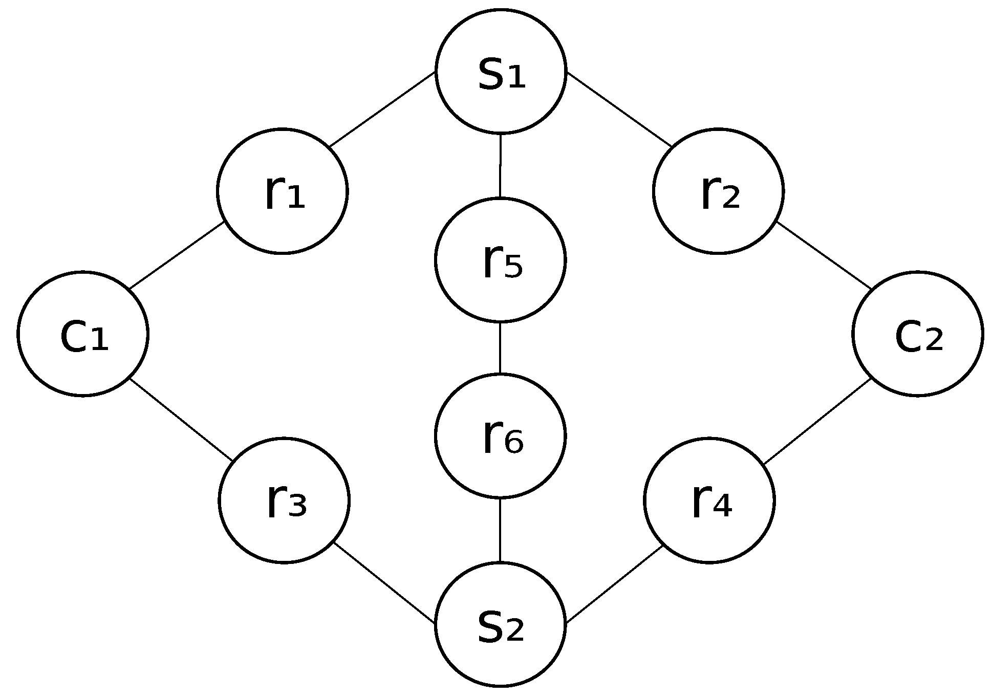
In this section, we formulate the pickup and delivery problem studied in this paper. First, we describe the preliminaries of the problem, which are the target area and the order notation. Next, we describe the constraints in the pickup and delivery problem. Finally, we describe the cost function in the pickup and delivery problem.

2.1. Preliminaries

We introduce some notations.
First, the target area in the pickup and delivery problem is given by the following undirected graph:
G = ( V , E ) ,
where there are the following:
  • V = S C R : the set of vertices ( S C R = );
  • S = { s 1 , s 2 , , s N } : the set of stores;
  • C = { c 1 , c 2 , , c M } : the set of customers;
  • R = { r 1 , r 2 , , r J } : the set of intermediate points between vertices;
  • E V × V : the set of edges.
Without the loss of generality, the set V can be represented by
V = { 1 , 2 , , N S , N + 1 , N + 2 , , N + M C , N + M + 1 , , N + M + J R } .
Let A = [ a i j ] { 0 , 1 } ( N + M + J ) × ( N + M + J ) denote the adjacency matrix of G , where if there is the edge between v i and v j , then a i j = 1 ; otherwise, a i j = 0 . An example of an undirected graph G = ( V , E ) is shown in Figure 1. We suppose that according to a given graph, an agent moves from some vertex to other one in unit time.
Next, notations about orders are introduced. We assume that new orders are received sequentially. Let τ i , i = 0 , 1 , 2 , denote the time that the delivery route may be changed. The initial update time τ 0 is set as τ 0 = 0 . We assume that at the update time τ i , there is at least one new order. Let O i denote the set of orders that are newly added at time t = τ i . The element o k of O i is given by the following form:
o k = ( s k , c k , T o k s , T o k c ) ,
where there are the following:
  • s k S : the store that received the order;
  • c k C : the customer who placed the order;
  • T o k s : the time that the goods are available for pickup;
  • T o k c : the time limit to complete the delivery.

2.2. Constraints

We formulate the following constraints in the pickup and delivery problem at the update time τ i .
  • Constraints on Agent Location: an agent can be located at only one vertex.
  • Constraints on Agent Movement: an agent can move according to a given graph.
  • Constraints on Orders: an order is assigned to an agent.
  • Constraints on the Set of Orders: an agent must receive the goods before delivery and must deliver those until a certain time.
  • Constraints on Agent Fuel: the fuel remaining for an agent must be equal to or greater than a certain value.
  • Constraints on Luggage: the number of goods that an agent can handle once is constrained.
We explain the details of these constraints.

2.2.1. Constraints on Agent Location

First, let N denote the finite set of agents. We introduce a binary variable vector p l ( t ) { 0 , 1 } | V | for the agent l N , where t { 0 , 1 , 2 , , } is discrete time. The j-th element p l , j ( t ) of p l ( t ) is 1 if the agent l is located at the vertex v j ; otherwise, it is 0. The constraint on the location of the agent l is given by
j = 1 | V | p l , j ( t ) = 1 , l N , t { τ i , , τ i + T f } ,
which implies that at time t, the agent l is located at only one vertex.

2.2.2. Constraints on Agent Movement

The movement of the agent l is constrained by the following inequality:
p l ( t ) A p l ( t + 1 ) , t { τ i , , τ i + T f 1 } ,
where the inequality sign (≤) holds element-wise. Equation (4) represents that the agent l moves only between vertices for which edges exist (see, e.g., [50,51,52]). We remark that (4) becomes the constraint on the agent movement when (3) is imposed.
For example, consider the undirected graph shown in Figure 1. Suppose that at time t, the agent l is located at the vertex s 1 . Then, the location candidates at time t + 1 are the vertices s 1 , r 1 , r 2 , and r 5 . Based on the notation of (1), the vertices s 1 , r 1 , r 2 , and r 5 correspond to 1, 5, 6, and 9, respectively. Because the first row of the adjacency matrix A is given by
1 0 0 0 1 1 0 0 1 0 ,
the above situation can be represented by the following inequality:
p l , 1 ( t ) p l , 1 ( t + 1 ) + p l , 5 ( t + 1 ) + p l , 6 ( t + 1 ) + p l , 9 ( t + 1 ) .
When at time t the agent l is located at the vertex s 1 , p l , 1 ( t ) = 1 holds. We remark that from (3), p l , j ( t ) = 0 , j 1 holds. Hence, under (3), either p l , 1 ( t + 1 ) , p l , 5 ( t + 1 ) , p l , 6 ( t + 1 ) , or p l , 9 ( t + 1 ) must be 1. This implies that the location candidates at time t + 1 are the vertices s 1 , r 1 , r 2 , and r 5 .

2.2.3. Constraints on Orders

For the agent l and the order o k , we introduce a binary variable y l , k as follows:
y l , k = 1 if   the   agent   l   is   responsible   for   the   order   o k , 0 otherwise .
As variables related to the agent l’s order receipt and delivery at time t, we also introduce binary variables z l , k pick ( t ) and z l , k deli ( t ) { 0 , 1 } as follows:
z l , k pick ( t ) = 1 if   the   agent   l   receives   the   goods   of   the   order   o k   at   time   t , 0 otherwise , z l , k deli ( t ) = 1 if   the   agent   l   delivers   the   goods   of   the   order   o k   at   time   t , 0 otherwise .
Assume that the vertex s k in the order o k corresponds to the vertex v i (i.e., the i-th element p l , i ( t ) of p l ( t ) ). Then, receiving the goods of the order o k at time t can be represented by the following expression:
[ z l , k pick ( t ) = 1 ] [ y l , k = 1 ] [ p l , i ( t ) = 1 ] , l , t .
Similarly, if c k corresponds to the i-th element p l , i ( t ) of p l ( t ) , then delivering the goods of order o k at time t can be represented by the following expression:
[ z l , k deli ( t ) = 1 ] [ y l , k = 1 ] [ p l , i ( t ) = 1 ] , l , t .
The relationship between y l , k , z l , k pick ( t ) , and z l , k deli ( t ) is represented by the following expressions:
[ y l , k = 1 ] t = T o k s τ i + T f z l , k pick ( t ) , k
[ y l , k = 1 ] t = T o k s τ i + T f z l , k deli ( t ) , k
We define two sets of orders P and D to represent the status of each order. The set P is the set of orders where the agent has not received the goods at the store. The set D is the set of orders where the agent has received the goods at the store and is in the process of delivery. Here, because there is only one agent responsible for each order, the following constraints must be imposed:
l y l , k = 1 , o k P D .

2.2.4. Constraints on the Set of Orders

The constraint on P is that the agent receives the goods before delivery and that the delivery time of the goods is equal to or earlier than the time limit τ i + T f . This constraint is represented by the following expressions:
l t = τ i t 1 z l , k pick ( t ) l t = τ i t 1 z l , k deli ( t ) 0 , t 1 { τ i , , τ i + T f } , o k P ,
l t = τ i τ i + T f z l , k deli ( t ) = 1 , o k P .
On the other hand, the constraint on D is that the time to deliver the goods must be equal to or earlier than the time limit τ i + T f . Hence, the constraint on D is expressed by the following expression:
l t = τ i τ i + T f z l , k deli ( t ) = 1 , o k D .

2.2.5. Constraints on Agent Fuel

When agents are implemented by using electric vehicles and drones, we need to consider fuel constraints.
We introduce the continuous variable q l ( t ) R as a variable representing the fuel of the agent l at time t. Let q 0 denote the agent’s maximum fuel. Suppose that the initial fuel is given by q l ( 0 ) = q 0 . The fuel q l ( t ) at time t is defined by
q l ( t ) = q 0 if   the   agent   l   is   located   at   the   vertex   in   S , q l ( t 1 ) 1 otherwise ,
which implies that the fuel is fully charged at the store vertex and decreases by one at the vertex, except for the store vertex.
The constraint on the fuel of the agent l is given by
q l ( t ) c , t { τ i , , τ i + T f 1 }
q l ( τ i + T f ) c f ,
where c , c f 0 are given constants. According to the policy of model predictive control, the terminal constraint may be different with other constraints. This difference can be realized via a method for choosing c and c f .

2.2.6. Constraints on Luggage

We introduce a variable X l ( t ) that represents the number of pieces of luggage carried by agent l at time t. Here, we assume that the weights of the packages are the same. Using z l , k pick ( t ) and z l , k deli ( t ) , the variable X l ( τ i ) can then be defined as
X l ( τ i ) = k ( z l , k pick ( 0 ) z l , k deli ( 0 ) ) if i = 0 , ( X l ( τ i ) ) i 1 otherwise   ( i 1 ) ,
where ( X l ( τ i ) ) i 1 is the value obtained via optimization at t = τ i 1 . In addition, X l ( t ) can be expressed as
X l ( t ) = X l ( t 1 ) + k ( z l , k pick ( t ) z l , k deli ( t ) ) ,
when t = τ i + 1 , , τ i + T f . Assume that the agent l can carry up to c w pieces of luggage, where c w is a given constant. The constraint on the number of pieces of luggage that the agent l carries at time t can be expressed as
X l ( t ) c w , l , t .
The variable X l ( t ) implies the number of pieces of luggage. In the case where the weights of the packages are different, the variable X l ( t ) is regarded as a total weight for the agent l via a simple modification.

2.3. Demand Forecast

In the conventional pickup and delivery problem, the paths of the agents are calculated at τ i , τ i + 1 , , max k T o k c ( max k T o k c represents the slowest time limit in the set of orders). In this paper, we consider using the demand forecast. It is expected that better paths are obtained by considering not only the time interval where there are orders but also the future where there are no orders.
In this paper, we assume that the number of agents (denoted by d j ( t ) ) required in the store s j at time t is given as the result of the demand forecast. In the next subsection, we explain how to use d j ( t ) .

2.4. Problem Formulation

Under the above preparations, we formulate the pickup and delivery problem at the update time τ i . The cost function to be minimized is defined as follows:
J i = c i , 1 + c i , 2 + c i , 3 .
We describe c i , 1 , c i , 2 , and c i , 3 in detail. At first, c i , 1 is defined as follows:
c i , 1 = w 1 t = τ i τ i + T f l N j C R p l , j ( t ) .
p l ( t ) { 0 , 1 } | V | is a binary variable vector for the agent l N , where t { 0 , 1 , 2 , , } is discrete time. The j-th element p l , j ( t ) of p l ( t ) is 1 if the agent l is located at the vertex v j ; otherwise, it is 0. The scalar w 1 is a constant representing the weights and is determined through trial and error. In other words, Equation (20) implies the sum of the time spent at the vertices, except for the store for all agents. By reducing the value of this term, the running cost of the agents can be reduced.
Next, c i , 2 is defined as follows:
c i , 2 = w 2 k α k ( T k T o k c ) ,
where T k is a variable that represents the time when the agent completes the delivery of order o k to the customer. Time T k can be expressed as
T k = l [ T o k c , . . . , τ i + T f ] z l , k deli ( T o k c ) z l , k deli ( τ i + T f ) ,
where z l , k deli ( t ) is a binary variable that is 1 if agent l delivers order o k at time t and 0 if it does not. In (22), the column vectors are all zero, except for one element. Therefore, from this expression, we can find T k when the value of z l , k deli ( t ) is equal to 1. The scalar α k is a variable that determines whether the delivery time of the order o k to be delivered meets the delivery deadline. The α k is defined as follows:
α k = 1 if T k T o k c , 0 otherwise .
where α k = 1 implies that the time T k when the order is delivered to the customer is later than the time limit T o k c to complete the delivery. The scalar w 2 is a constant representing the weights and is determined through trial and error.
In other words, Equation (21) is a summation of the delays in the delivery time. By reducing the value of this equation, we can obtain agent trajectories that satisfy the delivery time constraints of the order.
Finally, c i , 3 is defined as follows:
c i , 3 = w 3 t = τ i τ i + T f j | S | α j ( t ) ( σ j ( t ) d j ( t ) ) ,
where σ j ( t ) is a decision variable that represents the number of agents in store s j at time t. The constant d j ( t ) is given in advance (see Section 2.3). We assume that the demand forecast is a prediction of when, where, and how many orders will be placed. The α j ( t ) is a binary variable that determines whether the number of agents in store s j at time t satisfies the required number of agents in store s j obtained from the demand forecast. The α j ( t ) is defined as follows:
α j ( t ) = 1 if d j ( t ) σ j ( t ) , 0 otherwise ,
where α j ( t ) = 1 implies that the number of agents in store s j is less than the number of agents required for store s j obtained from the demand forecast. The scalar w 3 is a constant representing the weights and is determined through trial and error. In other words, Equation (24) is the sum of the number of agents that are less than the number of agents required for each store. By reducing the value of this equation, the agent trajectory can be obtained with more consideration given to demand forecasting.
The pickup and delivery problem at the update time τ i is given as follows.
Problem 1.
minimize ( 19 ) subject to ( 3 ) ( 18 ) , ( 22 ) , ( 23 ) , ( 25 ) .
Via a simple calculation (see, e.g., [52]), the constraint conditions (3)–(18), (22), (23), and (25) can be transformed into linear constraint conditions. In addition, the cost function is also transformed into a linear cost function. Hence, this problem is reduced to a mixed integer linear programming (MILP) problem.

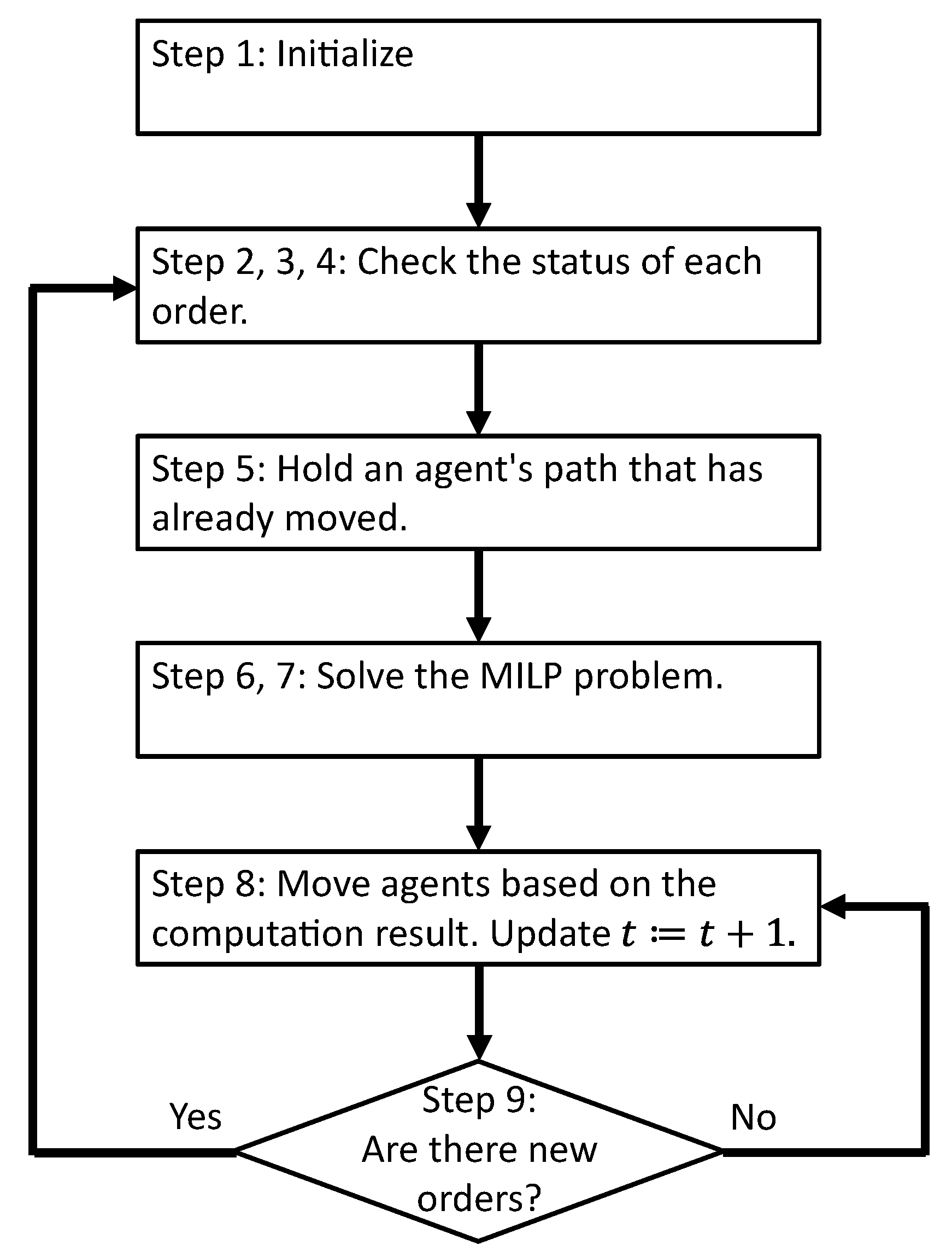
3. Online Optimization

For O i , P , and D , the online optimization of the pickup and delivery problem is performed as follows.
Procedure for online optimization of the pickup and delivery problem:
  • Step 1: If i = 0 , set P , D = , and t = 0 .
  • Step 2: For each o k P D , calculate the values of l t = τ i 1 τ i z l , k pick ( t ) and l t = τ i 1 τ i z l , k deli ( t ) .
  • Step 3: For o k P D , perform the following procedure.
    P : = P { o k } if l t = τ i 1 τ i z l , k pick ( t ) = 0 , P : = P { o k } , D = D { o k } if [ l t = τ i 1 τ i z l , k pick ( t ) = 1 ] [ l t = τ i 1 τ i z l , k deli ( t ) = 0 ] , P : = P { o k } , D = D { o k } if l t = τ i 1 τ i z l , k deli ( t ) = 1 .
  • Step 4: Update P : = P O i .
  • Step 5: For each order, if o k D , then update y l , k , l N to ( y l , k ) i 1 obtained via optimization at t = τ i 1 , that is,
    y l , k : = ( y l , k ) i 1 .
  • Step 6: For o k P , impose Equations (10) and (11) as a constraint. For o k D , impose (12) as a constraint.
  • Step 7: Solve the pickup and delivery problem at time t = τ i , adding the constraints in Equation (26).
  • Step 8: Based on the calculation results, move the agent. Update t : = t + 1 .
  • Step 9: If there are no orders at time t, return to Step 8. If there is an order, return to Step 2.
The outline of this procedure is shown in Figure 2.
In this procedure, the agents’ predicted paths may be changed by solving the optimization problem that is generated by receiving a new order. Because the agents’ predicted paths are changed online (real time), we call this procedure an online optimization.

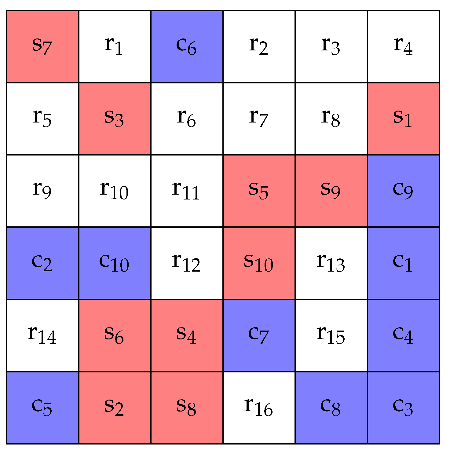
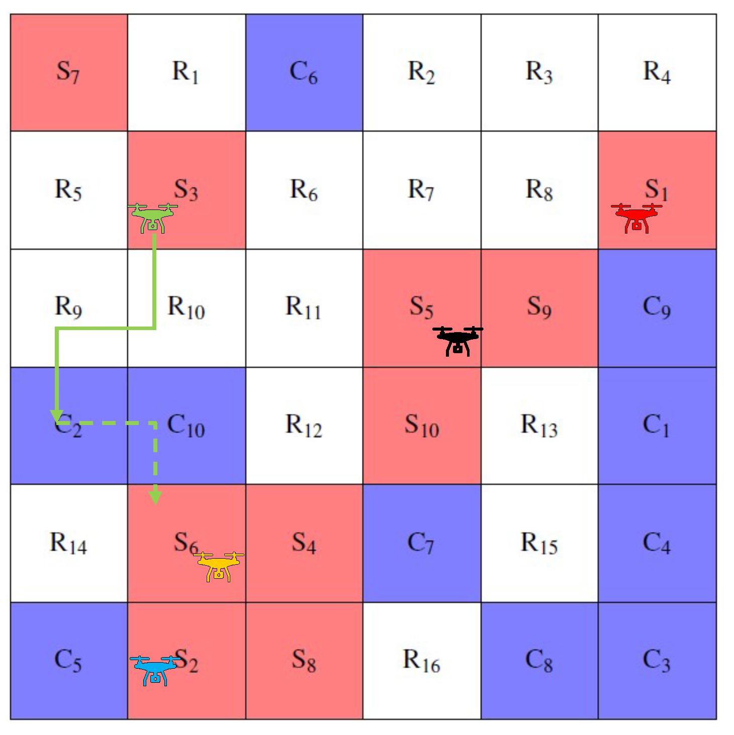
4. Numerical Example

In this section, we present a numerical example where the optimization problem is solvable even when the demand forecast deviates significantly from the actual order by considering the delivery constraints in the cost function. Here, we compare the proposed method with the existing method [49].

4.1. Preliminaries

Suppose that the target area is given by Figure 3. The number of vertices is set to | S | = 10 ,   | C | = 10 ,   and   | R | = 16 , and the graph is randomly arranged. The number of agents is set to 10, and the initial position is assumed to be one agent in each store. The maximum fuel of an agent is set to q 0 = 20 . All w 1 , w 2 , and w 3 in (20), (21), and (24) are set to 1. In addition, we set T f = 20 . We used a computer with an AMD Ryzen 5 5600X 6-Core Processor 3.70 GHz CPU and 32 GB of memory. The optimization problem at each update time was written using PuLP, which is a modeler written in Python. The solver used to compute the optimization problem was IBM ILOG CPLEX 20.1.0, which can be called from Python. The simulation result is outputted as the computation result of the Python program.
The order contents are given in Table 1. In the case of this order, the optimization problem is solved at times 0, 5, and 8. However, in the existing method, τ i + T f in the Equations (11) and (12) representing the delivery time constraints is T o k c . In other words, the existing method constrains the order delivery to be completed by the order delivery date, not within the time interval. In [49], the cost function J i is defined as follows, and the delivery time constraint is not considered in the cost function.
J i = t = τ i τ i + T f l j > | S | p l , j ( t )
The existing methods for demand forecasting consider the following inequalities.
l p l , j ( t ) d j ( t ) , ( j = 1 , 2 , , N )
The d j ( t ) used in Equations (24) and (28) are set to d 5 ( 8 ) = 4 and 0 in all other cases. This means that at time 8, store s 5 needs four agents, and there are no constraints for the other times or stores. However, the actual orders are not for store s 5 but for store s 4 , which means that the predictions of the stores that will receive the orders in the demand forecast are all wrong.

4.2. Calculation Results

Table 2 shows the results obtained for the case solved by the existing method. Table 3 shows the cost function values at each time for the existing method. Table 4 shows the results obtained for the case solved by the proposed method. Table 5 shows the value of the cost function at each time for the proposed method. Figure 4, Figure 5, Figure 6, Figure 7 and Figure 8 shows the obtained trajectories of the agents. The trajectories of the agents obtained at times 0 and 5 for the existing methods are shown in Figure 4 and Figure 6. The trajectories of the agents obtained at times 0, 5, and 7 for the proposed method are shown in Figure 5, Figure 7, and Figure 8. The solid line in Figure 4, Figure 5, Figure 6, Figure 7 and Figure 8 shows that the agent has luggage, while the dotted line shows that the agent does not have luggage. The thickness of the arrows in the figure indicates the number of pieces of luggage the agent is carrying.
From Table 2 and Table 4, only the proposed method can solve the problem at time 8 for the orders given in Figure 1. This is because in the case of the existing method, Equations (11) and (12) are not satisfied for orders o 2 and o 7 . On the other hand, in the case of the proposed method, we add to the cost function the amount of time past the delivery time constraint T o k c for the orders o 2 and o 7 from Table 4 and Table 5, respectively. Thus, the result at time 8 is solvable. Therefore, even when the demand forecast is significantly off and the delivery time constraints for all the orders are not met, an optimal solution that satisfies the conditions as much as possible can be obtained.

5. Conclusions

In this paper, we proposed an online pickup and delivery problem in which demand forecasting and fuel constraints were considered. First, we formulated the pickup and delivery problem with fuel constraints. Next, we introduced the cost function considering demand forecasting. After that, we explained the procedure of online optimization. Finally, through a numerical example, we presented the effectiveness of the proposed method.
In future work, we will consider practical applications. The problem formulation in this paper is relatively simpler than real food delivery services. It is important to extend the proposed method to the practical setting. We will consider many real scenarios and validate the proposed method. For large-scale scenarios, the computation time to solve an MILP problem becomes large (in this paper, as the first step, an MILP problem is solved by a conventional solver). It is also important to develop a distributed solution method, such that the problem is decomposed into small subproblems, and a parallel algorithm based on swarm optimization.

Author Contributions

Conceptualization, R.M., K.K. and Y.Y.; methodology, R.M. and K.K.; software, R.M.; writing, R.M. and K.K. All authors have read and agreed to the published version of the manuscript.

Funding

This work was partly supported by the JSPS KAKENHI Grant Numbers JP21H04558, JP22K04163, and JP23H01430.

Data Availability Statement

Data are contained within the article.

Conflicts of Interest

The authors declare no conflicts of interest.

References

  1. Cassandras, C.G. Smart cities as cyber-physical social systems. Engineering 2016, 2, 156–158. [Google Scholar] [CrossRef]
  2. Kloetzer, M.; Belta, C. Temporal logic planning and control of robotic swarms by hierarchical abstractions. IEEE Trans. Robot. 2007, 23, 320–330. [Google Scholar] [CrossRef]
  3. Kress-Gazit, H.; Fainekos, G.E.; Pappas, G.J. Temporal-logic-based reactive mission and motion planning. IEEE Trans. Robot. 2009, 25, 1370–1381. [Google Scholar] [CrossRef]
  4. Karaman, S.; Frazzoli, E. Linear temporal logic vehicle routing with applications to multi-UAV mission planning. Int. J. Robust Nonlinear Control 2011, 21, 1372–1395. [Google Scholar] [CrossRef]
  5. Ulusoy, A.; Smith, S.L.; Ding, X.C.; Belta, C. Robust multi-robot optimal path planning with temporal logic constraints. In Proceedings of the 2012 IEEE International Conference on Robotics and Automation, Saint Paul, MN, USA, 14–18 May 2012; pp. 4693–4698. [Google Scholar]
  6. Ding, X.; Lazar, M.; Belta, C. LTL receding horizon control for finite deterministic systems. Automatica 2014, 50, 399–408. [Google Scholar] [CrossRef]
  7. Raman, V.; Donzé, A.; Maasoumy, M.; Murray, R.M.; Sangiovanni-Vincentelli, A.; Seshia, S.A. Model predictive control with signal temporal logic specifications. In Proceedings of the 53rd IEEE Conference on Decision and Control, Los Angeles, CA, USA, 15–17 December 2014; pp. 81–87. [Google Scholar]
  8. Aksaray, D.; Leahy, K.; Belta, C. Distributed multi-agent persistent surveillance under temporal logic constraints. IFAC-PapersOnLine 2015, 48, 174–179. [Google Scholar] [CrossRef]
  9. Kobayashi, K.; Nagami, T.; Hiraishi, K. Optimal control of multi-vehicle systems with temporal logic constraints. IEICE Trans. Fundam. Electron. Commun. Comput. Sci. 2015, E98-A, 626–634. [Google Scholar] [CrossRef]
  10. Tumova, J.; Dimarogonas, D.V. Multi-agent planning under local LTL specifications and event-based synchronization. Automatica 2016, 70, 239–248. [Google Scholar] [CrossRef]
  11. Schillinger, P.; Bürger, M.; Dimarogonas, D.V. Simultaneous task allocation and planning for temporal logic goals in heterogeneous multi-robot systems. Int. J. Robot. Res. 2018, 37, 818–838. [Google Scholar] [CrossRef]
  12. Fujita, K.; Ushio, T. Optimal control of timed Petri nets under temporal logic constraints with generalized mutual exclusion. IEICE Trans. Fundam. Electron. Commun. Comput. Sci. 2022, 105, 808–815. [Google Scholar] [CrossRef]
  13. Fujita, K.; Ushio, T. Optimal Control of Colored Timed Petri Nets Under Generalized Mutual Exclusion Temporal Constraints. IEEE Access 2022, 10, 110849–110861. [Google Scholar] [CrossRef]
  14. Kinugawa, T.; Ushio, T. Finite-Horizon Optimal Spatio-Temporal Pattern Control under Spatio-Temporal Logic Specifications. IEICE Trans. Inf. Syst. 2022, 105, 1658–1664. [Google Scholar] [CrossRef]
  15. Oura, R.; Sakakibara, A.; Ushio, T. Reinforcement learning of control policy for linear temporal logic specifications using limit-deterministic generalized Büchi automata. IEEE Control Syst. Lett. 2020, 4, 761–766. [Google Scholar] [CrossRef]
  16. Terashima, K.; Kobayashi, K.; Yamashita, Y. Reinforcement Learning for Multi-Agent Systems with Temporal Logic Specifications. IEICE Trans. Fundam. Electron. Commun. Comput. Sci. 2024, E107-A, 31–37. [Google Scholar] [CrossRef]
  17. Beard, R.W.; McLain, T.W.; Nelson, D.B.; Kingston, D.; Johanson, D. Decentralized cooperative aerial surveillance using fixed-wing miniature UAVs. Proc. IEEE 2006, 94, 1306–1324. [Google Scholar] [CrossRef]
  18. Nigam, N.; Kroo, I. Persistent surveillance using multiple unmanned air vehicles. In Proceedings of the 2008 IEEE Aerospace Conference, Orlando, FL, USA, 27–29 October 2008; pp. 1–14. [Google Scholar]
  19. Elmaliach, Y.; Agmon, N.; Kaminka, G.A. Multi-robot area patrol under frequency constraints. Ann. Math. Artif. Intell. 2009, 57, 293–320. [Google Scholar] [CrossRef]
  20. Fu, J.G.M.; Ang, M.H. Probabilistic ants (PAnts) in multi-agent patrolling. In Proceedings of the 2009 IEEE/ASME International Conference on Advanced Intelligent Mechatronics, Singapore, 14–17 July 2009; pp. 1371–1376. [Google Scholar]
  21. Di Paola, D.; Naso, D.; Turchiano, B.; Cicirelli, G.; Distante, A. Matrix-based discrete event control for surveillance mobile robotics. J. Intell. Robot. Syst. 2009, 56, 513–541. [Google Scholar] [CrossRef]
  22. Ding, X.C.; Belta, C.; Cassandras, C.G. Receding horizon surveillance with temporal logic specifications. In Proceedings of the 49th IEEE Conference on Decision and Control (CDC), Atlanta, GA, USA, 15–17 December 2010; pp. 256–261. [Google Scholar]
  23. Nigam, N.; Bieniawski, S.; Kroo, I.; Vian, J. Control of multiple UAVs for persistent surveillance: Algorithm and flight test results. IEEE Trans. Control Syst. Technol. 2011, 20, 1236–1251. [Google Scholar] [CrossRef]
  24. Pasqualetti, F.; Franchi, A.; Bullo, F. On cooperative patrolling: Optimal trajectories, complexity analysis, and approximation algorithms. IEEE Trans. Robot. 2012, 28, 592–606. [Google Scholar] [CrossRef]
  25. Lin, X.; Cassandras, C.G. An optimal control approach to the multi-agent persistent monitoring problem in two-dimensional spaces. IEEE Trans. Autom. Control 2014, 60, 1659–1664. [Google Scholar] [CrossRef]
  26. Kajita, K.; Konaka, E. Hard-to-predict routing algorithm from intruders for autonomous surveillance robots. In Proceedings of the IECON 2018-44th Annual Conference of the IEEE Industrial Electronics Society, Washington, DC, USA, 21–23 October 2018; pp. 2540–2545. [Google Scholar]
  27. Masuda, R.; Kobayashi, K.; Yamashita, Y. Dynamic Surveillance by Multiple Agents with Fuel Constraints. IEICE Trans. Fundam. Electron. Commun. Comput. Sci. 2020, E103-A, 462–468. [Google Scholar] [CrossRef]
  28. Zuo, Y.; Tharmarasa, R.; Jassemi-Zargani, R.; Kashyap, N.; Thiyagalingam, J.; Kirubarajan, T.T. MILP formulation for aircraft path planning in persistent surveillance. IEEE Trans. Aerosp. Electron. Syst. 2020, 56, 3796–3811. [Google Scholar] [CrossRef]
  29. Mayne, D.Q.; Rawlings, J.B.; Rao, C.V.; Scokaert, P.O. Constrained model predictive control: Stability and optimality. Automatica 2000, 36, 789–814. [Google Scholar] [CrossRef]
  30. Mayne, D.Q. Model predictive control: Recent developments and future promise. Automatica 2014, 50, 2967–2986. [Google Scholar] [CrossRef]
  31. Xie, R.; Meng, Z.; Wang, L.; Li, H.; Wang, K.; Wu, Z. Unmanned aerial vehicle path planning algorithm based on deep reinforcement learning in large-scale and dynamic environments. IEEE Access 2021, 9, 24884–24900. [Google Scholar] [CrossRef]
  32. Liu, Y.; Vogiatzis, C.; Yoshida, R.; Morman, E. Solving reward-collecting problems with UAVs: A comparison of online optimization and Q-learning. J. Intell. Robot. Syst. 2022, 104, 35. [Google Scholar] [CrossRef]
  33. Dumas, Y.; Desrosiers, J.; Soumis, F. The pickup and delivery problem with time windows. Eur. J. Oper. Res. 1991, 54, 7–22. [Google Scholar] [CrossRef]
  34. Baker, B.M.; Ayechew, M. A genetic algorithm for the vehicle routing problem. Comput. Oper. Res. 2003, 30, 787–800. [Google Scholar] [CrossRef]
  35. Parragh, S.N.; Doerner, K.F.; Hartl, R.F. A survey on pickup and delivery problems: Part I: Transportation between customers and depot. J. Betriebswirtschaft 2008, 58, 21–51. [Google Scholar] [CrossRef]
  36. Salzman, O.; Stern, R. Research challenges and opportunities in multi-agent path finding and multi-agent pickup and delivery problems. In Proceedings of the 19th International Conference on Autonomous Agents and MultiAgent Systems, Auckland, New Zealand, 9–13 May 2020; pp. 1711–1715. [Google Scholar]
  37. Sun, P.; Veelenturf, L.P.; Hewitt, M.; Van Woensel, T. Adaptive large neighborhood search for the time-dependent profitable pickup and delivery problem with time windows. Transp. Res. Part E Logist. Transp. Rev. 2020, 138, 101942. [Google Scholar] [CrossRef]
  38. Koç, Ç.; Laporte, G.; Tükenmez, İ. A review of vehicle routing with simultaneous pickup and delivery. Comput. Oper. Res. 2020, 122, 104987. [Google Scholar] [CrossRef]
  39. Wang, J.; Sun, Y.; Zhang, Z.; Gao, S. Solving multitrip pickup and delivery problem with time windows and manpower planning using multiobjective algorithms. IEEE/CAA J. Autom. Sin. 2020, 7, 1134–1153. [Google Scholar] [CrossRef]
  40. Jun, S.; Lee, S.; Yih, Y. Pickup and delivery problem with recharging for material handling systems utilising autonomous mobile robots. Eur. J. Oper. Res. 2021, 289, 1153–1168. [Google Scholar] [CrossRef]
  41. Ma, Y.; Hao, X.; Hao, J.; Lu, J.; Liu, X.; Xialiang, T.; Yuan, M.; Li, Z.; Tang, J.; Meng, Z. A hierarchical reinforcement learning based optimization framework for large-scale dynamic pickup and delivery problems. Adv. Neural Inf. Process. Syst. 2021, 34, 23609–23620. [Google Scholar]
  42. Berbeglia, G.; Cordeau, J.F.; Laporte, G. Dynamic pickup and delivery problems. Eur. J. Oper. Res. 2010, 202, 8–15. [Google Scholar] [CrossRef]
  43. Bartlett, K.; Lee, J.; Ahmed, S.; Nemhauser, G.; Sokol, J.; Na, B. Congestion-aware dynamic routing in automated material handling systems. Comput. Ind. Eng. 2014, 70, 176–182. [Google Scholar] [CrossRef]
  44. Fransen, K.; Van Eekelen, J.; Pogromsky, A.; Boon, M.A.; Adan, I.J. A dynamic path planning approach for dense, large, grid-based automated guided vehicle systems. Comput. Oper. Res. 2020, 123, 105046. [Google Scholar] [CrossRef]
  45. Purba, D.S.D.; Kontou, E.; Vogiatzis, C. Evacuation route planning for alternative fuel vehicles. Transp. Res. Part Emerg. Technol. 2022, 143, 103837. [Google Scholar] [CrossRef]
  46. Purba, D.S.D.; Balisi, S.; Kontou, E. Refueling Station Location Model to Support Evacuation of Alternative Fuel Vehicles. Transp. Res. Rec. 2024, 2678, 521–538. [Google Scholar] [CrossRef]
  47. Regue, R.; Recker, W. Proactive vehicle routing with inferred demand to solve the bikesharing rebalancing problem. Transp. Res. Part E Logist. Transp. Rev. 2014, 72, 192–209. [Google Scholar] [CrossRef]
  48. Hess, A.; Spinler, S.; Winkenbach, M. Real-time demand forecasting for an urban delivery platform. Transp. Res. Part Logist. Transp. Rev. 2021, 145, 102147. [Google Scholar] [CrossRef]
  49. Matsuoka, R.; Kobayashi, K.; Yamashita, Y. Online Optimization of Pickup and Delivery Problem Considering Demand Forecasting. In Proceedings of the 2023 IEEE 12th Global Conference on Consumer Electronics, Nara, Japan, 10–13 October 2023; pp. 879–880. [Google Scholar]
  50. Bemporad, A.; Morari, M. Control of systems integrating logic, dynamics, and constraints. Automatica 1999, 35, 407–427. [Google Scholar] [CrossRef]
  51. Kobayashi, K.; Imura, J.i. Deterministic finite automata representation for model predictive control of hybrid systems. J. Process Control 2012, 22, 1670–1680. [Google Scholar] [CrossRef]
  52. Williams, H.P. Model Building in Mathematical Programming; John Wiley & Sons: Hoboken, NJ, USA, 2013. [Google Scholar]
Figure 1. Example of an undirected graph G = ( V , E ) , where | S | = N = 2 , | C | = M = 2 , and | R | = J = 6 .
Futureinternet 16 00064 g001
Figure 2. Outline of the procedure of online optimization.
Futureinternet 16 00064 g002
Figure 3. Target area, where an agent can move to an up/down/left/right vertex.
Futureinternet 16 00064 g003
Figure 4. Results at time 0 with existing method.
Futureinternet 16 00064 g004
Figure 5. Results at time 0 with proposed method.
Futureinternet 16 00064 g005
Figure 6. Results at time 5 with existing method.
Futureinternet 16 00064 g006
Figure 7. Results at time 5 with proposed method.
Futureinternet 16 00064 g007
Figure 8. Results at time 8 with proposed method.
Futureinternet 16 00064 g008
Table 1. Order details.
Order s k c k T o k s T o k c
o 1 s 3 c 2 07
o 2 s 2 c 3 512
o 3 s 1 c 4 512
o 4 s 4 c 5 813
o 5 s 4 c 6 813
o 6 s 4 c 8 813
o 7 s 4 c 9 813
Table 2. Results with the existing method.
Results at Time 0Results at Time 5Results at Time 8
Order Agent Pickup Time Delivery Time Agent Pickup Time Delivery Time Agent Pickup Time Delivery Time
o 1 305305
o 2 259
o 3 1510
o 4
o 5
o 6
o 7
Table 3. Values of the cost function at each time in the existing method.
TimeCost Function J i
05
512
8Infeasible
Table 4. Results with the proposed method.
Results at Time 0Results at Time 5Results at Time 8
OrderAgentPickup TimeDelivery TimeAgentPickup TimeDelivery TimeAgentPickup TimeDelivery Time
o 1 303303303
o 2 25122514
o 3 159159
o 4 31013
o 5 8913
o 6 21013
o 7 6914
Table 5. Values of the cost function at each time in the proposed method.
Time c i , 1 c i , 2 c i , 3 Cost Function J i
05005
5100010
8173020
Disclaimer/Publisher’s Note: The statements, opinions and data contained in all publications are solely those of the individual author(s) and contributor(s) and not of MDPI and/or the editor(s). MDPI and/or the editor(s) disclaim responsibility for any injury to people or property resulting from any ideas, methods, instructions or products referred to in the content.

