
Deep Learning Forecasting for Supporting Terminal Operators in Port Business Development


 and
and 
Abstract
:1. Introduction
2. Related Work
3. Materials and Methods
3.1. Methods
3.1.1. Fully Connected Neural Networks
3.1.2. Embedding Neural Networks
3.1.3. Recurrent Neural Networks
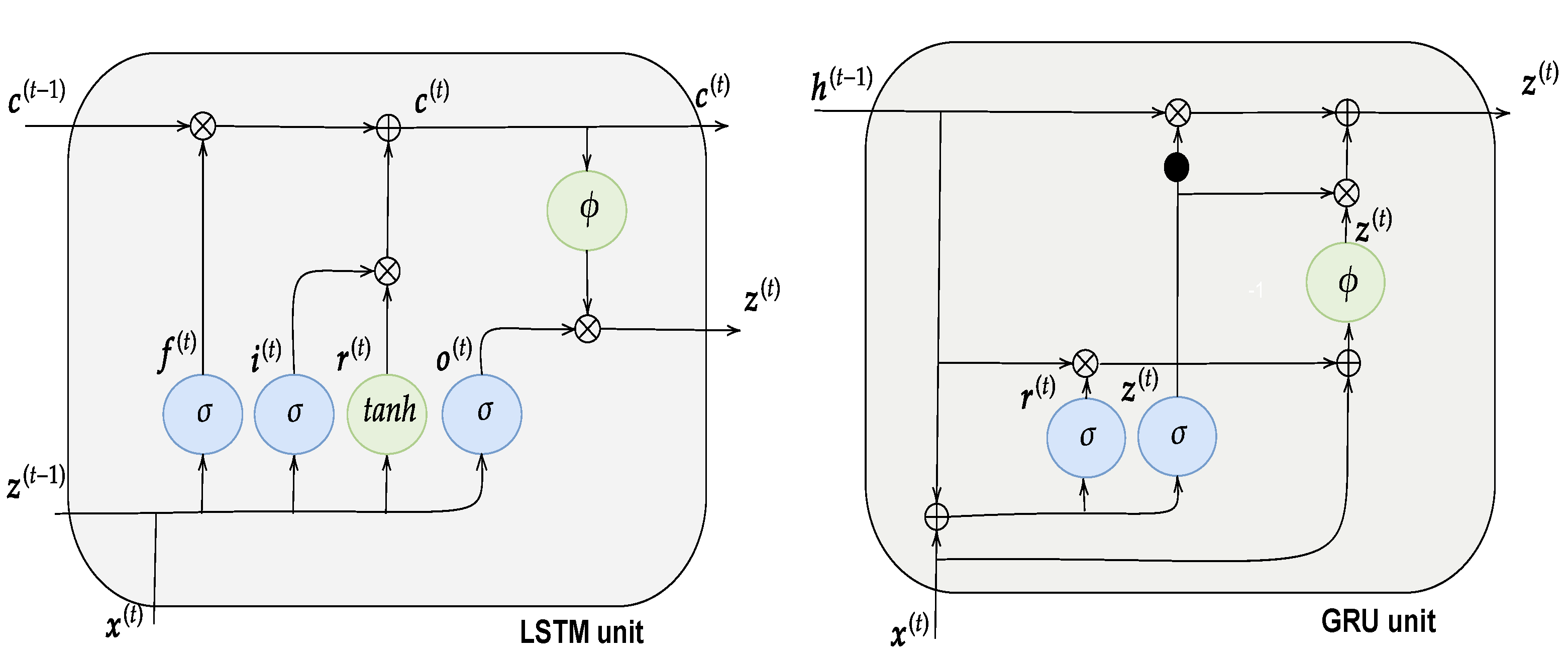
3.1.4. Long Short-Term Networks
3.1.5. Gated Recurrent Unit Networks
3.1.6. Convolutional Neural Networks
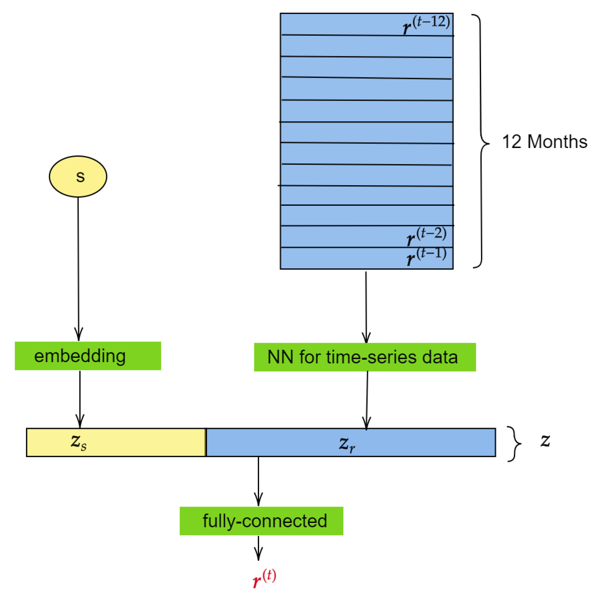
3.2. The Model
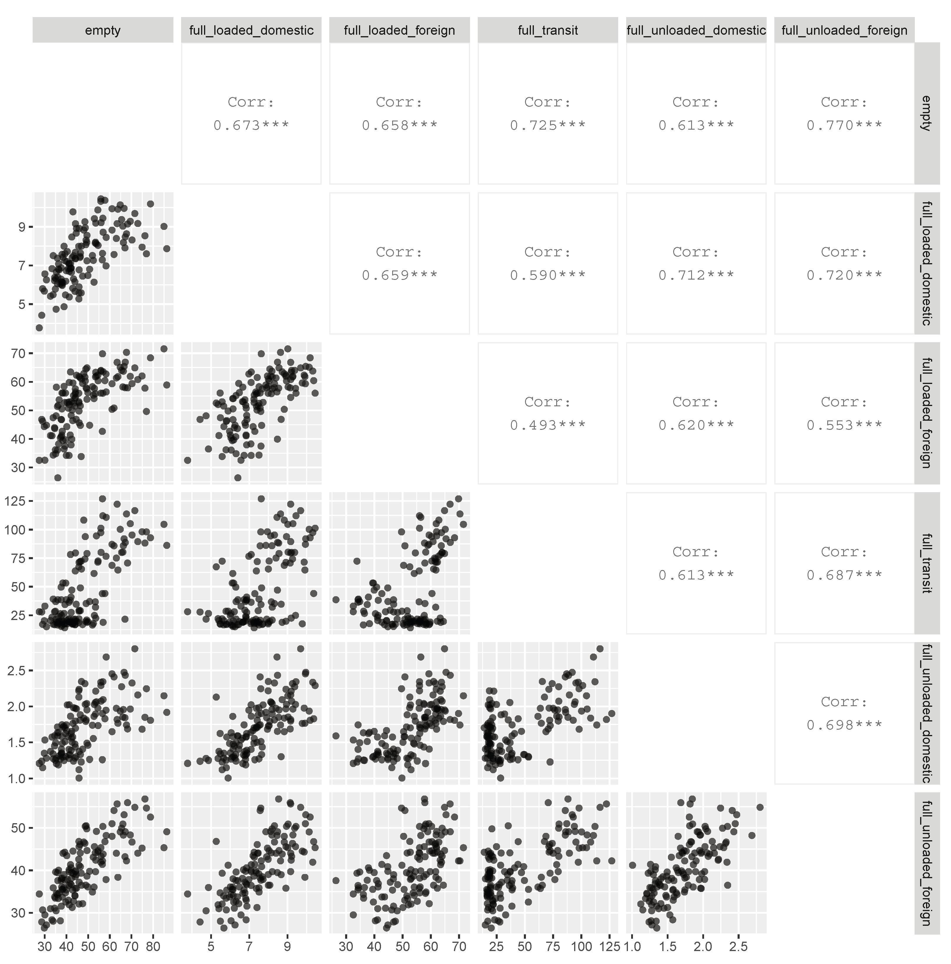
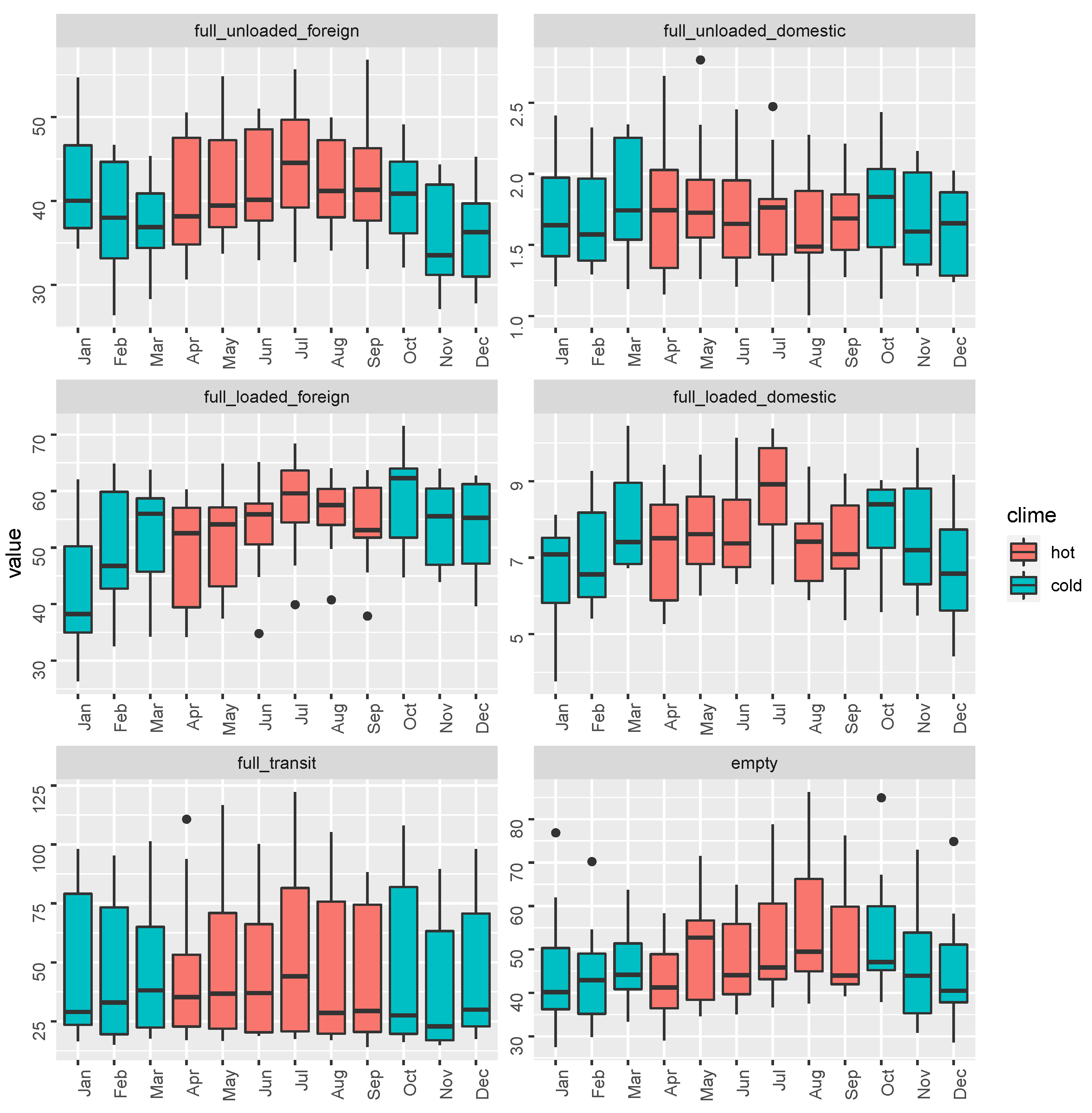
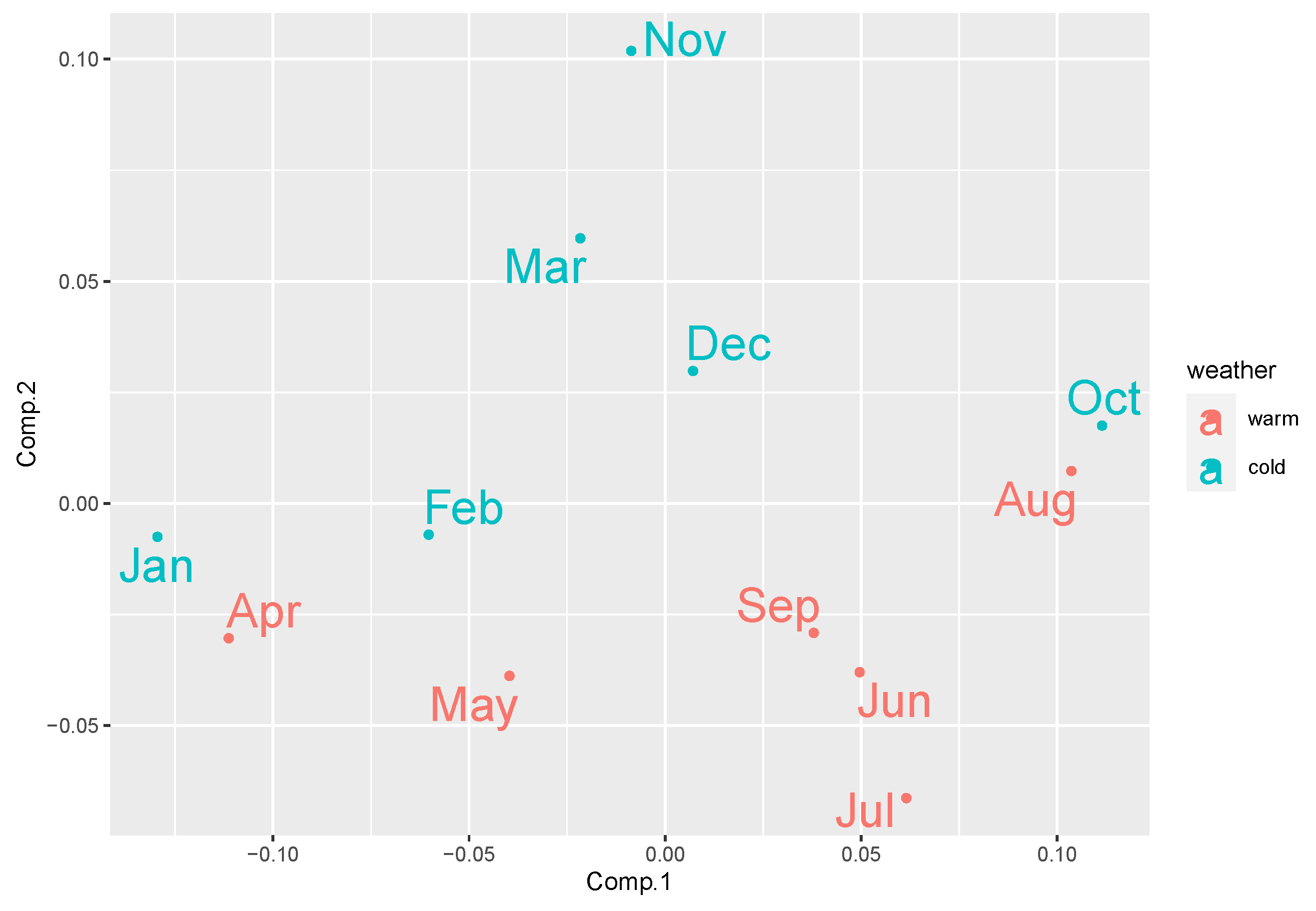
3.3. Data
4. Results
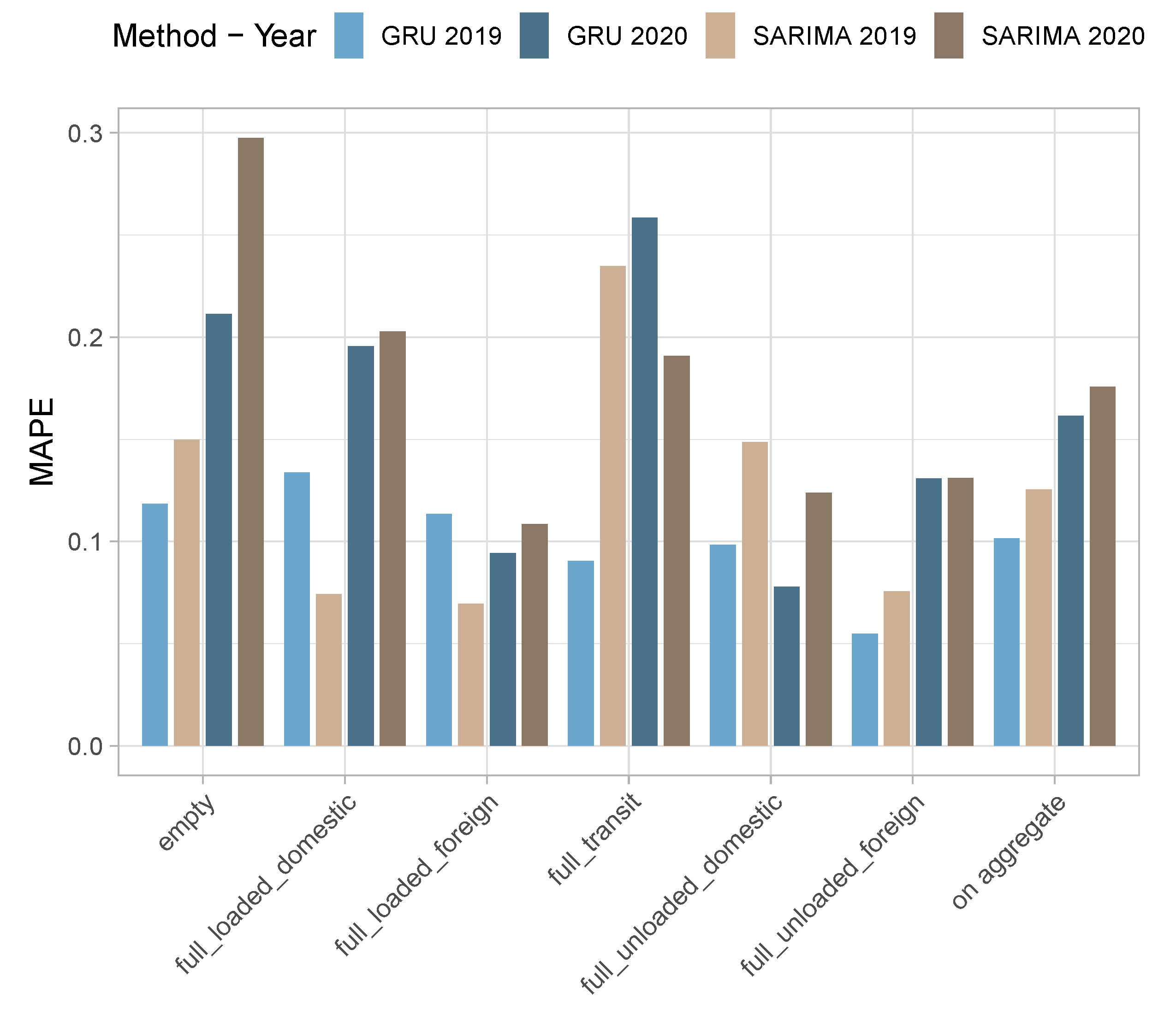
- In the first scenario, the models were calibrated using data up to December 2018, and forecasts were made for the calendar year 2019. In other words, data were partitioned in the training set, including data related to (from January 2010 to December 2018) and a testing set (from January 2019 to December 2019) for measuring the out-of-sample performance.
- In the second scenario, the models were calibrated using data up to December 2019, and forecasts were made for the calendar year 2020. In this case, we defined the training set and testing set as (from January 2010 to December 2019) and (from January 2020 to December 2020), respectively.
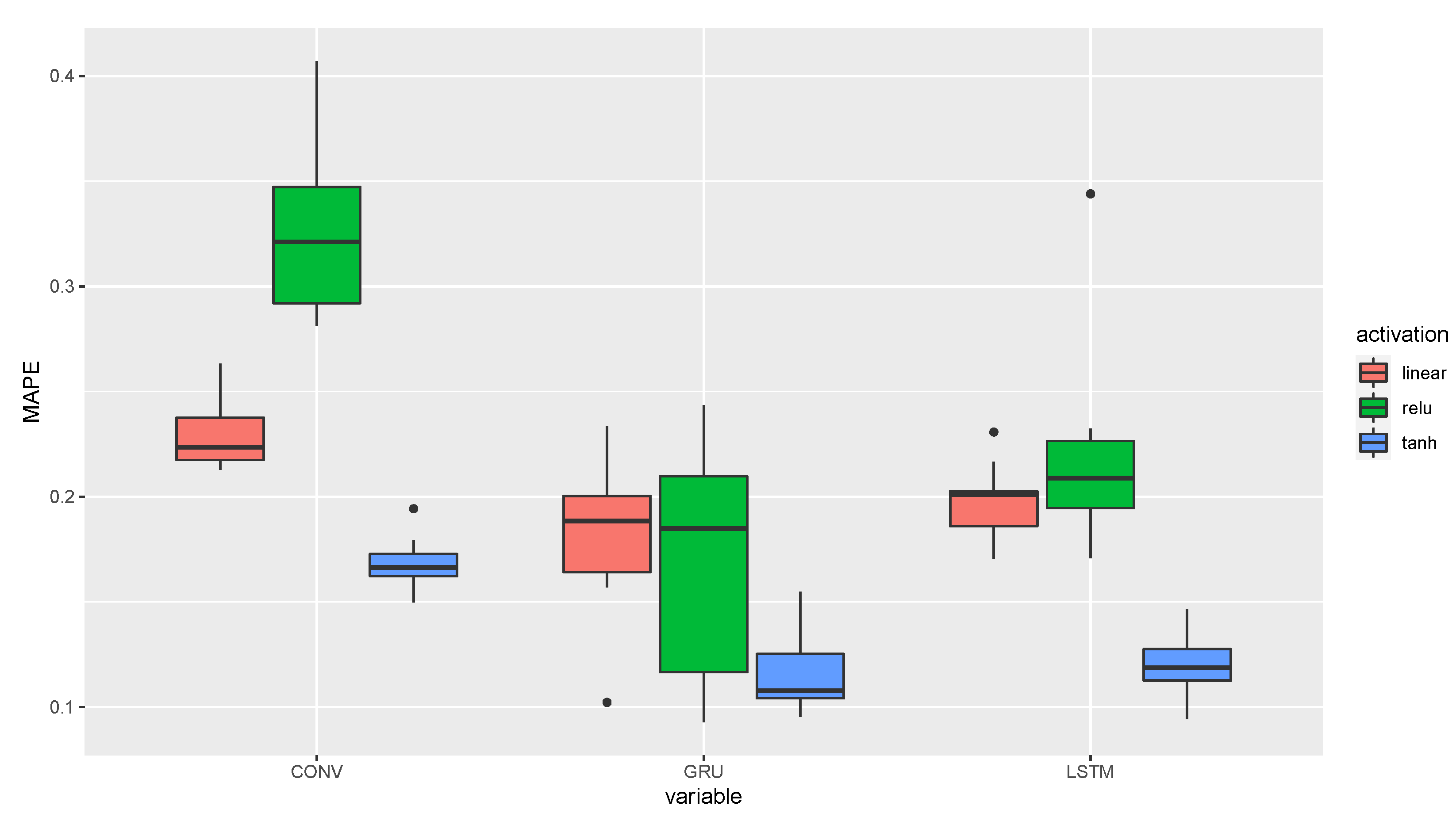
- The linear activation ;
- The tanh ;
- The relu function .
5. Conclusions
Author Contributions
Funding
Data Availability Statement
Conflicts of Interest
Abbreviations
| AIC | Akaike information criterion |
| ANN | Artificial neural network |
| ARIMA | Autoregressive integrated moving average |
| CNN | Convolutional neural network |
| GRU | Gated recurrent unit |
| LSTM | Long short-term memory |
| RNN | Recurrent neural network |
| TEU | Twenty-foot equivalent unit |
References
- Petering, M.E. Effect of block width and storage yard layout on marine container terminal performance. Transp. Res. Part E Logist. Transp. Rev. 2009, 45, 591–610. [Google Scholar] [CrossRef]
- Coto-Millán, P.; Baños-Pino, J.; Castro, J.V. Determinants of the demand for maritime imports and exports. Transp. Res. Part E Logist. Transp. Rev. 2005, 41, 357–372. [Google Scholar] [CrossRef]
- Cullinane, K.; Wang, T.F.; Song, D.W.; Ji, P. The technical efficiency of container ports: Comparing data envelopment analysis and stochastic frontier analysis. Transp. Res. Part A Policy Pract. 2006, 40, 354–374. [Google Scholar] [CrossRef]
- Parola, F.; Risitano, M.; Ferretti, M.; Panetti, E. The drivers of port competitiveness: A critical review. Transp. Rev. 2017, 37, 116–138. [Google Scholar] [CrossRef]
- Parola, F.; Notteboom, T.; Satta, G.; Rodrigue, J.P. Analysis of factors underlying foreign entry strategies of terminal operators in container ports. J. Transp. Geogr. 2013, 33, 72–84. [Google Scholar] [CrossRef]
- Parola, F.; Satta, G.; Panayides, P.M. Corporate strategies and profitability of maritime logistics firms. Marit. Econ. Logist. 2015, 17, 52–78. [Google Scholar] [CrossRef]
- Haralambides, H.E. Gigantism in container shipping, ports and global logistics: A time-lapse into the future. Marit. Econ. Logist. 2019, 21, 1–60. [Google Scholar] [CrossRef]
- Notteboom, T.; Pallis, A.; Rodrigue, J.P. Port Economics. In Management and Policy; Routledge: New York, NY, USA, 2020. [Google Scholar]
- Chu, C.Y.; Huang, W.C. Determining container terminal capacity on the basis of an adopted yard handling system. Transp. Rev. 2005, 25, 181–199. [Google Scholar] [CrossRef]
- Gharehgozli, A.; Zaerpour, N.; de Koster, R. Container terminal layout design: Transition and future. Marit. Econ. Logist. 2019, 22, 610–639. [Google Scholar] [CrossRef]
- Yap, W.Y.; Lam, J.S. Competition dynamics between container ports in East Asia. Transp. Res. Part A Policy Pract. 2006, 40, 35–51. [Google Scholar] [CrossRef]
- Anderson, C.M.; Opaluch, J.J.; Grigalunas, T.A. The demand for import services at US container ports. Marit. Econ. Logist. 2009, 11, 156–185. [Google Scholar] [CrossRef]
- Tavasszy, L.; Minderhoud, M.; Perrin, J.F.; Notteboom, T. A strategic network choice model for global container flows: Specification, estimation and application. J. Transp. Geogr. 2011, 19, 1163–1172. [Google Scholar] [CrossRef]
- Yap, W.Y.; Loh, H.S. Next generation mega container ports: Implications of traffic composition on sea space demand. Marit. Policy Manag. 2019, 46, 687–700. [Google Scholar] [CrossRef]
- Fung, M.K. Forecasting Hong Kong’s container throughput: An error-correction model. J. Forecast. 2002, 21, 69–80. [Google Scholar] [CrossRef]
- Verhoeven, P. A review of port authority functions: Towards a renaissance? Marit. Policy Manag. 2010, 37, 247–270. [Google Scholar] [CrossRef]
- Franc, P.; Van der Horst, M. Understanding hinterland service integration by shipping lines and terminal operators: A theoretical and empirical analysis. J. Transp. Geogr. 2010, 18, 557–566. [Google Scholar] [CrossRef]
- Zhu, S.; Zheng, S.; Ge, Y.E.; Fu, X.; Sampaio, B.; Jiang, C. Vertical integration and its implications to port expansion. Marit. Policy Manag. 2019, 46, 920–938. [Google Scholar] [CrossRef]
- Ferretti, M.; Parola, F.; Risitano, M.; Vitiello, I. Planning and concession management under port co-operation schemes: A multiple case study of Italian port mergers. Res. Transp. Bus. Manag. 2018, 26, 5–13. [Google Scholar] [CrossRef]
- Parola, F.; Pallis, A.A.; Risitano, M.; Ferretti, M. Marketing strategies of Port Authorities: A multi-dimensional theorisation. Transp. Res. Part A Policy Pract. 2018, 111, 199–212. [Google Scholar] [CrossRef]
- Mandják, T.; Lavissière, A.; Hofmann, J.; Bouchery, Y.; Lavissière, M.C.; Faury, O.; Sohier, R. Port marketing from a multidisciplinary perspective: A systematic literature review and lexicometric analysis. Transp. Policy 2019, 84, 50–72. [Google Scholar] [CrossRef]
- Kaliszewski, A.; Kozlowski, A.; Dkabrowski, J.; Klimek, H. Key factors of container port competitiveness: A global shipping lines perspective. Mar. Policy 2020, 117, 103896. [Google Scholar] [CrossRef]
- Castellano, R.; Fiore, U.; Musella, G.; Perla, F.; Punzo, G.; Risitano, M.; Sorrentino, A.; Zanetti, P. Do Digital and Communication Technologies Improve Smart Ports? A Fuzzy DEA Approach. IEEE Trans. Ind. Inform. 2019, 15, 5674–5681. [Google Scholar] [CrossRef]
- Molavi, A.; Lim, G.J.; Race, B. A framework for building a smart port and smart port index. Int. J. Sustain. Transp. 2020, 14, 686–700. [Google Scholar] [CrossRef]
- Ferretti, M.; Parmentola, A.; Parola, F.; Risitano, M. Strategic monitoring of port authorities activities: Proposal of a multi-dimensional digital dashboard. Prod. Plan. Control 2017, 28, 1354–1364. [Google Scholar] [CrossRef]
- Nikolopoulos, K.; Punia, S.; Schäfers, A.; Tsinopoulos, C.; Vasilakis, C. Forecasting and planning during a pandemic: COVID-19 growth rates, supply chain disruptions, and governmental decisions. Eur. J. Oper. Res. 2021, 290, 99–115. [Google Scholar] [CrossRef] [PubMed]
- Box, G.E.; Jenkins, G.M.; Reinsel, G.C.; Ljung, G.M. Time Series Analysis: Forecasting and Control; John Wiley & Sons: Hoboken, NJ, USA, 2015. [Google Scholar]
- Chan, H.K.; Xu, S.; Qi, X. A comparison of time series methods for forecasting container throughput. Int. J. Logist. Res. Appl. 2019, 22, 294–303. [Google Scholar] [CrossRef]
- Peng, W.Y. The comparison of the seasonal forecasting models: A study on the prediction of imported container volume for international container ports in Taiwan. Marit. Q. 2006, 25, 21–36. [Google Scholar]
- Peng, W.Y.; Chu, C.W. A comparison of univariate methods for forecasting container throughput volumes. Math. Comput. Model. 2009, 50, 1045–1057. [Google Scholar] [CrossRef]
- Schulze, P.M.; Prinz, A. Forecasting container transshipment in Germany. Appl. Econ. 2009, 41, 2809–2815. [Google Scholar] [CrossRef]
- Goodfellow, I.; Bengio, Y.; Courville, A.; Bengio, Y. Deep Learning; MIT Press Cambridge: Cambridge, MA, USA, 2016; Volume 1. [Google Scholar]
- Vapnik, V. The Nature of Statistical Learning Theory; Springer Science & Business Media: Berlin/Heidelberg, Germany, 2013. [Google Scholar]
- Wang, Y.; Meng, Q. Integrated method for forecasting container slot booking in intercontinental liner shipping service. Flex. Serv. Manuf. J. 2019, 31, 653–674. [Google Scholar] [CrossRef]
- Chen, Y.; Liu, B. Forecasting Port Cargo Throughput Based on Grey Wave Forecasting Model with Generalized Contour Lines. J. Grey Syst. 2017, 29, 51. [Google Scholar]
- Barua, L.; Zou, B.; Zhou, Y. Machine learning for international freight transportation management: A comprehensive review. Res. Transp. Bus. Manag. 2020, 34, 100453. [Google Scholar] [CrossRef]
- Wei, C.; Yang, Y. A study on transit containers forecast in Kaohsiung port: Applying artificial neural networks to evaluating input variables. J. Chin. Inst. Transp. 1999, 11, 1–20. [Google Scholar]
- Gosasang, V.; Chandraprakaikul, W.; Kiattisin, S. A comparison of traditional and neural networks forecasting techniques for container throughput at Bangkok port. Asian J. Shipp. Logist. 2011, 27, 463–482. [Google Scholar] [CrossRef]
- Milenković, M.; Milosavljevic, N.; Bojović, N.; Val, S. Container flow forecasting through neural networks based on metaheuristics. Oper. Res. 2021, 21, 965–997. [Google Scholar] [CrossRef]
- Xie, G.; Wang, S.; Zhao, Y.; Lai, K.K. Hybrid approaches based on LSSVR model for container throughput forecasting: A comparative study. Appl. Soft Comput. 2013, 13, 2232–2241. [Google Scholar] [CrossRef]
- Wang, G.; Ledwoch, A.; Hasani, R.M.; Grosu, R.; Brintrup, A. A generative neural network model for the quality prediction of work in progress products. Appl. Soft Comput. 2019, 85, 105683. [Google Scholar] [CrossRef]
- Zhou, X.; Dong, P.; Xing, J.; Sun, P. Learning dynamic factors to improve the accuracy of bus arrival time prediction via a recurrent neural network. Future Internet 2019, 11, 247. [Google Scholar] [CrossRef]
- Du, P.; Wang, J.; Yang, W.; Niu, T. Container throughput forecasting using a novel hybrid learning method with error correction strategy. Knowl.-Based Syst. 2019, 182, 104853. [Google Scholar] [CrossRef]
- Shankar, S.; Ilavarasan, P.V.; Punia, S.; Singh, S.P. Forecasting container throughput with long short-term memory networks. Ind. Manag. Data Syst. 2019, 120, 425–441. [Google Scholar] [CrossRef]
- Elman, J.L. Finding structure in time. Cogn. Sci. 1990, 14, 179–211. [Google Scholar] [CrossRef]
- Hochreiter, S.; Schmidhuber, J. Long short-term memory. Neural Comput. 1997, 9, 1735–1780. [Google Scholar] [CrossRef] [PubMed]
- Gers, F.A.; Schmidhuber, J.; Cummins, F. Learning to Forget: Continual Prediction with LSTM. Neural Comput. 2000, 12, 2451–2471. [Google Scholar] [CrossRef]
- Graziani, S.; Xibilia, M.G. Innovative Topologies and Algorithms for Neural Networks. Future Internet 2020, 12, 117. [Google Scholar] [CrossRef]
- Bengio, Y.; Ducharme, R.; Vincent, P. A Neural Probabilistic Language Model. Available online: https://proceedings.neurips.cc/paper/2000/file/728f206c2a01bf572b5940d7d9a8fa4c-Paper.pdf (accessed on 19 June 2022).
- Guo, C.; Berkhahn, F. Entity embeddings of categorical variables. arXiv 2016, arXiv:1604.06737. [Google Scholar]
- Sermpinis, G.; Karathanasopoulos, A.; Rosillo, R.; de la Fuente, D. Neural networks in financial trading. Ann. Oper. Res. 2019, 297, 293–308. [Google Scholar] [CrossRef]
- Kumar, A.; Singh, J.P.; Dwivedi, Y.K.; Rana, N.P. A deep multi-modal neural network for informative Twitter content classification during emergencies. Ann. Oper. Res. 2020, 1–32. [Google Scholar] [CrossRef]
- Greff, K.; Srivastava, R.K.; Koutník, J.; Steunebrink, B.R.; Schmidhuber, J. LSTM: A search space odyssey. IEEE Trans. Neural Netw. Learn. Syst. 2016, 28, 2222–2232. [Google Scholar] [CrossRef]
- Cho, K.; Van Merriënboer, B.; Gulcehre, C.; Bahdanau, D.; Bougares, F.; Schwenk, H.; Bengio, Y. Learning phrase representations using RNN encoder-decoder for statistical machine translation. arXiv 2014, arXiv:1406.1078. [Google Scholar]
- LeCun, Y.; Boser, B.E.; Denker, J.S.; Henderson, D.; Howard, R.E.; Hubbard, W.E.; Jackel, L.D. Handwritten digit recognition with a back-propagation network. In Proceedings of the Advances in Neural Information Processing Systems, Denver, CO, USA, 26–29 November 1990; pp. 396–404. [Google Scholar]
- Hornik, K.; Stinchcombe, M.; White, H. Multilayer feedforward networks are universal approximators. Neural Netw. 1989, 2, 359–366. [Google Scholar] [CrossRef]
- Hyndman, R.J.; Khandakar, Y. Automatic Time Series for Forecasting: The Forecast Package for R; Number 6/07; Monash University, Department of Econometrics and Business Statistics: Melbourne, Australia, 2007. [Google Scholar]
- Kingma, D.P.; Ba, J. Adam: A method for stochastic optimization. arXiv 2014, arXiv:1412.6980. [Google Scholar]
- Hastie, T.; Tibshirani, R.; Friedman, J.H.; Friedman, J.H. The Elements of Statistical Learning: Data Mining, Inference, and Prediction; Springer: Berlin/Heidelberg, Germany, 2009; Volume 2. [Google Scholar]


| Type | Mean | CoV | Min | Max | Range |
|---|---|---|---|---|---|
| empty | 48.3668 | 0.2611 | 27.5010 | 86.2680 | 58.7670 |
| full loaded domestic | 7.5032 | 0.1888 | 3.7720 | 10.4460 | 6.6740 |
| full loaded foreign | 52.8784 | 0.1842 | 26.3830 | 71.5410 | 45.1580 |
| full transit | 47.7746 | 0.6771 | 14.0320 | 126.9690 | 112.9370 |
| full unloaded domestic | 1.7183 | 0.2168 | 1.0070 | 2.8020 | 1.7950 |
| full unloaded foreign | 40.4105 | 0.1722 | 26.4280 | 56.8010 | 30.3730 |
| Non-Sesonal Orders | Sesonal Orders | |||||||
|---|---|---|---|---|---|---|---|---|
| Type | AR | I | MA | AR | I | MA | AIC | |
| 2019 Forecasts | full unloaded foreign | 0 | 1 | 2 | 0 | 1 | 1 | 477.7100 |
| full unloaded domestic | 0 | 1 | 2 | 0 | 0 | 0 | −73.9716 | |
| full loaded foreign | 5 | 1 | 0 | 1 | 0 | 1 | 648.0511 | |
| full loaded domestic | 2 | 1 | 0 | 1 | 0 | 0 | 224.9120 | |
| full transit | 0 | 1 | 1 | 0 | 0 | 2 | 792.7719 | |
| empty | 1 | 1 | 1 | 2 | 0 | 0 | 713.5212 | |
| 2020 Forecasts | full unloaded foreign | 0 | 1 | 2 | 1 | 1 | 2 | 540.6166 |
| full unloaded domestic | 0 | 1 | 1 | 0 | 0 | 1 | −58.0310 | |
| full loaded foreign | 0 | 1 | 2 | 0 | 0 | 2 | 717.8455 | |
| full loaded domestic | 1 | 1 | 1 | 1 | 0 | 0 | 252.6635 | |
| full transit | 0 | 1 | 1 | 1 | 0 | 0 | 882.7890 | |
| empty | 1 | 1 | 1 | 2 | 0 | 0 | 794.4201 | |
| Type | SARIMA | CONV | LSTM | GRU | |
|---|---|---|---|---|---|
| 2019 Forecasts | empty | 14.97% | 19.94% | 9.51% | 11.83% |
| full loaded domestic | 7.43% | 8.62% | 11.27% | 13.37% | |
| full loaded foreign | 6.96% | 8.00% | 8.19% | 11.34% | |
| full transit | 23.48% | 9.10% | 10.14% | 9.05% | |
| full unloaded domestic | 14.86% | 42.85% | 11.99% | 9.83% | |
| full unloaded foreign | 7.56% | 7.27% | 6.27% | 5.49% | |
| on aggregate | 12.54% | 15.96% | 9.56% | 10.15% | |
| 2020 Forecasts | empty | 29.75% | 19.51% | 22.09% | 21.13% |
| full loaded domestic | 20.28% | 14.48% | 19.60% | 19.55% | |
| full loaded foreign | 10.84% | 10.58% | 8.72% | 9.43% | |
| full transit | 19.08% | 23.45% | 28.42% | 25.85% | |
| full unloaded domestic | 12.39% | 43.13% | 9.36% | 7.79% | |
| full unloaded foreign | 13.10% | 11.79% | 14.46% | 13.09% | |
| on aggregate | 17.57% | 20.49% | 17.11% | 16.14% |
Publisher’s Note: MDPI stays neutral with regard to jurisdictional claims in published maps and institutional affiliations. |
© 2022 by the authors. Licensee MDPI, Basel, Switzerland. This article is an open access article distributed under the terms and conditions of the Creative Commons Attribution (CC BY) license (https://creativecommons.org/licenses/by/4.0/).
Share and Cite
Ferretti, M.; Fiore, U.; Perla, F.; Risitano, M.; Scognamiglio, S. Deep Learning Forecasting for Supporting Terminal Operators in Port Business Development. Future Internet 2022, 14, 221. https://doi.org/10.3390/fi14080221
Ferretti M, Fiore U, Perla F, Risitano M, Scognamiglio S. Deep Learning Forecasting for Supporting Terminal Operators in Port Business Development. Future Internet. 2022; 14(8):221. https://doi.org/10.3390/fi14080221
Chicago/Turabian StyleFerretti, Marco, Ugo Fiore, Francesca Perla, Marcello Risitano, and Salvatore Scognamiglio. 2022. "Deep Learning Forecasting for Supporting Terminal Operators in Port Business Development" Future Internet 14, no. 8: 221. https://doi.org/10.3390/fi14080221
APA StyleFerretti, M., Fiore, U., Perla, F., Risitano, M., & Scognamiglio, S. (2022). Deep Learning Forecasting for Supporting Terminal Operators in Port Business Development. Future Internet, 14(8), 221. https://doi.org/10.3390/fi14080221