Exploring Distributed Deep Learning Inference Using Raspberry Pi Spark Cluster

Abstract

Raspberry Pi (Pi) is a versatile general-purpose embedded computing device that can be used for both machine learning (ML) and deep learning (DL) inference applications such as face detection. This study trials the use of a Pi Spark cluster for distributed inference in TensorFlow. Specifically, it investigates the performance difference between a 2-node Pi 4B Spark cluster and other systems, including a single Pi 4B and a mid-end desktop computer. Enhancements for the Pi 4B were studied and compared against the Spark cluster to identify the more effective method in increasing the Pi 4B’s DL performance. Three experiments involving DL inference, which in turn involve image classification and face detection tasks, were carried out. Results showed that enhancing the Pi 4B was faster than using a cluster as there was no significant performance difference between using the cluster and a single Pi 4B. The difference between the mid-end computer and a single Pi 4B was between 6 and 15 times in the experiments. In the meantime, enhancing the Pi 4B is the more effective approach for increasing the DL performance, and more work needs to be done for scalable distributed DL inference to eventuate.

1. Introduction

Machine learning (ML) is consistently one of the most-applied computing disciplines in the current technological era and has become the norm synonymous with artificial intelligence (AI). The popularity of ML and its widespread use in many applications has led it to become a must for every business or organization intending to gain an edge over their competitors. Deep learning (DL) is a subset of ML. The differentiation between the two lies in the number of layers in the architecture of artificial neural networks. A deep neural network has more than one hidden layer. Contrariwise, an artificial neural network like Support Vector Machine (SVM) has only one hidden layer [1]. DL has seen steady adoption because of its performance over traditional state-of-the-art ML algorithms used in different fields, particularly image processing [2,3]. A popular example of a DL framework is TensorFlow, which has support for scalability in training DL models in a distributed manner, capable of scaling across 200 workers [4]. However, the distributed inference aspect in TensorFlow has yet to be tested so far.

Nowadays, researchers no longer solely implement DL-based image processing on high-performance hardware. Researchers have experimented with low-cost, low-power embedded devices such as Raspberry Pi and Nvidia Jetson Nano. These include an AI traffic control system, face recognition systems, as well as an integrated smart CCTV system [5,6,7]. The computational power of Raspberry Pi was barely sufficient for training ML models. Some researchers have opted to use a pre-trained model that was trained using powerful hardware before deployment on Raspberry Pi [8]. Thus, Raspberry Pi is mostly limited to prototyping DL inference operations as an embedded device rather than training DL models.

Raspberry Pi (Pi) is a single-board computer (SBC) designed and manufactured by the Raspberry Pi Foundation in the United Kingdom. Compared to a standard mid-end desktop which typically costs around US$500 to US$600, the latest Pi 4 Model B (Pi 4B) costs just US$35 for the base 2 GB RAM model. Its low cost makes it appealing among IoT hobbyists and it is used for prototyping embedded systems in research. Pi 4B is powered by a Broadcom BCM2711 system-on-a-chip (SoC), comprising four Cortex-A72 cores at a clock speed of 1.5 GHz and two to eight gigabytes of LPDDR4-3200 RAM, depending on the model variant. In contrast to previous generations of Pi, Pi 4B includes the addition of two USB 3.0 ports which allow for faster forms of storage to be used, such as an external HDD or even an external SSD in place of the traditional microSD card. Pi 4B runs on its customized version of the Debian operating system named Raspberry Pi OS, even though it supports other Linux operating systems such as Ubuntu and Arch Linux ARM.

However, DL inference performance benchmarks for Pi 4B are lacking, as most research papers focus on prototyping AI systems using Pi 4B. This is especially important as Pi is increasingly replacing traditional computers in prototyping systems. The choice of choosing a base system for prototyping depends on the computational complexity of the prototype system itself. In a scenario where researchers plan to implement a prototype system, the choice for the base system would be rigorously evaluated to determine whether it fulfills the requirements set out for prototyping. As Pi 4B is touted to be faster than its predecessor, the performance gap between Pi and a conventional computer may be reduced. Most ML and DL benchmarks carried out with the previous generation of Pi (3B) could quickly become obsolete and irrelevant. Thus, there is a need to re-investigate the performance difference between Pi 4B and a conventional x86 desktop computer to ensure performance review results are up to date. There is also a need to study the improvement of the enhancements for Pi 4B in lessening the performance gap between Pi 4B and a conventional x86 desktop computer. Given its low cost, the increase in the competitiveness of the Pi 4B against powerful and modern hardware could also increase its appeal for prototyping.

Other than enhancing Pi’s performance through software tweaks, the clustering of multiple Pis is also known to improve performance in heavy processing workloads and offers somewhat competitive performance for certain workloads [9,10,11]. Despite the existence of the research mentioned in earlier papers implementing Pi clusters, there is very little to no information about the performance evaluation of Pi clusters in DL inference. This also forms another research gap to further investigate how well Pi SBCs perform in many aspects via system comparisons and scalability tests. To the best of the authors’ knowledge, the closest attempt to distributed DL inference was by using the Apache Spark clustering framework via Spark MLlib. However, this framework only encompasses traditional ML paradigms which limit flexibility in implementing the distributed DL system [12]. Such a limitation would disallow the implementation of novel, state-of-the-art DL models into a distributed system. For context, Apache Spark supports only a popular set of classification, regression, and clustering algorithms such as random forest and linear SVM. Its closest classifier is multilayer perceptron, though customizability is limited to the number of layers rather than the entire neural network structure.

Apache Spark is a data processing engine suite designed for distributed processing and data analytics. It is incorporated into the Hadoop ecosystem by working with or replacing Hadoop MapReduce. Intermediate operation results in Spark are stored as resilient distributed datasets (RDDs), which use RAM. By using RDDs, processing operations can be up to 100 times faster compared to MapReduce, as there are no intermediate disk I/O operations that limit the processing speed. However, this comes at the cost of memory space for Spark jobs, which necessitates the use of high-capacity RAM. While the impact of using a Spark cluster for inference tasks in MLlib is already known, as seen in [12], there is no information on the impact of using a Spark cluster for distributed inference in other DL frameworks outside MLlib. DL frameworks, such as TensorFlow and PyTorch, offer superior versatility and customizability regarding the creation and testing of a DL model. Moreover, MLlib is concerned with traditional ML paradigms and not DL, as per the focus of this paper. Thus, there is a need to investigate the performance difference between using a Spark cluster versus a single system for inference tasks outside of the MLlib framework.

To reiterate, the entire scope of this paper first encompasses the study on the effectiveness of distributed inference using Spark TensorFlow Distributor, which is achieved by investigating the performance difference between using a single Pi and a 2-node Pi cluster. Identifying the performance difference between a single system and a 2-node cluster is crucial in understanding the effectiveness of distributed inference versus a single system, as the relatively novel Spark TensorFlow Distributor is experimentally trialed for this study as opposed to Spark MLlib which is proven to scale in ML tasks. So far, Spark MLlib remains in use as the preferred option for scalable ML with the Spark clustering framework and it is interesting to know whether distributed DL inference with Spark TensorFlow Distributor would show potential to compete against MLlib not just in the customizability aspect, but also in terms of performance scalability. Second, the performance gap between Pi 4B and a standard mid-end desktop in inference tasks involving lightweight and standard DL models will be identified. In contrast to standard DL models, lightweight models require significantly less processing power for inference, which is suitable for resource-constrained systems. However, these models are less accurate than their novel DL counterparts in most tasks. In the interest of fairness, both lightweight and standard DL models are included to investigate the performance gap between the two systems. In addition, this comparison may help discover a relationship between using lightweight or standard DL models. Through the identification of the performance gap, an estimation of Pi 4B’s DL performance can be made for reference when setting up DL prototype systems using Pi 4B. Third, the performance of the enhanced Pi 4B will be studied and compared against the standard unaltered Pi 4B and its 2-node Spark cluster counterpart in TensorFlow inference tasks. This aspect evaluates the impact of the enhancements on the Pi 4B and determines the more effective approach to increasing the DL performance of the Pi 4B. So far, TensorFlow is the only DL library that officially supports the Spark clustering framework via Spark TensorFlow Distributor for scalable DL. The use of TensorFlow Lite for this study was originally considered, but it was revealed that the Spark TensorFlow Distributor, which interfaces both Spark and TensorFlow, only supports the standard version of TensorFlow. Thus, it was not possible to use TensorFlow Lite with Spark TensorFlow Distributor.

The rest of the paper is organized as follows. Section 2 presents the related work that serves as motivation to investigate the DL performance of the Pi 4B, distributed or otherwise. Section 3 presents the evaluation metrics used, the procedure of the experiments, environment configuration, test systems, software used for carrying out the experiments of this study, and the implementation of the Spark cluster. Section 4 details the experimental results and the results of the enhanced Pi. Section 5 discusses the results and hypotheses and the performance gap of the Pi 4B relative to other systems. Section 6 details the contribution and suggestions of this work, as well as possible future works.

2. Related Work

2.1. DL Inference on Pi

DL on Pi is a recently explored field. As seen in [13], a performance review involving an NVIDIA Jetson TX2, NVIDIA Jetson Nano, and Pi 4B in DL workloads was carried out. The results of the study have shown that the Pi 4B took between 5 times and 9 times longer than the Nano and the TX2 in executing inference on datasets while accuracy remained similar with a deviation of 3%. The authors stated that even though Pi is the most cost-effective hardware of the three, the lack of DL acceleration makes it unfavorable for DL and AI. They concluded that “while the Jetson TX2 held the highest DL performance and bore the highest cost of the three SBCs, it is impossible to attain a highly performant SBC in DL with the price tag of a Pi at $35”.

In [14], an experiment for performance analysis of edge computing platforms which are intended to serve as backup systems for autonomous drones was carried out. The devices used for testing are a Pi 3B with 1 GB RAM, an Intel Neural Compute Stick (NCS) 2 AI accelerator, and a laptop PC powered by an Intel Core i5-8250U 4-core processor clocked at 1.6 GHz with 8 GB RAM. For their test, they tested three configurations: the Pi 3B with and without the NCS, and the laptop PC with the NCS. To test each configuration, they executed applications deemed to be safety critical in the backup system. The applications are Single Shot MultiBox Detector (SSD)-based image recognition, State Lattice Planner (SLP) for routing flight paths locally, and Pix2Pix (P2P) for generating an aerial image of the drone into a map image to function as a fail-operational alternative for GPS. While the results showed a tremendous speedup of 38.51 times when the Pi 3 was paired with the NCS for the SSD-based image recognition application, the difference in performance between the two Pi configurations (with and without NCS) for SLP and P2P was not apparent. However, since SSD is the only application using a single deep neural network in contrast to SLP and P2P, the use of a neural accelerator helps to increase the DL performance of the Pi in DL applications. Even with an AI accelerator, the Pi is not guaranteed to perform at the level of an x86 computer, as some applications in the experiment were not entirely dependent on AI and leaned more toward conventional processing workloads. Pi development boards, while being affordable, have a low-end System-on-a-Chip (SoC) that is not meant for extensive processing workloads such as model training. This was apparent when other researchers resorted to offloading model training tasks to a conventional computer, and the trained model was then moved to the Pi for inference as seen in [8]. The authors hypothesize that most applications are written for the x86 computer architecture and the lack of processing power and optimization for the ARM architecture results in a huge performance deficit between the two platforms.

2.2. Clustering with Multiple Pis

Outside of the ML/DL domain, other researchers have implemented Pi clusters to investigate whether these clusters would offer non-trivial performance comparable to that of server systems. Among the earliest attempts of benchmarking a Pi cluster in the last 5 years was that described in [15]. For their discovery, they connected twelve Pi 2 SBCs to a local networking switch, and the cluster is coordinated through Message Passing Interface (MPI) by using an implementation named MPICH. The results showed significant speedup with higher node count, though diminishing occurs with higher node count. The 12-node Pi 2 cluster only attained a speedup of 7.84 times over the single Pi 2. Regardless, their discovery proved that homogeneous clustering of Pi SBCs will improve computational performance. Unfortunately, there was no direct comparison made against modern computer hardware for the case of the 12-node Pi 2 cluster.

Another newer but similar outcome was found in [16] where a group of researchers set up a Hadoop cluster of ten Pi 3 SBCs against a mid-end desktop computer in their experiment to evaluate the performance of the Pi cluster. The desktop computer ran an Intel Core i5-4460 with 8 GB RAM. The authors stated that the relatively low-cost of Pi clusters and the scalability of the Hadoop ecosystem make these clusters usable for an array of heavy processing operations. In smaller datasets, the performance of a 10-node Pi cluster is 12.5 percent lower than the conventional x86 mid-end desktop computer in the experiment. However, the cluster was up to 20 percent faster in larger dataset sizes. Their findings suggest that the clustering of Pi units for big data processing may be a good idea to achieve similar processing performance as an x86 system at a lower cost.

The ARM hardware architecture powering the Pi has not seen use in high-performance computing (HPC) such as in servers. Rather, it is catered to low-power, portable devices like smartphones, tablets, and IoT devices which emphasize power efficiency rather than processing performance. The only recent attempt at clustering Pi 4B SBCs was done by a group of Greek researchers for evaluating Pi 4 cluster performance in tourism-related ML applications using Apache Spark [12]. Their results in [12] also showed diminishing returns with higher node counts, with 2 nodes providing the most significant speedup impact on the training and inference time. The researchers commented the cluster suffices for the training and the execution of ML models for edge computing and the performance evaluation of the cluster should be carried out with models of higher complexity. They also pointed out the need for testing with other DL libraries such as TensorFlow, which are suited for heavier processing workloads.

At the time of writing, no researchers are experimenting on a cluster of Pi 4B SBCs for DL to evaluate its performance compared to other hardware solutions. As per the discussions in [12], the authors suggested a more comprehensive performance evaluation involving modern DL libraries beyond Spark MLlib.

Table 1. Summary of research coverage from previous works regarding Pi DL inference and distributed Pi clusters.

Study	Pi Model	DL/ML	Clustering	Framework Used	Findings
[13]	4B	Yes	No	-	Pi 4B performs the worst in inference tests involving Jetson Nano and Jetson TX2 due to a lack of AI acceleration.
[14]	3B	Yes	No	-	Pi 3B with AI accelerator performs almost similarly to laptop computer in SSD, however it falls behind in SLP and P2P with a vast gap.
[15]	2	No	Yes	MPICH	Clustering of Pi improves performance, speedup factor diminishes with higher node count.
[16]	3	No	Yes	Apache Hadoop	Negligible improvement in low-processing workloads with clustering. The performance of 10-node cluster rivals conventional x86 desktop computer.
[12]	4B	Yes	Yes	Apache Spark	Model training time and test prediction time dropped sharply at 2 nodes, diminishes with higher counts.

summarizes the research papers relevant to this experimental study. Most of the DL-relevant papers have not explored clustering with Pi 4, and most clustering attempts listed in the table used implementations of MPI. These clustering attempts on Pi were quite outdated, as most of them used Pi 3 SBCs. Of all the research papers listed, only [12] used Pi 4 SBCs and Apache Spark as the distributed processing framework for the cluster. However, their experiment was concerned with distributed training and distributed inference using MLlib. With this in mind, the authors propose research that seeks to evaluate the performance of Pi 4 SBC(s) in distributed DL inference using TensorFlow and Apache Spark with the clear objective of evaluating the DL performance of the Pis in image processing-related DL workloads. Specifically, DL performance is evaluated on applications using a neural network model such as those for image classification and face detection.

3. Methodology

3.1. Evaluation Metrics

This section outlines and explores the performance metrics that were used for evaluation in the experiments. Most of the performance metrics are chosen from the research paper reviews in Section 2, though interpretations of the metrics may be different depending on the context of the research scope and objective.

The metrics chosen for the experiments are execution time, frames per second (FPS), and speedup. Their respective equations are shown in

Table 2. Evaluation metrics used in the experiments and their respective equations.

Evaluation Metrics	Equations
Execution Time [14,16,17]	$ET=T_e-T_s$ where $ET$ represents execution time, $T_e$ represents the end time of request, and $T_s$ represents the start time of request.
Frames Per Second (FPS) [18,19]	$FPS=\frac{N}{s}$ where $N$ represents the number of image frames rendered and $s$ represents one second.
Speedup [15,20]	$S_n=\frac{T_1}{T_n}$ where $S_n$ represents speedup in configuration n, $T_1$ represents execution time for the baseline configuration and $T_n$ represents the execution time in the configuration n

. Execution time is defined as “a period in which an event is actively operating” [17]. It is the time taken to complete an execution job. Execution time as a performance metric has been used in many papers involving processing applications, as with [14,16] reviewed earlier in Section 2. Execution time is used as the primary performance metric in this study because this metric well represents the real-world processing performance for an application or a system, as opposed to the theoretical on-paper performance measures such as GFLOPS. In this paper, this term is synonymous with model inference time.

The definition of frames per second is perhaps best defined as the number of image frames rendered in one second, which is commonly used for videos and for benchmarking graphics performance in video games. This is the case as videos are essentially a continuous sequence of image frames. However, there are multiple interpretations of this metric. For example, Ref. [18] defined it as the “measure of fluidness of movement”, as higher FPS relates to smoother and more fluid motion in videos and games alike. Instead of merely focusing on video camera fluidity and smoothness, FPS is also used as a metric for inference speed in object detection and recognition, especially in [19], where the authors benchmarked ZF’s in-house ProAI SBC against the NVIDIA Jetson Nano and a Dell laptop with a dedicated NVIDIA Quadro P2000 workstation GPU. This specific metric is used for the experiment where rendering frames that have undergone face detection highly depend on the inference speed of the face detection model, rather than the FPS as captured by the camera. For this study, the former is used since DL model inference related to face detection processes a series of frames that are captured by a source before being returned as another set of frames.

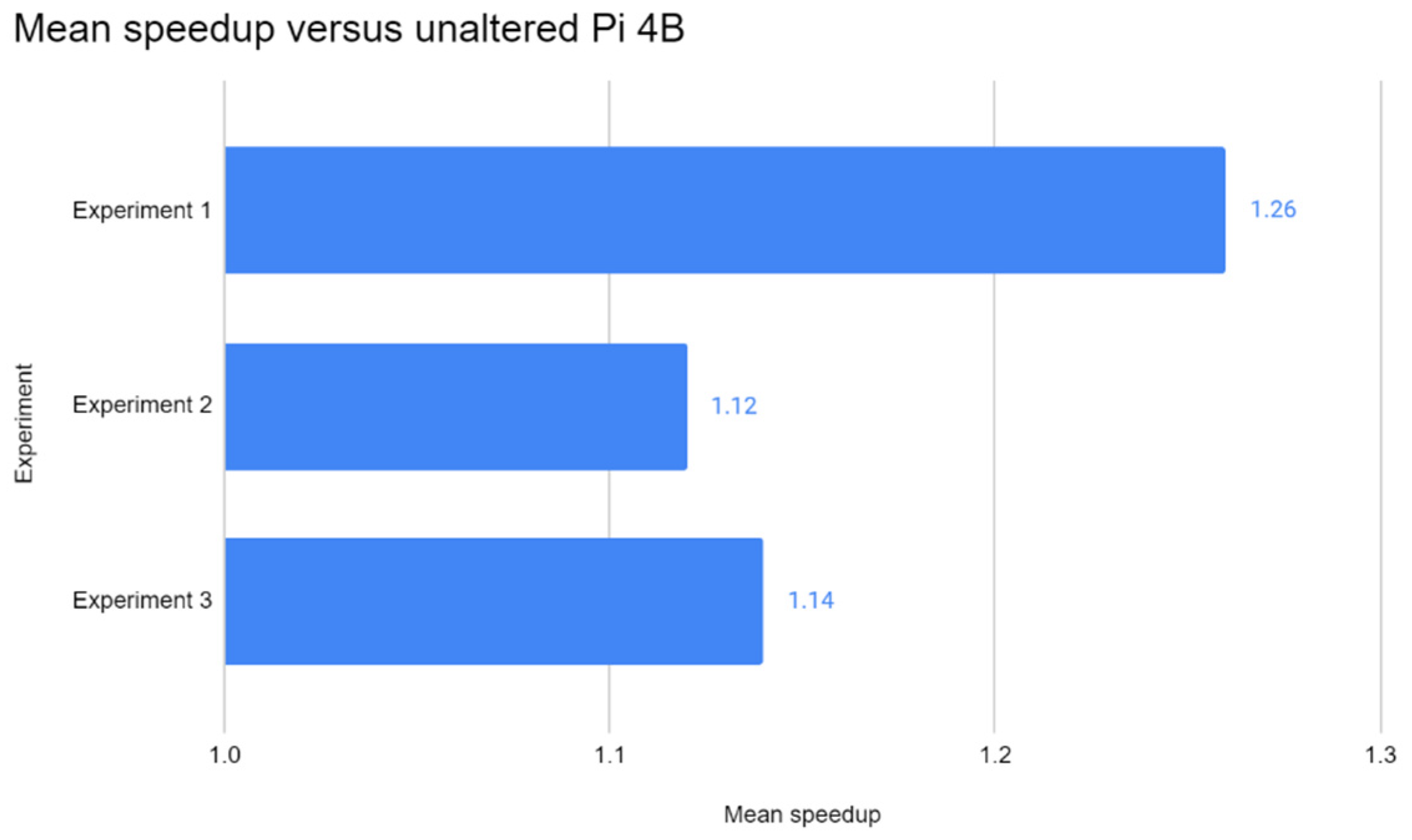
Speedup is defined as “the ratio of the performance improvement on different input sizes between two systems processing the same problem” [20]. Speedup is a metric used to measure the effectiveness of a configuration versus some baseline configuration for a processing job, as found in [15,20]. Besides being used in clustering versus single node scenarios, as per the case of Pi 4B versus the 2-node Pi 4B Spark cluster, it is also used for comparing the performance difference between different system configurations, processing models, and software settings. This specific metric is used for measuring the effectiveness of distributed inference using Spark TensorFlow Distributor, the effectiveness of the enhancements on the Pi, and the performance gap between systems, which are the scopes of this study.

3.2. Neural Network Models & Datasets Used

The first experiment used the ImageNetV2 [21] and CIFAR10 [22] datasets for evaluating the inference performance in image classification for every system stated in Section 3.6. ImageNetV2 was chosen as it is considered the benchmark dataset for classification models. CIFAR10 was chosen to complement it as a simpler and smaller dataset in contrast to the complex nature of ImageNetV2. The next experiment deals with face detection performance using the WIDER FACE [23] image dataset, which was the face detection benchmark dataset for the second experiment. Convolutional neural networks (CNN) such as Inceptionv3 and its lightweight counterpart, MobileNetV3, were used for image classification for all system configurations in the first experiment, whereas RetinaFace, YOLOface, and Multi-task Cascaded Convolutional Network (MTCNN) were used solely for face detection in the second and third experiments.

Nowadays, there are a wide variety of CNN architectures for different use cases. Newer CNN architectures can classify datasets with a high number of labels, such as ImageNet, at higher accuracy, as with InceptionV3. InceptionV3 is the newest version of the Inception neural network model and contains a different neural network structure as opposed to its predecessors. It is pre-trained on the ImageNet dataset, which saves the hassle of transfer learning, as inference can be done on the test set of the ImageNet dataset directly. It is one of the best image classification models in terms of accuracy and is therefore chosen for the experiment to investigate the performance trade-off for the testing accuracy gained. MTCNN [24], RetinaFace [25], and YOLOface [26] are other CNN architectures optimized for face detection. YOLOface is a version of the YOLOv3 CNN model trained on the WIDER FACE dataset, and it obtains higher accuracy than YOLOv3 in detecting faces. MTCNN is different and is comprised of 3 components. As explained in [27], the first component is the Proposal Network (P-Net) which generates candidate windows that help in classifying images as ‘face’ or a ‘non-face’. These candidate windows are used to estimate bounding boxes on face locations. The second component, the Refine Network (R-Net), is intended to reject false candidate windows. Finally, the Output Network (O-Net) outputs the facial landmarks’ positions based on the results of the two previous components. RetinaFace is a recent state-of-the-art face detection architecture that uses feature pyramid networks that are based on the concept of convolution seen in CNNs. Notably, it achieved one of the highest accuracies in the WIDER FACE dataset at 91.4%.

Table 3. Datasets and models used in Experiments 1 to 3.

Experiment	Datasets Used	Models Used
Experiment 1	ImageNetV2 [21], CIFAR10 [22]	InceptionV3, MobileNetV3
Experiment 2	WIDER FACE [23]	MTCNN [24], RetinaFace [25], YOLOface [26]
Experiment 3	-	MTCNN [24], RetinaFace [25], YOLOface [26]

summarizes the datasets and models used in Experiments 1 to 3. The use of common lightweight face detection models such as the Haar-Cascade algorithm and SSD for Experiments 2 and 3 was not considered, as the intended focus was solely on comparing state-of-the-art, high-accuracy face detection models on Pi against the rest of the system configurations for the coverage of this research.

For Experiment 1, the datasets used were the ImageNetV2 test set and the CIFAR10 test split. The ImageNetV2 dataset is a specialised test set that follows the original ImageNet2012 dataset with the same label space, each comprising 10 test images per class. It is comprised of 10,000 test images which can be paired with an existing model that is pre-trained on the ImageNet2012 dataset for running inference. The CIFAR10 test split is comprised of 10,000 images which are 32 × 32 in resolution and are coloured. For consistency reasons, test splits for these two datasets were chosen as the goal was to evaluate the performance across every system configuration rather than evaluating the neural network models used in this paper.

For Experiment 2, the WIDER FACE dataset [23], which is a face detection benchmark containing faces taken from the WIDER dataset, was used. The official recommended dataset split is 40% for training, 10% for validation, and 40% for testing. Its test split dataset contains 16,097 images, which are similar in size to the train split. Originally, the plan was to use the test split for executing inference on the WIDER FACE dataset. But during the experiment, the time taken was exorbitantly long for low-end devices where it required almost a week to complete inference on a single iteration on the Pi 4B. Hence, the decision was taken to reduce the dataset size to the validation split, which contained 3220 images.

For Experiment 3, the experiment captured frames continuously in a real-time face detection test.

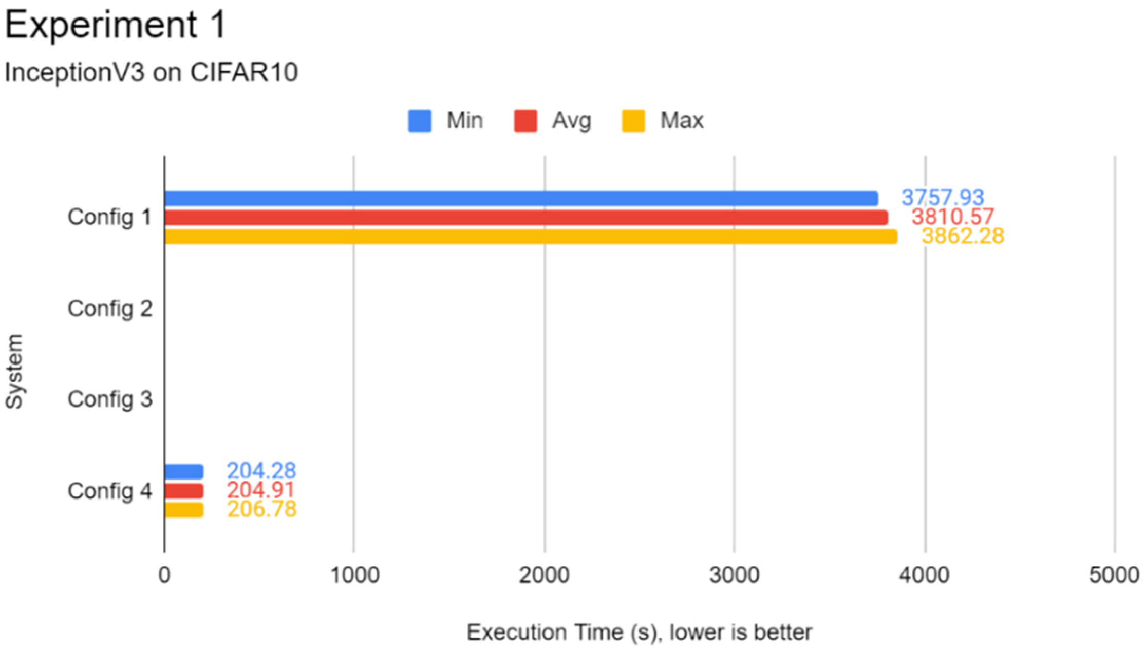
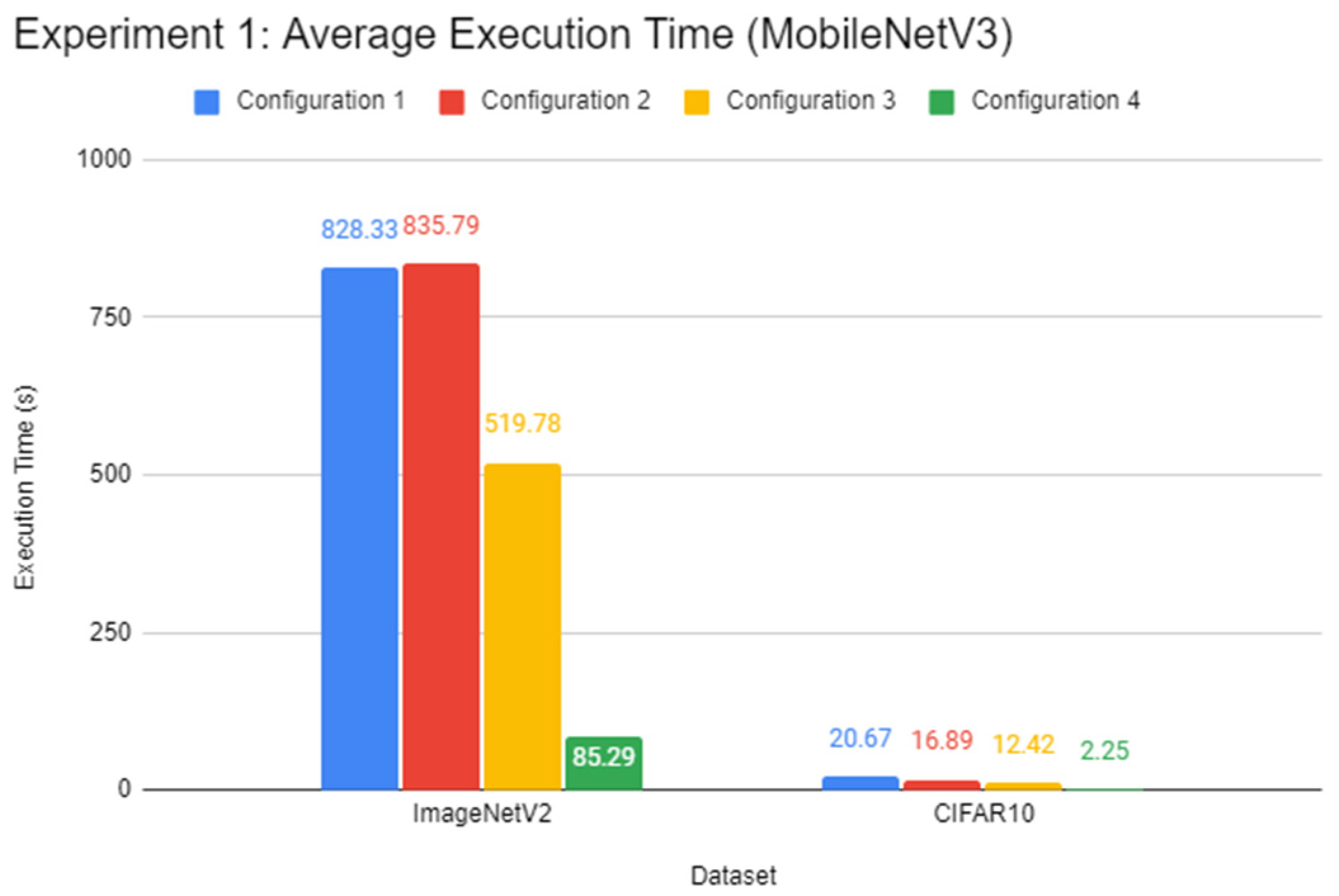
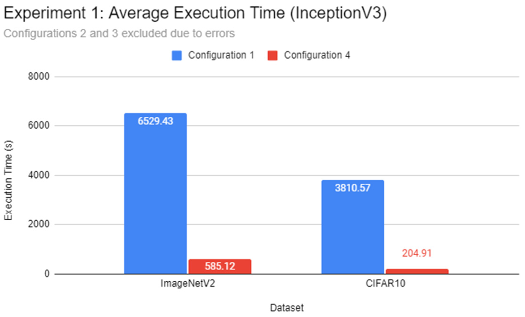
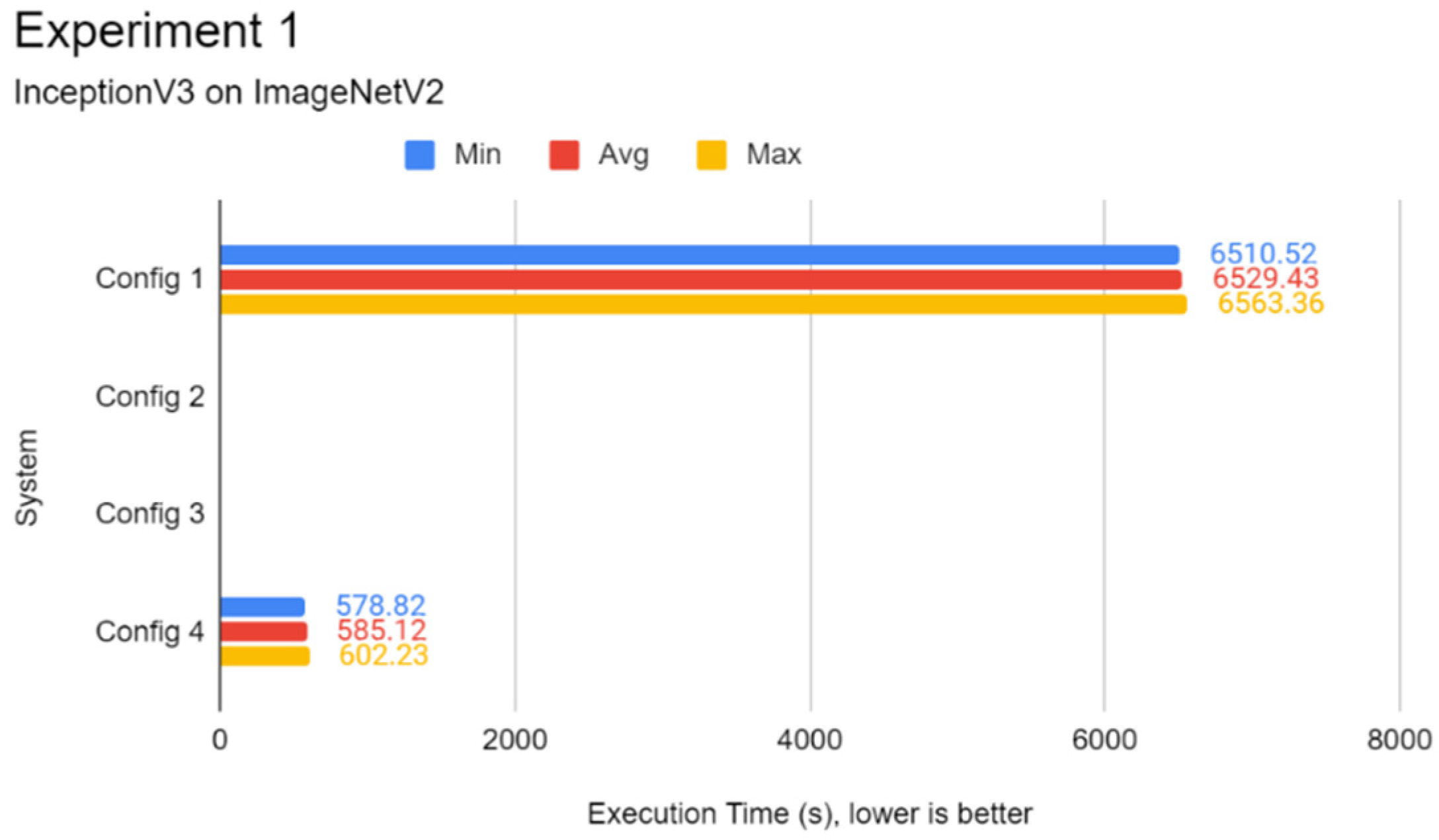
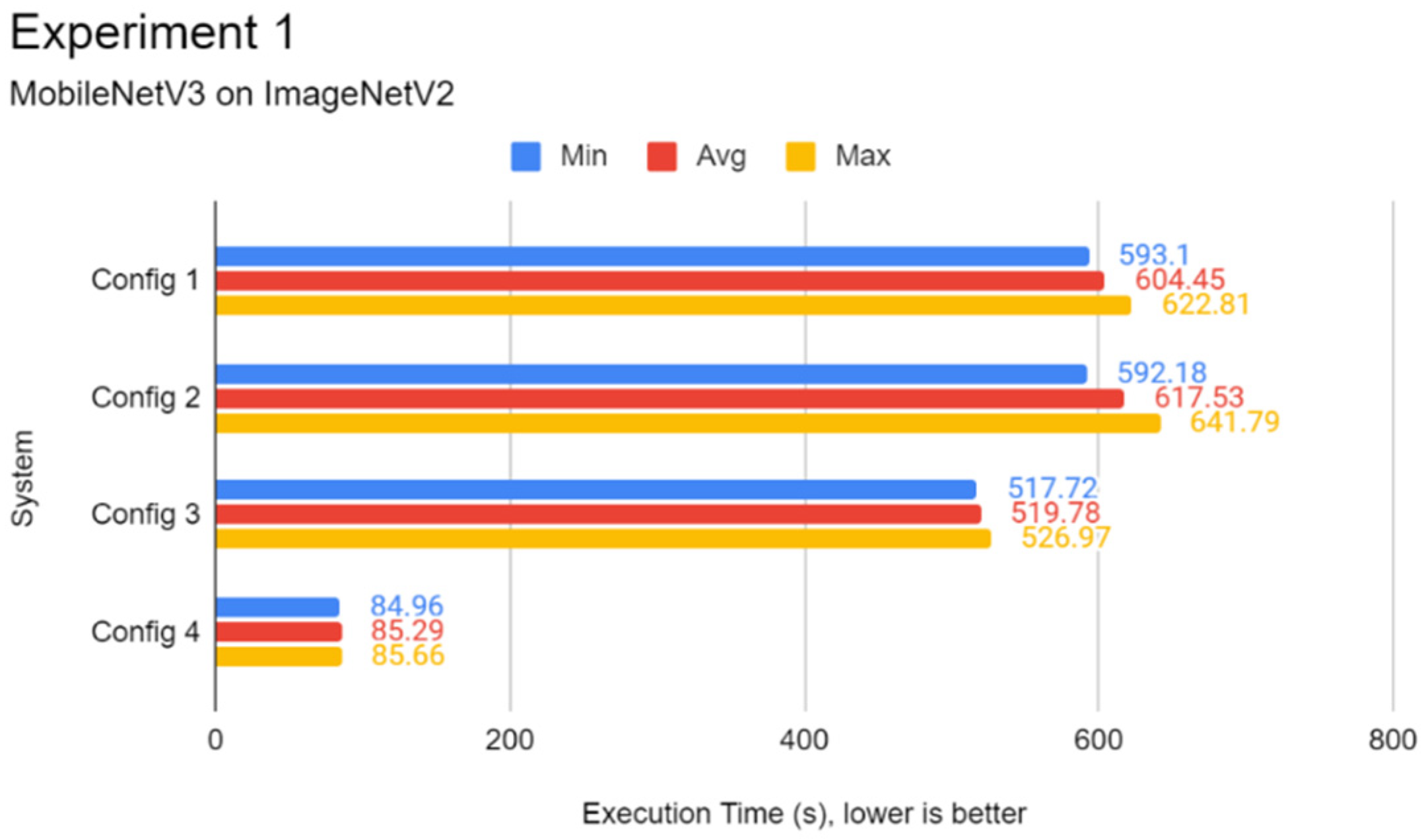
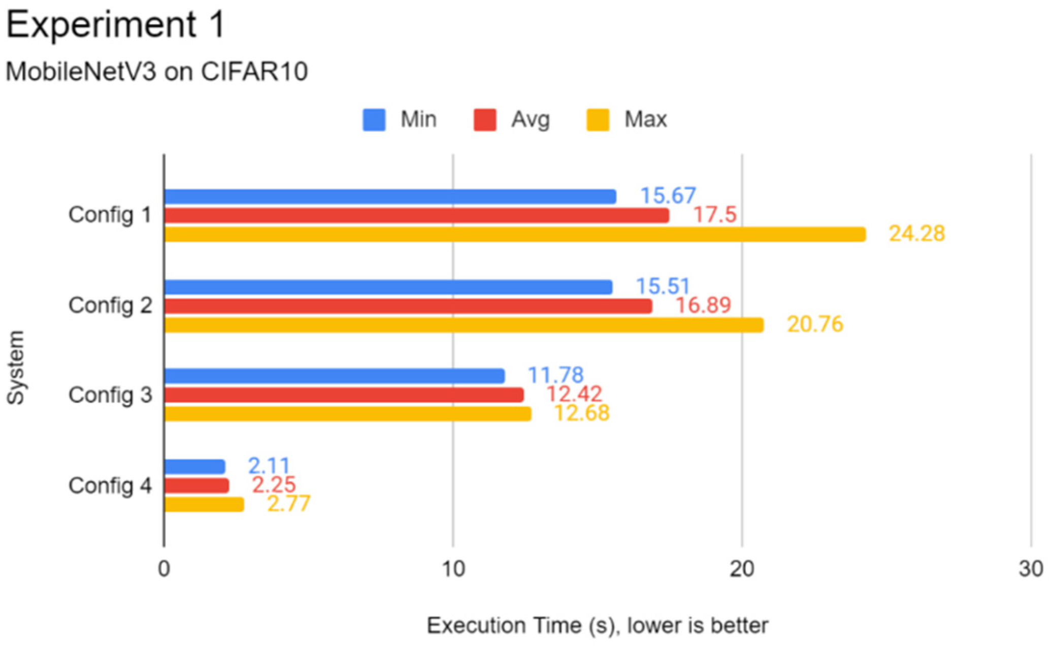
3.3. Experiment 1: Image Classification Inference Test

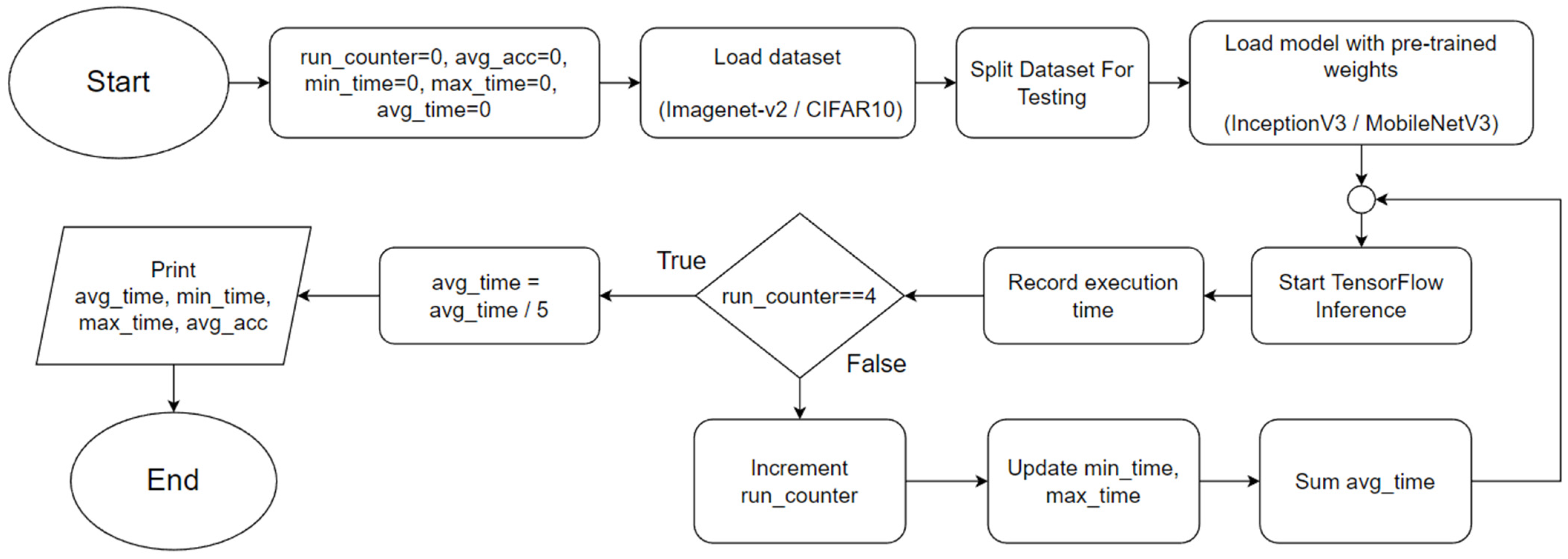
In this experiment, a comparison of the inference speed in classifying images from the ImageNetV2 test set and the test split of CIFAR10 was done across every system configuration on both pre-trained Inception-v3 and MobileNetV3 models. This experiment serves to evaluate the general image classification inference performance of all systems.

Since Python works best with 2 executors in Spark as per the findings in [12], and TensorFlow has official support only on Python, this experiment was carried out by running programs coded in Python. Each different program resulted in TensorFlow importing a different testing dataset, ImageNetV2 or CIFAR10, and the same applied to the loading of a pre-trained model, Inception-v3 or MobileNetV3. By running either program, TensorFlow would evaluate the model on the dataset and output its accuracy and the time taken for executing inference on the entire test dataset (the execution time), of which both were recorded at the end of each run. Each configuration was automatically run 5 times to produce consistent results and to reduce the likelihood of outliers. Minimum, maximum, and average values for execution time were recorded over 5 runs and then averaged into a single result. The flowchart for the Python program used in Experiment 1 is shown in Figure 1. Distributed versions of the programs are also included for use by the cluster systems.

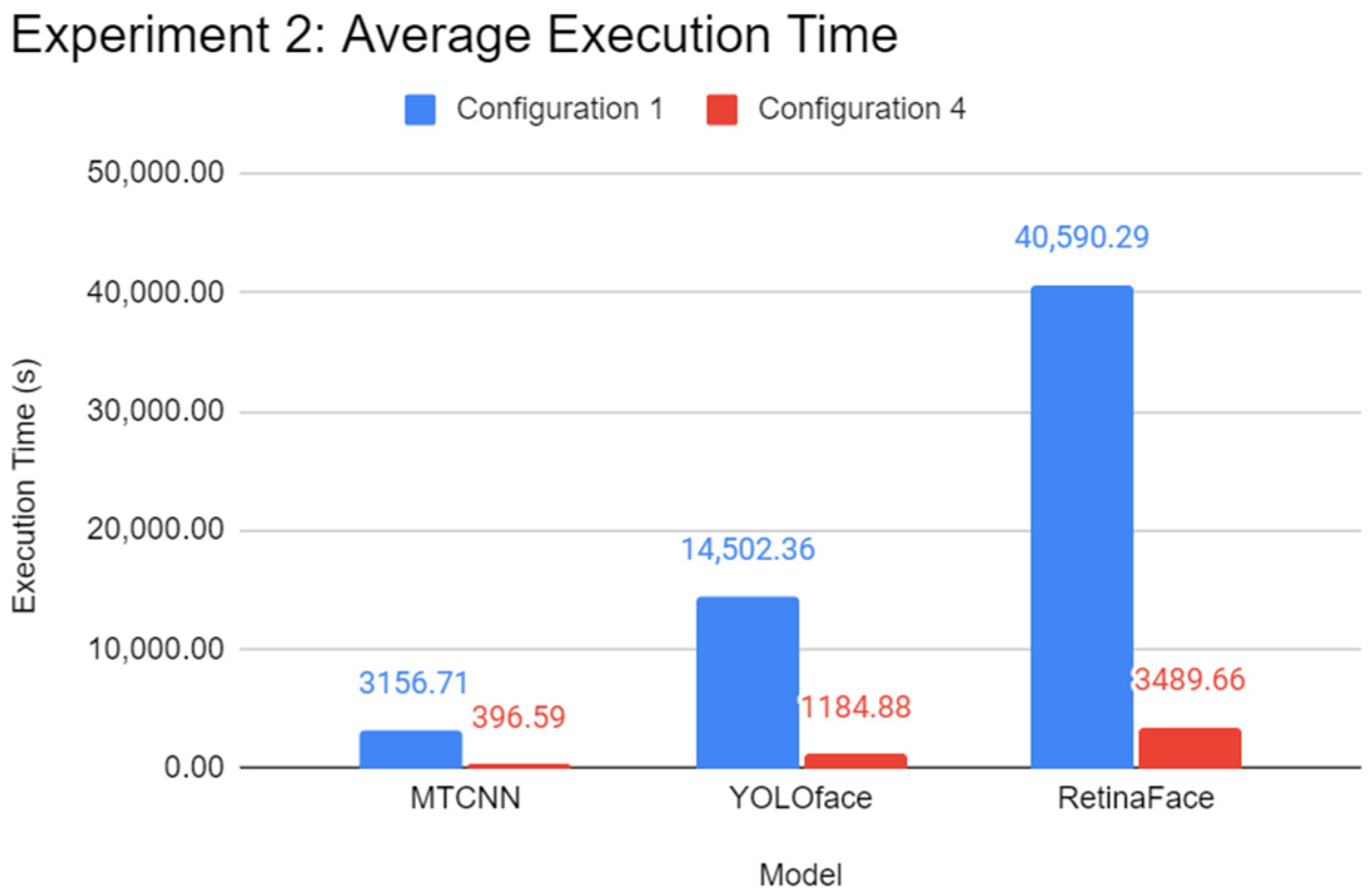
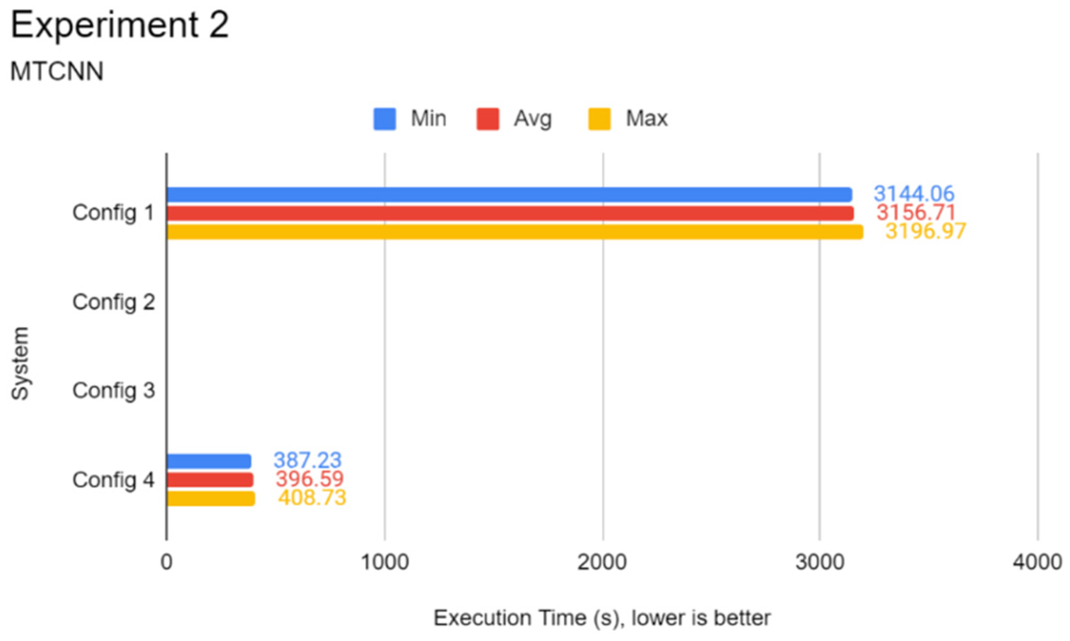
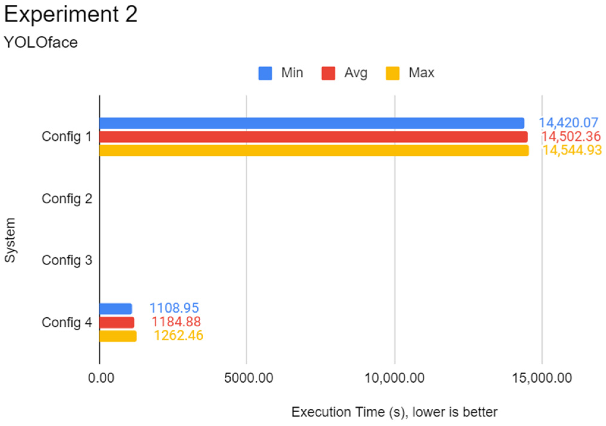
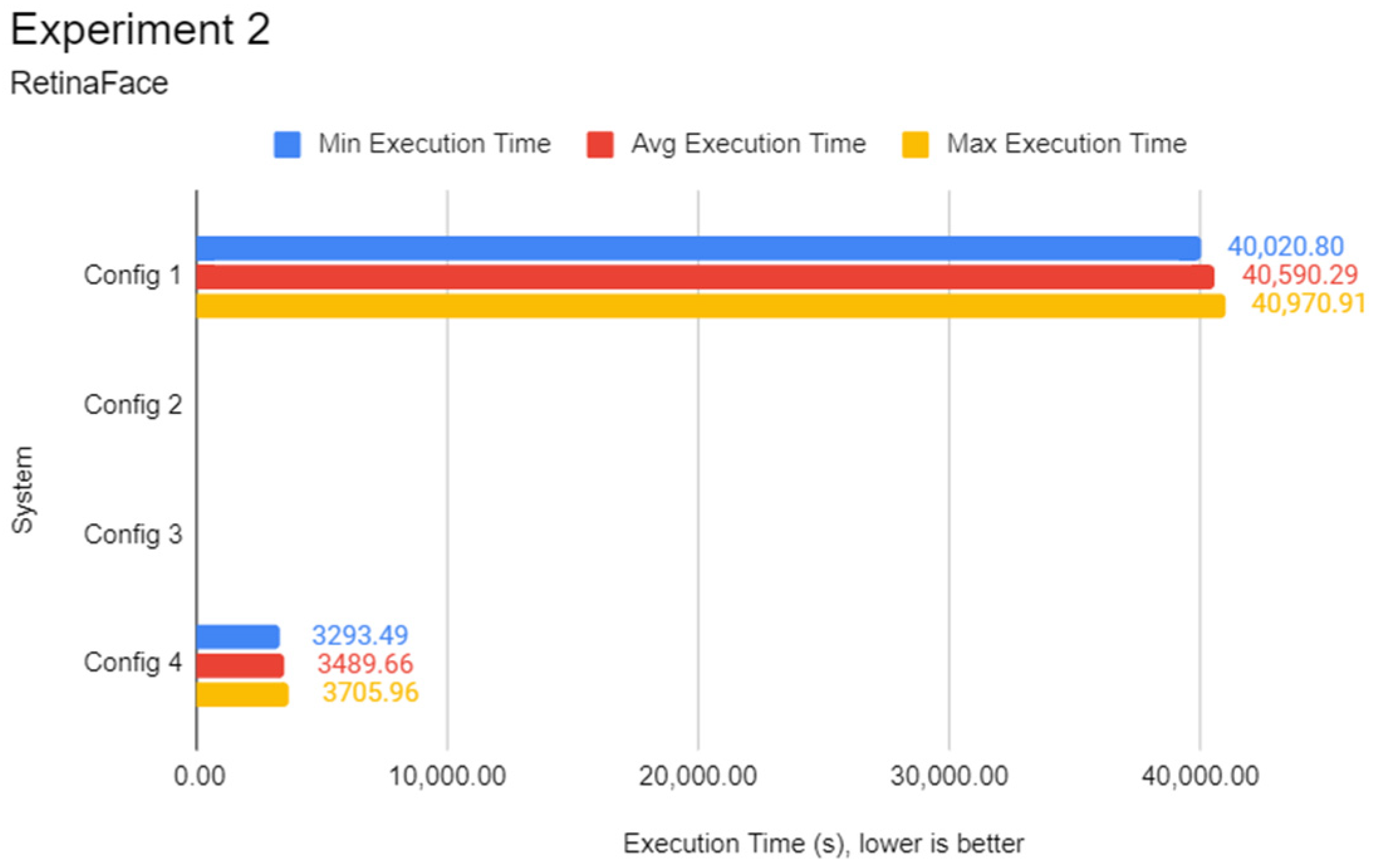
3.4. Experiment 2: Face Detection Test

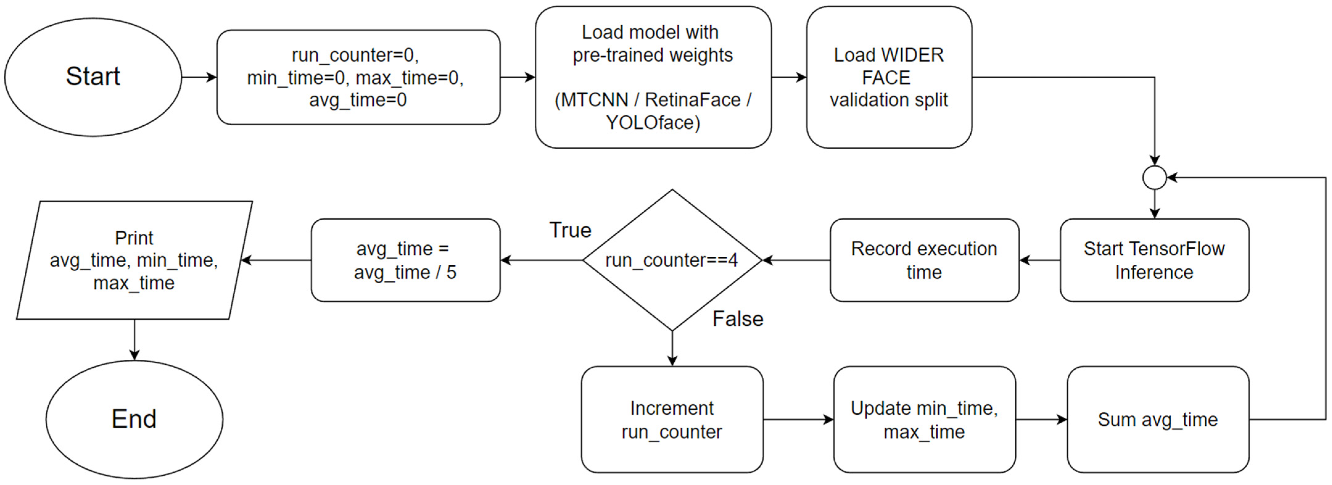
This experiment focuses on evaluating the inference performance of every system in face detection on a fixed dataset. Unlike the first experiment, CNN architectures such as Inception-v3 and MobileNetV3 are not used as they are architected with image classification tasks in mind. Instead, CNN architectures specialised in face detection such as RetinaFace, YOLOface, and MTCNN are used in this experiment on the WIDER FACE image dataset.

The procedures are identical to Experiment 1, except that Python programs coded specifically for this experiment initialise only the WIDER FACE validation dataset split. One of three Python programs contains a different face detection model, which can be RetinaFace, YOLOface, or MTCNN. Like Experiment 1, each Python program would be automatically run five times, the results recorded, and the next program with undocumented results chosen for subsequent testing until the results for every program were tested, respectively. RetinaFace was chosen as it is currently one of the most accurate face detection models available. YOLOface is essentially YOLOv3 trained on the WIDER FACE training dataset. MTCNN is a well-known face detection model with high detection accuracy and was chosen as the model benchmark for this experiment. Likewise, execution time was used as the sole primary metric for this experiment. Figure 2 shows the flowchart for the program used in Experiment 2.

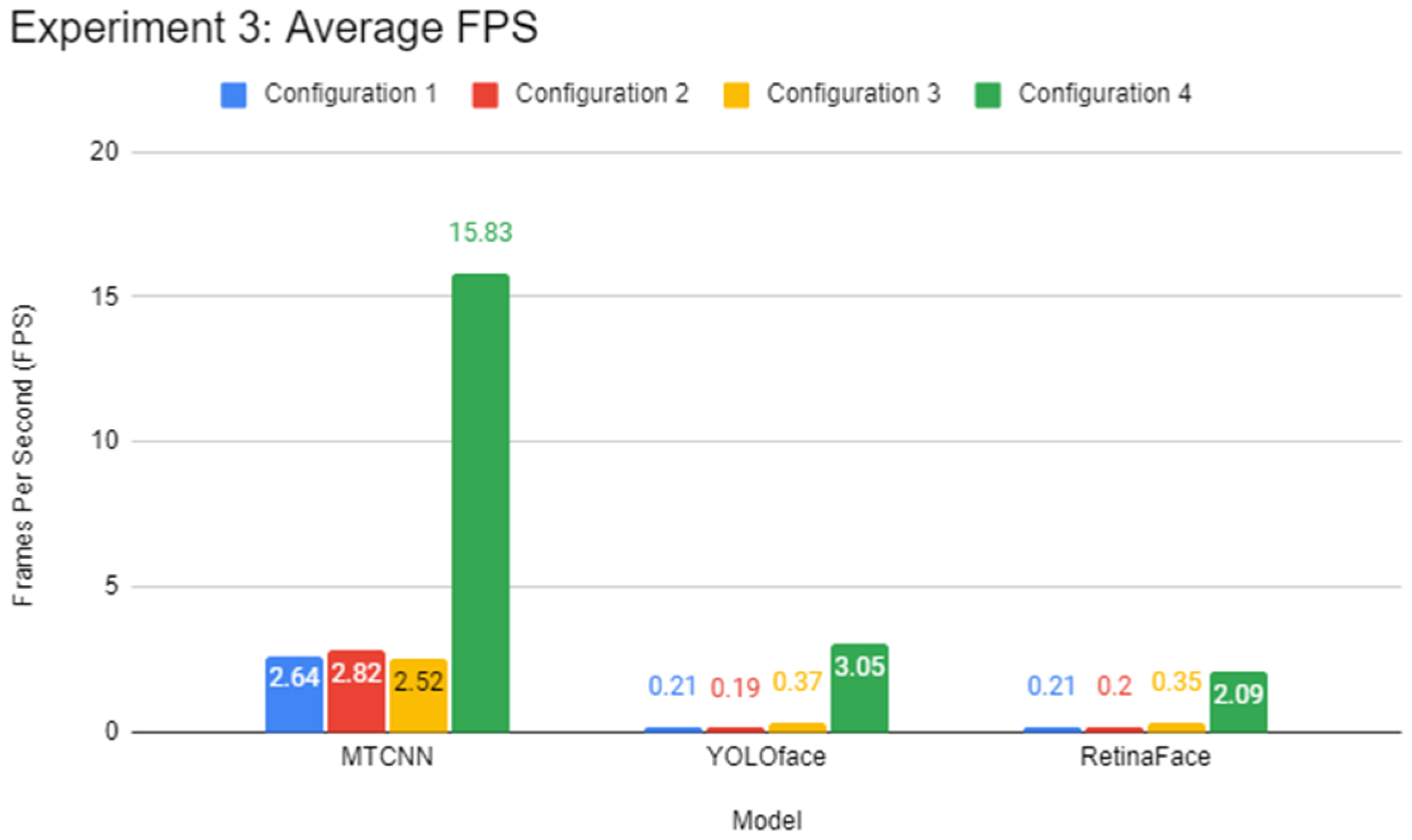
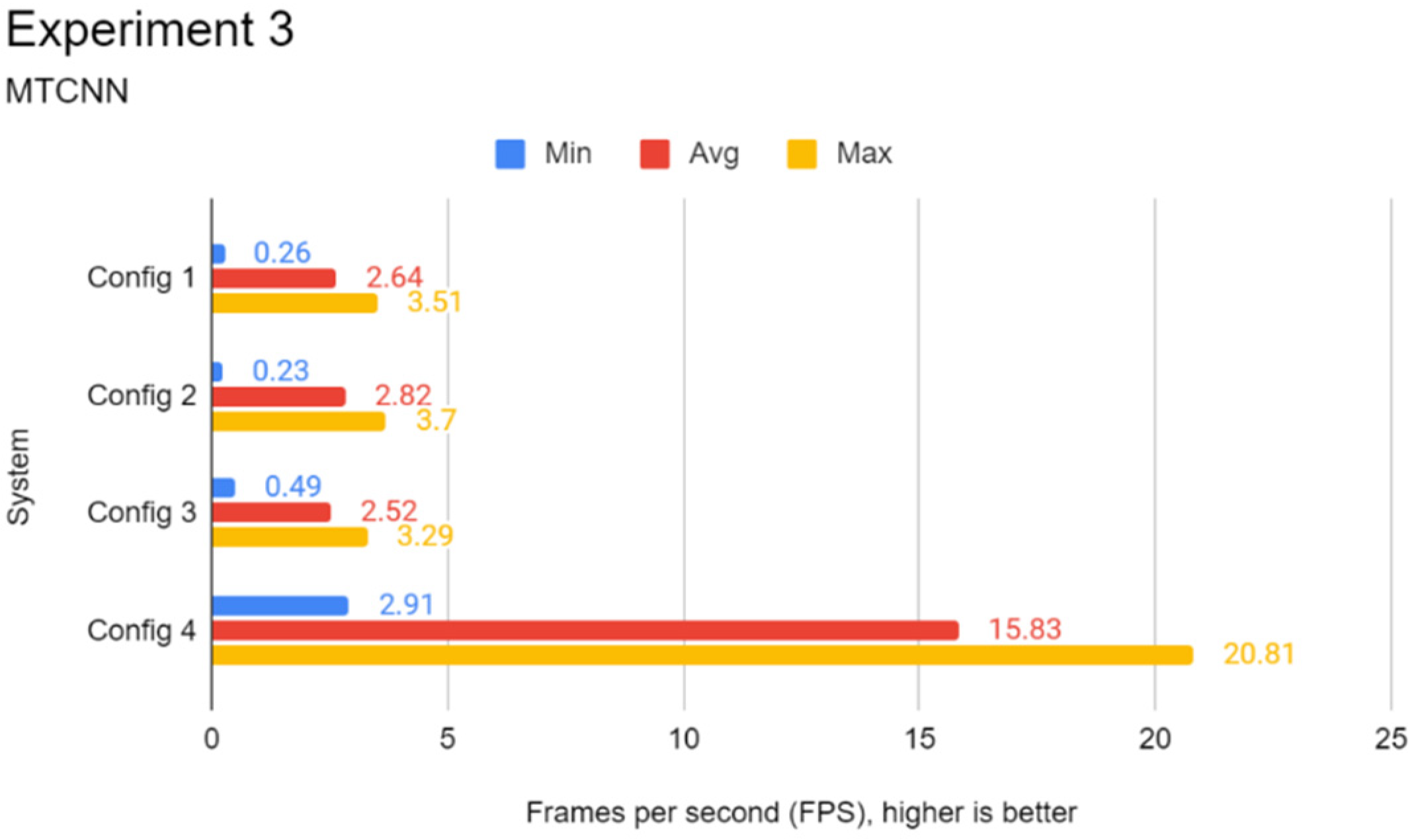
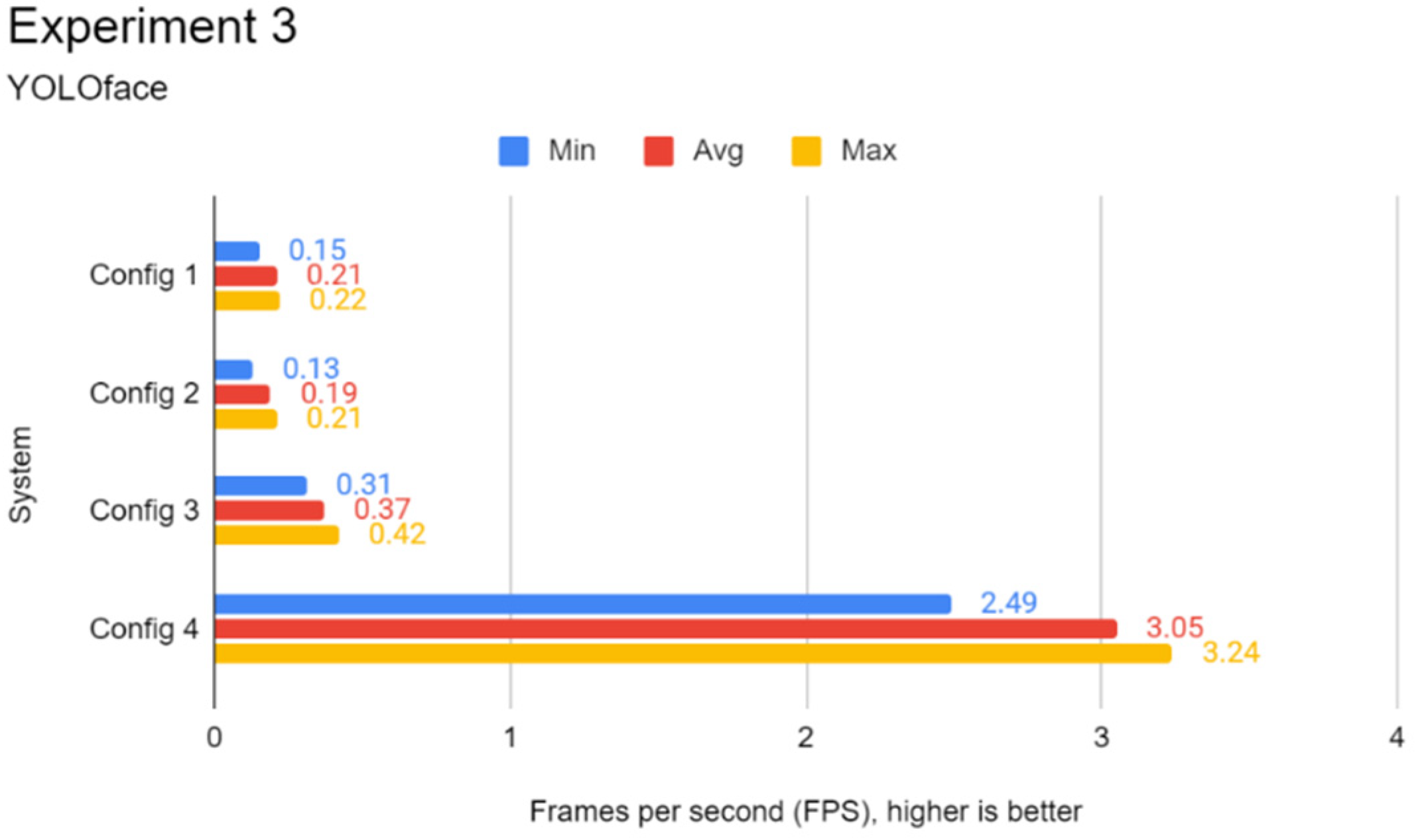
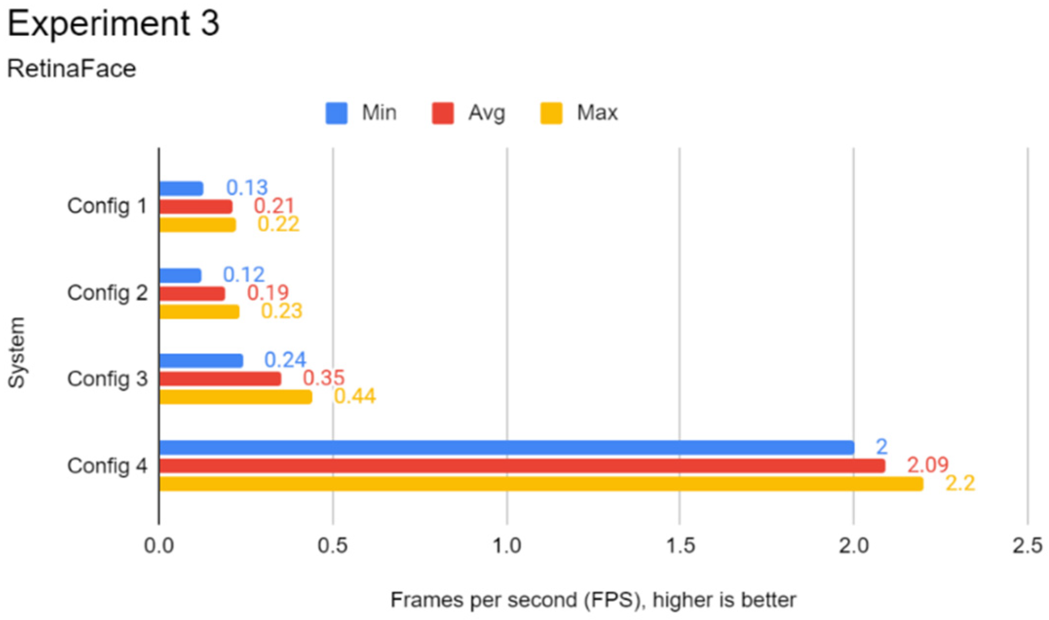
3.5. Experiment 3: Real-Time Face Detection Test

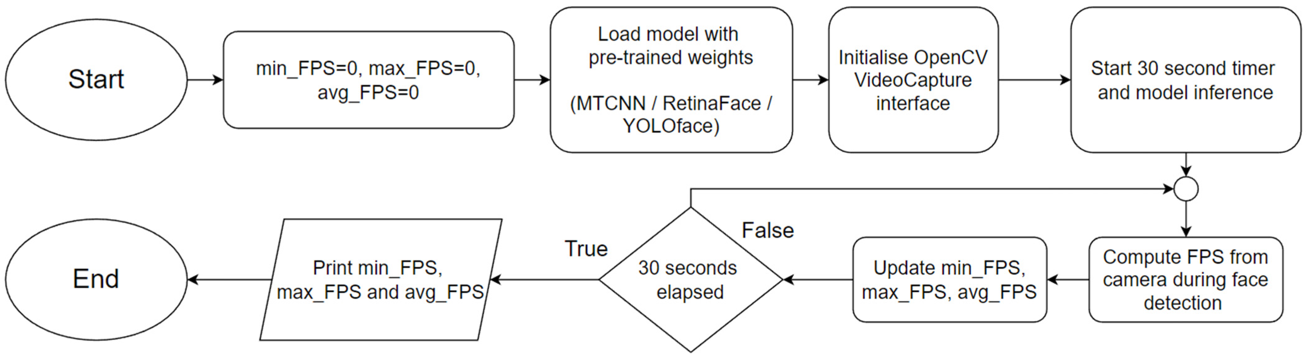
This experiment focuses on evaluating the performance of every configuration in face detection in real-time. Similar to Experiment 2, RetinaFace, YOLOface, and MTCNN were used as the face detection models for this experiment. The additional processing workload from rendering the frames from a video source poses a challenge to systems with weak processing hardware such as the Pi. As most recognition systems capture frames and process them in real-time, this experiment provides a good simulation of deploying the Pi in a production environment.

This experiment involved the use of the Redmi Note 5 Pro smartphone as a USB camera for real-time face detection. To clarify, frames were captured from the USB camera in real-time via OpenCV instead of using a dataset. Inference via a face detection model was then carried out on the captured frames via TensorFlow. Like Experiment 2, multiple Python programs were coded specifically for this experiment, utilising different face detection models to process the captured frames from the videos from OpenCV. When one of the chosen programs was launched, OpenCV would capture frames from the USB camera video footage continuously and the chosen model would carry out the inference on each of these video frames using either of the three face detection models. This experiment focused on camera FPS, which is retrieved directly from OpenCV. As the processing part of the face detection is performed on the systems and not on the phone camera itself, it is a good way to gauge the real-world performance of the systems if the face detection models are applied for production.

For this experiment, the procedure differed from the previous two experiments. Before the experiment began, the lead author was positioned in front of the USB camera, capturing the lead author from shoulders up. First, the procedure for this experiment involved launching one of the said programs. The lead author’s face would move side-to-side for 30 s. At the end of each run, the average FPS was recorded. Figure 3 shows the flowchart for Experiment 3.

3.6. Environment Configuration

This section explains the environmental configuration of all hardware and virtualized systems, as well as their respective system configurations used for the experiments. The hardware used in the experiments consisted of two Pi 4 Model B SBCs, a desktop computer with a dedicated GPU, and a Redmi Note 5 Pro smartphone for the USB camera. Two Pi 4 Model B SBCs that were similar in specifications were included in the experiment to evaluate the SBC’s performance in both standalone and clustered configurations. This was done in consideration of the findings in [12,16], which have shown diminishing performance returns with higher node counts. Thus, two nodes should eliminate any factor of diminishing performance gains, and it allows for evaluating the effectiveness of distributed inference. Four-gigabyte variants of the Pi 4 SBC were used for this experiment, and both used identical Class 10 microSD cards for storage. Like previous researchers, Raspberry Pi OS was used (formerly Raspbian) for these SBCs, as it is optimized for them. The lead author’s desktop computer was included in the experiment for virtualizing two low-end x86 virtual machines (VMs) as well as to act as a reference for the performance of other configurations. This system has 32 GB of DDR4 memory to cope with the worst memory-intensive operations possible such as running multiple VMs. Storage for the VMs and for the main machine was provided by a 256 GB Corsair MP510 solid-state drive (SSD). Windows 10 runs on the host system.

The Redmi Note 5 Pro was used to provide the USB webcam input via the Droidcam app on Android. The Redmi Note 5 Pro is connected to every system configuration used in the experiment through the v4l2loopback module in Linux, creating virtual cameras in the system configurations used. Based on the hardware used for the experiment, 4 configurations were set up as summarized in

Table 4. Systems used in the Experiments.

System	CPU	Memory (RAM)	Storage	Operating System
Configuration 1 (Pi 4B)	Quad-core ARM Cortex-A72 @ 1.5 GHz	4 GB LPDDR4	SanDisk 32 GB Class 10 microSD card	Raspberry Pi OS 10 64-bit
Configuration 2 (2-node Pi 4B cluster)	2 × (Quad-core ARM Cortex-A72 @ 1.5 GHz)	2 × (4 GB LPDDR4)	SanDisk 32 GB Class 10 microSD card	Raspberry Pi OS 10 64-bit
Configuration 3 (2-node VM cluster)	2 × (2 virtual Ryzen 5 3500X cores)	2 × (4 GB DDR4)	50 GB Virtual hard disk	Ubuntu 20.04 LTS
Configuration 4 (Desktop PC)	AMD Ryzen 5 3500X	32 GB DDR4	Corsair MP510 (256 GB)	Windows 10

.

3.7. Apache Spark: Standalone with HDFS, Cluster Setup & Job Execution

Spark is a data processing engine designed to replace or complement Hadoop’s MapReduce processing engine. The research experiments made use of the latest Spark version (3.2.1) for clustering multiple nodes and for single-node use. Configurations 2 and 3 ran Spark in standalone cluster deployment mode alongside the Hadoop Distributed File System (HDFS) which runs as a background service. As for Hadoop’s HDFS, the research experiments made use of Hadoop version 3.3.1. The replication factor for HDFS was set to the number of nodes, which in this case was 2.

Much like Hadoop and Spark-on-YARN, a Spark Standalone cluster has a master node in charge of coordinating and distributing all Spark jobs to all workers or working nodes of that cluster. To ease the entry of hostnames as worker nodes into the Spark environment file, the local IP addresses of the nodes for Configurations 2 and 3 were mapped to their respective hostnames in the /etc/hosts file, as these configurations use Linux operating systems, and this process was repeated in every node. As Spark requires Secure Shell (SSH) access, SSH fingerprints in the form of Rivest-Shamir-Adleman (RSA) keys were created on the master node. These keys were then placed in the worker nodes to verify and trust the master node. It is worth noting that a Spark node can be both a master and a worker at the same time. The hostnames of the nodes, which now map to their local IP addresses, were entered into the ‘workers’ file located under the Spark configuration folder. For checking whether all nodes were configured properly for Spark cluster use, the web UI for Spark was accessed via ‘(hostname): 8080’ in a web browser which displays the status of all nodes, including the master node.

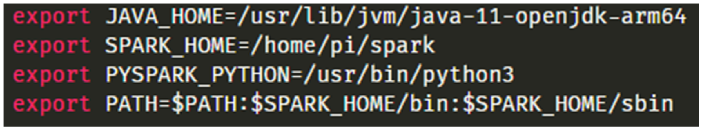
For all cluster systems, the following environment variables were set in the .bashrc file, as seen in Figure 4. These environment variables were required by Spark. As Spark is built on Java, using a compatible Java Development Kit (JDK) version was required. During initial testing, newer versions of JDK such as 14 and 17 failed to work, and thus the decision to revert to JDK 11 was made as it is the longest supported stable JDK version compatible with Spark at the time of writing. Since Configuration 2 runs on ARM architecture, an ARM64 version of the JDK developed by the open-source community (OpenJDK) was used in place of the traditional AMD64 architecture found in modern computers, which was also used for Configuration 3. The Spark folder containing all important binaries and configuration files was in the home directory of the user account for each cluster system. For Spark to use Python, ‘PYSPARK_PYTHON’ would have used the system’s default Python version, which was kept exactly at 3.8.10 across every node to prevent compatibility issues. The ‘SPARK_WORKER_CORES’ was set to the maximum number of cores available for a worker node, which in this case is 4 for Configuration 2 and ‘2’ for Configuration 3, as the Pi 4B is powered by a quad-core Broadcom SoC. Configuration 3 uses two cores from the host system for virtualization. ‘SPARK_WORKER_MEMORY’ was set to the total memory of the node minus 1 GB, which was 3 GB for both cluster systems to offer the best clustering performance and stability. Although ‘JAVA_HOME’ was already set in the .bashrc file, Spark mandated the JAVA_HOME environment variable in the Spark environment file, as it would refuse to launch without it declared and set. The value of the ‘SPARK_MASTER_HOST’ parameter varies for Configurations 2 and 3, as it was set to the local IP address of the master node for each of the Configurations.

For launching cluster-optimized versions of the programs used for the experiments, the spark-submit command was used to execute a SparkContext-containing Python program for the experiments, which was suited for experimenting.

3.8. Enhancement Methodology for Pi 4B

This section outlines a combination of enhancements that have a significant speedup impact on the Pi to further evaluate the effectiveness of these combined enhancements in contrast to a stock Pi. The enhancements consist of using the SSD, overclocking, and disabling the graphical user interface of the Pi. Initially, the use of neural accelerators such as the Intel Neural Compute Stick was considered. However, due to budget constraints, it was not possible to obtain such devices for testing their effectiveness. The authors highly recommend the use of neural accelerators for the Pi 4B to improve its DL performance where available.

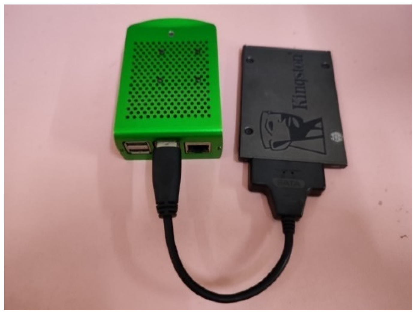
The Pi 4B has two hi-speed USB 2.0 ports and 2 super-speed USB 3.0 ports which allow the use of external storage solutions such as an external hard drive, flash drive, or even an SSD. The enhancement trials the use of SSD instead of the traditional Class 10 microSD card storage, which has inferior read and write speeds compared to the SSD. The SSD used in this test was a 120 GB Kingston A400 running off a 2.5-inch SATA-to-USB cable, as per Figure 5. The contents of the microSD card were cloned to the SSD using the ‘SD Card Copier’ program available in Raspberry Pi OS. During testing, it was found that using the USB 3.0 port for the SSD draws a significant amount of power from the Pi 4B, preventing the use of other peripherals such as the wireless network interface chip. Thus, the decision was made to stick to USB 2.0 for operability.

Typically, increasing the clock speed of the processor allows for more processing operations to be done in a second. This act of increasing clock speeds beyond designated specifications is called overclocking. To date, this has been the most effective method in increasing the processing performance of a system on all devices such as computers and smartphones. However, not every device allows overclocking access as it might void the warranty of a device. Overclocking on the Pi is achieved by setting a frequency beyond 1500 MHz in the config.txt file in the boot directory of the Raspberry Pi OS, which is the stock maximum permissible frequency of the Pi. For this paper, the clock speed was set to 1800 MHz with an overvoltage setting of 6 to help with stability. It was impossible to attempt a higher clock speed as the system failed to stabilise long enough for all tests to be complete.

By default, the Raspberry Pi OS includes a graphical user interface (or termed ‘desktop environment’ in the Linux community) based on the Lightweight X Desktop Environment (LXDE). However, there is still a motivation to know whether the standalone Pi will perform considerably better without the additional workload imposed by the rendering of LXDE, as the computing resource on the Pi is scarce. The ‘sudo systemctl set-default multi-user.target’ command was used to prevent the display server from being launched. This prevents the loading of graphical elements onto the screen and by extension, LXDE will not be loaded. The command forces the system to use a command-line interface.

4. Experiment Results

4.1. Performance Evaluation of Pi Spark Cluster

This section aims to provide a performance evaluation of the Pi 4B and an assessment of the effectiveness of distributed DL inference by using a Spark cluster of two Pi 4Bs by comparing its performance against a single Pi 4B in experiments. The three experiments that will be visited are concerned with investigating the feasibility of the Pi Spark cluster and providing a performance review of the latest generation of Pi 4B. Complete results, including minimum, average, and maximum values of the three experiments, can be found in Appendix A.

When testing InceptionV3 on either CIFAR10 or ImageNetV2, all cluster configurations utilising Spark failed to finish the test programs as per Figure 6. The systems crashed halfway during the experiment due to out-of-memory errors despite multiple retries. However, Configurations 1 and 4, which are standalone systems—the former being a single Pi 4B and the latter being the desktop PC—completed the test for 5 runs. Configuration 1, which took nearly 2 h to complete inference (6529.43 s), trailed Configuration 4 (585.12 s) by over 11 times to finish execution of an inference run using InceptionV3 on ImageNetV2. However, it is unsurprising given the hardware performance gap between the two configurations. Similarly, for CIFAR10, Configuration 1 took 3810.57 s, whereas Configuration 4 took 204.91 s, which is a difference of 18.6 times.

Referring to Figure 7, with using the MobileNetV3 model, all cluster configurations were able to finish normally. The difference between Configuration 2 and Configuration 1 is very negligible. The cluster was performing worse by 2% when running MobileNetV3 on ImageNetV2 on average. When the cluster was tested on CIFAR10, however, there seemed to be a 22% improvement in execution time, with a reduction of 3.78 s. Overall, the difference between using a cluster as opposed to the single Pi was not significant. Other than the results of the cluster systems, Configuration 4 eclipsed all system configurations by performing over 6 times faster than the Pi 4B in ImageNetV2, and around 7.7 times faster in CIFAR10. Configuration 1 held its ground and achieved respectable results in tests utilising MobileNetV3, as it achieved a speedup of 10.8 times in ImageNetV2 and 217.75 times in CIFAR10 against InceptionV3.

For Experiment 2 as per Figure 8, all cluster systems failed to finish all tests yet again by exhibiting the same behaviours seen in Experiment 1. Experiment 2 focused on just two configurations–Configurations 1 and 4. When testing with MTCNN on the WIDER FACE validation test set, Configuration 1 achieved an execution time of 3156.71 s on an average of 5 inference runs. Unsurprisingly, Configuration 4 achieved an average execution time of 396.59 s, which is close to 8 times faster than Configuration 1. When testing with YOLOface, the execution time for Configuration 1 jumped to 14,502.36 s on average, which is around 4.6 times slower than with MTCNN. Likewise, Configuration 4 experienced similar surges in the average execution time of 1184.88 s. Of the three models, the most processing-heavy model in this experiment is RetinaFace. Configuration 1 took 40,590.29 s to finish an inference run on the WIDER FACE validation test set, which is over 12 times slower than that of MTCNN. Configuration 4 took 3489.66 s to complete inference using RetinaFace on average, which is around 8.8 times slower compared to the time required by MTCNN to complete inference.

Much to the surprise of the authors, Experiment 3 is the only experiment where cluster configurations run without issues of running out of memory. This is possibly because of the low running time required for this specific experiment, with only 30 s of real-time face detection time. As per Figure 9, when testing live face detection with MTCNN, Configuration 1 achieved an average FPS of 2.64, which is expected of a heavy model. Its cluster counterpart, Configuration 2, achieved 2.82 FPS on average, a 7% increase. However, even Configurations 1 and 2 could surpass Configuration 3, respectively, with an average FPS of 2.52. Unexpectedly, Configuration 4 had an average FPS of 15.83, which is almost 6 times as much as the average FPS of Configuration 1.

With heavier models, such as RetinaFace, used for inference, average FPS was expected to plummet. Using YOLOface on Configuration 1 resulted in a measly average FPS of 0.21. Configuration 2 performed slightly worse with an average FPS of 0.19, which brings the benefits of clustering into question and raises doubts. Configuration 3 achieved an average FPS of 0.37, while Configuration 4 achieved an average FPS of 3.05, which is around 14.5 times more frames than Configuration 1. Despite this apparent gap, all configurations were not optimal for use with YOLOface due to low FPS of less than 1. Cameras typically have an FPS of somewhere between 18 and 30. If the system cannot carry out model inference on the captured frames in time, it will cause low FPS. Low FPS contributes to a very jittery image recognition performance, which can affect the usefulness of the recognition system.

The same scenario is repeated with RetinaFace. Configuration 1 achieved an average FPS of 0.19. Configuration 2 did not fare well either, as it only achieved around 0.20 FPS on average with an extremely negligible increase in FPS. Configuration 3 achieved an average FPS of 0.35, while Configuration 4 achieved an average FPS of 2.09. From the results, the average FPS figures were too low to be acceptable for real-time face detection at high frame rates for the two models, even on the desktop PC.

4.2. Test Results with Enhancements for Pi 4B (Configuration 1)

In contrast to Section 4.1, this section evaluates the performance of the enhanced Pi 4B and assesses the feasibility of using a Spark cluster of two Pi 4B versus using enhancements. In Experiment 1, as per

Table 5. Results for Experiment 1 using the enhancements for Pi 4B.

Test	Execution Time (s)		Enhancement Speedup
	Stock	Enhanced
InceptionV3 on ImageNetV2	6529.43	5765.84	1.13
InceptionV3 on CIFAR10	3810.57	3289.85	1.16
MobileNetV3 on ImageNetV2	828.33	553.59	1.50
MobileNetV3 on CIFAR10	20.67	16.31	1.27

, the average execution time with InceptionV3 on ImageNetV2 was noticeably reduced from 6529.43 to 5765.84 s, a reduction of 13.2%. The average execution time for CIFAR10 decreased from 3810.57 s to 3289.85 s, again achieving a reduction of 15.8%. Major reductions in average execution time were achieved when testing MobileNetV3 on ImageNetV2, where the average execution time for ImageNetV2 decreased from 828.33 s to 553.59 s, resulting in a speedup of 49.6%. Likewise, the average time on CIFAR10 was reduced from 20.67 s to 16.31 s, achieving a speedup of 26.7%. As expected, this combination set of enhancements achieved the lowest average execution time in all tests against the stock Pi 4B (without the enhancements). With these enhancements, the average execution time reduction was between 13.2% to 49.6% for Experiment 1, which is quite significant.

For Experiment 2, as per

Table 6. Results for Experiment 2 using the enhancements for Pi 4B.

Test	Execution Time (s)		Enhancement Speedup
	Stock	Enhanced
MTCNN	3156.71	2882.82	1.10
YOLOface	14,502.36	12,768.22	1.14
RetinaFace	40,590.29	35,948.35	1.13

, the enhanced Pi 4B had an average execution time of 2882.82 s using MTCNN. The reduction in execution time down from 3156.71 s made up a 9.5% improvement. When tested using YOLOface, the average execution time was slashed to 12,768.22 s from 14,502.36 s, a 13.6% reduction. The same trend was observed when the RetinaFace model was tested, where there is a reduction in execution time by 12.9%—from 40,590.29 s to 35,948.35 s. Overall, the combination of enhancements seemed to improve the general processing performance of Pi 4B.

As per

Table 7. Results for Experiment 3 using the enhancements for Pi 4B.

Test	Frames per Second (FPS)		Enhancement Speedup
	Stock	Enhanced
MTCNN	2.64	2.99	1.13
YOLOface	0.21	0.25	1.19
RetinaFace	0.21	0.23	1.10

, applying the enhancement combination to real-time MTCNN face detection resulted in a very slight increase of average FPS from 2.64 to 2.99—which is still a 13.3% increase in FPS. Nevertheless, the increase in FPS did not significantly help with the smoothness of face detection. The enhancements had little impact on YOLOface and RetinaFace, as underwhelming results were seen in both models during face detection carried out in real-time. The average FPS values saw an extremely negligible increase from 0.21 FPS to 0.25 FPS for YOLOface, and from 0.21 FPS to 0.23 FPS for RetinaFace. There is an improvement in average FPS between 9.5% to 19.5%. Even with the enhancements, the FPS for face detection with all complex models used in this experiment failed to exceed 10, leading to a suboptimal face detection performance.

5. Discussion

5.1. Ineffectiveness of Distributed DL Inference Using Pi

Based on the results of Configurations 2 and 3 in all experiments, the use of Spark cluster systems for the image processing tasks tested in all three experiments was ineffective, if not limiting. This ineffectiveness was highlighted when the cluster systems failed to complete an inference run with InceptionV3 on both CIFAR10 and ImageNetV2 datasets. Worse, these systems also failed to finish Experiment 2 with all 3 models. Regardless of the architecture of the cluster (Pi or VM), both systems exhibited the same out-of-memory (OOM) crash behaviour when executing inference with non-lightweight models (InceptionV3, RetinaFace) or on larger datasets like WIDER FACE. There were no crashes when testing programs in Experiment 3. It is suspected that the memory size of these complex models and the dataset could be responsible for this behaviour, as the clusters did not immediately crash when beginning testing but only several minutes into testing. It was later confirmed when TensorFlow warned about the lack of free memory allocation via the Spark output log, which subsequently caused the crash minutes into the tests.

Aside from the OOM issues, the results did not show any noticeable speedup as seen in

Table 8. Comparison of average execution time and speedup between a single Pi 4B and a 2-node Pi 4B cluster for Experiment 1.

Experiment 1 Test	Average Execution Time (s)		Speedup
	Pi 4B (Baseline)	2-Node Pi 4B Spark Cluster
MobileNetV3 on CIFAR10	20.67	16.89	1.22
MobileNetV3 on ImageNetV2	828.33	835.79	0.99

and

Table 9. Comparison of average FPS and speedup between a single Pi 4B and a 2-node Pi 4B cluster for Experiment 3.

Experiment 3 Test	Average FPS		Speedup
	Pi 4B (Baseline)	2-Node Pi 4B Spark Cluster
MTCNN	2.64	2.82	1.22
YOLOface	0.21	0.19	0.90
RetinaFace	0.21	0.20	0.95

, which is far from the expected values from 1.40 up to 2.00, especially as only two nodes were used to minimise the effect of diminishing performance returns associated with higher node counts. As per Figure 7a in [12], which was previously cited in Section 2.2, the authors of [12] used a Pi 4B Spark cluster for Spark MLlib workloads. There was a major reduction in the test set inference time from nearly 500 s to somewhere slightly above 200 s when two executors (nodes) were used instead of just one, which represents a speedup of 2.33. The inference results in this paper showed speedup values of less than 1 at 0.99, 0.90, and 0.95, which show slower inference speeds than a single node in some tests, and the cluster could only attain a speedup of 1.22. The slight speedup and the worse performance than running a single Pi completely contradicted the speedup scalability that was initially expected. While all the Pi clustering papers previously cited in Section 2.2 demonstrated speedup scalability across many nodes, the use of Spark TensorFlow Distributor for distributed inference in this paper did not show such scalability. Upon further investigation, it was found that the two executors were running the inference tests on their own, which may also be partly responsible for the OOM issue explored earlier. For context, the experiments utilised distributed versions of TensorFlow through the Spark TensorFlow Distributor, which is a library for Spark to distribute TensorFlow jobs to all executors. While Spark TensorFlow Distributor advertises distributed training, there was no explicit mention of distributed inference. However, support for distributed inference is obliquely suggested as the codebase in Spark TensorFlow Distributor has functions that support such a feature. This finding highlights the ineffectiveness of distributed DL inference when using the Spark TensorFlow Distributor even when the diminishing speedup factor was eliminated for the experiments. It is hoped that this finding will bring awareness towards implementing distributed DL inference in TensorFlow, as it is currently not the preferred option for ML/DL clustering solution for inference.

The most likely hypothesis for this is the lack of capability for distributing a model across different nodes. In a distributed training scenario, the same neural network model with unmodified architecture would be copied over to worker nodes as model replicas. This process speeds up training by comparing different accuracy and loss values in an epoch across all nodes. The node with the best-performing values has its parameters passed to some parameter server and the training process enters a new epoch until several epochs have been reached. Finally, the parameter server holds the best set of parameters that allow it to maximise accuracy and minimise loss, as seen in [28]. A neural network model in TensorFlow could not be partially distributed across worker nodes for inference as there is no method of segregating and re-joining the model architecture, given that the neural network models run in a top-down manner where data is passed layer after layer. This input dependency between layers renders the distribution of a neural network model impossible. Distributed inference in Spark TensorFlow Distributor is limited to copying the replica models over worker nodes. Ultimately, this results in the lack of speedup in cluster systems when running model inference. Spark TensorFlow Distributor is less preferred than Spark MLlib for the time being, as it could not increase inference performance with scale. At the time of writing, no other DL frameworks with adequate clustering support for inference tasks are available.

5.2. Performance Gap of Systems

Focusing on the standalone Pi 4B (Configuration 1), it is unsurprising to see a huge performance gap between the Pi and the desktop (Configuration 4) in all experiments as per

Table 10. Mean speedup against Configuration 1 in all experiments.

Experiment Tested	Model	Mean Speedup Against Configuration 1
		Config 1	Config 2	Config 4
Experiment 1	InceptionV3	1.00	-	14.41
	MobileNetV3		1.29	7.42
Experiment 2	MTCNN		0.19	7.96
	YOLOface		-	12.24
	RetinaFace			10.54
Experiment 3	MTCNN		0.89	6.00
	YOLOface		1.76	14.52
	RetinaFace		1.67	9.95

. When InceptionV3 was used for Experiment 1, the desktop was 14.41 times faster on average compared to the standalone Pi. The optimistic target was for the Pi cluster to perform closely to or outperform its VM counterpart (Configuration 3) in all experiments. However, results for cluster systems are not available, as they failed to finish inference run using InceptionV3. By using lightweight neural network models, the performance difference between the desktop and the Pi was reduced to 7.42 times. This may suggest that the Pi could remain competitive with modern hardware when a model with lightweight architecture is used. The VM cluster is operating as a de facto single VM because of the phenomenon explained in Section 5.1. It was only 29% faster than the Pi, which also highlights the fact that the performance difference between the two systems may not be as drastic as initially expected. In Experiment 2, using a lightweight model also reflects the same trend, as the desktop was only 7.96 times faster than the Pi in MTCNN compared to a difference of 12.24 times in YOLOface and 10.54 times in RetinaFace, respectively. Once again, the results for cluster systems are absent due to the issues mentioned in the previous section. For Experiment 3, the standalone Pi outperformed the VM cluster by 11% in MTCNN. The desktop PC still outperformed the Pi by a difference of sixfold. When using both YOLOface and RetinaFace, the average difference between the Pi and desktop PCs widened to close to tenfold, where it was 14.52 times faster in YOLOface and 9.95 times faster in RetinaFace, respectively. The same case is reflected in the VM cluster, where it was 1.76 times faster in YOLOface and 1.67 times faster in RetinaFace, respectively.

Overall, the desktop PC still outperforms the Pi multiplicatively because of the hardware difference between the two systems. However, this discovery of the reduction in performance gap when using lightweight models for inference suggests that using lightweight neural network models for Pi is vital to maintaining competitiveness in most applications using DL against modern hardware. This is especially true when the performance difference between the desktop PC and the Pi was reduced when using lightweight DL models as opposed to standard DL models. While the Pi could barely keep up with the VM cluster, the performance difference between the VM cluster and the Pi was not drastic as initially expected. This shows that the Pi can rival the VM, which itself is a simulation of a low-end system created for this performance review.

Referring to

Table 11. Accuracy and speedup differences over InceptionV3 using MobileNetV3 for Configuration 1.

Experiment 1 Test		Execution Time (s)	Speedup Over InceptionV3	Accuracy Difference
Dataset	Model
CIFAR10	InceptionV3	3810.57	184.35	25%
	MobileNetV3	20.67
ImageNetV2	InceptionV3	6529.43	7.88	12%
	MobileNetV3	828.33

, using lightweight models for the Pi massively reduces execution time at the cost of accuracy. Execution time in ImageNetV2 was reduced from 6529.43 s to only 828.33 s. This helped in achieving a reduction in execution time by 7.88 times, while the accuracy was reduced only by 12%. In CIFAR10, the execution time was reduced from 3810.57 s to just 20.67 s, which is an overwhelming reduction of 184.35 times at the cost of a 25% decrease in accuracy. Regardless, the authors were surprised that the Pi could achieve close to 3 FPS using MTCNN for face detection, even though it was suboptimal for real-world usage.

Based on Figure 10, using the enhancements for the Pi helped to achieve noticeable speedups where the optimised Pi was 26% faster in Experiment 1, 12% faster in Experiment 2, and 14% faster in Experiment 3 on average against a Pi that has not undergone optimisation. When considering the mean speedup figures from all experiments, the optimised Pi was 17% faster on average. From the authors’ point of view, the optimised Pi was driven to the very limit of performance and all viable optimisation attempts were exhausted to achieve such speedup. For the time being, there are no other optimisation attempts available that do not require dependence on optimising the software code that the Pi runs on. This leads to the same outcome where more emphasis on the use of lightweight models is required to compensate for the lack of powerful processing hardware found in the Pi 4B. It still outperformed its 2-node Spark cluster counterpart.

5.3. The State of Distributed DL Inference Using Spark TensorFlow Distributor

To recap, this paper mainly researched the effectiveness of distributed DL inference by using a 2-node Pi cluster. Contrary to the expectations of the authors, adding another Pi node for DL inference offered no significant speedup as there was no significant performance difference between the 2-node Pi cluster and the single Pi. Occasionally, the cluster performed worse than its standalone counterpart in some parts of the experiments.

Using just two Pi 4B nodes for processing-heavy Spark programs in standalone mode is also not recommended, as there would be memory allocation issues, particularly with the executor and driver. As all the nodes only had 4 GB of RAM, this might have played a major role in this outcome. From this, the RAM capacity for a 2-node cluster configuration should have the appropriate amount of RAM depending on the use case of the application, as it is hard to find out the minimum amount of RAM capacity that will eliminate memory exceptions. For this reason, referring to the Apache Spark documentation is highly recommended, as every Spark application will have different resource requirements. For the experiments seen in this report, the minimum is ideally 6 GB, as DL models such as the InceptionV3 alone could easily occupy 3 GB of RAM during model inference. The size of the dataset is also a factor, as ImageNetV2 was found to have occupied 2 GB of RAM during testing. Another way to work around the memory limitations is to run Spark on YARN, though this is not ideal as it introduces processing overhead as per the discovery in [29]. In summary, it is better to use a single Pi which would be better off being enhanced as per the findings of this report.

At the time of writing, the technology behind the distributed version of TensorFlow, the Spark TensorFlow Distributor, has not matured enough to allow for distributed inference that scales well with the number of nodes in a cluster, as currently, each node is still executing inference independently without synchronisation across the cluster. The authors deliberate that the Spark MLlib library will remain the status quo of the go-to ML framework for use with Spark clusters.

6. Conclusions

In summary, the findings of this research paper have successfully addressed the need to investigate the use of the TensorFlow framework for Spark cluster systems, which to the authors’ knowledge is one of the earliest findings based on the suggestion of fellow researchers. The performance difference between a 2-node Pi 4B Spark cluster and a Pi 4B has been studied successfully. For the time being, it is currently not advised to use a Pi 4B cluster for distributed DL because of the state of immaturity in DL frameworks beyond SparkML like TensorFlow, as confirmed by the lack of performance scalability in inference tasks seen in the results. The authors believe these findings will motivate fellow researchers and the TensorFlow team to pursue a scalable distributed inference solution that will allow multiple low-end devices to perform in tandem, especially in an age where semiconductor shortage is rampant, and hopefully, such a solution shall eliminate the status quo of SparkML as the preferred distributed ML framework.

Through the experiments, the performance gap between a Pi and a standard mid-end system in inference tasks was also identified. The differences lie between 6 to 15 times, depending on the complexity of the DL model. It was found that using a lightweight DL model can help reduce the performance deficit between powerful systems and low-end embedded devices like the Pi 4B as opposed to complex models. Therefore, low-end embedded devices can carry out lightweight DL inference competitively with their more powerful counterparts. In the experiments of this report, the Pi 4B could keep up with the VM cluster in lightweight inference most of the time while falling behind on heavier tasks, which is possibly attributed to a hardware-level architecture difference. The use of state-of-the-art face detection models, which can achieve extremely high accuracies, requires an ample amount of processing power. The authors highly recommend lightweight, CPU-optimised neural network models for simple DL applications.

This paper has also optimised the Pi 4B, and results have shown that the enhancement helped the Pi perform 17% faster on average than its standalone and 2-node cluster counterparts, albeit with the addition of the SSD. However, the use of SSD may not have made a major impact on the image processing performance of the Pi. For those seeking to optimise the Pi, the switch to SSD is not mandatory for performance gains—in fact, it increases the price–performance proposition of the Pi. Until distributed inference solutions are available, the concept of distributed DL inference remains a theoretical concept for the time being, and optimising remains key to increasing the performance of the Pi. Undoubtedly, the computational power of a single Pi 4B would still suffice in lightweight ML and DL inference tasks, as seen through the results of the experiments.

The authors would like to remind the reader that the Pi is a general-purpose embedded device suitable for nearly every use case. Thus, the lack of neural acceleration is to be expected, as DL is not Pi’s major use case. For those opting for an embedded device for more complex DL inference tasks, the better price–performance option would be an AI-accelerated SBC such as the Nvidia Jetson Nano at $149, as it outperforms the Pi 4B by a huge margin as per the results in [13]. Alternatively, a neural accelerator such as an Intel Neural Computing Stick can also help boost the DL performance of the Pi, as seen in [14]. If an embedded system is not the primary focus and where permissible, a low-cost PC with AI acceleration via a single powerful discrete GPU is also recommended. If hardware solutions are not an option, lightweight ML/DL models in TensorFlow can readily be converted into the TensorFlow Lite versions to further improve inference speed. Progress on distributed inference for cluster systems needs to be made for the feasibility of low-end device clusters to come to fruition. Before that, the ideal cluster deployment mode for PySpark jobs must be implemented in place of the less-reliable client mode. Regarding the previous statement, the authors also suggest that the Apache Spark development team and the TensorFlow development team collaborate in addressing this specific scope of distributed systems, which may be niche by nature but will enable low-cost distributed DL inference that will suffice as a viable alternative to a single powerful system for such purposes.

Additional work on investigating the benefits of using the Spark TensorFlow Distributor is required, as model inference seems to be ineffective. Future work in this study would be to verify the performance benefits of distributed training of DL models using Spark TensorFlow Distributor. Instead of using a Pi cluster, a distributed system containing multiple GPUs would be used for this investigation. A performance comparison between Spark MLlib and Spark TensorFlow Distributor by training models of identical architecture should also be considered for investigating the use of DL frameworks outside the Spark ecosystem. Other DL frameworks, like PyTorch, could be trialled against TensorFlow in investigating the ideal scalable DL framework.

References

1. Shinde, P.P.; Shah, S. A review of machine learning and deep learning applications. In Proceedings of the 2018 Fourth International Conference on Computing Communication Control and Automation (ICCUBEA), Pune, India, 16–18 August 2018; pp. 1–6. [Google Scholar]
2. Razzak, M.I.; Naz, S.; Zaib, A. Deep learning for medical image processing: Overview, challenges and the future. In Classification in BioApps; Dey, N., Ashour, A.S., Borra, S., Eds.; Springer: Cham, Switzerland, 2018; pp. 323–350. [Google Scholar]
3. Hatt, M.; Parmar, C.; Qi, J.; El Naqa, I. Machine (deep) learning methods for image processing and radiomics. IEEE Trans. Radiat. Plasma Med. Sci. 2019, 3, 104–108. [Google Scholar] [CrossRef]
4. Abadi, M.; Barham, P.; Chen, J.; Chen, Z.; Davis, A.; Dean, J.; Zheng, X. TensorFlow: A System for Large-Scale Machine Learning. In Proceedings of the 12th USENIX Symposium on Operating Systems Design and Implementation (OSDI 16), Savannah, GA, USA, 2–4 November 2016; pp. 265–283. [Google Scholar]
5. Gupta, A.; Gandhi, C.; Katara, V.; Brar, S. Real-time video monitoring of vehicular traffic and adaptive signal change using Raspberry Pi. In Proceedings of the 2020 IEEE Students Conference on Engineering & Systems (SCES), Prayagraj, India, 10–12 July 2020; pp. 1–5. [Google Scholar]
6. Gupta, I.; Patil, V.; Kadam, C.; Dumbre, S. Face detection and recognition using Raspberry Pi. In Proceedings of the 2016 IEEE International WIE Conference on Electrical and Computer Engineering (WIECON-ECE), Pune, India, 19–21 December 2016; pp. 83–86. [Google Scholar]
7. Patel, K.; Patel, M. Smart Surveillance System using Deep Learning and RaspberryPi. In Proceedings of the 2021 8th International Conference on Smart Computing and Communications (ICSCC), Kochi, India, 1–3 July 2021; pp. 246–251. [Google Scholar]
8. Anh, P.T.; Duc, H.T.M. A Benchmark of Deep Learning Models for Multi-leaf Diseases for Edge Devices. In Proceedings of the 2021 International Conference on Advanced Technologies for Communications (ATC), Ho Chi Minh City, Vietnam, 14–16 October 2021; pp. 318–323. [Google Scholar]
9. Cloutier, M.; Paradis, C.; Weaver, V. A Raspberry Pi Cluster Instrumented for Fine-Grained Power Measurement. Electronics 2016, 5, 61. [Google Scholar] [CrossRef] [Green Version]
10. Hajji, W.; Tso, F. Understanding the Performance of Low Power Raspberry Pi Cloud for Big Data. Electronics 2016, 5, 29. [Google Scholar] [CrossRef]
11. Rahmat, R.F.; Saputra, T.; Hizriadi, A.; Lini, T.Z.; Nasution, M.K. Performance test of parallel image processing using open MPI on Raspberry PI cluster board. In Proceedings of the 2019 3rd International Conference on Electrical, Telecommunication and Computer Engineering (ELTICOM), Medan, Indonesia, 16–17 September 2019; pp. 32–35. [Google Scholar]
12. Komninos, A.; Simou, I.; Gkorgkolis, N.; Garofalakis, J.D. Performance of Raspberry Pi microclusters for Edge Machine Learning in Tourism. In Proceedings of the European Conference on Ambient Intelligence 2019, Rome, Italy, 13–15 November 2019; pp. 8–18. [Google Scholar]
13. Süzen, A.A.; Duman, B.; Şen, B. Benchmark analysis of jetson tx2, jetson nano and raspberry pi using deep-cnn. In Proceedings of the 2020 International Congress on Human-Computer Interaction, Optimization and Robotic Applications (HORA), Ankara, Turkey, 26–28 June 2020; pp. 1–5. [Google Scholar]
14. Yoshimoto, J.; Taniguchi, I.; Tomiyama, H.; Onoye, T. An Evaluation of Edge Computing Platform for Reliable Automated Drones. In Proceedings of the 2020 International SoC Design Conference (ISOCC), Yeosu, Korea, 21–24 October 2020; pp. 95–96. [Google Scholar]
15. Papakyriakou, D.; Kottou, D.; Kostouros, I. Benchmarking Raspberry Pi 2 Beowulf Cluster. Int. J. Comput. Appl. 2018, 179, 21–27. [Google Scholar] [CrossRef]
16. Srinivasan, K.; Chang, C.Y.; Huang, C.H.; Chang, M.H.; Sharma, A.; Ankur, A. An efficient implementation of mobile raspberry Pi hadoop clusters for robust and augmented computing performance. J. Inf. Process. Syst. 2018, 14, 989–1009. [Google Scholar]
17. Samadi, Y.; Zbakh, M.; Tadonki, C. Comparative study between Hadoop and Spark based on Hibench benchmarks. In Proceedings of the 2016 2nd International Conference on Cloud Computing Technologies and Applications (CloudTech), Marrakech, Morocco, 24–26 May 2016; pp. 267–275. [Google Scholar]
18. Biørn-Hansen, A.; Grønli, T.M.; Ghinea GAlouneh, S. An empirical study of cross-platform mobile development in industry. Wirel. Commun. Mob. Comput. 2019, 2, 1–12. [Google Scholar] [CrossRef]
19. Mantowsky, S.; Heuer, F.; Bukhari, S.; Keckeisen, M.; Schneider, G. ProAI: An Efficient Embedded AI Hardware for Automotive Applications-A Benchmark Study. In Proceedings of the IEEE/CVF International Conference on Computer Vision, Montreal, QC, Canada, 11–17 October 2021; pp. 972–978. [Google Scholar]
20. Bordin, M.V. A Benchmark Suite for Distributed Stream Processing Systems. Master’s Thesis, Federal University of Rio Grande do Sul, Rio Grande do Sul, Brazil, May 2017. [Google Scholar]
21. Recht, B.; Roelofs, R.; Schmidt, L.; Shankar, V. Do imagenet classifiers generalize to imagenet? In Proceedings of the 36th International Conference on Machine Learning, Long Beach, CA, USA, 9–15 June 2019; pp. 5389–5400. [Google Scholar]
22. Krizhevsky, A.; Hinton, G. Learning Multiple Layers of Features from Tiny Images; Technical Report TR-2009; University of Toronto: Toronto, ON, Canada, 2009. [Google Scholar]
23. Yang, S.; Luo, P.; Loy, C.C.; Tang, X. Wider face: A face detection benchmark. In Proceedings of the IEEE Conference on Computer Vision and Pattern Recognition, Las Vegas, NV, USA, 27–30 June 2016; pp. 5525–5533. [Google Scholar]
24. Zhang, K.; Zhang, Z.; Li, Z.; Qiao, Y. Joint face detection and alignment using multitask cascaded convolutional networks. IEEE Signal Process. Lett. 2016, 23, 1499–1503. [Google Scholar] [CrossRef] [Green Version]
25. Deng, J.; Guo, J.; Ververas, E.; Kotsia, I.; Zafeiriou, S. Retinaface: Single-shot multi-level face localisation in the wild. In Proceedings of the IEEE/CVF Conference on Computer Vision and Pattern Recognition, Seattle, WA, USA, 13–19 June 2020; pp. 5203–5212. [Google Scholar]
26. Chun, L.Z.; Dian, L.; Zhi, J.Y.; Jing, W.; Zhang, C. YOLOv3: Face detection in complex environments. Int. J. Comput. Intell. Syst. 2022, 13, 1153–1160. [Google Scholar] [CrossRef]
27. Xiang, J.; Zhu, G. Joint face detection and facial expression recognition with MTCNN. In Proceedings of the 2017 4th international conference on information science and control engineering (ICISCE), Changsha, China, 21–23 July 2017; pp. 424–427. [Google Scholar]
28. Li, M.; Andersen, D.G.; Park, J.W.; Smola, A.J.; Ahmed, A.; Josifovski, V.; Long, J.; Shekita, E.J.; Su, B.Y. Scaling distributed machine learning with the parameter server. In Proceedings of the 11th USENIX Symposium on Operating Systems Design and Implementation (OSDI 14), Broomfield, CO, USA, 6–8 October 2014; pp. 583–598. [Google Scholar]
29. Mavridis, I.; Karatza, H. Performance evaluation of cloud-based log file analysis with Apache Hadoop and Apache Spark. J. Syst. Softw. 2017, 125, 133–151. [Google Scholar] [CrossRef]
Figure 1. General flowchart for the Python programs used in Experiment 1.
Futureinternet 14 00220 g001
Figure 2. General flowchart for the Python programs used in Experiment 2.
Futureinternet 14 00220 g002
Figure 3. General flowchart for the Python programs used in Experiment 3.
Futureinternet 14 00220 g003
Figure 4. Environment Variables for 2-node Pi Cluster.
Futureinternet 14 00220 g004
Figure 5. External SSD connected to a Pi 4B.
Futureinternet 14 00220 g005
Figure 6. Average execution time results using InceptionV3 in Experiment 1.
Futureinternet 14 00220 g006
Figure 7. Average execution time results using MobileNetV3 in Experiment 1.
Futureinternet 14 00220 g007
Figure 8. Average execution time results for Experiment 2.
Futureinternet 14 00220 g008
Figure 9. Average FPS results for Experiment 3.
Futureinternet 14 00220 g009
Figure 10. Mean speedup with the enhancements versus default Pi 4B.
Futureinternet 14 00220 g010