Article

Research on Routing Equalization Algorithm of Inter-Satellite Partition for Low-Orbit Micro-Satellites

1
Micro-Satellite Research Center, Zhejiang University, Hangzhou 310007, China
2
Micro-Satellite Research Center, Zhejiang Micro-Satellite Research Laboratory, Zhejiang University, Hangzhou 310007, China
*
Author to whom correspondence should be addressed.
Future Internet 2022, 14(7), 207; https://doi.org/10.3390/fi14070207
Submission received: 24 May 2022 / Revised: 28 June 2022 / Accepted: 28 June 2022 / Published: 4 July 2022
(This article belongs to the Special Issue Security in Mobile Communications and Computing)

Abstract

:
Low-orbit micro-satellite technology has developed rapidly in recent years due to its advantages of low time delay, low cost and short research period. However, among the existing inter-satellite routing algorithms, the classical flooding and greedy algorithms and their derivatives also have some limitations. The path delay calculated by the flooding algorithm is small but the calculation is large, while the greedy algorithm is the opposite. In this paper, a balanced inter-satellite routing algorithm based on partition routing is proposed. This paper presents the simulation experiments for the following indexes of the classic inter-satellite routing algorithms and the balanced partition routing algorithm: computation complexity, single-node computation pressure, routing path delay, path delay variance (data in Topo table satisfy μ   = 5 , σ 2 = 10 ). The results reveal that the balanced partition routing algorithm achieves better performance. In this paper, two optimization directions of the balanced partition routing algorithm are simulated under conditions that the data in the Topo table satisfy μ   = 5 , σ 2 = 6, σ 2 = 10 and σ 2 = 15 , respectively, when comparing their performance indicators. The experiments show that these two optimization methods can be adapted to various application scenarios and can further reduce the hardware cost of satellite nodes.

1. Introduction

Due to the advantage of large coverage and little limitation of ground geographical conditions, a micro-satellite network has become an effective means to provide communication service in areas where ground communication facilities are difficult to cover. In recent years, many countries and companies have put forward plans to build a new generation of micro-satellite networks, setting off a boom in satellite network research [1]. For instance, the commercial rocket company SpaceX launched a star-link project to provide Internet service to remote areas [2]. What is more, Tsinghua University has proposed the plan of GRID (Gammy Ray Integrated Detectors) to explore astrophysics.
Different from the ground network, the constant motion of satellites will inevitably bring about frequent switching of links between satellites. These switches result in the constant changes in the topology of the whole satellite network, and the routing information needs to be updated accordingly. Therefore, routing algorithms have a great influence on the efficiency of inter-satellite communication and have become one of the hot topics [3,4]. In satellite networks, the transmission cost of a path is mainly determined by propagation delay and waiting delay. Compared with the ground network, the distance between satellite nodes is longer, so the propagation delay occupies a larger proportion of the total delay. This paper focuses on the end-to-end shortest delay routing algorithm.
At present, mainstream inter-satellite routing algorithms still have their limitations. Current real-time dynamic routing algorithms mainly include flooding and backtracking algorithm and the greedy algorithm. The principle of the flooding and backtracking algorithm is to traverse every inter-satellite node and compare the length of each path to find the shortest path [5]. This algorithm needs to backtrack to find out which one of these paths goes through fewer inter-satellite nodes or if more than two paths have the same path length. Hence, its advantage is that the routing path calculated must be the optimal path. On the other hand, the algorithm has too much calculation and poor scalability. The routing strategy of the greedy algorithm is to find the nearest node under the condition of a local optimal path. The greedy algorithm has a small amount of calculation while the path calculated is usually not the globally optimal path. Both the flooding algorithm and the greedy algorithm have major drawbacks. For these two algorithms, the calculation of the routing path must be completed by a single star node at a time. This means that the computational burden cannot be shared by multiple nodes. When the actual system is running, the inter-star traffic cannot be evenly distributed to each star node, and the calculation pressure of some star nodes is too high. However, it is not known in advance which star nodes will have high computational pressure, so redundancy design can only be carried out to ensure reliability. We know that satellites are powered by solar energy to perform all kinds of calculations in space, and more satellites need to install larger solar panels, which will greatly increase the cost of satellite hardware [6,7,8].
This paper has the following structure: Section 2 presents related work on academic achievements of predecessors and the main contribution of the paper; Section 3 provides a mathematical analysis of the inter-satellite routing algorithm; two optimization directions of the balanced partition routing algorithm are discussed in Section 4; lastly, Section 5 summarizes the work.

2. Related Works

2.1. The Work of Predecessors

In this field, many experts and scholars have carried out research for many years. Weng Yao, from the Software Institute of the Chinese Academy of Sciences, proposed an on-demand partial topology routing algorithm in LEO satellite networks. The algorithm guarantees the minimum delay and better convergence time of the constructed route, so it is very suitable for those services requiring a higher delay in low orbit satellite networks. However, it is still a flooding algorithm in essence, and the cost of routing detection is still very large. The algorithm only needs to send data to the routing detection, and each node does not need the global topological information, so as to avoid a lot of link-state information exchange, minimize the overhead due to routing protocols, and smaller local topology protocol convergence time is the biggest advantage of this routing algorithm [9]. In 2001, Henderson designed a distributed routing algorithm to realize the minimum delay. Henderson’s algorithm is based on terrain factors and believes that a continuous local optimization strategy can make the final path tend to be globally optimal [10]. The datagram routing algorithm introduced by Ekici is applicable to polar satellite constellations. Satellite nodes are regarded as a network structure composed of virtual nodes, and data packets are transmitted in a distributed way in a fixed topology structure [11].
Weng’s algorithm can be regarded as a variant of the flooding algorithm, while Henderson and Ekici’s algorithms are improvements to the greedy algorithm. These algorithms also have the inherent defects of the flooding algorithm and greedy algorithm. Moreover, the above routing algorithm mainly relies on a one-star node to complete the calculation of each planned route. In the actual inter-satellite system, each star is often not a uniformly distributed workload. This will cause some nodes to bear a lot of computational pressure and consume a lot of energy. The principle of maximum redundancy would require each star to be fitted with a payload with more computing power and a larger capacity of solar panels, which would greatly increase the cost of satellite hardware. This is where we would like to further improve the existing inter-satellite routing algorithm. Therefore, we propose a balanced routing algorithm based on the partition routing idea in the original partition routing algorithm.

2.2. Main Algorithm Ideas and Contributions of the Paper

In this paper, the constellation is assumed to consist of N satellite nodes.
Topo = a 11 a 1 N a N 1 a N N
The Topo table represents the direct distance between two star nodes. For instance, a 11 represents the distance from the No. 1 satellite to the No. 1 satellite, and the distance of course is 0. a i j represents the direct distance from the No. i satellite to the No. j satellite [12,13].
Inspired by the above research, we propose a balanced routing algorithm based on the partition routing idea. In the original partition routing algorithm, as long as the communication nodes between two partitions have problems, the mutual communication will be affected [14] and the balanced partition routing algorithm determines the external communication nodes between partitions in a dynamic way. If the original optimal communication nodes have problems, our algorithm will consider the distance between the original communication nodes to be infinite. Then, the algorithm will immediately update and calculate the new communication node, so that the destruction resistance will be greatly enhanced [15].
In this paper, N star nodes are divided into three groups. Star nodes in group A are numbered 1 through N 3 . By parity of reasoning, nodes in group B are numbered N 3 + 1 through 2 N 3 and nodes in group C are numbered 2 N 3 + 1 through N . The direct communication distance and the variance of the distance between star nodes in the same group are smaller. a i j approximately satisfies the following relation:
a i j ~ N μ 1 ,   σ 1 2 ,   i ,   j φ a i j ~ N μ 2 ,   σ 2 2 ,   i φ ,   j φ
In the above formula, μ 1 > μ 2 ,   σ 1 2 > σ 2 2 , φ refers to one group [16]. The algorithm first calculates the two nearest star nodes between each group, and these two star nodes serve as the gateway communication nodes between each group. For instance, the routing path between node No. i and node No. j needs to be calculated. The specific algorithm is as follows:
(1)
If node No. i and node No. j belong to the same group, then we only need to address the route within the group. The routing algorithm within the group performs the partial flooding and greedy algorithm at the same time and selects the shorter one as the final routing path.
(2)
In the other case where node No. i and node No. j do not belong to the same group, then we need to calculate the two nearest communication nodes between the two groups that node No. i and node No. j belong to. It is assumed that these two star nodes are node No. i + m and node No. j + n. Finally, the algorithm needs to calculate the shortest routing paths from node No. i to node No. i + m and from node No. j + n to node No. j. Therefore, our final routing path is No. i->No. i + m->No. j + n->No. j.
The simulation results reveal that compared with other algorithms, the proposed balanced partition routing algorithm achieves better performance.
In the latter part of this paper, the balanced partition routing algorithm was further explored. We have yet to explore two different optimization directions on the premise of further reducing the computational pressure of a single node. One way is to divide a large group into smaller groups (which can be interpreted as smaller groups belonging to a larger group), and the other way is to divide nodes into more groups directly. Experimental results show that these two optimization methods can further reduce the complexity of the algorithm. What is more, the hardware cost of nodes is greatly reduced. Finally, these two optimization ideas can make the algorithm adapt to various application scenarios and have better flexibility.

3. Algorithmic Mathematical Analysis

This section analyzes the algorithms mentioned above from a mathematical perspective, including the overall computation complexity of the algorithm, the computational pressure of a single node, and the average path delay of the algorithm.

3.1. Algorithm Complexity Analysis

Greedy algorithm: For the source node, it only needs to find the next jump node with the shortest path in each step until it reaches the target node. At most, N 2 nodes are passed through from the source node to the target node, and the average expectations are N 2 2 nodes. Every time the information arrives at one node to find the next node, N nodes need to be traversed to calculate the locally optimal path [17].
Its computational complexity is:
G N = N 2 · N 3 2
Flooding and backtracking algorithm: Its computational complexity is:
F N = m = 0 N 2 N 2 ! N 2 m ! · N 2 + δ 1
In this formula, N 2 ! N 2 m ! is the number of satellite nodes to be traversed when the source node passes m forwarding satellites. It can be deduced that finding the routing path from the source node to the destination node takes m = 0 N 2 N 2 ! N 2 m ! calculations. There are N 2 paths to calculate here. δ 1 is a positive number tending to be infinitesimally small, which represents the backtracking part of the flooding algorithm. Only when more than one path with the same distance is founded during traversal, backtracking is performed to compare the number of nodes that pass through and select the path with fewer nodes. However, this situation is very rare and can almost be ignored [18,19].
Partition routing algorithm: For the source node, the destination node has a chance of N 3 1 N 1 being in the same group and a chance of 2 N 3 N 1 being outside the group [20].
For stars nodes within the same group, its computational complexity is:
m = 0 N 6 2 N 3 2 ! N 3 2 m ! + δ 2
For stars nodes outside the group, its computational complexity is:
2 · ( m = 0 N 6 1 N 3 2 ! N 3 2 m ! + δ 2 ) δ 2 = δ recall + δ greed
δ greed = N 3 2 · N 3 2
Both partial flooding algorithms and greedy algorithms are used to calculate the path within the group. δ recall refers to the overhead of the backtracking part of the flooding algorithm. δ greed represents the overhead of the greedy algorithm. Compared with the huge calculation time cost of the flooding algorithm, the time cost of the greedy algorithm and backtracking can almost be ignored [21].
Hence, the average computational complexity of the total algorithm is:
P N = ( N 3 1 N 1 · m = 0 N 6 1 N 3 2 ! N 3 2 m ! + δ 2 + 2 N 3 N 1 · ( m = 0 N 6 1 N 3 2 ! N 3 2 m ! + δ 2 ) · 2 ) · N 2
Balanced partition routing algorithm: In contrast to the partition routing algorithm, a balanced partition routing algorithm adds the process of dynamically calculating communication nodes between the groups.
So its computational complexity is:
C N = ( N 3 1 N 1 · m = 0 N 6 1 N 3 2 ! N 3 2 m ! + δ 2 + 2 N 3 N 1 · ( ( N 3 ) 2 + ( m = 0 N 6 1 N 3 2 ! N 3 2 m ! + δ 2 ) · 2 ) ) · N 2
The computational complexity of the balanced partition routing algorithm and flooding algorithm is compared below:
It is easy to derive from the above equation:
C N < N 3 2 + m = 0 N 6 1 N 3 2 ! N 3 2 m ! · 2 · N 2 = C 1 N F N = N 2 ! + m = 5 N 6 2 N 3 N 2 ! N 2 m ! + m = 2 N 3 2 5 N 6 3 N 2 ! N 2 m ! + m = 0 2 N 3 3 N 2 ! N 2 m ! F N C 1 N = [ N 2 ! N 3 2 + m = 2 N 3 2 5 N 6 3 N 2 ! N 2 m ! m = 0 N 6 1 N 3 2 ! N 3 2 m !
+ m = 5 N 6 2 N 3 N 2 ! N 2 m ! m = 0 N 6 1 N 3 2 ! N 3 2 m ! + m = 0 2 N 3 3 N 2 ! N 2 m ! ]
It can be proved that the balanced partition routing algorithm is much lower than the flooding algorithm in terms of algorithm complexity. A balanced partition routing algorithm adds the process of calculating communication nodes between groups dynamically. Therefore its algorithm complexity is greater than that of the partition routing algorithm.
In terms of the partition routing algorithm and the flooding and backtracking algorithm:
C N > 1 2 · m = 0 N 6 1 N 3 2 ! N 3 2 m ! + 1 2 · N 3 2 + m = 0 N 6 1 N 3 2 ! N 3 2 m ! · 2 · N 2 > 3 2 · m = 0 N 6 1 N 3 2 ! N 3 2 m ! · N 2 = C 2 N
C 2 N G N = 3 2 N 3 2 ! + 1 2 · N 3 2 ! N 2 2 + m = 0 N 6 3 N 3 2 ! N 3 2 m ! · N 2 > 0
Therefore, the computation complexity of the partition routing algorithm is higher than the greedy algorithm. In conclusion, the flooding and backtracking algorithm has the highest computational complexity, followed by the balanced partition routing algorithm and the partition routing algorithm, and the greedy algorithm has the lowest computational complexity.

3.2. Minimum Computation Force of Star Node

In actual routing, each node only needs to calculate the path to the next node. For both the flooding and backtracking algorithm and the greedy routing algorithm, a single star node needs to calculate the global route. Compared with the traditional algorithm, the partition routing algorithm can allocate the computation force to two or more nodes. In practice, the hardware requirements for inter-satellite nodes are reduced, and the cost is also reduced objectively [22]. The requirements of the above algorithms on the computing capacity of a single node are shown below:
Greedy algorithm:
G node N = N 2 · N 3 2
Flooding and backtracking algorithm:
F node N = m = 0 N 2 N 2 ! N 2 m ! + δ 1
Partition routing algorithm:
P node N = m = 0 N 3 2 N 3 2 ! N 3 2 m ! + N 3 2 · N 3 2 + δ recall
Balanced partition routing algorithm:
C node N = m = 0 N 3 2 N 3 2 ! N 3 2 m ! + N 3 2 + N 3 2 · N 3 2 + δ recall

3.3. Algorithm Validity Analysis

It is assumed that the direct distance a i j between any two star nodes satisfies a i j ~ N μ ,   σ 2 .
It is easy to know that the flooding and backtracking algorithm compares all possible paths between two star nodes and finds the shortest path among them. If there is more than one shortest path, the path with the least number of inter-star nodes will be selected. Therefore, the flooding and backtracking algorithm is definitely optimal [23].
For greedy algorithms, the average expected route path distance is:
G p a t h N = N 2 · μ · ϵ · 1 σ 2
ϵ is an undetermined parameter. For greedy algorithms, in principle, the larger σ 2 is, the smaller its expected distance is. The average expected path distance is proportional to μ and inversely proportional to σ 2 .
For the balanced partition routing algorithm:
a i j ~ N μ 1 ,   σ 1 2 ,   i ,   j φ a i j ~ N μ 2 ,   σ 2 2 ,   i φ ,   j φ μ 1 < μ < μ 2 ,   σ 1 2 < σ 2 < σ 2 2
C p a t h N = N 3 1 N 1 · μ 1 · ϵ 1 · 1 σ 1 2 + 2 N 3 N 1 · 2 μ 1 · ϵ 1 · 1 σ 1 2 + μ 2 · ϵ 2 · 1 σ 2 2 < C p a t h ϵ
Among them:
C p a t h ϵ = 2 μ 1 · ϵ 1 · 1 σ 1 2 + μ 2 · ϵ 2 · 1 σ 2 2
Further, it can be concluded that:
G p a t h N C p a t h ϵ = N 2 · μ · ϵ · 1 σ 2 2 μ 1 · ϵ 1 · 1 σ 1 2 + μ 2 · ϵ 2 · 1 σ 2 2
The greater the value of N, the more likely the greedy algorithm is to be less efficient than the balanced partition routing algorithm. When the number of inter-star nodes is small, specific variance and average step size should be considered for specific analysis.

3.4. Simulation and Analysis

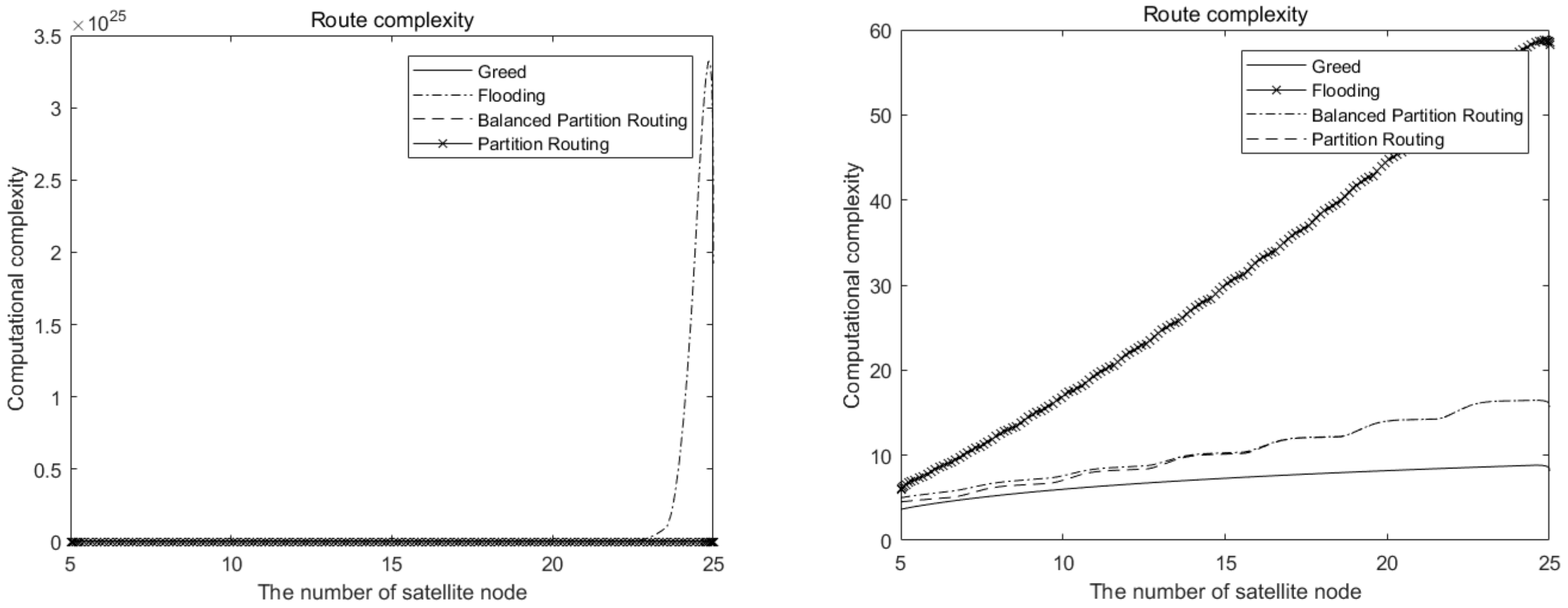
Firstly, the computational complexity of the above algorithm is simulated.
Figure 1 on the left is an actual simulation, and the data on the right are the logarithmic processing. As can be seen from the left figure, with the increase in the number of satellites, the computational complexity of the flooding and backtracking algorithm increases exponentially, while other algorithms increase slowly. From the figure on the right, in general, the flooding and backtracking algorithm has the highest computational complexity, followed by the two partition routing algorithms, and the greedy algorithm has the lowest computational complexity. When the number of inter-star nodes is not very large, the computational complexity of the balanced partition routing algorithm is slightly higher than that of an ordinary partition algorithm.
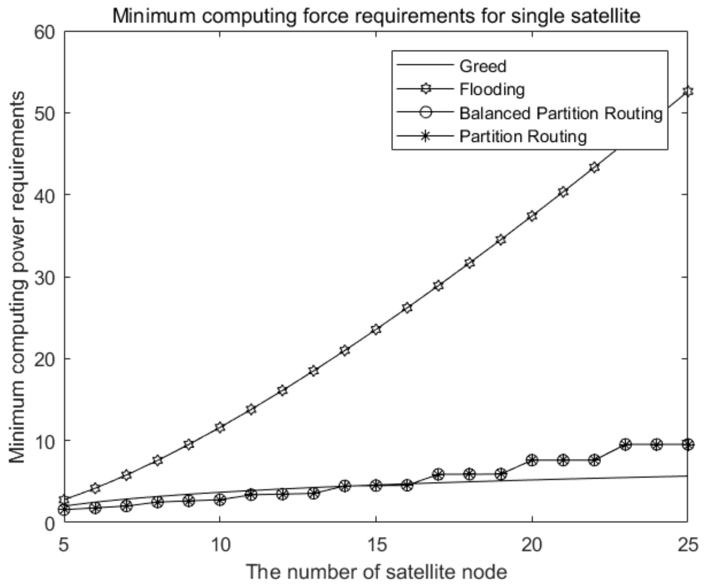
The computation force of a single star node under different algorithms is simulated:
As can be seen from the analysis of Figure 2, with the increase in the number of star nodes in the system, the requirement of the flooding and backtracking algorithm on the computing capacity of a single star node increases rapidly. However, the computing capacity of the two partition routing algorithms increases slowly for a single star node, even approaching the level of a greedy algorithm. This shows that a balanced partition routing algorithm can well distribute computing pressure to multiple star nodes, with stronger destruction resistance and better scalability.
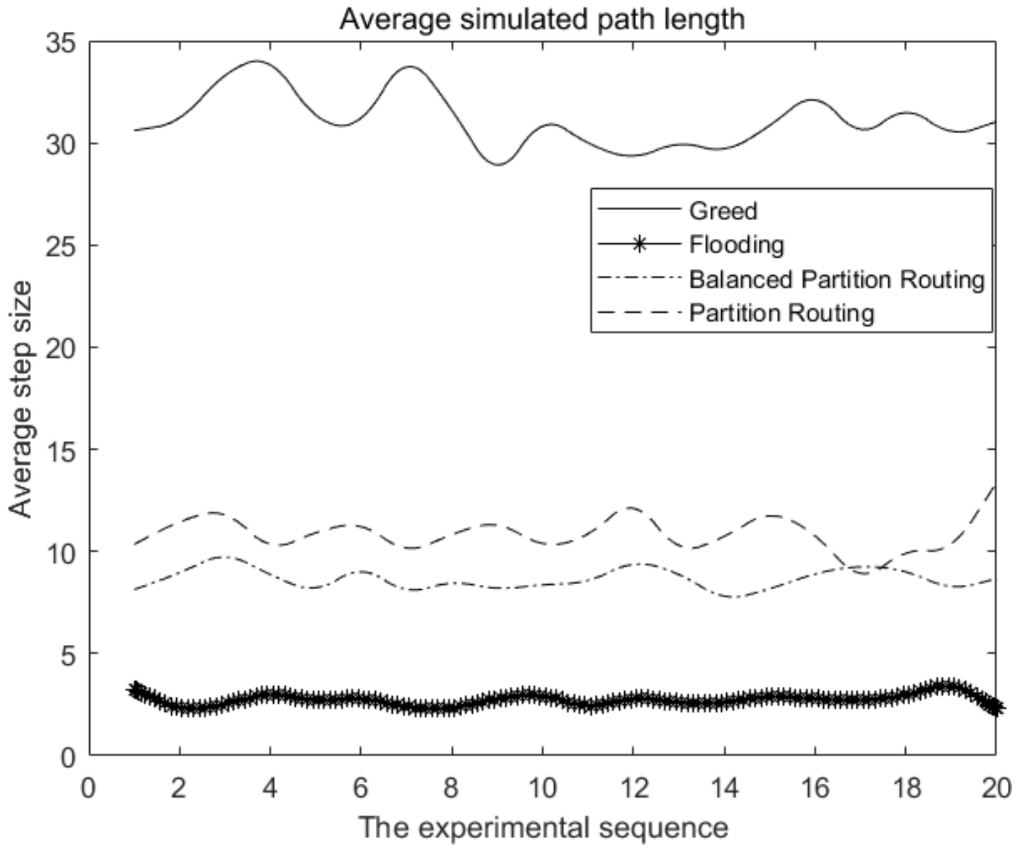
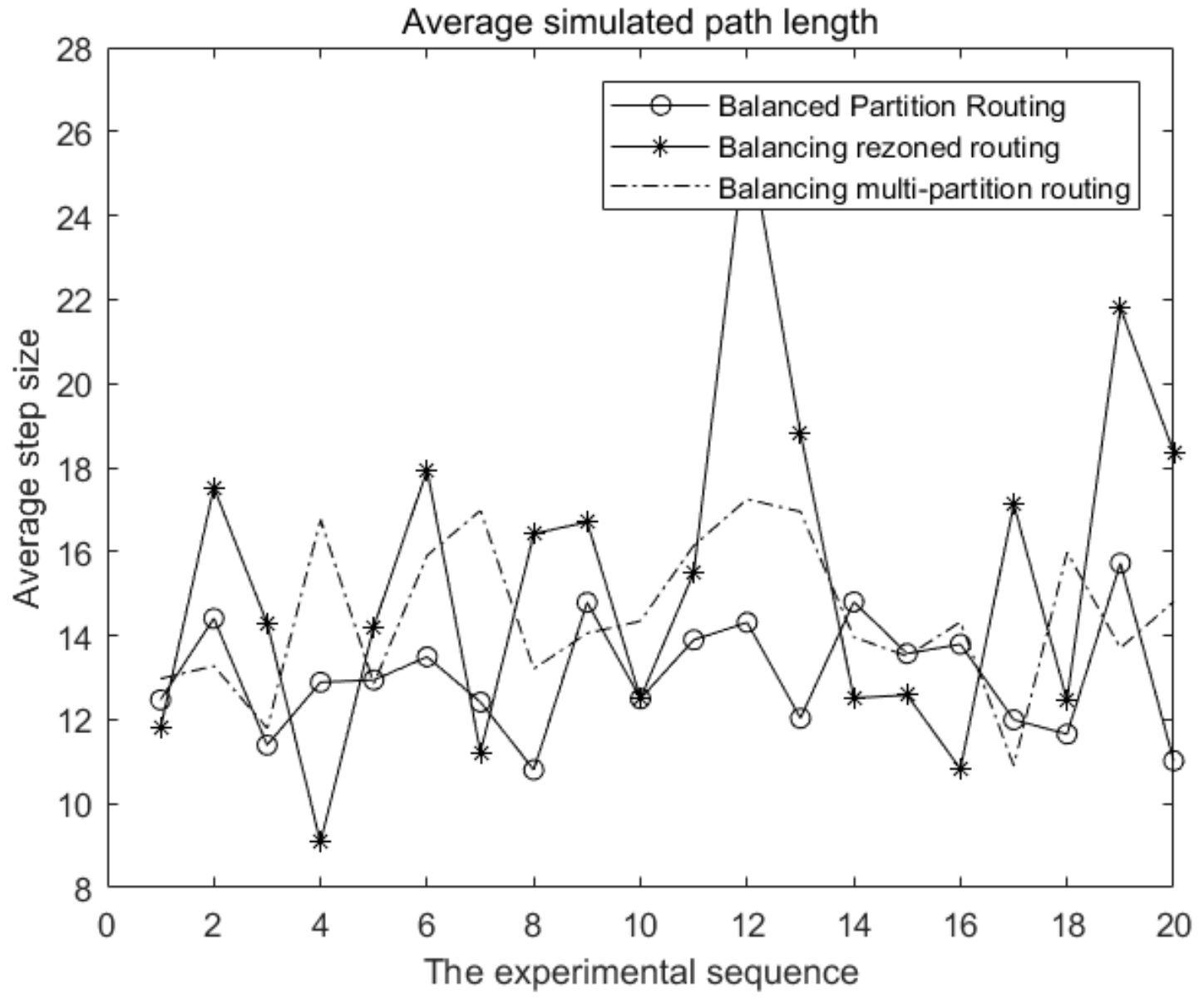
Next, the efficiency of the above algorithms is simulated, and the inter-satellite node number is set to 15.
There were a total of 20 simulations. The average path delay of the greedy algorithm is the highest, and the variance of the average delay in each experiment is large. However, the efficiency of the flooding and backtracking algorithm is relatively stable, and the average delay calculated by this algorithm is significantly less than that of the two partition routing algorithms. Figure 3 shows that the average route length of the balanced partition routing algorithm is shorter than that of the classical partition routing algorithm. In other words, the path calculated by the balanced partition algorithm is better than that of the classical partition routing algorithm.
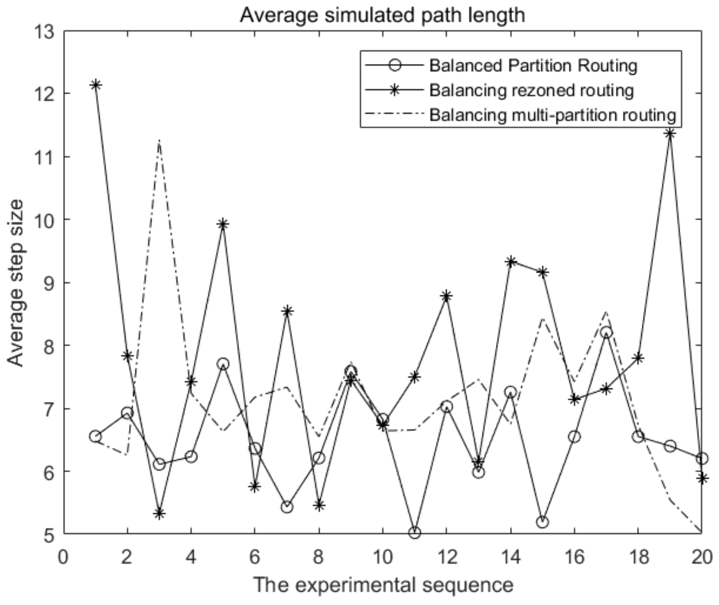
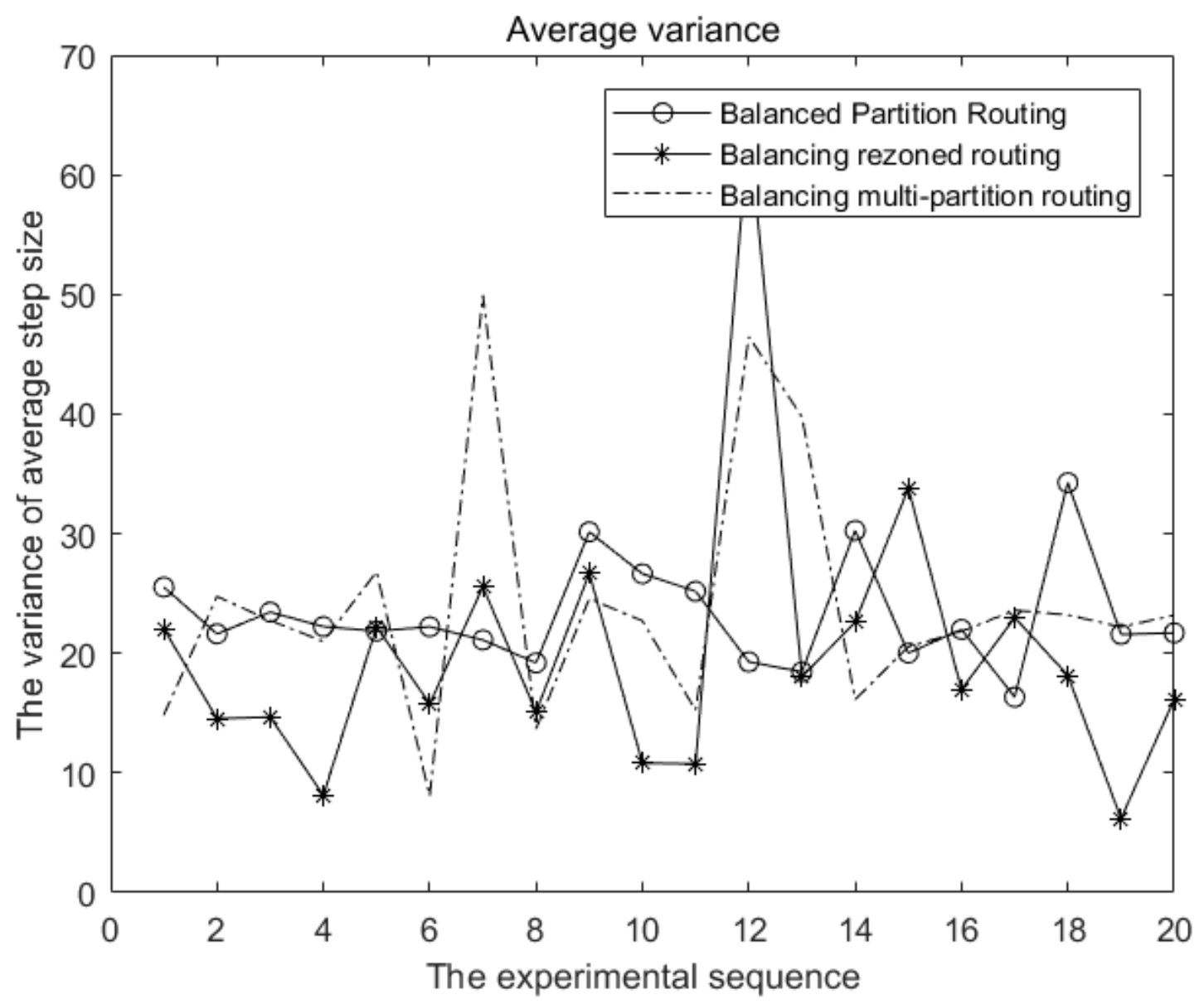
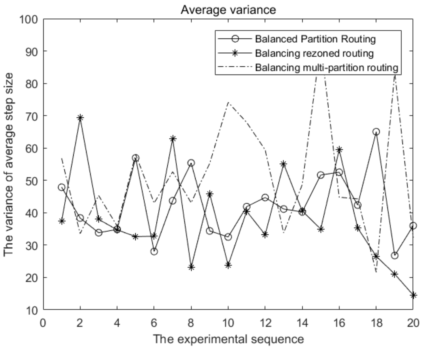
Twenty simulation experiments were conducted here. It can be seen from Figure 4 that the variance of each shortest path length calculated by the flooding and backtracking algorithm is nearly 0, followed by the two partition routing algorithms. The variance calculated by the greedy algorithm is the largest and the stability is the worst. However, considering that the computation complexity of the balanced partition routing algorithm is much lower than that of the flooding and backtracking algorithm, the balanced partition routing algorithm still has high application significance.

3.5. Analysis of Hardware Architecture Cost

The inter-star model is composed of nine star nodes. We randomly conducted 1000 communication missions among these star nodes. We only considered the calculation power consumption of these nodes in calculating the routing path, and the energy consumption of the nodes is positively correlated with the calculation amount. In the actual space environment, the payload of the satellite relies on solar panels to collect solar energy to provide energy.
Table 1 shows the calculation amount for the routing calculation for each node under different algorithms in a simulation experiment. Something that looks like 10 12 or 10 5 is an order of magnitude. The amount of computation here is expressed only in numbers, not in units. The larger the value is here, the greater the amount of computation performed on this node. This means that this node will consume more power and require higher hardware costs. According to the principle of reliability, since we do not know the calculation pressure of each node in advance, the design index of each node should refer to the node with the largest calculation pressure. For example, in this experiment, the design index of the satellite nodes should refer to the No. 1 star under the flooding algorithm, and the No. 6 star under the greedy algorithm. In other words, the actual hardware design cost of satellite nodes is mainly determined by which node bears the most computational pressure.
In order to increase the reliability of the experiment, we conducted a total of 10 experiments. In Table 2, we omit the computation amount of each star node under various algorithms and only show the numerical value of the node with the most computation in each experiment.
It can be seen from this table that the computing capacity requirements of the flooding algorithm for the nodes are not in the same order of magnitude as those of the other three algorithms. If the flooding algorithm is used, the hardware cost for the star nodes will be very large. In theory, the average calculation pressure of each node of the greedy algorithm should be far less than that of the partition routing algorithm and balanced partition routing algorithm. However, each route calculation of the greedy algorithm can only be completed by one node independently and cannot be dispersed to multiple nodes. It leads to great calculation pressure on some nodes. According to our simulation results, the node with the greatest computational pressure of the greedy algorithm is the same order of magnitude as that of the two partition routing algorithms, and the hardware cost among them is also close. From this point of view, on the premise of obtaining extremely high algorithm effectiveness, the hardware cost of a balanced partition routing algorithm is much lower than the flooding algorithm and the cost is close to the greedy algorithm and partition routing algorithm, which have good economic benefits.

4. Optimization of Balanced Partition Routing Algorithm

This section mainly explores the two optimization directions of the balanced partition routing algorithm. As shown in Figure 5, in order to further reduce the calculation pressure of a single node, the balanced partition routing algorithm can further optimize the grouping on the basis of the original grouping. One way is to divide the larger group into smaller groups, each of which belongs to the larger group. This article calls this partitioning method 2. Another method is to divide the original large group into several smaller groups. After the separation, the original large group is cleared. We call it partitioning method 3. This section will explore the calculation pressure of a single node, average path length and variance of average path length under conditions of these two optimization directions.

4.1. Computational Complexity Analysis under Two Partitioning Methods

Method 1: Method 1 here is the balanced partition routing algorithm mentioned above, and its total computational complexity and computation pressure of a single node are shown in Equations (6) and (12).
Method 2: As shown on the left side of Figure 5, all nodes are divided into three large groups, with two small groups inside each large group. To calculate the routing path from star node numbered i to star node numbered j, there may be three cases to consider.
(1)
In the first case, the two star nodes are in the same small group and the routing path is calculated directly in the group.
(2)
In the second case, the two nodes are not in the same small group, but in the same large group. Assuming that the two communication nodes belong to small groups, these two nodes are numbered i + x and j + y, respectively. The communication nodes of each group should be calculated first, and then the paths of these two nodes to their communication nodes should be calculated. Therefore, the total routing path is going to be: i->i+x->j+y->j.
(3)
In the third case, the two nodes are not in the same large group. For node i and node j, the first step is to calculate the communication nodes of large groups that these two nodes i, j, respectively, belong to. Assuming that two large communication nodes are numbered i + m and j + n. Assuming that the two small communication nodes in the large group where node i is located are i + m 1 and i + m 2 . In the same way, we can obtain j + m 1 and j + m 2 and then we have to think about whether i   +   m and i are in the same small group. We also need to consider whether j   +   n and j are in the same group. There are four possibilities:
(3.1)
The first possibility is that node i   +   m and i are in the same small group and node j   +   n and j are also in the same small group. The path in this possibility is going to be: i >   i + m >   j + n >   j .
(3.2)
The second possibility is that node i   +   m and i are not in the same group while node j   +   n and j are in the same group. In this possibility, we need to calculate the routing path from i to i   +   m in the large group firstly and the total routing path is going to be:   i > i + m 1 >   i + m 2 > i + m > j + n > j .
(3.3)
The third possibility is that node i   +   m and i are in the same group while j   +   n and j are not in the same group. The total routing path is: i > i + m > j + n > j +   j + m 1 >   j + m 2 > j .
(3.4)
The last possibility is the exact opposite of the first and its routing path is:   i > i + m 1 >   i + m 2 > i + m > j + n > j + m 1 >   j + m 2 > j .
Minimum computing force requirements for a single node:
C method   2 node N = m = 0 N 12 1 N 6 2 ! N 6 2 m ! + δ 2 + N 6 2 + N 3 2
Total algorithm complexity:
C method   2 N = U 1 + U 2 U 1 = N 6 1 N 1 · m = 0 N 6 2 N 6 2 ! N 6 2 m ! + δ 2 + N 6 N 1 · 2 · m = 0 N 6 2 N 6 2 ! N 6 2 m ! + δ 2 + N 6 2 ) U 2 = N 6 N 1 2 · m = 0 N 6 2 N 6 2 ! N 6 2 m ! + δ 2 + N 3 2 + 2 · 3 · m = 0 N 6 2 N 6 2 ! N 6 2 m ! + δ 2 + N 3 2 + N 6 2 + 4 · m = 0 N 6 2 N 6 2 ! N 6 2 m ! + δ 2 + N 3 2 + 2 · N 6 2
Simplified to obtain:
C method   2 N = N 6 1 N 1 · m = 0 N 6 2 N 6 2 ! N 6 2 m ! + δ 2 + N 6 N 1 · 14 · m = 0 N 6 2 N 6 2 ! N 6 2 m ! + δ 2 + 3 · N 3 2 + 4 · N 6 2
δ 2 = N 6 2 · N 6 2 + δ recall
Method 3: As shown in Figure 5, method 3 is similar to method 1. Nodes in the system are evenly divided into more small groups. All nodes are divided into six groups. To calculate the routing path from star node numbered i to star node numbered j, there may be two cases to consider.
(1)
In the first case, the two star nodes are in the same small group and the routing path is calculated directly in the group.
(2)
In the second case, the two nodes are not in the same group. Assuming that the two communication nodes of the groups these two nodes belong to are numbered i + x and j + y, respectively. Therefore, the total routing path is going to be: i->i+x->j+y->j.
Minimum computing force requirements for a single node:
C method   3 node N = m = 0 N 12 1 N 6 2 ! N 6 2 m ! + N 6 2 + δ 2
Total algorithm complexity:
C method   3 N = N 6 1 N 1 · m = 0 N 12 1 N 6 2 ! N 6 2 m ! + δ 2 + 5 N 6 N 1 · N 6 2 + m = 0 N 12 1 N 6 2 ! N 6 2 m ! + δ 2 · 5 · N 2
Then:
C method   2 N C method   3 node N = N 3 2 > 0
C method   2 N C method   2 N = N 6 1 N 1 · 9 · m = 0 N 6 N 6 2 ! N 6 2 m ! + δ 2 + 3 · N 3 2 N 6 2
Therefore, both the computational complexity of a single node and the total computational complexity of method 2 is greater than that of method 3.

4.2. Algorithm Efficiency Analysis

The inter-star model we selected is composed of 30 star nodes. The data in the Topo table represent the direct distance between stars and satisfy the distribution of μ ,   σ 2 . We explore the actual performance of two balanced partition routing algorithms under different variances. We first simulate the average routing path delay calculated by the two optimization algorithms under different variances and the μ is 5. The simulated data are shown in Table 3.
It can be seen from the above table that we carried out 10 simulation experiments. According to the average value of data obtained from the 10 simulations, the routing path delay calculated by algorithm 1 is the best, algorithm 3 is the second, and algorithm 2 is the worst. In order to eliminate chance, we performed another 20 simulations and drew a simulation graph of the average routing path delay.
Figure 6, Figure 7 and Figure 8 are the simulation diagrams of the actual average route path length calculated by two optimization algorithms with different variances. As can be seen from the figures, an overall trend is that with the increase in data variance in the Topo table, the average path length calculated by the three algorithms increases. However, in terms of internal comparison, the average path length obtained by algorithm 1 is the shortest, while that obtained by algorithm 2 is the longest.
As can be seen from the Table 3 and Table 4, as the variance of data in the Topo table increases, so does the variance of the average path length calculated by each algorithm. Internally, under the same conditions, the variance of the average path length calculated by algorithm 2 is the smallest, indicating that the path length calculated by algorithm 2 for each routing path is relatively close, and the efficiency of the algorithm is the most stable. Figure 9, Figure 10 and Figure 11 also reflect the same results. In practical applications, such algorithms are more resistant to destruction. If the lengths of different paths calculated differ greatly, some star nodes will be overloaded while others are idle, which wastes resources and reduces the efficiency of inter-star communication [24].

4.3. Analysis of Hardware Architecture Cost

The inter-star model is composed of 18 star nodes. Other experimental details and methods are exactly the same as the simulation experiment in 3.5. Table 5 shows the calculation amount of routing calculation for each node under three algorithms in a simulation experiment.
Table 5 shows the calculation power consumption of each star node under various algorithms in the first experiment. Table 6 reflects the node with the highest calculated pressure in the 10 experiments. It can be seen from the two tables that the computational pressure borne by each node under these three algorithms is relatively average, which means that each node was fully utilized. To be specific, the average and maximum computational pressures borne by each node of the two algorithms after optimization are indeed significantly lower than those before optimization, which proves that the two optimization directions can further reduce hardware costs.

5. Conclusions

This paper proposes a new inter-satellite balanced partition routing algorithm. Firstly, the total computation complexity and single node’s pressure of the algorithm and other traditional algorithms are analyzed from the point of view of mathematics. The simulation model is built to simulate the performance of the four inter-satellite routing algorithms, including average path propagation delay, the variance of the path propagation delay, and the calculated pressure of a single node. Simulation results reveal that compared with other algorithms, the proposed balanced partition routing algorithm achieves better performance.
In the latter part of this paper, two further optimization directions of a balanced partition routing algorithm are analyzed. Firstly, experimental results show that these two optimization methods can further reduce the complexity of the algorithm. Moreover, the hardware cost of nodes is greatly reduced. Finally, the further optimization of the balanced partition routing algorithm can adapt to various scenarios and has good mobility. This algorithm could not only be used as an alternative scheme in the routing planning of low-orbit micro-satellite constellations and star links but also be used as a general scheme for decentralized data fusion in cooperative systems such as unmanned aerial vehicle formations.
In our following work, we intend to study the grouping of balanced partition routing algorithms. In our branch of experimental study, we found that the average path delay calculated by different grouping methods is huge for the balanced partition routing algorithm. The good grouping method will greatly improve the efficiency of the algorithm. On the other hand, the processing delay of data within the nodes will also be considered in our future research [1].

Author Contributions

Conceptualization, Z.X., Z.J. and X.J.; Formal analysis, Z.X. and Z.J.; Methodology, H.C. and X.G.; Resources, J.Y. and K.X.; Software, H.C. and X.G.; Validation, H.C. and S.L.; Writing—original draft, H.C.; Writing—review and editing, H.C. and Z.X. All authors have read and agreed to the published version of the manuscript.

Funding

This research was funded by National Natural Science Foundation of China grant number 62073289.

Data Availability Statement

Not applicable.

Conflicts of Interest

The authors declare no conflict of interest.

Abbreviations

The following abbreviations are used in this manuscript:
NNumber of satellite nodes in the system
TopoA table storing direct distances between stars
No. Satellite identification
a i j Direct distance from the No. i to the No. j satellite
μ Average of the data in Topo table
σ 2 Variance of the data in Topo table
φ A group
G C omputational complexity of Greedy algorithm
F C omputational complexity of Flooding algorithm
δ 1 Cost of backtracking part of the Flooding algorithm
P C omputational complexity of Partition routing algorithm
δ 2 Cos t   of   δ recall +   δ greed
δ recall Cost of backtracking part of Partial Flooding algorithm
δ greed Overhead of the greedy algorithm in the group
C C omputational complexity of Balanced partition routing algorithm
G node Calculated pressure of a node in Greedy algorithm
F node Calculated pressure of a node in Flooding algorithm
P node Calculated pressure of a node in Partial Flooding algorithm
C node Calculated pressure of a node in of Balanced partition routing algorithm
G p a t h Average path length of Greedy algorithm
F p a t h Average path length of Flooding algorithm
P p a t h Average path length of Partial Flooding algorithm
C p a t h Average path length of Balanced partition routing algorithm
C m e t h o d   2 n o d e Calculated pressure of a node in of Balanced partition routing algorithm (2)
C m e t h o d   3 n o d e Calculated pressure of a node in of Balanced partition routing algorithm (3)
C m e t h o d   2 Average path length of Balanced partition routing algorithm (2)
C m e t h o d   3 Average path length of Balanced partition routing algorithm (3)

References

  1. Alishahi, M.; Hajiabolhassan, H. On chromatic number and minimum cut. J. Comb. Theory Ser. B 2019, 139, 27–46. [Google Scholar] [CrossRef] [Green Version]
  2. Balas, E.; Yu, C.S. Finding a Maximum Clique in an Arbitrary Graph. SIAM J. Comput. 1986, 15, 1054–1068. [Google Scholar] [CrossRef]
  3. Bondy, J.A.; Murty, U.S.R. Graph Theory; Springer: New York, NY, USA, 2008. [Google Scholar]
  4. Bonomo, F.; Cornaz, D.; Ekim, T.; Ries, B. Perfectness of clustered graphs. Discret. Optim. 2013, 10, 296–303. [Google Scholar] [CrossRef]
  5. Kergosien, Y.; Lenté, C.; Billaut, J.-C.; Perrin, S. Metaheuristic algorithms for solving two interconnected vehicle routing problems in a hospital complex. Comput. Oper. Res. 2013, 40, 2508–2518. [Google Scholar] [CrossRef]
  6. Chen, J.; Liu, S.; Zhang, Y. Inter-Satellite Token Ring Ad Hoc Network Technology for Micro-Nano Satellite Cluster Collaboration. In Proceedings of the 2021 3rd International Conference on Advances in Computer Technology, Information Science and Communication (CTISC), Shanghai, China, 23–25 April 2021; pp. 125–131. [Google Scholar] [CrossRef]
  7. Dong, C.; Xu, X.; Liu, A.; Liang, X. Load balancing routing algorithm based on extended link states in LEO constellation network. China Commun. 2022, 19, 247–260. [Google Scholar] [CrossRef]
  8. Chen, Q.; Giambene, G.G.; Yang, L.; Fan, C.; Chen, X. Analysis of Inter-Satellite Link Paths for LEO Mega-Constellation Networks. IEEE Trans. Veh. Technol. 2021, 70, 2743–2755. [Google Scholar] [CrossRef]
  9. Weng, Y.; Liu, L. On-demand partial topology routing algorithm in LEO satellite networks. Comput. Eng. Appl. 2007, 43, 148–150. [Google Scholar]
  10. Henderson, T.H.; Katz, R.H. On Distributed and Geographic-Based Packet Routing for LEO Satellite Networks. In Proceedings of the Globecom ‘00—IEEE. Global Telecommunications Conference. Conference Record (Cat. No.00CH37137), San Francisco, CA, USA, 27 November–1 December 2000; Volume 2, pp. 1119–1123. [Google Scholar]
  11. Ekici, E.; Akyildiz, I.F.; Bender, M.D. A Distributed Routing Algorithm for Data gram Traffic in LEO Satellite Networks. IEEE J. Sel. Areas Commun. 2004, 22, 272–286. [Google Scholar]
  12. Woo, S.; Ohara, M.; Torrie, E.; Singh, J.; Gupta, A. The SPLASH-2 programs: Characterization and methodological considerations. In Proceedings of the 22nd annual international symposium on Computer architecture—ISCA ’95, Santa Margherita Ligure, Italy, 22–24 June 1995; pp. 24–36. [Google Scholar]
  13. Bienia, C.; Kumar, S.; Singh, J.P.; Li, K. The Parsec Benchmark Suite: Characterization and Architectural Implications. In Proceedings of the 17th International Conference on Parallel Architectures and Compilation Techniques, Toronto, ON, Canada, 25–29 October 2008; pp. 72–81. [Google Scholar]
  14. Bienia, C.; Kumar, S.; Li, K. PARSEC vs. SPLASH-2: A quantitative comparison of two multithreaded benchmark suites on Chip-Multiprocessors. In Proceedings of the IEEE International Workshop/Symposium on Workload Characterization, Seattle, WA, USA, 14–16 September 2008; pp. 47–56. [Google Scholar] [CrossRef] [Green Version]
  15. Patel, A.; Ghose, K. Energy-Efficient Mesi Cache Coherence with Pro-Active Snoop Filtering for Multicore Microprocessors. In Proceedings of the 13th international symposium on Low power electronics and design, Bangalore, India, 11–13 August 2008; pp. 247–252. [Google Scholar]
  16. Zeng, G.; Zhan, Y.; Pan, X. Failure-Tolerant and Low-Latency command in Mega-Constellations: The Redundant Multi-Path Routing. IEEE Access 2021, 9, 34975–34985. [Google Scholar] [CrossRef]
  17. Martin, M.M.K.; Sorin, D.J.; Beckmann, B.M.; Marty, M.R.; Xu, M.; Alameldeen, A.R.; Moore, K.E.; Hill, M.D.; Wood, D.A. Multifacet’s general execution-driven multiprocessor simulator (GEMS) toolset. ACM SIGARCH Comput. Arch. News 2005, 33, 92–99. [Google Scholar] [CrossRef]
  18. Yang, J.; Li, D.; Jiang, X.; Chen, S.; Hanzo, L. Enhancing the Resilience of Low Earth Orbit Remote Sensing Satellite Networks. IEEE Netw. 2020, 34, 304–311. [Google Scholar] [CrossRef]
  19. Zheng, B.; Yen, K.; Peng, X.; Zhang, R. Angle Partition-Based TDMA for VDES Satellite Multiuser Downlink Communications. In Proceedings of the GLOBECOM 2020—2020 IEEE Global Communications Conference, Taipei, Taiwan, 7–11 December 2020; pp. 1–6. [Google Scholar]
  20. Yang, K.; Zhang, B.; Guo, D. Controller and Gateway Partition Placement in SDN-Enabled Integrated Satellite-Terrestrial Network. In Proceedings of the 2019 IEEE International Conference on Communications Workshops (ICC Workshops), Shanghai, China, 20–24 May 2019; pp. 1–6. [Google Scholar]
  21. Ebrahimi, M.; Daneshtalab, M.; Farahnakian, F.; Plosila, J.; Liljeberg, P.; Palesi, M.; Tenhunen, H. HARAQ: Congestion-Aware Learning Model for Highly Adaptive Routing Algorithm in On-Chip Networks. In Proceedings of the 2013 ACM/IEEE International Workshop on System Level Interconnect Prediction (SLIP), Austin, TX, USA, 2 June 2013; pp. 19–26. [Google Scholar] [CrossRef]
  22. Dehyadegari, M.; Daneshtalab, M.; Ebrahimi, M.; Plosila, J.; Mohammadi, S. An adaptive fuzzy logic-based routing algorithm for networks-on-chip. In Proceedings of the 2011 NASA/ESA Conference on Adaptive Hardware and Systems (AHS), San Diego, CA, USA, 6–9 June 2011; pp. 208–214. [Google Scholar] [CrossRef]
  23. Ebrahimi, M.; Daneshtalab, M.; Liljeberg, P.; Plosila, J.; Tenhunen, H. Exploring partitioning methods for 3D Networks-on-Chip utilizing adaptive routing model. In Proceedings of the Fifth IEEE/ACM International Symposium on Networks on Chip, Pittsburgh, PA, USA, 1–4 May 2011; pp. 73–80. [Google Scholar] [CrossRef] [Green Version]
  24. Wang, L.; Jin, Y.; Kim, H.; Kim, E.J. Recursive partitioning multicast: A bandwidth-efficient routing for Networks-on-Chip. In Proceedings of the 2009 3rd ACM/IEEE International Symposium on Networks-on-Chip, Washington, DC, USA, 10–13 May 2009; pp. 64–73. [Google Scholar] [CrossRef] [Green Version]
Figure 1. Simulation of computational complexity of three algorithms.
Futureinternet 14 00207 g001
Figure 2. Simulation of calculated pressure for a single node.
Futureinternet 14 00207 g002
Figure 3. Simulation of average path length for four algorithms.
Futureinternet 14 00207 g003
Figure 4. Simulation of the variance of average path length for four algorithms.
Futureinternet 14 00207 g004
Figure 5. Two kinds of optimized partitioning (method 2 is left, method 3 is right).
Futureinternet 14 00207 g005
Figure 6. Simulation of average path length ( μ = 5 , σ 2 = 5 ).
Futureinternet 14 00207 g006
Figure 7. Simulation of average path length ( μ = 5 , σ 2 = 10 ).
Futureinternet 14 00207 g007
Figure 8. Simulation of average path length ( μ = 5 , σ 2 = 15 ).
Futureinternet 14 00207 g008
Figure 9. Simulation of the variance of average path length ( μ = 5 , σ 2 = 5 ).
Futureinternet 14 00207 g009
Figure 10. Simulation of the variance of average path length ( μ = 5 , σ 2 = 10 ).
Futureinternet 14 00207 g010
Figure 11. Simulation of the variance of average path length ( μ = 5 , σ 2 = 15 ).
Futureinternet 14 00207 g011
Table 1. Amount of computation for each node.
Satellite Number123456789
Types of Algorithms
Flooding   ( 10 12 )13.041.752.891.285.388.572.254.119.51
Greedy   ( 10 4 ) 0.092.731.001.991.3421.912.82.372.62
Partition   routing   ( 10 5 ) 6.116.365.227.315.456.266.216.326.25
Balanced   partition   routing   ( 10 5 ) 7.627.707.717.677.887.637.677.647.60
Table 2. Largest amount of computation for single node in each experiment.
Types of Algorithms Greedy 10 5 Flooding 10 12 Partition   Routing 10 5 Balanced   Partition   Routing ( 10 5 )
Sequence
12.1913.047.317.88
21.219.636.297.99
37.419.996.388.06
43.533.926.728.09
51.751.266.028.08
66.442.575.988.16
75.3219.95.688.14
88.013.786.488.18
92.112.826.468.28
101.076.116.188.22
Table 3. Data of simulated time average path cost.
Conditions μ = 5 ,   σ 2 = 6 μ = 5 , σ 2 = 10 μ = 5 ,   σ 2 = 15
Sequence Algorithm 1Algorithm 2Algorithm 3Algorithm 1Algorithm 2Algorithm 3Algorithm 1Algorithm 2Algorithm 3
16.97277.55657.77218.987111.742511.111913.347419.548712.4728
27.00347.11665.85308.57448.93007.921214.434317.562515.6544
36.31846.11107.37428.63169.885713.319311.970515.714111.0548
46.72298.00886.39719.451810.989010.887612.940716.188318.7025
56.80027.80506.97288.030312.543511.877114.055020.227612.5364
66.35986.63429.627510.042713.61408.853015.177518.293714.5067
76.430010.38928.06009.3336515.34809.507211.238214.744510.6957
86.51927.70346.97289.003014.718110.766412.399211.962615.5931
96.54778.16797.88209.541912.886611.858915.350921.436021.0220
106.43577.78897.78138.109511.390910.662913.102912.52839.7106
average6.6117.7287.4698.97112.20510.67713.40216.82114.195
Notation: The units of the metrics in this table are second(s).
Table 4. Data of variance of simulated time average path cost.
Conditions μ = 5 ,   σ 2 = 6 μ = 5 , σ 2 = 10 μ = 5 ,   σ 2 = 15
Sequence Algorithm 1Algorithm 2Algorithm 3Algorithm 1Algorithm 2Algorithm 3Algorithm 1Algorithm 1Algorithm 1
117.839519.163214.894128.262442.790957.411889.317063.374672.3029
220.127318.532528.246939.247419.006339.174391.882079.7508104.3368
316.174116.351926.075147.530336.643051.372585.577452.7638124.6169
414.261212.063121.418144.612936.241548.476080.269655.081184.7636
518.300812.654715.671246.558532.772063.515794.905789.132485.5036
626.048817.134021.139341.622723.047535.692984.249652.8075102.9034
713.586014.028720.769330.391234.661950.890982.992597.9406131.0594
819.641015.038317.703834.520723.541966.323396.125056.642896.4693
917.294223.970122.557640.651248.151744.165554.013073.5422108.1908
1019.761714.421433.984854.409843.630350.878890.856549.9056126.0783
average18.30316.33622.46040.78134.04950.79085.01967.095103.623
Notation: The units of the metrics in this table is s 2 .
Table 5. Amount of computation for each node.
Satellite Number123456789
Types of Algorithms 101112131415161718
Method 1   ( 10 6 ) 1.831.851.901.931.821.961.931.871.85
1.841.901.841.861.901.881.901.881.85
Method 2   ( 10 5 ) 4.744.945.125.325.374.994.955.185.11
5.175.174.725.125.004.864.875.274.85
Method 3   ( 10 5 ) 6.056.196.376.176.206.086.346.186.23
6.086.266.216.066.186.136.186.156.15
Table 6. Largest amount of computation for single node in each experiment.
Types of Algorithms Method   1 ( 10 6 ) Method   2 ( 10 5 ) Method   3 ( 10 5 )
Sequence
11.965.376.37
22.025.466.34
32.075.486.39
42.065.236.51
52.105.306.14
62.045.386.20
72.085.266.41
82.085.476.30
92.025.876.34
102.065.306.22
Publisher’s Note: MDPI stays neutral with regard to jurisdictional claims in published maps and institutional affiliations.

