Article

Handover Management in 5G Vehicular Networks

by
Ioannis Kosmopoulos
1,†,
Emmanouil Skondras
1,†,
Angelos Michalas
2,†,
Emmanouel T. Michailidis
3,*,† and
Dimitrios D. Vergados
1,†
1
Department of Informatics, University of Piraeus, 80 Karaoli & Dimitriou Str., 18534 Piraeus, Greece
2
Department of Electrical and Computer Engineering, University of Western Macedonia, Karamanli & Ligeris, 50131 Kozani, Greece
3
Department of Electrical and Electronics Engineering, University of West Attica, Ancient Olive Grove Campus, 250 Thivon & P. Ralli Str., 12241 Egaleo, Greece
*
Author to whom correspondence should be addressed.
These authors contributed equally to this work.
Future Internet 2022, 14(3), 87; https://doi.org/10.3390/fi14030087
Submission received: 23 February 2022 / Revised: 10 March 2022 / Accepted: 11 March 2022 / Published: 13 March 2022
(This article belongs to the Special Issue Future Intelligent Vehicular Networks toward 6G)

Abstract

:
Fifth-Generation (5G) vehicular networks support novel services with increased Quality of Service (QoS) requirements. Vehicular users need to be continuously connected to networks that fulfil the constraints of their services. Thus, the implementation of optimal Handover (HO) mechanisms for 5G vehicular architectures is deemed necessary. This work describes a scheme for performing HOs in 5G vehicular networks using the functionalities of the Media-Independent Handover (MIH) and Fast Proxy Mobile IPv6 (FPMIP) standards. The scheme supports both predictive and reactive HO scenarios. A velocity and alternative network monitoring process prepares each vehicle for both HO cases. In the case of predictive HO, each time the satisfaction grade of the vehicular user drops below a predefined threshold, the HO is initiated. On the other hand, in the case of reactive HO, the vehicle loses the connectivity with its serving network and connects to the available network that has obtained the higher ranking from the network selection process. Furthermore, the HO implementation is based on an improved version of the FPMIPv6 protocol. For the evaluation of the described methodology, a 5G vehicular network architecture was simulated. In this architecture, multiple network access technologies coexist, while the experimental results showed that the proposed scheme outperformed existing HO methods.

Graphical Abstract

1. Introduction

Fifth-generation (5G) vehicular networks have emerged rapidly. In a typical 5G vehicular network architecture, vehicular equipment includes On-Board Units (OBUs) [1] and mobile User Equipment (UEs). Vehicles communicate with each other, as well as with access network infrastructures. Access networks usually construct a Fog [2] infrastructure, which interacts with a Cloud environment, offering vehicular services. Many vehicular users can be served from each vehicle, while each user can simultaneously use multiple services with different constraints with each other.
In this network environment, increased communication requirements are arising for the vehicular users and, thus, an increased number of network access resources is needed. To address this issue, the technology of Ultra-Dense Networking (UDN) [3,4] indicates that dense 5G access network infrastructures can be implemented, where an increased number of Points of Access (PoAs) can provide plenty of communication resources to users [5,6]. Regarding the operational principles of UDN, several different technologies can coexist in the network access environment. Indicatively, the Macrocells and Femtocells that construct the network access environment can implement technologies such as the IEEE 802.11p Wireless Access for Vehicular Environment (WAVE) [7], the 3GPP Long-Term Evolution Advanced (LTE-A) [8], and the IEEE 802.16 Worldwide Interoperability for Microwave Access (WiMAX) [9]. Furthermore, regarding the design principles of the 5G Core (5GC) [10], the core network of a 5G vehicular architecture applies virtualization techniques for resource manipulation, including network slicing [11] and mobility management [12]. Communication among virtual network functionalities is achieved using RESTful application programming interfaces (RESTful APIs) [13] over HTTPS-/JSON-based protocols [14]. As a result, the implementation of novel network manipulation algorithms becomes independent of the specific underlying hardware optimizing the support for heterogeneous network technologies.
The co-existence of heterogeneous wireless access technologies indicates the need for efficient manipulation of the vehicles’ mobility. This need has involved the employment of the IEEE Media Independent Handover (MIH) and the Fast Proxy Mobile IPv6 (FPMIPv6) standards [15] for the mobility transfer. Specifically, the MIH protocol defines HO operations across different access networks. Its architecture provides generic interfaces and primitives independent of the type of vehicular equipment and access networks, supporting link-layer events and network information retrieval. On the other hand, two reference HO scenarios are introduced in FPMIPv6, the predictive and the reactive scenario, depending on the vehicle’s speed. In the predictive scenario, the vehicle before disconnecting from its previous network sends a handover indication report to its Mobility Access Gateway (MAG) [16] declaring the new network, which is selected as the target for performing the HO. In case the vehicle connects to the new network without informing of its MAG in the previous network, the reactive operation of FPMIPv6 is performed.
Vehicles should always be connected to the most appropriate access network to fulfil the QoS constraints of their services. To address this issue, Multi-Attribute Decision-Making (MADM) algorithms can be applied to select the best alternative among candidate networks by taking into consideration a set of evaluation criteria. Well-known methodologies include the Analytic Hierarchy Process (AHP) [17], the Analytic Network Process (ANP) [18], Simple Additive Weighting (SAW) [17,19], Fuzzy SAW (FSAW) [20], Multiplicative Exponential Weighting (MEW) [17] and the Technique for Order Preference by Similarity to Ideal Solution (TOPSIS) [21].
This paper describes a methodology for supporting Handovers (HOs) on 5G vehicular networks. Both predictive and reactive HO modes are supported. During the vehicles movement, a velocity and alternative network monitoring process executes. This process applies the Mobility State Estimation (MSE) technique of the LTE [22], which was improved in [23], in order to facilitate the decision process by taking into consideration that both Macrocells and Femtocells can serve the territory of each vehicle. Thus, the vehicle’s velocity is continuously monitored and characterized as Normal, Medium, or High, considering the number of HOs performed by the vehicle during a sliding time window [23]. Furthermore, it ranks the candidate networks by taking into consideration the vehicle’s velocity, network characteristic criteria, provider policy criteria, and energy-aware criteria. Specifically, if the vehicle’s velocity is Normal, all the networks, including both Macrocells and Femtocells, are considered as network alternatives. On the other hand, if the vehicle’s velocity is Medium, some Femtocells along the vehicle’s trajectory are skipped, in order for the HO rate to be reduced. Finally, if the vehicle’s velocity is High, only the available Macrocells are considered as network alternatives. Moreover, in the predictive HO scenario, each time that the grade of the user satisfaction drops below a predefined threshold, the HO is initiated and the process of the network selection is performed. Correspondingly, in the reactive HO operation, whenever the vehicular user loses the connectivity with his/her serving network, it connects to the available network that obtained the higher ranking during the network selection process.
The discussed scheme implements several characteristics, including:
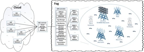
  • The HO management services, namely the velocity and alternative network monitoring, the HO initiation, the network selection, and the HO execution are performed at the Fog and the Cloud infrastructures to reduce the workload at the vehicle;
  • Both predictive and reactive HOs modes are supported for the mobility transfer;
  • The vehicle’s velocity is considered in order for unnecessary HOs to short-range cells (such as Femtocells) to be avoided, since a vehicle that moves with high velocity will remain for a short time period inside their coverage area;
  • HO initiation is performed by taking into consideration the user satisfaction, which is estimated using both the Signal-to-Noise-plus-Interference (SINR) and the perceived Quality of Service (QoS) parameters, due to the fact that users that perceive a good SINR may not be satisfied by the QoS that they also perceive from their current networks;
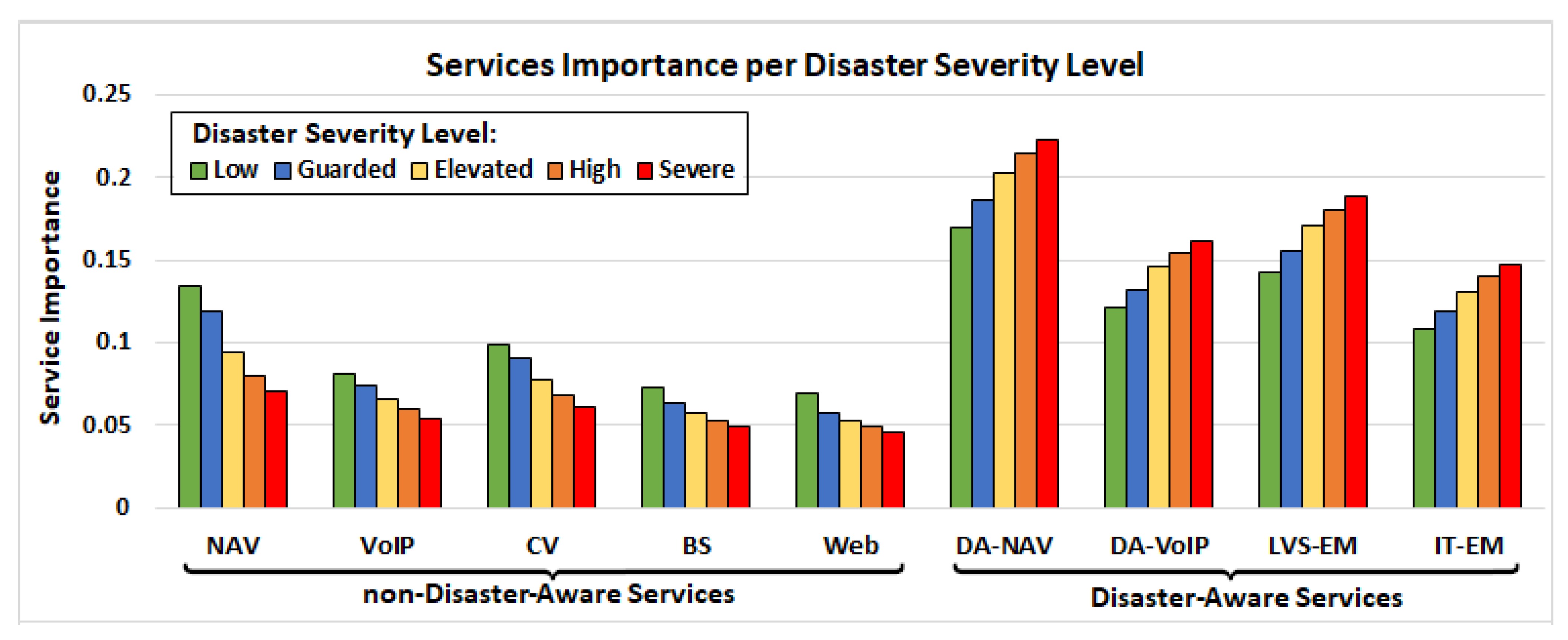
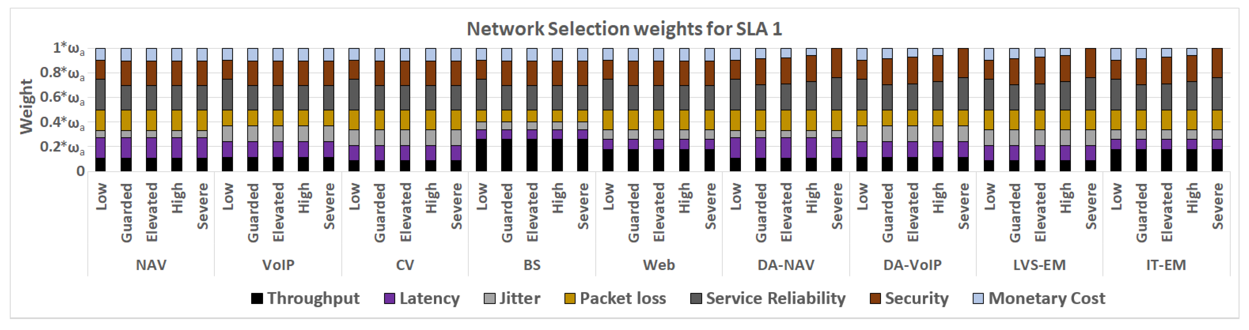
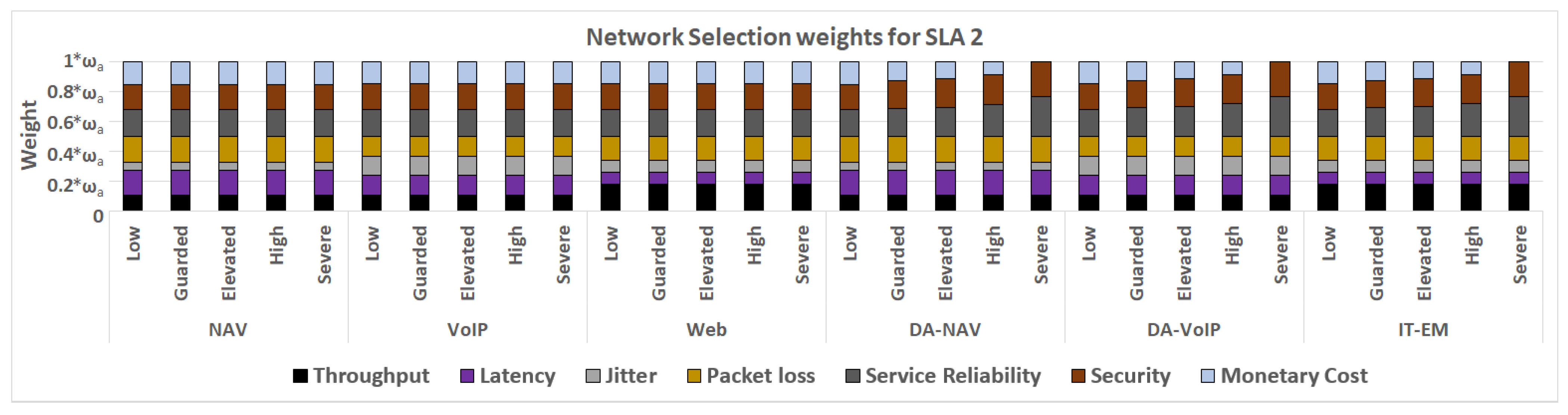
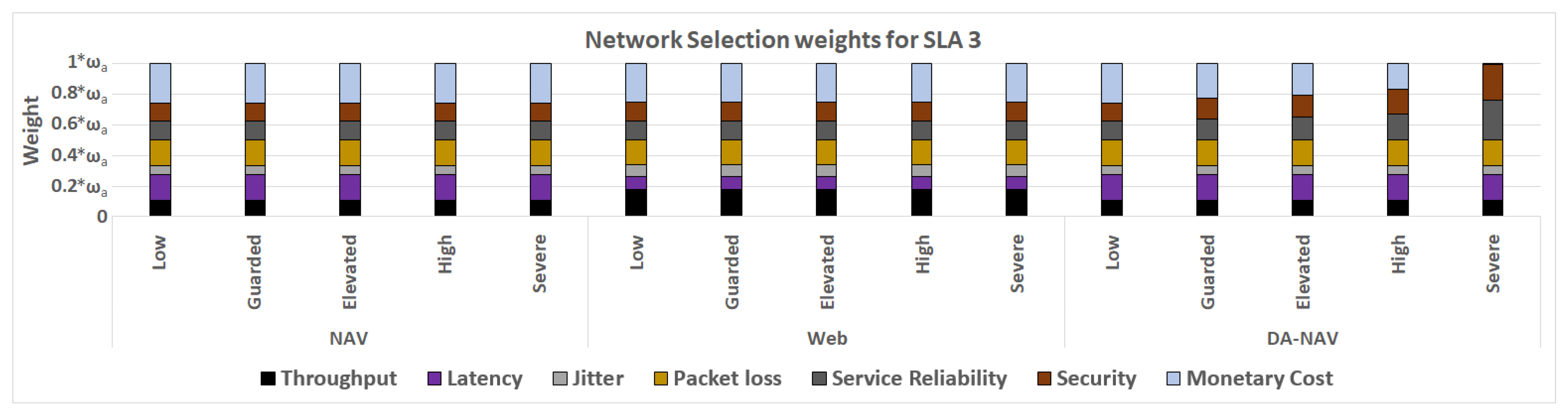
  • Network selection takes into consideration contradictory criteria for different application types and users’ SLAs to satisfy the requirements of demanding services;
  • The HO scheme applies an improved version of the MIH framework and the FPMIPv6 protocol.
The remainder of the paper is organized as follows: In Section 2, the related research literature is revised. Section 3 describes the proposed HO scheme, and Section 4 presents the implemented signaling process. Subsequently, Section 5 presents the simulation setup and the experimental results. Finally, Section 6 concludes the discussed work.

2. Related Work

In general, the HO process usually consists of the HO initiation, the network selection, and the HO execution subprocesses. Several HO schemes have been proposed in the research literature supporting the above network management functions.
In [24], the authors introduced the necessity of Quality of Service (QoS) and Quality of Experience (QoE) parameters in mobility management algorithms. In this approach, a QoE algorithm for video streaming in 5G vehicular networks (HoVe) is proposed in order to improve the overall handover performance. The Analytic Hierarchy Process (AHP) technique is used to identify the importance of the current metrics including radio resources, vehicle’s mobility, QoE. etc. The Structural Similarity (SSIM) is evaluated as a QoE metric estimating the corruption between the original and the transmitted video. The proposed algorithm outperforms the standard LTE RSSI-based algorithm [25] for video services.
In [26], the authors proposed an HO triggering scheme based on dynamic criteria. An important aspect of the handover process is the momentum of the trigger event, which initiates the HO. An imprecise trigger could produce service interruptions, data loss, latency, and radio-link failure. The proposed scheme benefits from the IEEE 802.21 Media Independent Handover (MIH) and its services, introducing the link going down event. A dynamic value is calculated to adjust the trigger point during the handover delivery time according to the mobile node’s current speed.
In [27], the authors presented a machine learning technique to predict the necessity of a handover so as to maintain the users’ QoE. The proposed method makes use of a support vector regression algorithm (SVR) to evaluate an HO score periodically per mobile node. The algorithm obtains the signal strength, the throughput, and the previous handover score of the node as the input criteria. The mobile node is triggered to perform the HO to a new network in case its handover cost is above a threshold specified by the system policy.
In [28], an MIH-enhanced FPMIPv6 methodology was proposed. In particular, the functionalities of the Evolved Packet Core (EPC) [29] were considered, while a scheme that implements the IEEE 802.11 MIH protocol in the EPC architecture for performing seamless HO was described. Additionally, the use of a transient flag was proposed for eliminating both the ping-pong effect and false HOs by retaining the initial and transient bindings at the LMA.
In [30], the Predictive Handover Mechanism for Video streaming in cloud-based urban VANET (PHMVV) method was proposed considering a list of alternative Points of Access (PoAs). The PHMVV takes into account parameters such as the velocity of the vehicle, its distance from each PoA, its moving direction, and the link quality of each PoA. Accordingly, when the vehicle approaches an alternative PoA with better link quality than that of its current PoA, the vehicle performs an HO to it.
In [31], the Mobility-Aware Handover scheme for Smart Cities Environment (MAH-SCE) was described. In particular, road traffic conditions were gathered from a Smart City [32] environment using sensors. An HO initiation mechanism initiates an HO considering the road traffic, as well as the SNR that the vehicle perceives from its current PoA. Additionally, in order to reduce the HO rate, Femtocells are not considered as network alternatives when the vehicle’s velocity is above 16 m/s. However, it has to be noted that the authors did not provide an adequate explanation about the selection of this specific threshold value. However, an adequate explanation about the selection of this specific threshold value was provided in [31]. Therefore, in our work, the vehicle’s velocity was also monitored and a different approach to this task was implemented by considering the operation principles of the LTE MSE technique [22].
In [33], the Mobility-Aware Handover in Ultra-Dense Vehicular Environment (MAH-UDVE) method was proposed. The direction to which each vehicle moves is considered for the most appropriate PoA to be selected. Specifically, the vehicle’s mobility is analyzed in order for a set of network alternatives to be created. Regarding the target network to perform the HO, three options were assessed including the network cell, the next cell in the same or opposite direction of the vehicle, and the cell with the lowest load.
In [34], the Context-Aware Load Balancing (HO-CALB) mobility management scheme was proposed. HO-CALB is applied to a network architecture where both WiFi and WiMAX networks coexist. When the QoS that each user perceives drops below a predefined threshold, an HO will be initiated. Thereafter, during the network selection, the data traffic load is distributed to WiMAX and WiFi PoAs by taking into consideration the available bandwidth of each one.
In [35], the Velocity-Aware Handover (VAH) technique was described. Two network tiers are defined. The first tier consists of Macrocells, while the second tier contains Femtocells. Furthermore, four HO mechanisms are employed. The first one is called the Best Connected (BC)mechanism, and it is applied to users with Low mobility or static users. In this case, all the network cells available in the area of each user, including both Macrocells and Femtocells, are considered as candidate networks. The user selects the nearest Macrocell if P 1 · B 1 · R 1 η > P 2 · B 2 · R 2 η , otherwise the nearest Femtocell is selected as the target network for the HO. The parameter P represents the transmission power. Furthermore, the parameter B represents the bias factor. R represents the user distance, and η is the path loss exponent for each tier. The second tier is called the Femto Skipping (FS) mechanism, and it is used by vehicles with Medium mobility. In this case, some Femtocells are skipped to reduce the HO rate, when P 1 · B 1 · R 1 η < P 2 · B 2 · R 2 η . Furthermore, the third tier is called the Femto Disregard (FD) mechanism, and it is applied to vehicular users with High mobility. In this case, all the Femtocells are skipped. Finally, the fourth tier is called the Macro Skipping (MS) mechanism and is applied to users with Extremely High mobility, while in this case, all the Femtocells as well as some of the Macrocells are not considered as alternative networks.

3. Preliminaries

The proposed HO management scheme uses Interval-Valued Icosagonal Fuzzy Numbers (IVIFNs) for the representation of the criteria values considered in both the HO initiation and network selection processes. For the creation of the IVIFNs, the Equalized Universe Method (EUM) is applied. Thus, the created fuzzy numbers are equally distributed inside the predefined domain [ 0 , 1 ] . Additionally, the criteria weights for both HO initiation and network selection are estimated using the Icosagonal Fuzzy Analytic Network Process (IFANP) method.
During the HO initiation, the Mamdani Icosagonal Fuzzy Inference System (MIFIS) is used to decide when an HO must be initiated. Furthermore, during the network selection, the most appropriate network is selected by applying the Dynamic Icosagonal Fuzzy TOPSIS with Adaptive Criteria Weights (DIFT-ACW) method. In this work, criteria such as the vehicle’s velocity, the QoS constraints of vehicular user services, the user SLA, and the remaining energy of the user equipment are considered for the network selection. Furthermore, in special cases (e.g., emergency situations), the severity level of a natural disaster is also considered.
The following subsections describe the aforementioned methods, while the design of the discussed mobility management scheme is described in Section 4.

3.1. The Interval-Valued Icosagonal Fuzzy Numbers

Fuzzy logic can be used to solve problems by taking into consideration approximate information, while a fuzzy number is represented by a set of real values indicating an uncertain quantity. In this work, icosagonal fuzzy numbers were used, providing increased computational accuracy in comparison with the aforementioned ones. An icosagonal fuzzy number can be defined as a vector x = ( x 1 , x 2 , x 3 , x 4 , x 5 , x 6 , x 7 , x 8 , x 9 , x 10 , x 11 , x 12 , x 13 , x 14 , x 15 , x 16 , x 17 , x 18 , x 19 , x 20 , v A ^ , v A ^ 1 , v A ^ 2 , v A ^ 3 , v A ^ 4 , v A ^ 5 , v A ^ 6 , v A ^ 7 , v A ^ 8 ) with membership function:
μ ( x ) = v A ^ 1 · x x 1 x 2 x 1 , if x 1 x < x 2 ; v A ^ 1 , if x 2 x < x 3 ; v A ^ 2 ( v A ^ 2 v A ^ 1 ) · x x 3 x 4 x 3 , if x 3 x < x 4 ; v A ^ 2 , if x 4 x < x 5 ; v A ^ 3 ( v A ^ 3 v A ^ 2 ) · x x 5 x 6 x 5 , if x 5 x < x 6 ; v A ^ 3 , if x 6 x < x 7 ; v A ^ 4 ( v A ^ 4 v A ^ 3 ) · x x 7 x 8 x 7 , if x 7 x < x 8 ; v A ^ 4 , if x 8 x < x 9 ; v A ^ ( v A ^ v A ^ 4 ) · x x 9 x 10 x 9 , if x 9 x < x 10 ; v A ^ , if x 10 x < x 11 ; v A ^ ( v A ^ v A ^ 5 ) · x x 12 x 11 x 12 , if x 11 x < x 12 ; v A ^ 5 , if x 12 x < x 13 ; v A ^ 5 ( v A ^ 5 v A ^ 6 ) · x x 14 x 13 x 14 , if x 13 x < x 14 ; v A ^ 6 , if x 14 x < x 15 ; v A 6 ^ ( v A ^ 6 v A ^ 5 ) · x x 16 x 15 x 16 , if x 15 x < x 16 ; v A ^ 7 , if x 16 x < x 17 ; v A ^ 7 ( v A ^ 7 v A ^ 8 ) · x x 18 x 17 x 18 , if x 17 x < x 18 ; v A ^ 8 , if x 18 x < x 19 ; v A ^ 8 · x x 20 x 19 x 20 , if x 19 x x 20 ; 0 , otherwise .
where x 1 x 2 x 3 x 4 x 5 x 6 x 7 x 8 x 9 x 10 x 11 x 12 x 13 x 14 x 15 x 16 x 17 x 18 x 19 x 20 and v A ^ , v A ^ 1 , v A ^ 2 , v A ^ 3 , v A ^ 4 , v A ^ 5 , v A ^ 6 , v A ^ 7 , v A ^ 8 ) [ 0 , 1 ] .
An Interval-Valued Fuzzy Number (IVFN) is defined as A = [ A L , A U ] , where the A L parameter denotes the lower fuzzy number and the parameter A U denotes the upper one [36]. IVFNs replace the crisp numbers by intervals in [ 0 , 1 ] . In general, they are useful for solving Multiple Attribute Decision-Making (MADM) problems due to the fact that fuzzy information is better expressed using intervals than using crisp values. Specifically, an IVFS A is defined as follows [37]:
A = { ( x , [ μ A L ( x ) , μ A U ( x ) ] ) }
μ A L ( x ) , μ A U ( x ) : X [ 0 , 1 ] x X , μ A L ( x ) < μ A U ( x )
μ ^ A ( x ) = [ μ A L ( x ) , μ A U ( x ) ]
A = { ( x , μ ^ A ( x ) ) } , x ( , )
The Interval-Valued Icosagonal Fuzzy Number (IVIFN) [38] is the most general IVFN case (Figure 1), defined as: A = [ A L , A U ] = [ ( x 1 L , x 2 L , x 3 L , x 4 L , x 5 L , x 6 L , x 7 L , x 8 L , x 9 L , x 10 L , x 11 L , x 12 L , x 13 L , x 14 L , x 15 L , x 16 L , x 17 L , x 18 L , x 19 L , x 20 L , v A L , v A 1 L , v A 2 L , v A 3 L , v A 4 L , v A 5 L , v A 6 L , v A 7 L , v A 8 L ) , ( x 1 U , x 2 U , x 3 U , x 4 U , x 5 U , x 6 U , x 7 U , x 8 U , x 9 U , x 10 U , x 11 U , x 12 U , x 13 U , x 14 U , x 15 U , x 16 U , x 17 U , x 18 U , x 19 U , x 20 U , v A U , v A 1 U , v A 2 U , v A 3 U , v A 4 U , v A 5 U , v A 6 U , v A 7 U , v A 8 U ) ) ] where: A L A U , 0 x 1 L x 2 L x 3 L x 4 L x 5 L x 6 L x 7 L x 8 L x 9 L x 10 L x 11 L x 12 L x 13 L x 14 L x 15 L x 16 L x 17 L x 18 L x 19 L x 20 L 1 , 0 x 1 U x 2 U x 3 U x 4 U x 5 U x 6 U x 7 U x 8 U x 9 U x 10 U x 11 U x 12 U x 13 U x 14 U x 15 U x 16 U x 17 U x 18 U x 19 U x 20 U 1 , v A L v A U , v A 1 L v A 2 L v A 3 L v A 4 L v A L v A 5 L v A 6 L v A 7 L v A 8 L , v A 1 U v A 2 U v A 3 U v A 4 U v A U v A 5 U v A 6 U v A 7 U v A 8 U and v A L , v A 1 L , v A 2 L , v A 3 L , v A 4 L , v A 5 L , v A 6 L , v A 7 L , v A 8 L , v A U , v A 1 U , v A 2 U , v A 3 U , v A 4 U , v A 5 U , v A 6 U , v A 7 U , v A 8 U [ 0 , 1 ] .
I V I F N i = x i , 1 U = d i p U 2 9 · p U , x i , 1 L = d i p L 2 9 · p L x i , 2 U = d i p U 2 8 · p U , x i , 1 L = d i p L 2 8 · p L x i , 3 U = d i p U 2 7 · p U , x i , 1 L = d i p L 2 7 · p L x i , 4 U = d i p U 2 6 · p U , x i , 1 L = d i p L 2 6 · p L x i , 5 U = d i p U 2 5 · p U , x i , 1 L = d i p L 2 5 · p L x i , 6 U = d i p U 2 4 · p U , x i , 1 L = d i p L 2 4 · p L x i , 7 U = d i p U 2 3 · p U , x i , 1 L = d i p L 2 3 · p L x i , 8 U = d i p U 2 2 · p U , x i , 1 L = d i p L 2 2 · p L x i , 9 U = d i p U 2 p U , x i , 1 L = d i + p L 2 p L x i , 10 U = d i p U 2 , x i , 1 L = d i p L 2 x i , 11 U = d i + p U 2 , x i , 1 L = d i + p L 2 x i , 12 U = d i + p U 2 + p U , x i , 1 L = d i + p L 2 + p L x i , 12 U = d i + p U 2 + 2 · p U , x i , 1 L = d i + p L 2 + 2 · p L x i , 14 U = d i + p U 2 + 3 · p U , x i , 1 L = d i + p L 2 + 3 · p L x i , 15 U = d i + p U 2 + 4 · p U , x i , 1 L = d i + p L 2 + 4 · p L x i , 16 U = d i + p U 2 + 5 · p U , x i , 1 L = d i + p L 2 + 5 · p L x i , 17 U = d i + p U 2 + 6 · p U , x i , 1 L = d i + p L 2 + 6 · p L x i , 18 U = d i + p U 2 + 7 · p U , x i , 1 L = d i + p L 2 + 7 · p L x i , 19 U = d i + p U 2 + 8 · p U , x i , 1 L = d i + p L 2 + 8 · p L x i , 20 U = d i + p U 2 + 9 · p U , x i , 1 L = d i + p L 2 + 9 · p L

3.2. The Equalized Universe Method

In this work, the Equalized Universe Method (EUM) [39] was applied for the creation of IVIFNs by distributing their centroids equally along a predefined domain of values. In particular, the values of the ith IVIFN are calculated using Formula (6), where d i represents the centroid of the ith IVIFN, calculated using Formula (7). Furthermore, p U is the distance between consecutive intervals of the upper icosagon calculated using Formula (8) where z U is the width of the upper icosagon. Specifically, z U is calculated using Formula (9), where c represents the number of IVFNs and θ [ 0 , c ] is a constant factor for configuring the width of the icosagon. Similarly, p L is the distance between consecutive intervals of the lower icosagon calculated using Formula (10) where z L is the width of the lower icosagon calculated using Formula (11). Finally, the v A L , v A 1 L , v A 2 L , v A 3 L , v A 4 L , v A 5 L , v A 6 L , v A 7 L , v A 8 L , v A U , v A 1 U , v A 2 U , v A 3 U , v A 4 U , v A 5 U , v A 6 U , v A 7 U , and v A 8 U parameters are defined by the user.
d i = U m i n + U m a x U m i n c 1 · ( i 1 )
p U = z U g 1
z U = U m a x U m i n c θ
p L = z L g 1
z L = z U · v A L v A U

3.3. The Icosagonal Fuzzy Analytic Network Process

The Icosagonal Fuzzy Analytic Network Process (IFANP) method implements the Analytic Network Process (ANP) using IVIFNs, which usually is applied for the estimation of the weights of criteria considered in MADM problems. In particular, for the estimation of criteria weights, the considered criteria are organized into clusters. The relations between criteria that belong to the same cluster are called “inner dependences”, while the relations between criteria that belong to different clusters are called “outer dependences”. Indicatively, in this work, three clusters of criteria were considered. The first one contains the network characteristics’ criteria such as throughput, latency, jitter, and packet loss. Correspondingly, the second cluster contains operator policy criteria such as service reliability, security, and monetary cost, while the third cluster contains energy-aware criteria such as the energy consumption that occurs for a user equipment that interacts with the network.
Regarding the implementation of the IFANP method, a fuzzy pairwise comparison matrix A ˜ is constructed for each cluster of criteria. The form of this matrix is presented in Formula (12), where n represents the number of criteria that belong to the corresponding cluster. Furthermore, Figure 2 presents the linguistic terms that can be used for the representation of the relative importance of each criterion in comparison with each one of the other criteria. It has to be noted that the aforementioned linguistic terms were created using the EUM method.
A ˜ = 1 a ˜ 1 j a ˜ 1 n 1 / a ˜ 1 i 1 a ˜ i n 1 / a ˜ 1 n 1 / a ˜ j n 1
Furthermore, Formula (13) is applied for the calculation of the geometric mean r A ˜ i of each row i in the pairwise comparison matrix A ˜ . In this formula, the ⊗ operator represents the multiplication of two IVIFNs.
r A ˜ i = ( a ˜ i 1 a ˜ i 2 a ˜ i n ) 1 n
Following this, Formula (14) is applied for the construction of the priority vector Ω ˜ i of each criterion of the cluster.
Ω ˜ i = [ ω ˜ 1 ω ˜ 2 ω ˜ n ]
In this priority vector, each ω ˜ i = [ ( ω 1 U , ω 2 U , ω 3 U , ω 4 U , ω 5 U , ω 6 U , ω 7 U , ω 8 U , ω 9 U , ω 10 U , ω 11 U , ω 12 U , ω 13 U , ω 14 U , ω 15 U , ω 16 U , ω 17 U , ω 18 U , ω 19 U , ω 20 U , v i U , v i 1 U , v i 2 U , v i 3 U , v i 4 U , v i 5 U , v i 6 U , v i 7 U , v i 8 U ) ; ( ω 1 L , ω 2 L , ω 3 L , ω 4 L , ω 5 L , ω 6 L , ω 7 L , ω 8 L , ω 9 L , ω 10 L , ω 11 L , ω 12 L , ω 13 L , ω 14 L , ω 15 L , ω 16 L , ω 17 L , ω 18 L , ω 19 L , ω 20 L , v i L , v i 1 L , v i 2 L , v i 3 L , v i 4 L , v i 5 L , v i 6 L , v i 7 L , v i 8 L ) ] is calculated using Formula (15). In this formula, the ⊕ operator represents the addition operator of two IVIFNS.
ω ˜ i = r A ˜ i / ( r A ˜ 1 r A ˜ 2 r A ˜ i r A ˜ n )
Subsequently, the fuzzy supermatrix W ˜ is created. It represents both the inner and outer dependencies of the considered clusters of criteria. In particular, the supermatrix W ˜ is a partitioned matrix, where each matrix segment represents the relationship between two clusters of criteria. For the construction of the supermatrix, the local priority vectors Ω ˜ are grouped and placed in the appropriate positions in the supermatrix by taking into consideration the relative importance of each cluster in comparison with each one of the other clusters. Indicatively, by assuming that there are q clusters available, with each cluster C k , k = [ 1 , 2 , , q ] containing n k criteria, denoted as e k 1 , e k 2 , , e k n k , then the supermatrix is expressed as presented in Formula (16).
W ˜ = C 1 C k C q e 11 e 1 n 1 e k 1 e k n k e q 1 e q n q e 11 C 1 W ˜ 11 W ˜ 1 j W ˜ 1 q e 1 n 1 e k 1 C k W ˜ k 1 W ˜ k j W ˜ k q e k n k e q 1 C q W ˜ q 1 W ˜ q j W ˜ q q e q n q
Thereafter, the Weighted Supermatrix W ˜ is created by applying Formula (17).
W ˜ k , j = W ˜ k , j / q
Then, the Weighted Average method is applied to defuzzify the Weighted Supermatrix. This method applies Formula (18), where v represents the height and d represents the centroid of each W ˜ k , j icosagon, respectively. In particular, W is raised to limiting powers to produce the Limited Supermatrix, where all the columns have the same values indicating the global priority of each criterion. Thus, the overall criteria weights are estimated.
W k , j = v U · d U + v L · d L d U + d L

3.4. The Mamdani Icosagonal Fuzzy Inference System

The Mamdani Icosagonal Fuzzy Inference System (MIFIS) takes into consideration two inputs ( I n p u t 1 and I n p u t 2 ) to calculate the value of the O u t p u t using fuzzy logic. The values of both I n p u t 1 and I n p u t 2 are normalized within the range [0, 1]. Additionally, the M F I n p u t 1 , M F I n p u t 2 , M F O u t p u t Membership Functions (MFs) are created, indicating the linguistic terms and the corresponding IVIFNs for the fuzzy representation of I n p u t 1 , I n p u t 2 , and O u t p u t , respectively. As a result, for each crisp value, two membership degrees are determined in the respective MF, one for the upper icosagon and one for the lower icosagon.
Regarding the implementation of the MIFIS method, initially, the Membership Functions (MFs) for the I n p u t 1 , I n p u t 2 , and O u t p u t parameters are determined. Furthermore, a knowledge base that contains R fuzzy rules is created. In this base, each rule r R is a simple if–then statement with a condition and a conclusion. The rule’s condition consists of M F I n p u t 1 and M F I n p u t 2 membership functions, while its conclusion indicates an M F O u t p u t membership function. Subsequently, the I n p u t 1 and I n p u t 2 crisp values are converted to degrees of membership indicated as I n p u t 1 and I n p u t 2 by a lookup in the M F I n p u t 1 and M F I n p u t 2 membership functions, respectively. Thereafter, fuzzy operations are performed in order for the fuzzified inputs to be combined. In particular, the rule’s condition is considered a Z r strength of the r rule to be calculated. In addition, the fuzzy operators “AND” and “OR” can be used in multiple conditions to be combined. In this case, the “algebraic product” is applied for the “AND” operator, while the “algebraic sum” is applied for the “OR” operator. In this work, Formula (19) was used for the estimation of the “algebraic product”, while Formula (20) was used for the estimations of the “algebraic sum”.
Z u , i , r = I n p u t 1 · ^ I n p u t 2 = I n p u t 1 · I n p u t 2
Z u , i , r = ( I n p u t 1 + I n p u t 2 ) ( I n p u t 1 · I n p u t 2 )
Then, the consequence M F O u t p u t r c of the rule conclusion is estimated by applying an implication method. Specifically, the implication method trims the M F O u t p u t r height by taking into consideration the Z r strength, by applying Formula (21), which implements the Min method.
M F O u t p u t r H e i g h t c = m i n { M F O u t p u t r H e i g h t , Z r }
Subsequently, the R rules’ consequences are combined by applying an aggregation method in the O u t p u t A fuzzy set to be calculated. In particular, the aggregation method uses Formula (22), which implements the Max method.
O u t p u t A = M F O u t p u t 1 c M F O u t p u t 2 c M F O u t p u t R c
Finally, defuzzification is performed. Specifically, the O u t p u t A fuzzy set is transformed to the crisp value O u t p u t . In this case, the Weighted Average method is applied using Formula (23). In this formula, the μ r represents the height of each rule and h r represents the centroid of each rule, as they are obtained from O u t p u t A . Moreover, the parameters U and L indicate the upper and the lower icosagon of each rule, respectively.
O u t p u t = r = 1 R ( μ r U · h r U + μ r L · h r L ) r = 1 R ( h r U + h r L )

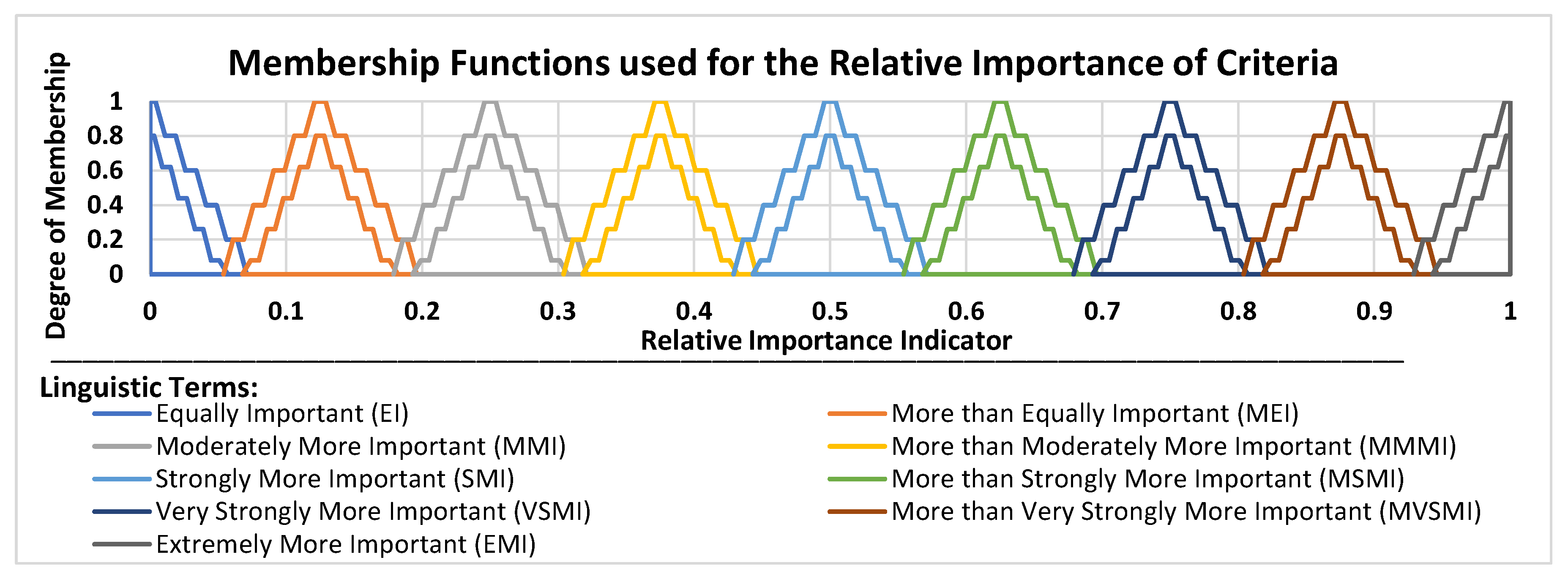
3.5. The Dynamic Icosagonal Fuzzy TOPSIS with Adaptive Criteria Weights

The Dynamic Icosagonal Fuzzy TOPSIS with Adaptive Criteria Weights (DIFT-ACW) algorithm improves the Icosagonal Fuzzy TOPSIS (IFT) methodology proposed in [40] by embedding the characteristics of the Dynamic Trapezoidal Fuzzy TOPSIS with Adaptive Criteria Weights (DTFT-ACW) algorithm described in [41]. Thus, the DIFT-ACW adapts its decisions according to specific factors such as the battery level of the user equipment. Regarding the implementations of the DIFT-ACW algorithm, suppose C = { C 1 , C 2 , , C m } is the set of criteria and w 1 , w 2 , , w m are the weights of each criterion. The criteria weights are adapted by taking into consideration the fact that some services could be more important than the others. In particular, the relative importance of each service q is determined using a priority vector Ω ˜ , which is calculated using Formula (14) where each ω i j ( t ) = [ ( ω i j 1 U ( t ) , ω i j 2 U ( t ) , ω i j 3 U ( t ) , ω i j 4 U ( t ) , ω i j 5 U ( t ) , ω i j 6 U ( t ) , ω i j 7 U ( t ) , ω i j 8 U ( t ) , ω i j 9 U ( t ) , ω i j 10 U ( t ) , ω i j 11 U ( t ) , ω i j 12 U ( t ) , ω i j 13 U ( t ) , ω i j 14 U ( t ) , ω i j 15 U ( t ) , ω i j 16 U ( t ) , ω i j 17 U ( t ) , ω i j 18 U ( t ) , ω i j 19 U ( t ) , ω i j 20 U ( t ) , v i j U ( t ) , v i j 1 U ( t ) , v i j 2 U ( t ) , v i j 3 U ( t ) , v i j 4 U ( t ) , v i j 5 U ( t ) , v i j 6 U ( t ) , v i j 7 U ( t ) , v i j 8 U ( t ) ) , ( ω i j 1 L ( t ) , ω i j 2 L ( t ) , ω i j 3 L ( t ) , ω i j 4 L ( t ) , ω i j 5 L ( t ) , ω i j 6 L ( t ) , ω i j 7 L ( t ) , ω i j 8 L ( t ) , ω i j 9 L ( t ) , ω i j 10 L ( t ) , ω i j 11 L ( t ) , ω i j 12 L ( t ) , ω i j 13 L ( t ) , ω i j 14 L ( t ) , ω i j 15 L ( t ) , ω i j 16 L ( t ) , ω i j 17 L ( t ) , ω i j 18 L ( t ) , ω i j 19 L ( t ) , ω i j 20 L ( t ) , v i j L ( t ) , v i j 1 L ( t ) , v i j 2 L ( t ) , v i j 3 L ( t ) , v i j 4 L ( t ) , v i j 5 L ( t ) , v i j 6 L ( t ) , v i j 7 L ( t ) , v i j 8 L ( t ) ) ] and Q is the number of the considered services.
Ω ˜ = [ ω ˜ 1 ω ˜ 2 ω ˜ Q ]
Furthermore, at each time t, a list A ( t ) = { A 1 ( t ) , A 2 ( t ) , , A z ( t ) } is constructed determining the current network alternatives.
In particular, initially, each x i j ( t ) element of the n × m decision matrix D ( t ) is an IVIFN, which expresses the performance of alternative i for the criterion j, as presented to Formula (25).
D ( t ) = C 1 ( t ) C m ( t ) A 1 ( t ) x 11 ( t ) x 1 m ( t ) A n ( t ) x n 1 ( t ) x n m ( t )
where: x i j ( t ) = [ ( x i j 1 U ( t ) , x i j 2 U ( t ) , x i j 3 U ( t ) , x i j 4 U ( t ) , x i j 5 U ( t ) , x i j 6 U ( t ) , x i j 7 U ( t ) , x i j 8 U ( t ) , x i j 9 U ( t ) , x i j 10 U ( t ) , x i j 11 U ( t ) , x i j 12 U ( t ) , x i j 13 U ( t ) , x i j 14 U ( t ) , x i j 15 U ( t ) , x i j 16 U ( t ) , x i j 17 U ( t ) , x i j 18 U ( t ) , x i j 19 U ( t ) , x i j 20 U ( t ) , v i j U ( t ) , v i j 1 U ( t ) , v i j 2 U ( t ) , v i j 3 U ( t ) , v i j 4 U ( t ) , v i j 5 U ( t ) , v i j 6 U ( t ) , v i j 7 U ( t ) , v i j 8 U ( t ) ) , ( x i j 1 L ( t ) , x i j 2 L ( t ) , x i j 3 L ( t ) , x i j 4 L ( t ) , x i j 5 L ( t ) , x i j 6 L ( t ) , x i j 7 L ( t ) , x i j 8 L ( t ) , x i j 9 L ( t ) , x i j 10 L ( t ) , x i j 11 L ( t ) , x i j 12 L ( t ) , x i j 13 L ( t ) , x i j 14 L ( t ) , x i j 15 L ( t ) , x i j 16 L ( t ) , x i j 17 L ( t ) , x i j 18 L ( t ) , x i j 19 L ( t ) , x i j 20 L ( t ) , v i j L ( t ) , v i j 1 L ( t ) , v i j 2 L ( t ) , v i j 3 L ( t ) , v i j 4 L ( t ) , v i j 5 L ( t ) , v i j 6 L ( t ) , v i j 7 L ( t ) , v i j 8 L ( t ) ) ] . In case there are Q services, the decision matrix includes the average of the performance values by applying Formula (26). Correspondingly, in this case, the criteria weights are obtained as the average of the individual weights of the considered services by applying Formula (27).
x i j ( t ) = 1 Q k = 1 Q x i j k ( t ) · ω k ( t )
w j ( t ) = 1 Q k = 1 Q w j k ( t )
Furthermore, for each network selection performed in time t, if D ( t ) = D ( t p r e v ) , then the ranks of the candidate networks obtained at time t p r e v are considered. Thus, the proposed algorithm achieves O ( n ) complexity in this case. Otherwise, the methods defined by the DIFT-ACW algorithm are performed. In this case, the algorithm achieves O ( n 2 ) complexity, which is also introduced by the most MADM methods proposed in the literature.
Thereafter, the decision matrix is normalized. To accomplish this task, the algorithm considers that Ω b is the set of benefit attributes and Ω c is the set of cost attributes. Subsequently, Formula (28) is applied for the estimation of the elements of the normalized decision matrix for the case of benefit attributes where b j ( t ) = max i x i j U ( t ) for each j Ω b . Correspondingly, Formula (29) is applied for the estimation of the elements of the normalized decision matrix for the case of cost attributes where c j ( t ) = min i x i j L ( t ) for each j Ω c .
r i j ( t ) = r i j ( t p r e v ) , if D ( t ) = D ( t p r e v ) [ ( x i j 1 U ( t ) b j ( t ) , x i j 2 U ( t ) b j ( t ) , x i j 3 U ( t ) b j ( t ) , x i j 4 U ( t ) b j ( t ) , x i j 5 U ( t ) b j ( t ) , x i j 6 U ( t ) b j ( t ) , x i j 7 U ( t ) b j ( t ) , x i j 8 U ( t ) b j ( t ) , x i j 9 U ( t ) b j ( t ) , x i j 10 U ( t ) b j ( t ) , x i j 11 U ( t ) b j ( t ) , x i j 12 U ( t ) b j ( t ) , x i j 13 U ( t ) b j ( t ) , x i j 14 U ( t ) b j ( t ) , x i j 15 U ( t ) b j ( t ) , x i j 16 U ( t ) b j ( t ) , x i j 17 U ( t ) b j ( t ) , x i j 18 U ( t ) b j ( t ) , x i j 19 U ( t ) b j ( t ) , x i j 20 U ( t ) b j ( t ) , v i j U ( t ) , v i j 1 U ( t ) , v i j 2 U ( t ) , v i j 3 U ( t ) , v i j 4 U ( t ) , v i j 5 U ( t ) , v i j 6 U ( t ) , v i j 7 U ( t ) , v i j 8 U ( t ) ) , ( x i j 1 L ( t ) b j ( t ) , x i j 2 L ( t ) b j ( t ) , x i j 3 L ( t ) b j ( t ) , x i j 4 L ( t ) b j ( t ) , x i j 5 L ( t ) b j ( t ) , x i j 6 L ( t ) b j ( t ) , x i j 7 L ( t ) b j ( t ) , x i j 8 L ( t ) b j ( t ) , x i j 9 L ( t ) b j ( t ) , x i j 10 L ( t ) b j ( t ) , x i j 11 L ( t ) b j ( t ) , x i j 12 L ( t ) b j ( t ) , x i j 13 L ( t ) b j ( t ) , x i j 14 L ( t ) b j ( t ) , x i j 15 L ( t ) b j ( t ) , x i j 16 L ( t ) b j ( t ) , x i j 17 L ( t ) b j ( t ) , x i j 18 L ( t ) b j ( t ) , x i j 19 L ( t ) b j ( t ) , x i j 20 L ( t ) b j ( t ) , v i j L ( t ) , v i j 1 L ( t ) , v i j 2 L ( t ) , v i j 3 L ( t ) , v i j 4 L ( t ) , v i j 5 L ( t ) , v i j 6 L ( t ) , v i j 7 L ( t ) , v i j 8 L ( t ) ) ] , if D ( t ) D ( t p r e v )
r i j ( t ) = r i j ( t p r e v ) , if D ( t ) = D ( t p r e v ) [ ( c j ( t ) x i j 1 U ( t ) , c j ( t ) x i j 2 U ( t ) , c j ( t ) x i j 3 U ( t ) , c j ( t ) x i j 4 U ( t ) , c j ( t ) x i j 5 U ( t ) , c j ( t ) x i j 6 U ( t ) , c j ( t ) x i j 7 U ( t ) , c j ( t ) x i j 8 U ( t ) , c j ( t ) x i j 9 U ( t ) , c j ( t ) x i j 10 U ( t ) , c j ( t ) x i j 11 U ( t ) , c j ( t ) x i j 12 U ( t ) , c j ( t ) x i j 13 U ( t ) , c j ( t ) x i j 14 U ( t ) , c j ( t ) x i j 15 U ( t ) , c j ( t ) x i j 16 U ( t ) , c j ( t ) x i j 17 U ( t ) , c j ( t ) x i j 18 U ( t ) , c j ( t ) x i j 19 U ( t ) , c j ( t ) x i j 20 U ( t ) , v i j U ( t ) , v i j 1 U ( t ) , v i j 2 U ( t ) v i j 3 U ( t ) , v i j 4 U ( t ) , v i j 5 U ( t ) , v i j 6 U ( t ) , v i j 7 U ( t ) , v i j 8 U ( t ) ) , ( c j ( t ) x i j 1 L ( t ) , c j ( t ) x i j 2 L ( t ) , c j ( t ) x i j 3 L ( t ) , c j ( t ) x i j 4 L ( t ) , c j ( t ) x i j 5 L ( t ) , c j ( t ) x i j 6 L ( t ) , c j ( t ) x i j 7 L ( t ) , c j ( t ) x i j 8 L ( t ) , c j ( t ) x i j 9 L ( t ) , c j ( t ) x i j 10 L ( t ) , c j ( t ) x i j 11 L ( t ) , c j ( t ) x i j 12 L ( t ) , c j ( t ) x i j 13 L ( t ) , c j ( t ) x i j 14 L ( t ) , c j ( t ) x i j 15 L ( t ) , c j ( t ) x i j 16 L ( t ) , c j ( t ) x i j 17 L ( t ) , c j ( t ) x i j 18 L ( t ) , c j ( t ) x i j 19 L ( t ) , c j ( t ) x i j 20 L ( t ) , v i j L ( t ) , v i j 1 L ( t ) , v i j 2 L ( t ) , v i j 3 L ( t ) , v i j 4 L ( t ) , v i j 5 L ( t ) , v i j 6 L ( t ) , v i j 7 L ( t ) , v i j 8 L ( t ) ) ] , if D ( t ) D ( t p r e v )
Subsequently, each element of the normalized decision matrix r i j ( t ) is multiplied with the respective weight w j ( t ) according to Formula (30) in order for the weighted normalized decision matrix to be created.
u i j ( t ) = u i j ( t p r e v ) , if D ( t ) = D ( t p r e v ) [ ( i j 1 U ( t ) · w j ( t ) , r i j 2 U ( t ) · w j ( t ) , r i j 3 U ( t ) · w j ( t ) , r i j 4 U ( t ) · w j ( t ) , r i j 5 U ( t ) · w j ( t ) , r i j 6 U ( t ) · w j ( t ) , r i j 7 U ( t ) · w j ( t ) , r i j 8 U ( t ) · w j ( t ) , r i j 9 U ( t ) · w j ( t ) , r i j 10 U ( t ) · w j ( t ) , r i j 11 U ( t ) · w j ( t ) , r i j 12 U ( t ) · w j ( t ) , r i j 13 U ( t ) · w j ( t ) , r i j 14 U ( t ) · w j ( t ) , r i j 15 U ( t ) · w j ( t ) , r i j 16 U ( t ) · w j ( t ) , r i j 17 U ( t ) · w j ( t ) , r i j 18 U ( t ) · w j ( t ) , r i j 19 U ( t ) · w j ( t ) , r i j 20 U ( t ) · w j ( t ) , v i j U ( t ) , v i j 1 U ( t ) , v i j 2 U ( t ) , v i j 3 U ( t ) , v i j 4 U ( t ) , v i j 5 U ( t ) , v i j 6 U ( t ) , v i j 7 U ( t ) , v i j 8 U ( t ) ) , ( r i j 1 L ( t ) · w j ( t ) , r i j 2 L ( t ) · w j ( t ) , r i j 3 L ( t ) · w j ( t ) , r i j 4 L ( t ) · w j ( t ) , r i j 5 L ( t ) · w j ( t ) , r i j 6 L ( t ) · w j ( t ) , r i j 7 L ( t ) · w j ( t ) , r i j 8 L ( t ) · w j ( t ) , r i j 9 L ( t ) · w j ( t ) , r i j 10 L ( t ) · w j ( t ) , r i j 11 L ( t ) · w j ( t ) , r i j 12 L ( t ) · w j ( t ) , r i j 13 L ( t ) · w j ( t ) , r i j 14 L ( t ) · w j ( t ) , r i j 15 L ( t ) · w j ( t ) , r i j 16 L ( t ) · w j ( t ) , r i j 17 L ( t ) · w j ( t ) , r i j 18 L ( t ) · w j ( t ) , r i j 19 L ( t ) · w j ( t ) , r i j 20 L ( t ) · w j ( t ) , v i j L ( t ) , v i j 1 L ( t ) , v i j 2 L ( t ) , v i j 3 L ( t ) , v i j 4 L ( t ) , v i j 5 L ( t ) , v i j 6 L ( t ) , v i j 7 L ( t ) , v i j 8 L ( t ) ) ] , if D ( t ) D ( t p r e v )
Then, the positive ideal solution is determined using Formula (31), where i max i if j Ω b and i min i if j Ω c .
X + ( t ) = X + ( t p r e v ) , if D ( t ) = D ( t p r e v ) [ ( i j 1 + U , x i j 2 + U ( t ) , x i j 3 + U ( t ) , x i j 4 + U ( t ) , x i j 5 + U ( t ) , x i j 6 + U ( t ) , x i j 7 + U ( t ) , x i j 8 + U ( t ) , x i j 9 + U ( t ) , x i j 10 + U ( t ) , x i j 11 + U ( t ) , x i j 12 + U ( t ) , x i j 13 + U ( t ) , x i j 14 + U ( t ) , x i j 15 + U ( t ) , x i j 16 + U ( t ) , x i j 17 + U ( t ) , x i j 18 + U ( t ) , x i j 19 + U ( t ) , x i j 20 + U ( t ) , v i j + U ( t ) , v i j 1 + U ( t ) , v i j 2 + U ( t ) , v i j 3 + U ( t ) , v i j 4 + U ( t ) , v i j 5 + U ( t ) , v i j 6 + U ( t ) , v i j 7 + U ( t ) , v i j 8 + U ) ( t ) , ( x i j 1 + L ( t ) , x i j 2 + L ( t ) , x i j 3 + L ( t ) , x i j 4 + L ( t ) , x i j 5 + L ( t ) , x i j 6 + L ( t ) , x i j 7 + L ( t ) , x i j 8 + L ( t ) , x i j 9 + L ( t ) , x i j 10 + L ( t ) , x i j 11 + L ( t ) , x i j 12 + L ( t ) , x i j 13 + L ( t ) , x i j 14 + L ( t ) , x i j 15 + L ( t ) , x i j 16 + L ( t ) , x i j 17 + L ( t ) , x i j 18 + L ( t ) , x i j 19 + L ( t ) , x i j 20 + L ( t ) , v i j + L ( t ) , v i j 1 + L ( t ) , v i j 2 + L ( t ) , v i j 3 + L ( t ) , v i j 4 + L ( t ) , v i j 5 + L ( t ) , v i j 6 + L ( t ) , v i j 7 + L ( t ) , v i j 8 + L ( t ) ) ] = i u i j 1 U ( t ) , i u i j 2 U ( t ) , i u i j 3 U ( t ) , i u i j 4 U ( t ) , i u i j 5 U ( t ) , i u i j 6 U ( t ) , i u i j 7 U ( t ) , i u i j 8 U ( t ) , i u i j 9 U ( t ) , i u i j 10 U ( t ) , i u i j 11 U ( t ) , i u i j 12 U ( t ) , i u i j 13 U ( t ) , i u i j 14 U ( t ) , i u i j 15 U ( t ) , i u i j 16 U ( t ) , i u i j 17 U ( t ) , i u i j 18 U ( t ) , i u i j 19 U ( t ) , i u i j 20 U ( t ) , v i j U ( t ) , v i j 1 U ( t ) , v i j 2 U ( t ) , v i j 3 U ( t ) , v i j 4 U ( t ) , v i j 5 U ( t ) , v i j 6 U ( t ) , v i j 7 U ( t ) , v i j 8 U ) ( t ) , ( i u i j 1 L ( t ) , i u i j 2 L ( t ) , i u i j 3 L ( t ) , i u i j 4 L ( t ) , i u i j 5 L ( t ) , i u i j 6 L ( t ) , i u i j 7 L ( t ) , i u i j 8 L ( t ) , i u i j 9 L ( t ) , i u i j 10 L ( t ) , i u i j 11 L ( t ) , i u i j 12 L ( t ) , i u i j 13 L ( t ) , i u i j 14 L ( t ) , i u i j 15 L ( t ) , i u i j 16 L ( t ) , i u i j 17 L ( t ) , i u i j 18 L ( t ) , i u i j 19 L ( t ) , i u i j 20 L ( t ) , v i j L ( t ) , v i j 1 L ( t ) , v i j 2 L ( t ) , v i j 3 L ( t ) , v i j 4 L ( t ) , v i j 5 L ( t ) , v i j 6 L ( t ) , v i j 7 L ( t ) , v i j 8 L ( t ) ) ] , if D ( t ) D ( t p r e v )
Similarly, the negative ideal solutions is calculated using Formula (32), where i min i if j Ω b and i max i if j Ω c .
X ( t ) = X ( t p r e v ) , if D ( t ) = D ( t p r e v ) [ ( i j 1 U ( t ) , x i j 2 U ( t ) , x i j 3 U ( t ) , x i j 4 U ( t ) , x i j 5 U ( t ) , x i j 6 U ( t ) , x i j 7 U ( t ) , x i j 8 U ( t ) , x i j 9 U ( t ) , x i j 10 U ( t ) , x i j 11 U ( t ) , x i j 12 U ( t ) , x i j 13 U ( t ) , x i j 14 U ( t ) , x i j 15 U ( t ) , x i j 16 U ( t ) , x i j 17 U ( t ) , x i j 18 U ( t ) , x i j 19 U ( t ) , x i j 20 U ( t ) , v i j U ( t ) , v i j 1 U ( t ) , v i j 2 U ( t ) , v i j 3 U ( t ) , v i j 4 U ( t ) , v i j 5 U ( t ) , v i j 6 U ( t ) , v i j 7 U ( t ) , v i j 8 U ) ( t ) , ( x i j 1 L ( t ) , x i j 2 L ( t ) , x i j 3 L ( t ) , x i j 4 L ( t ) , x i j 5 L ( t ) , x i j 6 L ( t ) , x i j 7 L ( t ) , x i j 8 L ( t ) , x i j 9 L ( t ) , x i j 10 L ( t ) , x i j 11 L ( t ) , x i j 12 L ( t ) , x i j 13 L ( t ) , x i j 14 L ( t ) , x i j 15 L ( t ) , x i j 16 L ( t ) , x i j 17 L ( t ) , x i j 18 L ( t ) , x i j 19 L ( t ) , x i j 20 L ( t ) , v i j L ( t ) , v i j 1 L ( t ) , v i j 2 L ( t ) , v i j 3 L ( t ) , v i j 4 L ( t ) , v i j 5 L ( t ) , v i j 6 L ( t ) , v i j 7 L ( t ) , v i j 8 L ( t ) ) ] = i u i j 1 U ( t ) , i u i j 2 U ( t ) , i u i j 3 U ( t ) , i u i j 4 U ( t ) , i u i j 5 U ( t ) , i u i j 6 U ( t ) , i u i j 7 U ( t ) , i u i j 8 U ( t ) , i u i j 9 U ( t ) , i u i j 10 U ( t ) , i u i j 11 U ( t ) , i u i j 12 U ( t ) , i u i j 13 U ( t ) , i u i j 14 U ( t ) , i u i j 15 U ( t ) , i u i j 16 U ( t ) , i u i j 17 U ( t ) , i u i j 18 U ( t ) , i u i j 19 U ( t ) , i u i j 20 U ( t ) , v i j U ( t ) , v i j 1 U ( t ) , v i j 2 U ( t ) , v i j 3 U ( t ) , v i j 4 U ( t ) , v i j 5 U ( t ) , v i j 6 U ( t ) , v i j 7 U ( t ) , v i j 8 U ) ( t ) , ( i u i j 1 L ( t ) , i u i j 2 L ( t ) , i u i j 3 L ( t ) , i u i j 4 L ( t ) , i u i j 5 L ( t ) , i u i j 6 L ( t ) , i u i j 7 L ( t ) , i u i j 8 L ( t ) , i u i j 9 L ( t ) , i u i j 10 L ( t ) , i u i j 11 L ( t ) , i u i j 12 L ( t ) , i u i j 13 L ( t ) , i u i j 14 L ( t ) , i u i j 15 L ( t ) , i u i j 16 L ( t ) , i u i j 17 L ( t ) , i u i j 18 L ( t ) , i u i j 19 L ( t ) , i u i j 20 L ( t ) , v i j L ( t ) , v i j 1 L ( t ) , v i j 2 L ( t ) , v i j 3 L ( t ) , v i j 4 L ( t ) , v i j 5 L ( t ) , v i j 6 L ( t ) , v i j 7 L ( t ) , v i j 8 L ( t ) ) ] , if D ( t ) D ( t p r e v )
Following this, Formulas (33) and (34) are applied in order for the distances of each candidate network from the positive ideal solution to be calculated. Similarly, (35) and (36) are applied in order for the distances of each candidate network from the negative ideal solution to be calculated.
d i 1 + ( t ) = d i 1 + ( t p r e v ) , if D ( t ) = D ( t p r e v ) j = 1 m { 1 20 [ ( u i j 1 U ( t ) x i j 1 + U ( t ) ) 2 + ( u i j 2 U ( t ) x i j 2 + U ( t ) ) 2 + ( u i j 3 U ( t ) x i j 3 + U ( t ) ) 2 + ( u i j 4 U ( t ) x i j 4 + U ( t ) ) 2 + ( u i j 5 U ( t ) x i j 5 + U ( t ) ) 2 + ( u i j 6 U ( t ) x i j 6 + U ( t ) ) 2 + ( u i j 7 U ( t ) x i j 7 + U ( t ) ) 2 + ( u i j 8 U ( t ) x i j 8 + U ( t ) ) 2 + ( u i j 9 U ( t ) x i j 9 + U ( t ) ) 2 + ( u i j 10 U ( t ) x i j 10 + U ( t ) ) 2 + ( u i j 11 U ( t ) x i j 11 + U ( t ) ) 2 + ( u i j 12 U ( t ) x i j 12 + U ( t ) ) 2 + ( u i j 13 U ( t ) x i j 13 + U ( t ) ) 2 + ( u i j 14 U ( t ) x i j 14 + U ( t ) ) 2 + ( u i j 15 U ( t ) x i j 15 + U ( t ) ) 2 + ( u i j 16 U ( t ) x i j 16 + U ( t ) ) 2 + ( u i j 17 U ( t ) x i j 17 + U ( t ) ) 2 + ( u i j 18 U ( t ) x i j 18 + U ( t ) ) 2 + ( u i j 19 U ( t ) x i j 19 + U ( t ) ) 2 + ( u i j 20 U ( t ) x i j 20 + U ( t ) ) 2 ] } 1 2 , if D ( t ) D ( t p r e v )
d i 2 + ( t ) = d i 2 + ( t p r e v ) , if D ( t ) = D ( t p r e v ) j = 1 m { 1 20 [ ( u i j 1 L ( t ) x i j 1 + L ( t ) ) 2 + ( u i j 2 L ( t ) x i j 2 + L ( t ) ) 2 + ( u i j 3 L ( t ) x i j 3 + L ( t ) ) 2 + ( u i j 4 L ( t ) x i j 4 + L ( t ) ) 2 + ( u i j 5 L ( t ) x i j 5 + L ( t ) ) 2 + ( u i j 6 L ( t ) x i j 6 + L ( t ) ) 2 + ( u i j 7 L ( t ) x i j 7 + L ( t ) ) 2 + ( u i j 8 L ( t ) x i j 8 + L ( t ) ) 2 + ( u i j 9 L ( t ) x i j 9 + L ( t ) ) 2 + ( u i j 10 L ( t ) x i j 10 + L ( t ) ) 2 + ( u i j 11 L ( t ) x i j 11 + L ( t ) ) 2 + ( u i j 12 L ( t ) x i j 12 + L ( t ) ) 2 + ( u i j 13 L ( t ) x i j 13 + L ( t ) ) 2 + ( u i j 14 L ( t ) x i j 14 + L ( t ) ) 2 + ( u i j 15 L ( t ) x i j 15 + L ( t ) ) 2 + ( u i j 16 L ( t ) x i j 16 + L ( t ) ) 2 + ( u i j 17 L ( t ) x i j 17 + L ( t ) ) 2 + ( u i j 18 L ( t ) x i j 18 + L ( t ) ) 2 + ( u i j 19 L ( t ) x i j 19 + L ( t ) ) 2 + ( u i j 20 L ( t ) x i j 20 + L ( t ) ) 2 ] } 1 2 , if D ( t ) D ( t p r e v )
d i 1 ( t ) = d i 1 ( t p r e v ) , if D ( t ) = D ( t p r e v ) j = 1 m { 1 20 [ ( u i j 1 U ( t ) x i j 1 U ( t ) ) 2 + ( u i j 2 U ( t ) x i j 2 U ( t ) ) 2 + ( u i j 3 U ( t ) x i j 3 U ( t ) ) 2 + ( u i j 4 U ( t ) x i j 4 U ( t ) ) 2 + ( u i j 5 U ( t ) x i j 5 U ( t ) ) 2 + ( u i j 6 U ( t ) x i j 6 U ( t ) ) 2 + ( u i j 7 U ( t ) x i j 7 U ( t ) ) 2 + ( u i j 8 U ( t ) x i j 8 U ( t ) ) 2 + ( u i j 9 U ( t ) x i j 9 U ( t ) ) 2 + ( u i j 10 U ( t ) x i j 10 U ( t ) ) 2 + ( u i j 11 U ( t ) x i j 11 U ( t ) ) 2 + ( u i j 12 U ( t ) x i j 12 U ( t ) ) 2 + ( u i j 13 U ( t ) x i j 13 U ( t ) ) 2 + ( u i j 14 U ( t ) x i j 14 U ( t ) ) 2 + ( u i j 15 U ( t ) x i j 15 U ( t ) ) 2 + ( u i j 16 U ( t ) x i j 16 U ( t ) ) 2 + ( u i j 17 U ( t ) x i j 17 U ( t ) ) 2 + ( u i j 18 U ( t ) x i j 18 U ( t ) ) 2 + ( u i j 19 U ( t ) x i j 19 U ( t ) ) 2 + ( u i j 20 U ( t ) x i j 20 U ( t ) ) 2 ] } 1 2 , if D ( t ) D ( t p r e v )
d i 2 ( t ) = d i 2 ( t p r e v ) , if D ( t ) = D ( t p r e v ) j = 1 m { 1 20 [ ( u i j 1 L ( t ) x i j 1 L ( t ) ) 2 + ( u i j 2 L ( t ) x i j 2 L ( t ) ) 2 + ( u i j 3 L ( t ) x i j 3 L ( t ) ) 2 + ( u i j 4 L ( t ) x i j 4 L ( t ) ) 2 + ( u i j 5 L ( t ) x i j 5 L ( t ) ) 2 + ( u i j 6 L ( t ) x i j 6 L ( t ) ) 2 + ( u i j 7 L ( t ) x i j 7 L ( t ) ) 2 + ( u i j 8 L ( t ) x i j 8 L ( t ) ) 2 + ( u i j 9 L ( t ) x i j 9 L ( t ) ) 2 + ( u i j 10 L ( t ) x i j 10 L ( t ) ) 2 + ( u i j 11 L ( t ) x i j 11 L ( t ) ) 2 + ( u i j 12 L ( t ) x i j 12 L ( t ) ) 2 + ( u i j 13 L ( t ) x i j 13 L ( t ) ) 2 + ( u i j 14 L ( t ) x i j 14 L ( t ) ) 2 + ( u i j 15 L ( t ) x i j 15 L ( t ) ) 2 + ( u i j 16 L ( t ) x i j 16 L ( t ) ) 2 + ( u i j 17 L ( t ) x i j 17 L ( t ) ) 2 + ( u i j 18 L ( t ) x i j 18 L ( t ) ) 2 + ( u i j 19 L ( t ) x i j 19 L ( t ) ) 2 + ( u i j 20 L ( t ) x i j 20 L ( t ) ) 2 ] } 1 2 , if D ( t ) D ( t p r e v )
Thereafter, in a way similar to [37], the distances of the candidate networks from the positive and negative ideal solutions are expressed using intervals such as [ d i 1 + , d i 2 + ] and [ d i 1 , d i 2 ] . Finally, the relative closeness of the distances from the ideal solutions are computed using Formulas (37) and (38).
R C i 1 ( t ) = R C i 1 ( t p r e v ) , if D ( t ) = D ( t p r e v ) d i 1 ( t ) d i 1 + ( t ) + d i 1 ( t ) , if D ( t ) D ( t p r e v )
and:
R C i 2 ( t ) = R C i 2 ( t p r e v ) , if D ( t ) = D ( t p r e v ) d i 2 ( t ) d i 2 + ( t ) + d i 2 ( t ) , if D ( t ) D ( t p r e v )
The compound relative closeness is obtained by calculating the average of the R C i 1 ( t ) and R C i 2 ( t ) values using Formula (39).
R C i ( t ) = R C i ( t p r e v ) , if D ( t ) = D ( t p r e v ) R C i 1 ( t ) + R C i 2 ( t ) 2 , if D ( t ) D ( t p r e v )
The candidate networks are ranked by taking into consideration their R C i values, and the one with the higher R C i value is considered as the best alternative.

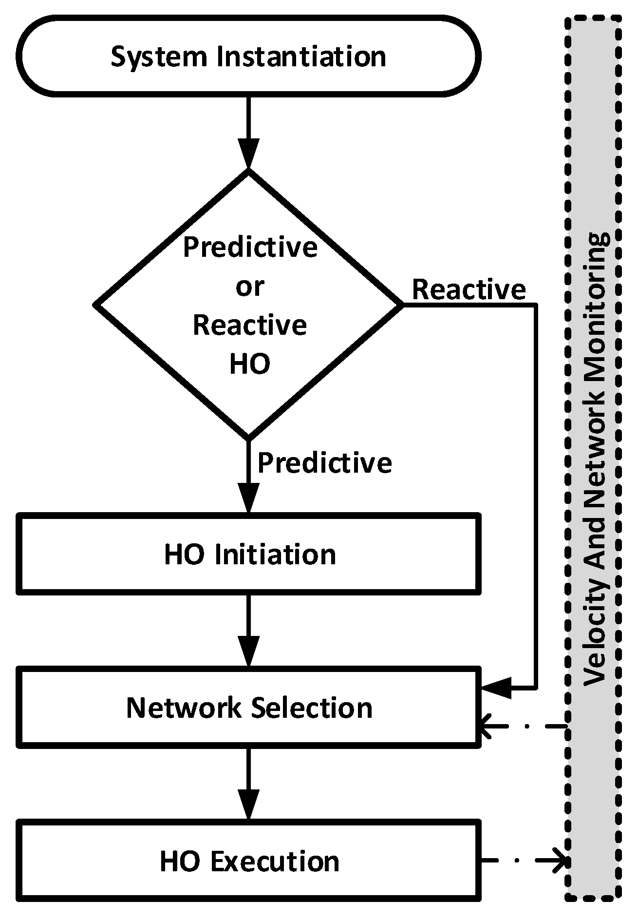
4. The Proposed Mobility Management Scheme

During vehicles’ movement, the velocity and network monitoring process is executed, enabling the effective transmission of each vehicle to the target access network in the case of an HO event. The HO process includes the HO initiation, the network selection, and the HO execution procedures, while both predictive and reactive HO operations are supported. In the case of predictive HO, HO initiation, network selection, and HO execution are performed, while in the case of reactive HO, the HO initiation is not performed since the link between the vehicle and its previous serving network goes down unexpectedly without an indication of a potential connection loss. Figure 3 presents the workflow of the proposed methodology. The design of the discussed scheme was optimized to be applied in 5G network architectures where both Fog and Cloud infrastructures are available, while the implemented signaling combines messages of both the IEEE 802.21 Media Independent Handover (MIH) [42] and the IETF Proxy Mobile IPv6 (PMIPv6) [43] standards. Furthermore, it should be noted that the proposed scheme can be used for the mobility management of both pedestrian and vehicular users. More specifically, handling the mobility issues in dynamic vehicular environments is of paramount importance, since the vehicles may move with increased velocities and provide heterogeneous services to multiple onboard users. Thus, this paper proposes and evaluates an HO scheme that can be adopted in a challenging vehicular network.

4.1. Velocity and Alternative Network Monitoring
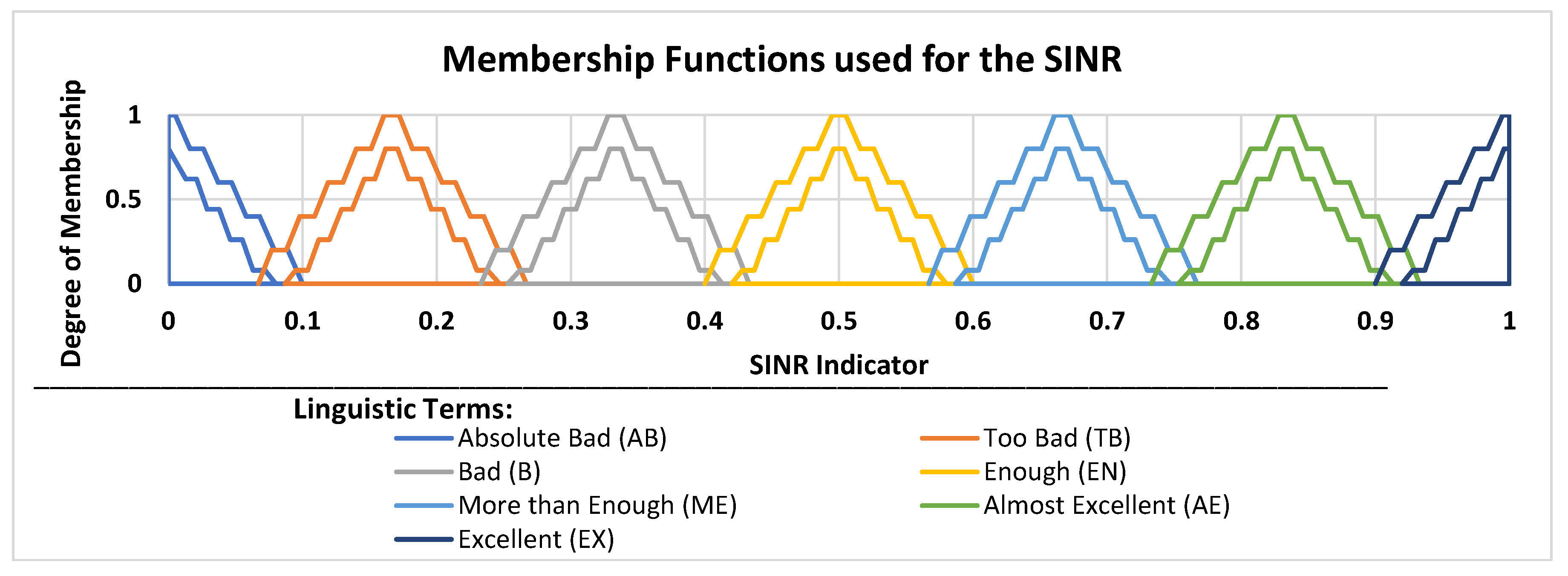
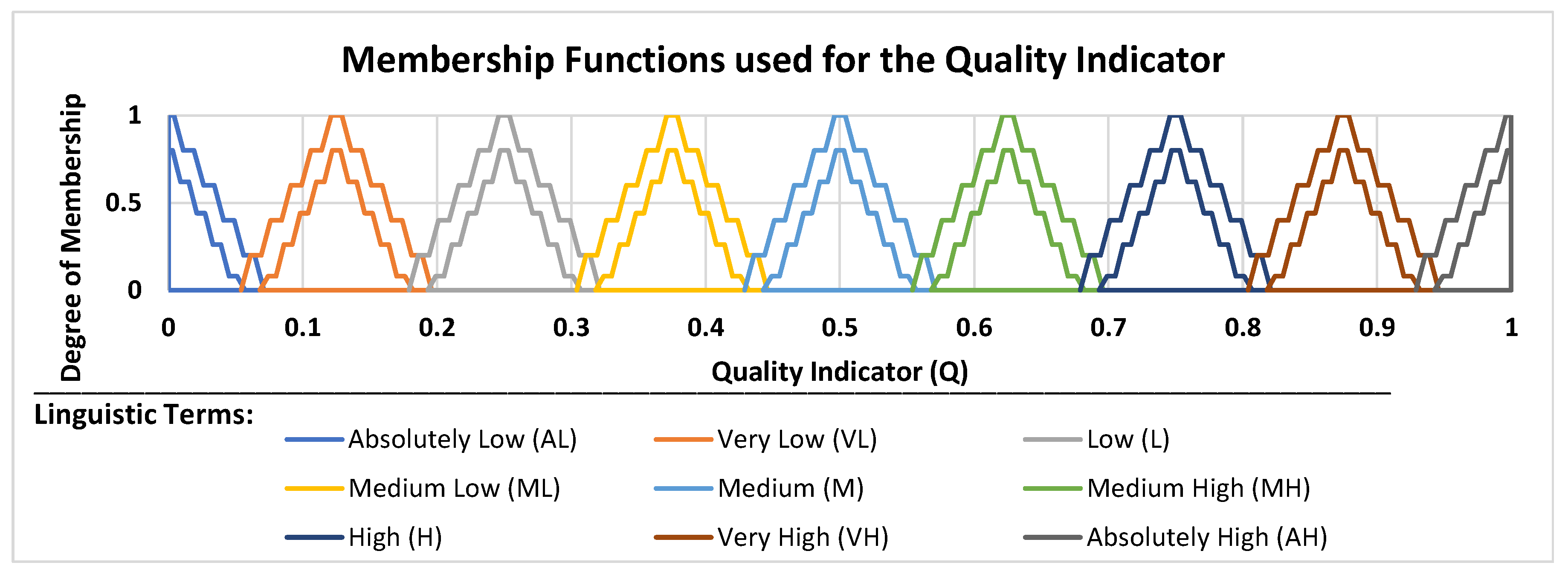
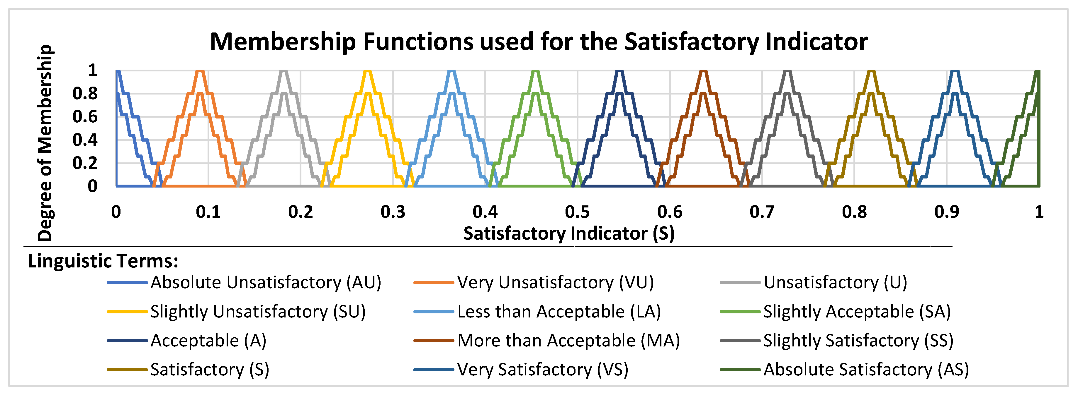
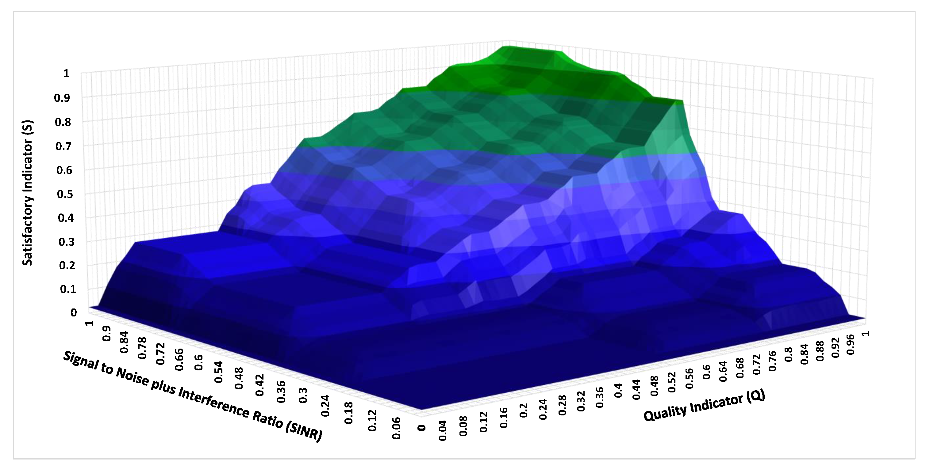
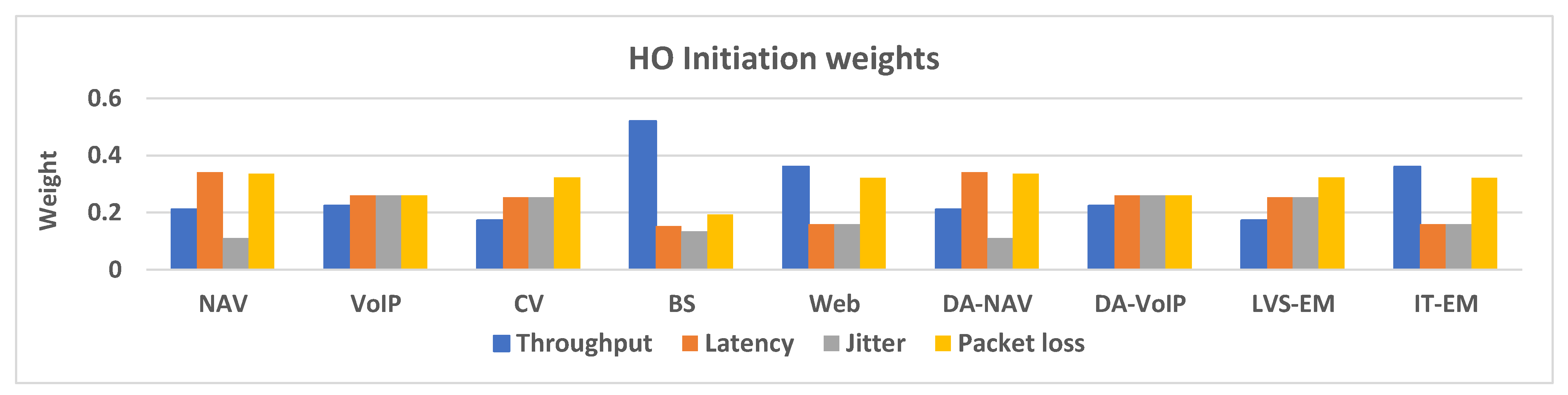
The Cloud/Fog infrastructure continuously monitors the velocity of each vehicle by applying the methodology described in [23]. Specifically, an improved version of the Mobility State Estimation (MSE) technique defined in 3GPP LTE Release 11 [22] was applied. This methodology categorizes the moving velocity of the vehicle as Normal, Medium, or High, by taking into consideration the number of HOs N C R u that the vehicle has performed during a sliding time window T C R m a x .
Additionally, each vehicle maintains a set A = { A 1 , A 2 , , A n } of candidate networks based on the SINR perceived from each one of them as specified by the Cloud/Fog environment. The set A is continuously updated, since the SINR of each network is constantly changing as the vehicle moves inside the wireless network access environment. Thereafter, in the case of predictive HO, the HO initiation will be performed, while in the case of reactive HO, the network selection is immediately executed.

4.2. HO Initiation

HO initiation is performed only in the case of predictive HO. During the HO initiation, the methodology described in [23] is applied. Specifically, the S u , i indicator is defined, determining the satisfaction grade of user u from his/her current network i. The value of the S u , i indicator is calculated using the MIFIS algorithm where the normalized values of the SINR and the QoS the vehicle perceives from its current network are used as the inputs. In this work, the MIFIS was implemented using the IVIFNs presented in Figure 4, Figure 5 and Figure 6.
During the instantiation of the system, the Satisfaction Indicators Chart (SIC) presented in Figure 7 is created at the Fog by applying the knowledge base described in [44]. The SIC chart presents the S u , i values obtained for each possible SINR and QoS combination. When either the SINR or the QoS drops below a predefined threshold, the vehicle sends the obtained values to the MAG of its current network using an M I H _ L i n k _ G o i n g _ d o w n [45] message. Subsequently, the Fog infrastructure where the current MAG belongs uses the SIC chart, in order for the S u , i satisfaction grade of the user to be determined. Subsequently, the network selection process will be performed if the estimated satisfaction grade is less than a predefined S t h threshold value.

4.3. Network Selection

During the network selection (Figure 8), the vehicle sends a 1 . M I H _ G e t _ I n f o r m a t i o n _ - R e q u e s t to the MIIS. This message embeds information about the services and the remaining energy of the vehicle. In the case of predictive HO, the message is transmitted by the current network of the vehicle. However, in the case of reactive HO, the vehicle chooses the network alternative with the higher SINR to transmit the message, since the connection with the current network has been lost. Subsequently, the velocity and network monitoring process considers the mobility state of each vehicle to create a subset A A of the available networks. Specifically, if the vehicle’s velocity has been characterized as Normal, then all the available networks are considered as alternatives, including both Macrocells and Femtocells in the A subset. On the other hand, if the vehicle’s velocity has been characterized as Medium, then some Femtocells are skipped along the vehicle’s trajectory and are not included in A . In particular, the Femtocell i is considered as an alternative if the estimated residence time of the vehicle u ( t u , i r e s i d e n c e ) is greater than or equal to the average residence time of the vehicle considering all the available Femtocells in its current location. It has to be noted that the t u , i r e s i d e n c e parameter of vehicle u for the ith cell is estimated using Formula (40) [46], where r f is the cell radius and v u is the vehicle velocity obtained by Formula (41) [47]. The λ u parameter represents the cell’s density in the location of the vehicle, as it is obtained by the Software-Defined Networking (SDN) controller. Finally, if vehicle’s velocity has been characterized as High, then only the available Macrocells are included in the A as alternatives.
t u , i r e s i d e n c e = π · r i 2 · v u
v u = π · N C R u 4 · T C R m a x · λ u
Following this, the availability of the resources offered from each network of the subset A is considered, so that a subset A A is created. Specifically, the MIIS checks the availability of the resources offered from each network alternative by exchanging 2 . M I H _ N 2 N _ H O _ Q u e r y _ R e s o u r c e _ R e q u e s t and 3 . M I H _ N 2 N _ H O _ Q u e r y _ R e s o u r c e _ R e - s p o n s e messages. Thereafter, networks included in the subset A” are ranked using the DIFT-ACW algorithm. The ranking is performed considering both network characteristics (throughput, latency, jitter, packet loss, and energy consumption) and the operator’s policy criteria (service reliability, security, and monetary cost) that each network offers for the services of the vehicle. Since the energy consumption parameter is considered during the ranking process, energy-intensive networks such as LTE-A Pro FD-MIMO, which operates with multiple antennas, obtain a low score for vehicles with low remaining energy of the user equipment. Furthermore, since the decision is made considering the vehicle’s velocity, as well as QoS and policy-related parameters, the ping-pong HO effect is eliminated. Following this, the network that obtains the higher score is selected, while the vehicle is informed about the target access network through a 4 . M I H _ G e t _ I n f o r m a t i o n _ R e s p o n s e message.

4.4. HO Execution

An improved scheme for the HO execution is proposed based on the FPMIPv6 protocol. Furthermore, if the selected and the current network belong to different MAGs, inter-MAG HO execution is performed. On the contrary, if the two networks belong to the same MAG, intra-MAG HO execution is performed.

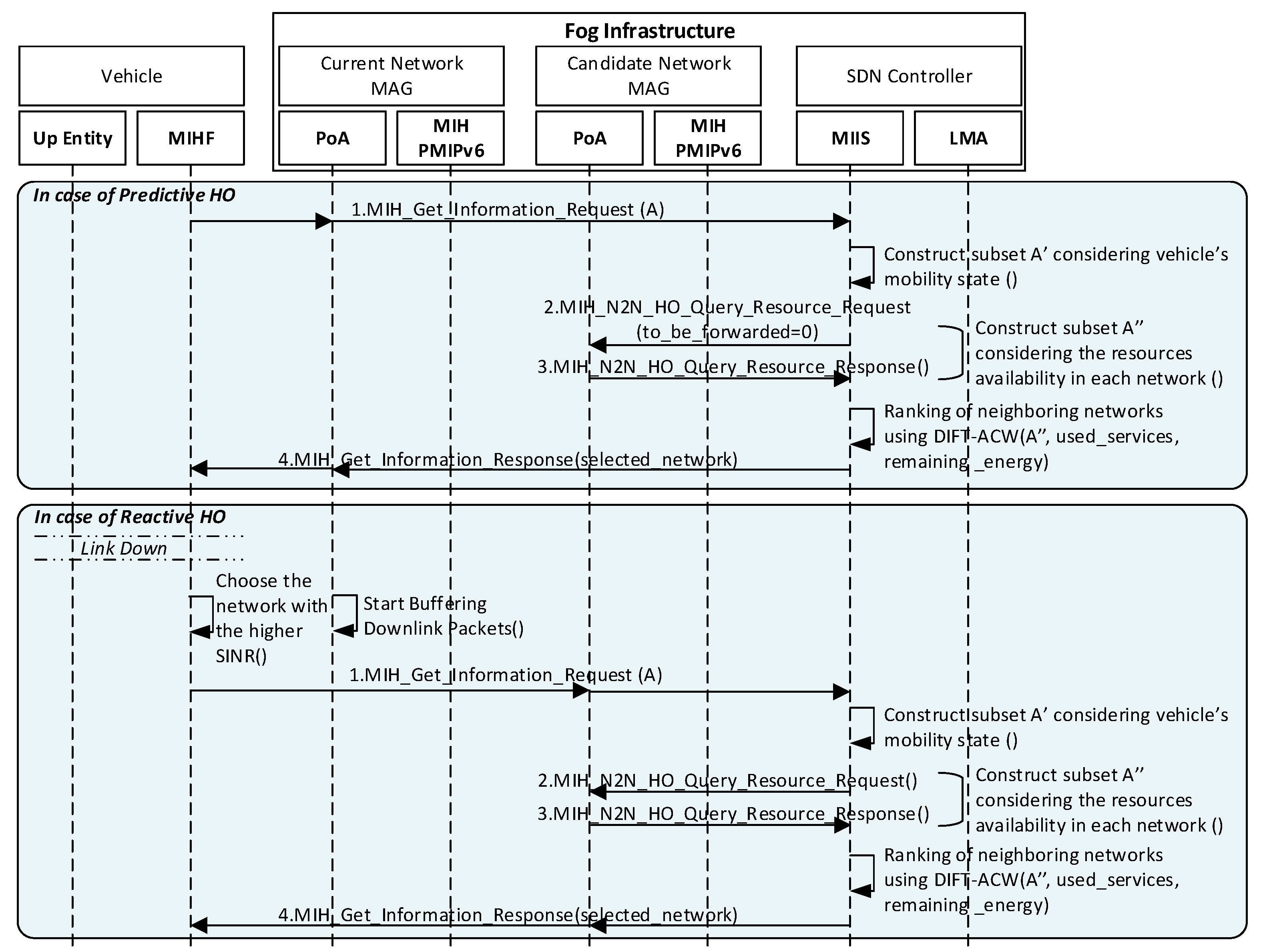
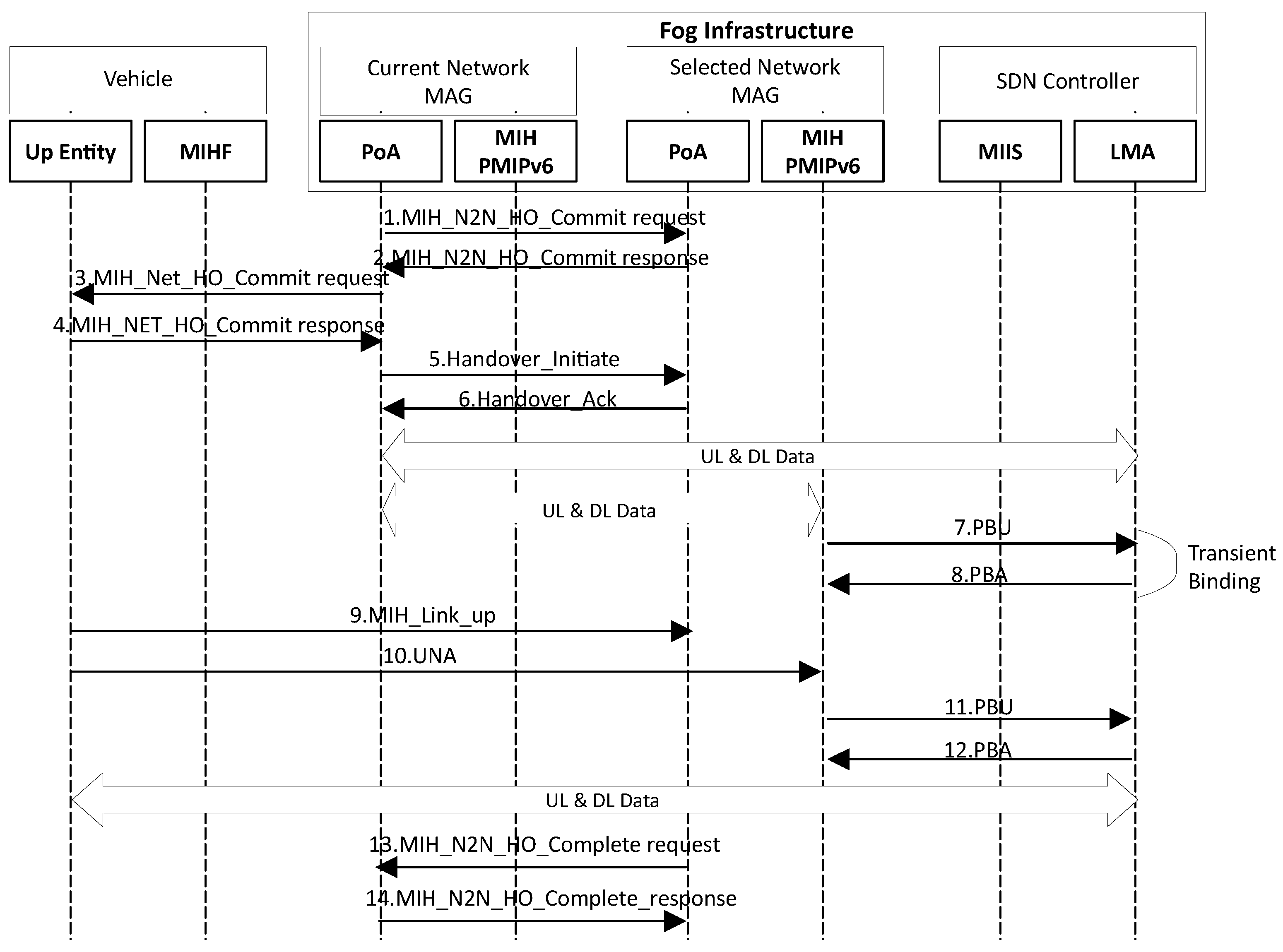
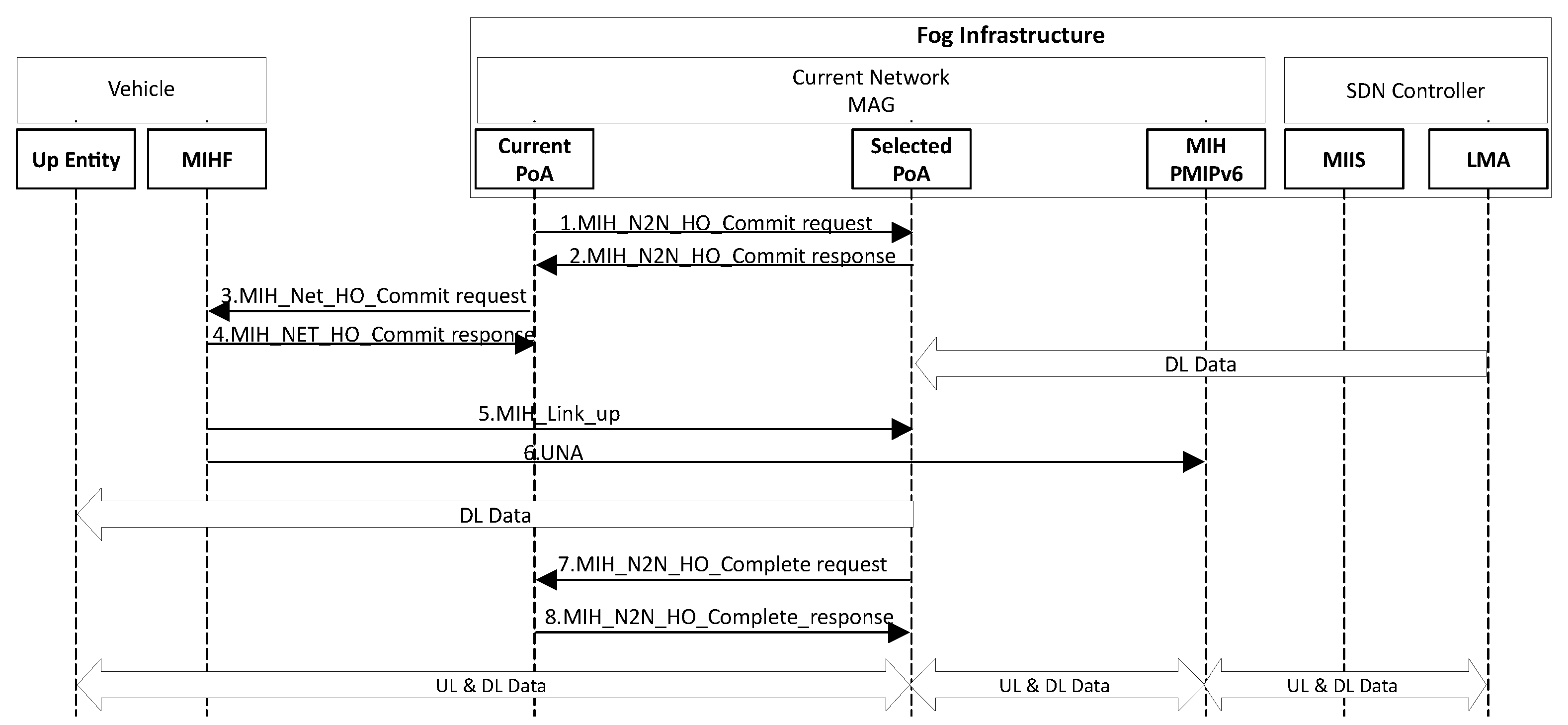
4.4.1. Proposed Predictive HO Scheme

In the case of predictive inter-MAG HO execution (Figure 9), the current network initially sends a 1 . M I H _ N 2 N _ H O _ C o m m i t _ r e q u e s t to the selected MAG to reserve the necessary resources for the upcoming handover. Following this, the selected MAG responds with a 2 . M I H _ N 2 N _ H O _ C o m m i t _ r e s p o n s e message indicating that the required resources have been reserved. In this case, the current MAG informs the vehicle about the successful resource allocation at the selected network using a 3 . M I H _ N e t _ H O _ C o m m i t _ r e q u e s t message, while the vehicle acknowledges the reception of the information using a 4 . M I H _ N e t _ - H O _ C o m m i t _ r e s p o n s e message.
Subsequently, the MAG of the current network sends a 5 . H a n d o v e r _ I n i t i a t e message to the MAG of the selected one, which includes the MN Identifier (MN-ID), the Home Network Prefix (HNP), and the MN Logical Link Identifier (MN-LLID). Furthermore, the Proxy (P) and the Buffering (B) flags of the message are set equal to 1 to inform the selected MAG that the buffering of data has been performed at the current MAG. By receiving this message, the MAG of the selected network replies with a 6 . H a n d o v e r _ A c k message, which acknowledges that the aforementioned information has been successfully received, while a bi-directional tunnel is established between the two MAGs. Thereafter, a copy of the buffered packets from the current MAG is transmitted through the tunnel to the selected MAG to be delivered to the vehicle when it connects to the selected network. Subsequently, the new MAG sends a 7 . P B U message to the LMA to create a transient record in the binding cache. Once the temporal binding is established at the LMA, it sends a 8 . P B A message to the MAG of the selected network, and a bi-directional tunnel is established between the two entities. Thus, downlink packets are forwarded from the LMA to the MAG of the selected network where they are buffered to be delivered to the vehicle when it completes its HO to the selected network. Furthermore, the bi-directional tunnel between the current MAG and the LMA remains active until the transient binding becomes permanent. Then, the transient binding introduces a smooth way for performing the handover by gradually changing the current MAG to avoid packet losses and false HOs.
Subsequently, the vehicle sends a 9 . M I H _ L i n k _ u p message to the selected MAG to enable the communication channel. Furthermore, the vehicle sends a 10 . U N A message to the selected network, to complete the establishment of both the Link and Network layers. Thereafter, the MAG of the selected network exchanges the 11 . P B U and 12 . P B A messages with the LMA to finalize the binding. Finally, the selected network sends a 13 . M I H _ N 2 N _ C o m p l e t e _ r e q u e s t message to the previous network. By receiving this message, the previous network releases the resources that have been reserved for the vehicle and sends back a 14 . M I H _ N 2 N _ C o m p l e t e _ r e s p o n s e message to finalize the HO execution.
Similar to the predictive inter-MAG HO execution, in the case of the predictive intra-MAG HO execution (Figure 10), the current network sends a 1 . M I H _ N 2 N _ H O _ C o m m i t _ r e q u e s t to the selected network to reserve the necessary resources for the upcoming handover. Following this, the selected network responds with a 2 . M I H _ N 2 N _ H O _ C o m m i t _ r e s p o n s e message indicating that the required resources have been reserved. In this case, the current network informs the vehicle about the successful resource allocation at the selected network using a 3 . M I H _ N e t _ H O _ C o m m i t _ r e q u e s t message, while the vehicle acknowledges the reception of the information using a 4 . M I H _ N e t _ H O _ C o m m i t _ r e s p o n s e message. Subsequently, the vehicle sends a 5 . M I H _ L i n k _ u p message to the selected network to enable the communication channel. Furthermore, the vehicle sends a 6 . U N A message to the selected network, to complete the establishment of both the Link and Network layers. Finally, the selected network replies back with a 7 . M I H _ N 2 N _ C o m p l e t e _ r e q u e s t to the current one. By receiving this message, the MAG releases the resources that have been reserved for the current network and replies back with a 8 . M I H _ N 2 N _ C o m p l e t e _ r e s p o n s e message to successfully finish the HO execution.
It has to be noted that in the case of predictive intra-MAG HO execution (Figure 10), since the involved networks are served by the same MAG, the use of 5 . H a n d o v e r _ I n i t i a t e and 6 . H a n d o v e r _ A c k messages is not necessary [48], as the MN-ID, the MN-LLID, and the Local Mobility Anchor Address (LMAA) are already known by their common MAG. Furthermore, the MAG does not exchange 7 . P B U and 8 . P B A messages with the LMA since it retains a Proxy Binding Update List (PBUL). Specifically, the MAG’s PB-UL stores information about the vehicle including the MN-ID, the Mobile Network Prefix (MNP), and the vehicle’s current network. Thus, when the vehicle performs an intra-MAG handover, the MNP is obtained from the PBUL. Furthermore, due to the common serving MAG, false handovers do not cause any malfunction.

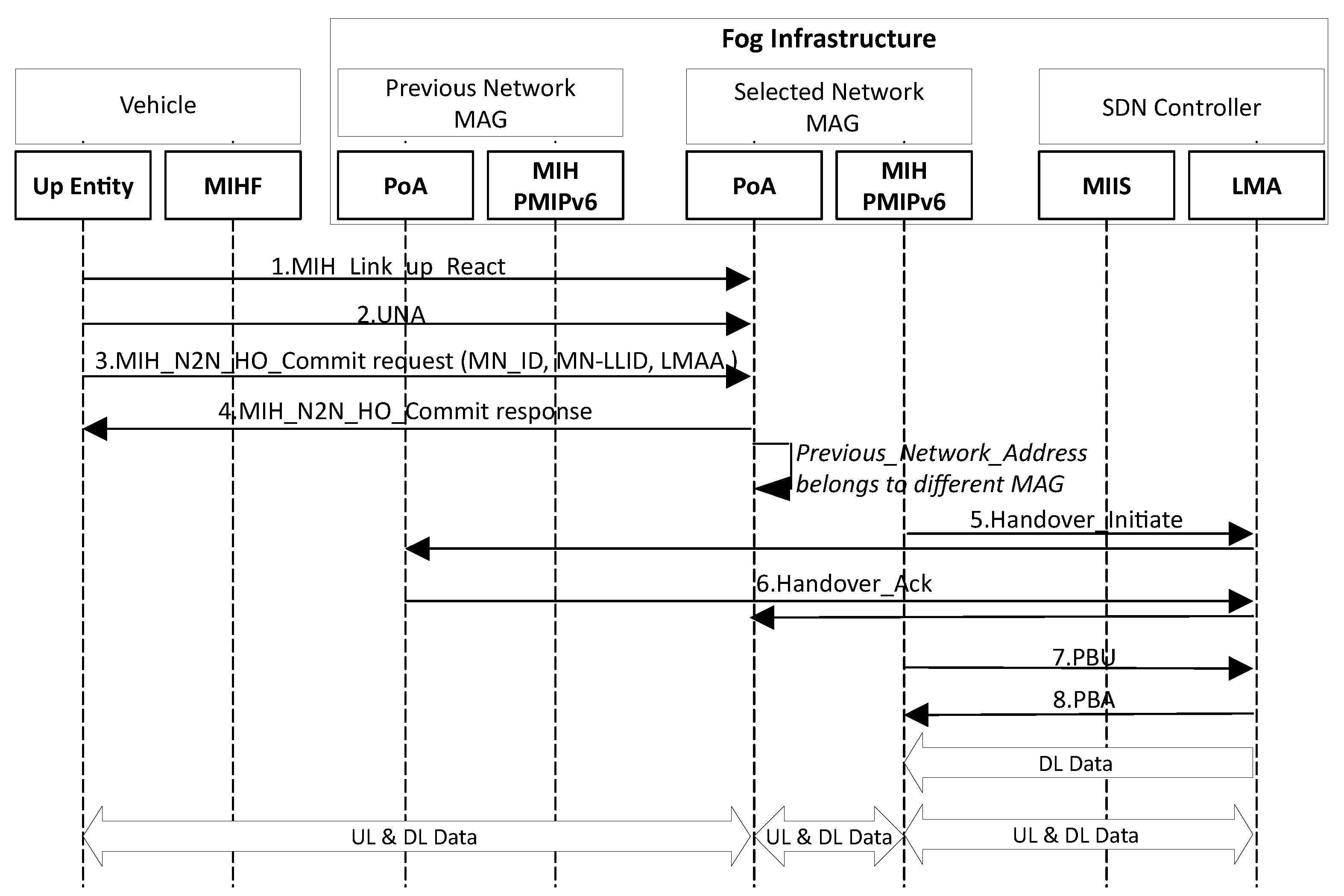
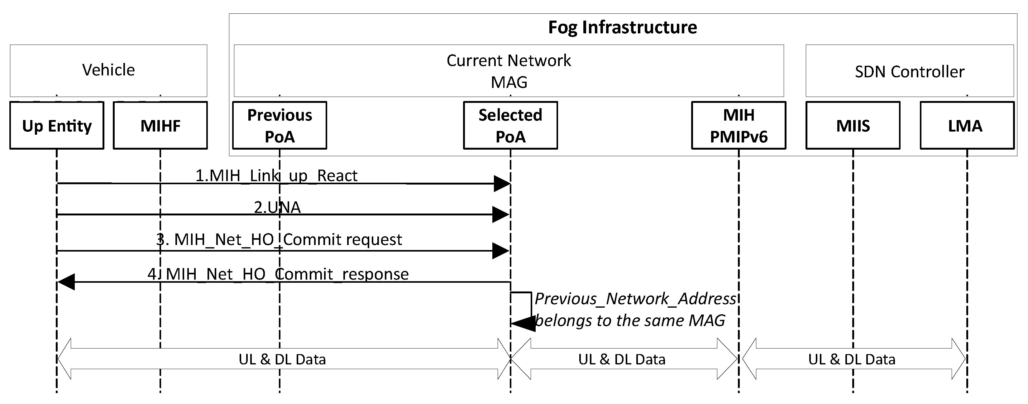
4.4.2. Proposed Reactive HO Scheme

In the case of reactive inter-MAG HO execution (Figure 11), the vehicle sends a 1 . M I H _ L i - n k _ u p _ R e a c t to the selected network, which includes information about the MN-ID and the MN-LLID and enables the communication channel. Subsequently, the vehicle sends a 2 . U N A message to the selected network, to complete the establishment of both the Link and Network layers, as well as a 3 . M I H _ N 2 N _ H O _ C o m m i t _ r e q u e s t message to reserve the required resources. By receiving this message, the selected network reserves the required resources and sends back a 4 . M I H _ N 2 N _ H O _ C o m m i t _ r e s p o n s e to the vehicle.
Thereafter, the MAG of the selected network identifies that the vehicle was not previously connected to any of the networks that it manipulates. Thus, the selected network sends a 5 . H a n d o v e r _ I n i t i a t e message to the previous one through the LMA. In this message, the Proxy (P) and the Buffering (B) flags of the message are set equal to 1. By receiving this message, the previous network responds with a 6 . H a n d o v e r _ A c k message, and a bi-directional tunnel is established between the two networks. Thereafter, the buffered packets from the previous network are transmitted through the tunnel to the selected network to be delivered to the vehicle when its HO completes. Furthermore, the MAG of the selected network exchanges the 7 . P B U and 8 . P B A messages with the LMA to update the Binding Cache Entry (BCE) of the LMA. Consequently, the vehicle becomes ready to transmit or receive packets through the selected network.
For the intra-MAG reactive VHO execution (Figure 12), the messages after the 4 . M I H _ - N 2 N _ H O _ C o m m i t _ r e s p o n s e of the above case are not exchanged between the vehicle and the selected network. Specifically, in this case, the MAG of the selected network identifies that the vehicle was previously connected to a network that it manipulates. Thus, the exchange of signaling messages between the MAG and the LMA is not required, and the vehicle is ready to transmit or receive packets through the selected network.
Finally, it has to be noted that after the successful execution of each of the above HO schemes, the number of handovers for the vehicle N C R u is increased for the estimation of the vehicle’s velocity.

4.5. The Computational Complexity of the Proposed Scheme

As far as the computational complexity of the proposed methodology is concerned, the worst-case scenario is observed during the network selection process. In particular, during the first run of the DIFT-ACW algorithm, an O ( n 2 ) complexity is introduced due to the weighting and the normalization of the two-dimensional decision matrices. Nevertheless, a constant time duration is required for the algorithm execution provided that D ( t ) = D ( t p r e v ) . In this case, the algorithm checks only the recent results obtained during the time period t p r e v , and an O ( n ) complexity is observed.

5. Simulation Setup and Results

In our simulation, the software-defined vehicular cloud topology presented in Figure 13 was evaluated. A mobility trace designating the map of the city of Athens along with transportation data was generated using the Open Street Map (OSM) software. Afterwards, the mobility trace was used as the input in the Simulator of Urban Mobility (SUMO), establishing a realistic mobility pattern including 77,797 vehicles driving inside Athens within a 24 h period of time. The network topology, as well as a Cloud/Fog infrastructure were created on the map using Network Simulator 3 (NS3) [49].
The Fog infrastructure consists of 28 802.11p WAVE RSUs, 5 LTE-A Pro FD-MIMO Macrocell e-Node Bs (eNBs), 8 LTE-A Macrocell eNBs, 70 LTE-A Femtocells eNBs, 8 WiMAX Macrocell Base Stations (BSs), and 41 WiMAX Femtocell BSs, equipped with additional computational and storage resources. Furthermore, the access networks are located in geographical positions based on the data available from the Hellenic Telecommunications and Post Commission (EETT) [50]. The positions and the spectrum of the base stations are presented in Table A2, Table A3, Table A4 (Appendix A) for the LTE-A Pro, the LTE-A, as well as the WiMAX and the WAVE technologies, respectively. Furthermore, the Fog infrastructure includes an SDN controller that constantly monitors the entire topology by implementing the Mobility Management as a Service (MMaS) model. Additional components including the Fog Manager, Fog Monitor, Network Manager, Network Monitor, Topology Discovery, Joint Resource Provisioner, and Power Consumption Estimator are incorporated into the Fog and are administered by the SDN controller. Specifically, the Fog Manager, as well as the Fog Monitor control the available resources of the topology. At the same time, the Network Manager manipulates OpenFlow forwarding tables, default path settings, and QoS-aware configurations. The Network Monitor provides the status of the switches of the entire infrastructure. Furthermore, the Topology Discovery component stores information about the generated topologies and the available UEs. Moreover, the Joint Resource Provisioner is utilized as a load coordinator for the VMs, the nodes, and the network traffic. Finally, the Power Consumption Estimator identifies the energy-demanding network access elements.
The Cloud infrastructure deploys a number of Virtual Machines (VMs) providing both Non-Disaster Management (nDM) and Disaster Management (DM) services. In particular, the nDM services include Navigation Assistance (NAV), Voice over IP (VoIP), Conversational Video (CV), Buffered Streaming (BS), and Web Browsing (Web) applications. On the other hand, DM services include Disaster-Aware Navigation Assistance (DA-NAV), Disaster-Aware Voice over IP (DA-VoIP), Live Video Streaming for Emergency Manipulation (LVS-EM), and Image Transmission for Emergency Manipulation (IT-EM) systems. Furthermore, the Cloud infrastructure includes a Software-Defined Cloud (SDC) controller. The SDC controller consists of a Cloud Monitor and a Cloud Manager, which monitor and manipulate the Cloud resources, respectively.
Each access network supports at least one of the aforementioned services. Furthermore, three Service Level Agreements (SLAs) are determined. The SLA1 supports the entire service types, while at the same time, it provides the best values for both the QoS and the operator’s policy decision criteria. SLA2 does not support CV, BS, and LVS-EM services. In addition, it provides slightly worse values about the criteria in comparison with the ones provided by SLA1. Finally, SLA3 supports only the NAV, web, and DA-NAV services with satisfactory values for the considered criteria.
The specifications of the networks are expressed using linguistic terms corresponding to specific value ranges per service type according to [23], whereas Table 1 summarizes the parameters of the simulation. Besides, the simulated network architecture uses real-world data, including the positions of the access networks and the mobility pattern of the vehicles. Hence, the proposed scheme can be easily adopted by telecommunication providers that leverage 5G key enabling technologies, such as Cloud/Fog computing and SDN.

5.1. Study of a Simulation Snapshot

In this subsection, a simulation snapshot is studied. This snapshot was taken at a simulation time equal to 43,200 s (namely a 12 h interval), while 10 of the vehicles were monitored. Each vehicle needs to be connected to a PoA that fulfills the constraints of its services and at the same time complies with its corresponding SLA agreement. Table 2 presents the status of each monitored vehicle. Furthermore, Table 3 presents the PoAs that are available in the location of each vehicle.
Initially, during the HO initiation, the estimated Q u , i and S I N R u , i values are used to obtain the user satisfaction S u , i with a lookup to the Satisfaction Indicators Chart (SIC). Figure 14 presents the service weights used for the estimation of the Q u , i as they are obtained from the IFANP method. Furthermore, Table 4 includes the satisfaction grade, the SLA threshold, and the HO decision per vehicle connected to a network with specific QoS and SINR rates.
In addition, the minimum acceptable Q S L A and S I N R S L A values per SLA are considered in order for the S t h , S L A thresholds to be estimated. Consequently, if the satisfaction grade S u , i drops below the corresponding S t h , S L A threshold, then the vehicle should perform an HO. Thus, according to the HO initiation results, Vehicle 6 will remain connected to its current PoA, while the rest of the vehicles will perform an HO to a new PoA.
During the network selection, the weights of the corresponding criteria per service type and SLA are estimated using the IFANP method. In particular, the considered criteria are classified into three clusters. The first cluster is called “Network QoS characteristics” and contains criteria such as the throughput, the latency, the jitter, and the packet loss. Correspondingly, the second cluster is called “network policy characteristics” and contains criteria such as monetary cost, security, and service reliability. Finally, the third cluster is called “network energy-aware characteristics” and includes the energy consumption criterion, which mainly is the weight adaptation factor.
Figure 15 presents the importance of each service with respect to the disaster severity level, while the estimated weights per SLA are presented in Figure 16, Figure 17 and Figure 18. As can be observed, these weights are proportional to the requirements of each service, as well as to the agreements of each SLA. Specifically, in the case of SLA1, the weight of the monetary cost criterion is low, while in this SLA, the most important factors are the network QoS characteristics and the service reliability. On the contrary, in SLA3, the monetary cost is the most important criterion resulting in a high estimated weight value. Furthermore, intermediate values were estimated for the SLA2. Additionally, Figure 19 presents the importance of the energy consumption factor in conjunction with the remaining energy in each UE, while Figure 20 presents the final weight for each vehicle considered for the network selection process.
Furthermore, Table 2 presents the SLA of each one of the monitored vehicles, as well as the services that it uses, its position, its velocity, the disaster severity level in its location, and the remaining energy of its equipment. The appropriate network for each vehicle is selected using the DFT-ACW algorithm described in [41]. The algorithm receives as the input the specifications of the networks of the 10 vehicles outlined in Table A5 and Table A6 (Appendix B). As follows, the network that each vehicle selects is given in Table 5. The always best connected principle is ensured since the required satisfaction grade per vehicle based on its mobility pattern and services is maintained.
In addition, the signaling transmission cost of the discussed methodology was compared with the one obtained from the FMIPv6 [51] and the eFPMIPv6 [52] schemes. For the latter two schemes, the algorithms considered for the HO initiation and the network selection processes were the Velocity-Aware Handover (VAH) [35], the Fuzzy AHP TOPSIS (FAT) [53], the Fuzzy AHP SAW (FAS) [53], the Fuzzy AHP MEW (FAM) [53], and the Fuzzy AHP ELECTRE (FAE) [54]. The number of hops that each signaling message performs (Table 6), as well as the size in bytes of each message (Table 7) according to [55] were considered for the evaluation.
In particular, the signaling cost of the discussed methodology was estimated using Formula (42). In this formula, the P f parameter indicates the connection failure probability, which is supposed to be equal to 0.5 [55]. Furthermore, the n parameter indicates the number of available PoAs.
C o s t p r o p o s e d = P f 1 P f · H M N , M A G · ( M 1 + M 8 + M 9 + M 14 + M 15 ) + 2 · H M A G , L M A · ( M 12 , 16 + M 13 , 17 ) + H M A G , M I I S · ( M 2 + M 3 ) + H M A G , M A G · ( n · ( M 4 + M 5 ) + M 6 + M 7 + M 10 + M 11 + M 18 + M 19 ) )
Similarly, the signaling cost of the FMIPv6 was estimated using Formula (43), while the corresponding cost of the eFPMIPv6 was estimated using Formula (44).
C o s t F M I P v 6 = P f 1 P f · H M N , M A G · ( M 1 + M 4 + M 5 + M 8 + M 9 + M 20 + M 21 ) + 3 · H M A G , L M A · ( M 12 , 16 + M 13 , 17 ) + H M A G , M I I S · ( M 2 + M 3 ) + H M A G , M A G · ( n · ( M 5 b + M 5 c ) + M 6 + M 7 + M 10 + M 11 + M 18 + M 19 )
C o s t e F P M I P v 6 = P f 1 P f · H M N , M A G · ( M 1 + M 4 + M 5 + M 8 + M 9 + M 14 + M 15 ) + 2 · H M A G , L M A · ( M 12 , 16 + M 13 , 17 ) + H M A G , M I I S · ( M 2 + M 3 ) + H M A G , M A G · ( n · ( M 5 b + M 5 c ) + M 6 e + M 7 e + M 18 + M 19 )
The signaling costs obtained from each scheme are presented in Figure 21. In particular, the proposed scheme achieved a lower signaling cost than the one achieved from the FMIPv6 and eFPMIPv6 schemes, since these schemes exchange additional signaling messages during the HO execution.

5.2. Twenty-Four-Hour Evaluation Results

In this scenario, the efficiency of the proposed scheme was evaluated during a 24 h simulation. Specifically, the number of HOs and the respective signaling cost were studied. According to the obtained results, the discussed scheme achieved better performance than the other schemes, since it performed fewer HOs, while at the same time, its signaling cost per HO was lower than the ones observed from the other schemes for both inter-MAG and intra-MAG predictive and reactive HOs. Specifically, the proposed scheme performed 372,170 HOs in total. Furthermore, the VAH scheme accomplished acceptable HO counts, which were equal to 533,590, by considering the vehicle’s velocity for the handover process. However, it performed the network selection considering only the strength of the perceived signal, providing worse results than the proposed scheme. The rest of the schemes accomplished HO counts equal to 805,751, since they were based on the perceived RSS per user for the HO initiation process.
Finally, Figure 22 presents the total signaling cost observed for each scheme during the 24 h simulation by taking into consideration the number of HOs that each scheme performed, as well as the respective signaling cost. As shown, the proposed scheme achieved a lower signaling cost for both inter-MAG and intra-MAG predictive and reactive HOs.

6. Conclusions

In this paper, an HO management methodology for 5G vehicular networks was described supporting both predictive and reactive HO scenarios. Four HO subprocesses complemented the system’s functionality, namely the velocity and network monitoring, the HO initiation, the network selection, and the HO execution. The velocity and network monitoring module estimates the velocity of each vehicle and provides the alternative access networks to the HO operation. If the user satisfaction grade becomes less than a predefined threshold, then predictive HO is performed. In such a case, the HO is initiated and network selection is performed. Reactive HO is performed whenever the vehicle unexpectedly loses the connectivity with its serving network. In such a case, network selection is immediately executed. Furthermore, the HO execution phase includes several improvements in the operation of the FPMIPv6 protocol. The proposed scheme was evaluated in a 5G vehicular network architecture, while the performance evaluation showed that it outperformed existing HO schemes, maintaining the user satisfaction at acceptable levels and reducing the HO signaling cost.

Author Contributions

Conceptualization, I.K., E.S., A.M., and E.T.M.; investigation, I.K., E.S., and A.M.; supervision, E.T.M., A.M., and D.D.V.; visualization, I.K. and E.S.; writing—original draft, I.K. and E.S.; writing—review and editing, I.K., E.S., A.M., E.T.M., and D.D.V. All authors have read and agreed to the published version of the manuscript.

Funding

This research was partially funded by the University of Piraeus Research Center (UPRC).

Institutional Review Board Statement

Not applicable since this study did not involve humans or animals.

Informed Consent Statement

Not applicable since this study did not involve humans or animals.

Data Availability Statement

Simulation data can be provided after contacting the corresponding author.

Acknowledgments

The publication of this paper was partly supported by the University of Piraeus Research Center (UPRC).

Conflicts of Interest

The authors declare no conflict of interest.

Sample Availability

Samples of the simulation environment can be provided after contacting the corresponding author.

Appendix A. The Positions and the Frequencies of the Simulated Networks

Table A1. The positions and the frequencies of the simulated WAVE networks.
NetworkPositionGeographic LatitudeGeographic LongitudeDownlink and Uplink Spectrum
in MHz (WiMAX Band)
MAG
WAVE 1c1737.987523.7286115875–5885 (SCH1)2
WAVE 2c2237.987523.7308335895–5905 (SCH2)2
WAVE 3e1437.98666723.7269445895–5905 (SCH2)3
WAVE 4e2437.98638923.7319445905–5915 (SCH3)3
WAVE 5e2937.98666723.7344445875–5885 (SCH1)3
WAVE 6f337.98638923.7213895875–5885 (SCH1)3
WAVE 7f1637.98611123.7280565905–5915 (SCH3)3
WAVE 8h2237.98523.7305565915–5925 (SCH4)4
WAVE 9i2837.98444423.7341675895–5905 (SCH2)5
WAVE 10j1237.98444423.7255565895–5905 (SCH2)5
WAVE 11j1837.98416723.7286115875–5885 (SCH1)5
WAVE 12k2637.98388923.7327785905–5915 (SCH3)6
WAVE 13l937.98333323.7238895875–5885 (SCH1)6
WAVE 14l2137.98333323.7302785895–5905 (SCH2)6
WAVE 15m1737.98305623.7283335915–5925 (SCH4)7
WAVE 16m2037.98305623.735905–5915 (SCH3)7
WAVE 17m2737.98277823.7333335875–5885 (SCH1)7
WAVE 18n1237.98222223.7258335905–5915 (SCH3)7
WAVE 19o3137.98194423.7352785905–5915 (SCH3)8
WAVE 20p2437.98138923.7316675905–5915 (SCH3)8
WAVE 21p2937.98138923.7344445895–5905 (SCH2)8
WAVE 22q637.98111123.7227785905–5915 (SCH3)9
WAVE 23q1137.98083323.7252785915–5925 (SCH4)9
WAVE 24q1337.98083323.7263895875–5885 (SCH1)9
WAVE 25r1837.98027823.7286115895–5905 (SCH2)9
WAVE 26s1537.9823.7272225905–5915 (SCH3)10
WAVE 27s2637.98027823.73255915–5925 (SCH4)10
WAVE 28t2137.97944423.7302785875–5885 (SCH1)10
Table A2. The positions and the frequencies of the simulated LTE-A Pro FD-MIMO networks.
NetworkPositionGeographic LatitudeGeographic LongitudeNumber of AntennasMAG
LTE-A Pro FD-MIMO Macrocell 1b2337.98777823.731667641
LTE-A Pro FD-MIMO Macrocell 2f337.98638923.721111643
LTE-A Pro FD-MIMO Macrocell 3k1637.98388923.728056646
LTE-A Pro FD-MIMO Macrocell 4n3337.98222223.736111647
LTE-A Pro FD-MIMO Macrocell 5u1137.97888923.7252786411
Spectrum in MHz for each Antenna
Antenna IdentifierDownlink and Uplink Spectrum in MHz (LTE Band)
1462.5–467.5 and 452.5–457.5 (31)
2734–739 and 704–709 (17)
3739–744 and 709–714 (17)
4758–763 and 714–719 (28)
5763–768 and 719–724 (28)
6768–773 and 724–729 (28)
7773–778 and 729–734 (28)
8860–865 and 815–820 (18)
9865–870 and 820–825 (18)
10870–875 and 825–830 (18)
11875–880 and 830–835 (19)
12880–885 and 835–840 (19)
13885–890 and 840–845 (19)
14925–930 and 890–895 (8)
15930–935 and 895–900 (8)
16935–940 and 900–905 (8)
17940–945 and 905–910 (8)
18945–950 and 910–915 (8)
191475.9–1480.9 and 1427.9–1432.9 (11)
201480.9–1485.9 and 1432.9–1437.9 (11)
211485.9–1490.9 and 1437.9–1442.9 (11)
221490.9–1495.9 and 1442.9–1447.9 (11)
231495.9–1500.9 and 1447.9–1452.9 (11)
241525–1530 and 1625.5–1630.5 (24)
251530–1535 and 1630.5–1635.5 (24)
261535–1540 and 1635.5–1640.5 (24)
271540–1545 and 1640.5–1645.5 (24)
281545–1550 and 1645.5–1650.5 (24)
291550–1555 and 1650.5–1655.5 (24)
301805–1810 and 1710–1715 (3)
311810–1815 and 1715–1720 (3)
321815–1820 and 1720–1725 (3)
331820–1825 and 1725–1730 (3)
341825–1830 and 1730–1735 (3)
351830–1835 and 1735–1740 (3)
361835–1840 and 1740–1745 (3)
371840–1845 and 1745–1750 (3)
381845–1850 and 1750–1755 (3)
391850–1855 and 1755–1760 (3)
401855–1860 and 1760–1765 (3)
411860–1865 and 1765–1770 (3)
421865–1870 and 1770–1775 (3)
431870–1875 and 1775–1780 (3)
441875–1880 and 1780–1785 (3)
451930–1935 and 1880–1885 (2)
461935–1940 and 1885–1890 (2)
471940–1945 and 1890–1895 (2)
481945–1950 and 1895–1900 (2)
491950–1955 and 1900–1905 (2)
501955–1960 and 1905–1910 (2)
512600–2605 and 1910–1915 (15)
522605–2610 and 1915–1920 (15)
532110–2115 and 1960–1965 (1)
542115–2120 and 1965–1970 (1)
552120–2125 and 1970–1975 (1)
562125–2130 and 1975–1980 (1)
572180–2185 and 2000–2005 (23)
582185–2190 and 2005–2010 (23)
592190–2195 and 2010–2015 (23)
602195–2200 and 2015–2020 (23)
612595–2600 and 2020–2025 (16)
622350–2355 and 2305–2310 (30)
632355–2360 and 2310–2315 (30)
642620–2625 and 2500–2505 (7)
Table A3. The positions and the frequencies of the simulated LTE-A networks.
NetworkPositionGeographic LatitudeGeographic LongitudeDownlink and Uplink Spectrum in MHz (LTE Band)MAG
LTE Macrocell 1e1437.98638923.7266673515–3520 and 3415–3420 (22)3
LTE Macrocell 2i537.98523.7222222675–2690 and 2565–2570 (7)5
LTE Macrocell 3k2637.98361123.7330563510–3515 and 3410–3415 (22)6
LTE Macrocell 4m2137.98277823.7302783520–3525 and 3420–3425 (22)7
LTE Macrocell 5p937.98166723.7241673525–3530 and 3425–3430 (22)8
LTE Macrocell 6r237.98083323.7205563510–3515 and 3410–3415 (22)9
LTE Macrocell 7r2537.98055623.7322222675–2690 and 2565–2570 (7)9
LTE Macrocell 8s1737.97972223.7283333515–3520 and 3415–3420 (22)10
LTE Femtocell 1c1337.98722223.7263893530–3535 and 3430–3435 (22)2
LTE Femtocell 2c1937.98722223.7294443525–3530 and 3425–3430 (22)2
LTE Femtocell 3d1137.98694423.7253520–3525 and 3420–3425 (22)2
LTE Femtocell 4d2937.98694423.7344443525–3530 and 3425–3430 (22)2
LTE Femtocell 5e137.98666723.7205563520–3525 and 3420–3425 (22)3
LTE Femtocell 6f1637.98638923.7280563535–3540 and 3435–3440 (22)3
LTE Femtocell 7g937.98583323.7241673530–3535 and 3430–3435 (22)4
LTE Femtocell 8g1337.98583323.7263893540–3545 and 3440–3445 (22)4
LTE Femtocell 9g1837.98583323.7288893545–3550 and 3445–3450 (22)4
LTE Femtocell 10g1937.98555623.7297223550–3555 and 3450–3455 (22)4
LTE Femtocell 11g2437.98583323.7319443540–3545 and 3440–3445 (22)4
LTE Femtocell 12h137.98527823.7202783545–3550 and 3445–3450 (22)4
LTE Femtocell 13h1237.98523.7258333555–3560 and 3455–3460 (22)4
LTE Femtocell 14h1737.98527823.7283333560–3565 and 3460–3465 (22)4
LTE Femtocell 15i1837.98523.7286113540–3545 and 3440–3445 (22)5
LTE Femtocell 16i2337.98472223.7313893555–3560 and 3455–3460 (22)5
LTE Femtocell 17i2437.98523.7316673535–3540 and 3435–3440 (22)5
LTE Femtocell 18j837.98472223.7238893530–3535 and 3430–3435 (22)5
LTE Femtocell 19j937.98444423.7244443535–3540 and 3435–3440 (22)5
LTE Femtocell 20j1237.98444423.7255563545–3550 and 3445–3450 (22)5
LTE Femtocell 21j1637.98416723.7277783570–3575 and 3470–3475 (22)5
LTE Femtocell 22j2737.98444423.7336113550–3555 and 3450–3455 (22)5
LTE Femtocell 23k837.98388923.7236113550–3555 and 3450–3455 (22)6
LTE Femtocell 24k1437.98416723.7269443565–3570 and 3465–3470 (22)6
LTE Femtocell 25k1637.98361123.7280563575–3580 and 3475–3480 (22)6
LTE Femtocell 26k1737.98388923.7286113585–3590 and 3485–3490 (22)6
LTE Femtocell 27k2237.98416723.7311113580–3585 and 3480–3485 (22)6
LTE Femtocell 28k2337.98388923.7316673565–3570 and 3465–3470 (22)6
LTE Femtocell 29k2937.98361123.7344443525–3530 and 3425–3430 (22)6
LTE Femtocell 30l1037.98305623.7247223560–3565 and 3460–3465 (22)6
LTE Femtocell 31l1537.983333237.2753550–3555 and 3450–3455 (22)6
LTE Femtocell 32l1637.98305623.7277783540–3545 and 3440–3445 (22)6
LTE Femtocell 33l2237.98361123.7308333545–3550 and 3445–3450 (22)6
LTE Femtocell 34l2337.98333323.7311113560–3565 and 3460–3465 (22)6
LTE Femtocell 35l2537.98333323.7322223575–3580 and 3475–3480 (22)6
LTE Femtocell 36l3237.98305623.7361113530–3535 and 3430–3435 (22)6
LTE Femtocell 37l3337.98333323.7363893570–3575 and 3470–3475 (22)6
LTE Femtocell 38m1137.98277823.7252783555–3560 and 3455–3460 (22)7
LTE Femtocell 39m1637.98277823.7280563580–3585 and 3480–3485 (22)7
LTE Femtocell 40m1837.98277823.7286113535–3540 and 3435–3440 (22)7
LTE Femtocell 41m1937.98277823.7297223590–3595 and 3490–3495 (22)7
LTE Femtocell 42m2637.98277823.7327783585–3590 and 3485–3490 (22)7
LTE Femtocell 43m2837.98305623.7338893540–3545 and 3440–3445 (22)7
LTE Femtocell 44n1237.98222223.7258333595–3600 and 3495–3500 (22)7
LTE Femtocell 45n2337.98222223.7313893530–3535 and 3430–3435 (22)7
LTE Femtocell 46n28379.82523.7338893555–3560 and 3455–3460 (22)7
LTE Femtocell 47n31379.82523.7352783560–3565 and 3460–3465 (22)7
LTE Femtocell 48o1737.98222223.7280563565–3570 and 3465–3470 (22)8
LTE Femtocell 49o2637.981944237.3253570–3575 and 3470–3475 (22)8
LTE Femtocell 50o28379.82523.7344443580–3585 and 3480–3485 (22)8
LTE Femtocell 51p637.98166723.7227783520–3525 and 3420–3425 (22)8
LTE Femtocell 52p1437.98138923.7269443530–3535 and 3430–3435 (22)8
LTE Femtocell 53p2937.98166723.7344443585–3590 and 3485–3490 (22)8
LTE Femtocell 54q1337.98083323.7261113540–3545 and 3440–3445 (22)9
LTE Femtocell 55q1437.98083323.7266673550–3555 and 3450–3455 (22)9
LTE Femtocell 56q2137.98111123.7305563540–3545 and 3440–3445 (22)9
LTE Femtocell 57q2537.98083323.7322223535–3540 and 3435–3440 (22)9
LTE Femtocell 58r1937.98027823.7288893560–3565 and 3460–3465 (22)9
LTE Femtocell 59r2037.98027823.7294443575–3580 and 3475–3480 (22)9
LTE Femtocell 60r3037.98055623.7344443590–3595 and 3490–3495 (22)9
LTE Femtocell 61s1037.98027823.7247223535–3540 and 3435–3440 (22)10
LTE Femtocell 62s1637.97972223.7277783580–3585 and 3480–3485 (22)10
LTE Femtocell 63s3037.98027823.7344443525–3530 and 3425–3430 (22)10
LTE Femtocell 64t1337.97972223.7263893520–3525 and 3420–3425 (22)10
LTE Femtocell 65t2037.97944423.7297223550–3555 and 3450–3455 (22)10
LTE Femtocell 66t2237.97972223.7305563570–3575 and 3470–3475 (22)10
LTE Femtocell 67t2537.9823.7322223565–3570 and 3465–3470 (22)10
LTE Femtocell 68u1737.97888923.7283333575–3580 and 3475–3480 (22)11
LTE Femtocell 69u2537.97916723.7322223530–3535 and 3430–3435 (22)11
LTE Femtocell 70u2737.97916723.7333333520–3525 and 3420–3425 (22)11
Table A4. The positions and the frequencies of the simulated WiMAX networks.
NetworkPositionGeographic LatitudeGeographic LongitudeDownlink and Uplink Spectrum
in MHz (WiMAX Band)
MAG
WiMAX Macrocell 1d2437.98722223.731944746–757 and 778–783 (7)2
WiMAX Macrocell 2f3137.98611123.7358332315–2320 and 2345–2350 (2)3
WiMAX Macrocell 3g837.98583323.7238892315–2320 and 2345–2350 (2)4
WiMAX Macrocell 4l1437.98361123.726667810–815 and 800–805 (7)6
WiMAX Macrocell 5m1737.98305623.7283331795–1800 and 1785–1790 (8)7
WiMAX Macrocell 6n1237.98222223.7258331800–1805 and 1790–1795 (8)7
WiMAX Macrocell 7p337.98194423.721111746–757 and 778–783 (7)8
WiMAX Macrocell 8s2637.98027823.73251925–1930 and 1920–1925 (8)10
WiMAX Femtocell 1c1437.987523.7272222625–2630 and 2505–2510 (3)2
WiMAX Femtocell 2d2037.98694423.732630–2635 and 2510–2525 (3)2
WiMAX Femtocell 3d2937.98694423.7347222625–2630 and 2505–2510 (3)2
WiMAX Femtocell 4f1637.98611123.7280562635–2640 and 2525–2530 (3)3
WiMAX Femtocell 5g1237.98611123.7258332640–2645 and 2530–2535 (3)4
WiMAX Femtocell 6g1837.98583323.7288892645–2650 and 2535–2540 (3)4
WiMAX Femtocell 7g1937.98583323.7294442640–2645 and 2530–2535 (3)4
WiMAX Femtocell 8h2537.98555623.73252630–2635 and 2510–2525 (3)4
WiMAX Femtocell 9i337.98523.7208332625–2630 and 2505–2510 (3)5
WiMAX Femtocell 10i637.98472223.7227782640–2645 and 2530–2535 (3)5
WiMAX Femtocell 11i2337.98472223.7313892650–2655 and 2540–2545 (3)5
WiMAX Femtocell 12j1437.98444423.7266672625–2630 and 2505–2510 (3)5
WiMAX Femtocell 13j1637.98416723.7280562655–2660 and 2545–2550 (3)5
WiMAX Femtocell 14j1837.98416723.7286112630–2635 and 2510–2525 (3)5
WiMAX Femtocell 15j2537.98416723.73252625–2630 and 2505–2510 (3)5
WiMAX Femtocell 16k1537.98388923.7272222650–2655 and 2540–2545 (3)6
WiMAX Femtocell 17l1037.98305623.7247222630–2635 and 2510–2525 (3)6
WiMAX Femtocell 18l1437.98333323.7272222635–2640 and 2525–2530 (3)6
WiMAX Femtocell 19l1637.98333323.7277782640–2645 and 2530–2535 (3)6
WiMAX Femtocell 20l1937.98361123.7294442645–2650 and 2535–2540 (3)6
WiMAX Femtocell 21l2237.98361123.7305562660–2665 and 2550–2555 (3)6
WiMAX Femtocell 22l2337.98361123.7313892635–2640 and 2525–2530 (3)6
WiMAX Femtocell 23m1437.98305623.7272222665–2670 and 2555–2560 (3)7
WiMAX Femtocell 24m1737.98277823.7283332625–2630 and 2505–2510 (3)7
WiMAX Femtocell 25m2037.98305623.732670–2675 and 2560–2565 (3)7
WiMAX Femtocell 26m2237.98333323.7308332655–2660 and 2545–2550 (3)7
WiMAX Femtocell 27n2637.98222223.7327782650–2655 and 2540–2545 (3)7
WiMAX Femtocell 28n2937.982523.7344442645–2650 and 2535–2540 (3)7
WiMAX Femtocell 29n3137.98222223.7355562635–2640 and 2525–2530 (3)7
WiMAX Femtocell 30o2137.98194423.7302782640–2645 and 2530–2535 (3)8
WiMAX Femtocell 31o3037.98194423.7347222625–2630 and 2505–2510 (3)8
WiMAX Femtocell 32q1437.98083323.7266672635–2640 and 2525–2530 (3)9
WiMAX Femtocell 33r1037.98055623.7247222625–2630 and 2505–2510 (3)9
WiMAX Femtocell 34r1237.98027823.7255562630–2635 and 2510–2525 (3)9
WiMAX Femtocell 35s2037.9823.7291672650–2655 and 2540–2545 (3)10
WiMAX Femtocell 36s2237.9823.7305562630–2635 and 2510–2525 (3)10
WiMAX Femtocell 37s2637.9823.73252640–2645 and 2530–2535 (3)10
WiMAX Femtocell 38t1837.97916723.7283332635–2640 and 2525–2530 (3)10
WiMAX Femtocell 39t2137.97944423.732625–2630 and 2505–2510 (3)10
WiMAX Femtocell 40t2837.97944423.7341672635–2640 and 2525–2530 (3)10
WiMAX Femtocell 41v1537.97833323.7269442630–2635 and 2510–2525 (3)11

Appendix B. The Networks and Their Quality Indicator per SLA

Table A5. The networks of SLA1 considered in the study of the simulation snapshot.
Disaster Management Services of SLA1
Disaster-Aware NAVDisaster-Aware VoIPLive Video Streaming for Emergency ManipulationImage Transmission for Emergency Manipulation
Network Throughput Latency Jitter Packet Loss Energy
Consumption
Service
Reliability
Security Monetary Cost Throughput Latency Jitter Packet Loss Energy
Consumption
Service
Reliability
Security Monetary Cost Throughput Latency Jitter Packet Loss Energy
Consumption
Service
Reliability
Security Monetary Cost Throughput Latency Jitter Packet Loss Energy
Consumption
Service
Reliability
Security Monetary Cost
WAVE 1AHHVHAHMHVHLVHAHAHHMHHLVHVHVHHMHVHLHAHVHAHMVHVHML
WAVE 7AHVHHHMHVHVHMLAHAHAHVHMHVHVHLHHHHMHHVHLAHAHAHVHMHHHML
WAVE 11VHAHAHAHMHAHMLAHAHHVHMAHHMLVHVHVHHMVHHMLHAHAHAHMHHML
WAVE 13VHAHAHVHMHAHHLVHHVHHMHAHHLHVHVHVHMHAHAHMLAHAHHVHMHHHML
WAVE 17VHAHVHVHMAHHMLHAHHVHMAHAHLVHVHVHHMVHAHLAHAHHVHMHAHL
WAVE 18VHHVHHMHVHAHLAHHAHHMHAHAHMLHVHVHAHMHVHAHLHAHAHVHMHHHML
WAVE 19AHHVHAHMVHAHLHAHAHHMVHAHMLHAHVHVHMVHAHMLHAHVHAHMVHVHL
WAVE 21HVHVHHHAHHMLHAHHHHAHVHLAHAHAHHHAHAHLVHVHVHAHHHAHML
LTE FD-MIMO 3AHAHAHAHALVHAHVLAHVHAHVHALVHVHALAHAHVHVHALAHVHVLVHAHAHVHALAHVHVL
LTE FD-MIMO 4AHVHVHAHALVHVHALAHVHAHVHALVHAHVLAHAHAHVHALVHVHALVHAHAHAHALAHVHVL
LTE Macrocell 1AHVHAHHMHHHLVHAHAHVHMHVHHMLVHAHHVHMHAHVHMLVHAHHHMHAHAHL
LTE Macrocell 2VHHAHHHHAHMLHAHAHHHHVHMLHVHAHAHHHVHMLVHVHVHVHHVHVHL
LTE Macrocell 3VHHVHAHMHAHAHLVHHVHHMHHAHLVHHHVHMHAHVHLVHAHVHHMHHHML
LTE Macrocell 4HAHHVHMHHAHMLHAHVHVHMHVHAHLAHVHAHHMHVHHMLHAHVHHMHHHL
LTE Macrocell 5AHAHHVHMAHVHLAHHAHVHMAHVHMLVHVHAHHMVHHLAHVHHAHMAHHML
LTE Macrocell 6VHAHHHMHAHVHLVHVHAHHMHVHHMLVHVHAHVHMHHHLAHVHHHMHHAHML
LTE Macrocell 7VHAHVHHHVHVHLAHHHAHHAHVHLHVHAHAHHAHHLAHVHAHAHHAHVHL
LTE Femtocell 30HVHVHVHMHHMLAHHHHMHAHLHAHHHMAHVHMLAHAHHVHMVHAHL
LTE Femtocell 38AHAHHAHMAHVHMLAHHHVHMHVHLAHVHVHAHMVHHMLAHAHHVHMVHVHL
LTE Femtocell 53AHHAHAHMHAHLHVHAHAHMAHAHLHVHAHHMAHVHLVHAHAHAHMAHVHL
WiMAX Macrocell 1HHVHVHMHAHMLVHAHVHAHMHVHLHAHHAHMVHVHMLHAHHHMHAHL
WiMAX Macrocell 3AHHAHAHMHVHHLHVHAHHMHHVHMLAHHVHVHMHAHHMLHVHAHVHMHHAHL
WiMAX Macrocell 4AHAHVHVHMHHLVHVHVHHMHAHLVHHAHVHMAHVHLAHHAHVHMHVHML
WiMAX Macrocell 5AHVHAHVHHHHMLAHAHVHAHHVHAHLHHAHVHHAHVHLHAHHHHAHAHML
WiMAX Macrocell 6VHAHVHAHHVHVHMLHVHHAHHAHAHMLHHHHHAHAHLAHAHVHHHVHVHML
WiMAX Macrocell 7HAHHHMHAHLHVHAHVHMAHVHLHAHHHMHHLAHVHVHAHMHVHML
WiMAX Macrocell 8HHAHHMVHHLHAHHHMVHAHMLAHHHVHMAHHLHAHVHAHMAHAHML
WiMAX Femtocell 13AHVHVHVHMAHAHLAHHVHVHMHHMLHVHHHMAHAHMLHHVHAHMAHHML
WiMAX Femtocell 17VHVHVHHHHVHLAHVHHHHHAHMLAHHVHVHHHHMLAHVHHAHHHAHL
Non-Disaster Management Services of SLA1
NAVVoIPCV
Network Throughput Latency Jitter Packet Loss Energy
Consumption
Service
Reliability
Security Monetary Cost Throughput Latency Jitter Packet Loss Energy
Consumption
Service
Reliability
Security Monetary Cost Throughput Latency Jitter Packet Loss Energy
Consumption
Service
Reliability
Security Monetary Cost
WAVE 1VHMHVHHMAHHLAHAHAHVHMAHHMLVHVHVHAHMAHVHL
WAVE 7MHMHMHMHMHVHHMLAHAHHVHMHVHAHMLVHAHAHHMHVHAHML
WAVE 11VHMHVHVHMHVHMLHAHHVHMAHVHLVHAHAHVHMVHVHL
WAVE 13MHVHVHHMHAHHLVHVHHVHMHVHVHMLHHHHMHVHVHL
WAVE 17HHHMHMVHVHMLHHVHHMAHAHLHVHVHHMVHHL
WAVE 18HMHVHHMHVHAHMLAHHHVHMHVHAHLAHVHHVHMHAHVHL
WAVE 19MHVHMHMHMAHHMLHVHAHVHMAHAHMLHVHAHVHMVHVHML
WAVE 21MHHMHHHVHVHMLVHHHHHVHHMLVHHVHHHVHAHL
LTE FD-MIMO 3AHVHVHVHALVHVHVLAHVHAHAHALAHVHALVHVHAHVHALAHAHAL
LTE FD-MIMO 4VHAHVHAHALAHVHALAHVHAHAHALAHAHALAHAHAHAHALAHVHAL
LTE Macrocell 1HVHVHVHMHVHAHMLHVHVHHMHVHHLVHHAHVHMHVHAHML
LTE Macrocell 2MHVHVHVHHVHVHLHHAHVHHVHAHLVHAHVHVHHVHVHML
LTE Macrocell 3HVHHVHMHVHAHMLVHVHHAHMHVHVHLHVHVHAHMHAHAHML
LTE Macrocell 4HMHVHHMHHVHMLAHVHVHHMHHVHMLAHHHVHMHVHVHL
LTE Macrocell 5MHMHHMHMAHHMLAHHAHAHMAHVHMLHHAHAHMHAHML
LTE Macrocell 6MHVHHHMHAHHLHHAHAHMHVHHLAHAHHHMHHVHL
LTE Femtocell 30HHVHVHMAHVHLHVHVHAHMVHAHMLAHAHVHVHMVHHML
LTE Femtocell 38MHVHVHVHMHVHMLVHVHVHHMVHHMLAHAHHAHMHVHML
LTE Femtocell 53MHMHVHHMHVHMLAHVHAHAHMAHVHLVHHAHVHMHAHML
WiMAX Macrocell 1MHVHHVHMAHAHLAHAHVHHMVHAHMLVHHAHAHMAHVHL
WiMAX Macrocell 3HHVHVHMHVHAHMLHAHHVHMHAHHLAHHAHVHMHVHHL
WiMAX Macrocell 4VHHMHVHMHVHMLAHHAHHMAHHMLAHAHAHVHMAHHL
WiMAX Macrocell 5HVHHVHHAHAHLAHVHAHAHHHHMLHVHAHHHHHL
WiMAX Macrocell 6HHHHHVHVHLHHVHVHHAHVHLAHAHHVHHVHAHL
WiMAX Macrocell 7MHVHVHVHMVHAHLVHAHHAHMHVHMLAHAHHVHMAHAHL
WiMAX Macrocell 8MHMHHVHMHHMLVHAHHAHMVHVHMLVHHVHAHMVHVHML
WiMAX Femtocell 13HHVHHMAHVHLVHAHVHAHMAHHMLVHVHHHMVHAHL
WiMAX Femtocell 17VHVHMHHHAHVHMLAHVHHHHAHAHLVHHVHHHAHVHML
NAVVoIP
Network Throughput Latency Jitter Packet Loss Energy
Consumption
Service
Reliability
Security Monetary Cost Throughput Latency Jitter Packet Loss Energy
Consumption
Service
Reliability
Security Monetary Cost
WAVE 1AHHHVHMVHAHMLAHAHVHAHMHHML
WAVE 7VHHVHVHMHVHVHMLAHVHAHVHMHHHML
WAVE 11AHVHVHAHMAHHMLHHAHHMHVHL
WAVE 13HHHHMHVHAHMLAHHVHAHMHAHHML
WAVE 17HVHAHHMVHVHMLHVHHVHMHAHML
WAVE 18HHHVHMHAHVHMLVHAHHAHMHAHAHML
WAVE 19AHAHHHMAHVHMLVHVHAHVHMAHHML
WAVE 21VHAHAHAHHAHAHMLHAHHAHHAHVHL
LTE FD-MIMO 3VHVHAHVHALVHVHVLAHVHAHAHALVHVHAL
LTE FD-MIMO 4VHVHVHAHALAHVHVLVHAHVHVHALAHAHAL
LTE Macrocell 1AHVHVHAHMHAHHMLHAHAHHMHHAHL
LTE Macrocell 2AHVHHAHHAHHLAHAHAHVHHHHML
LTE Macrocell 3VHHVHHMHVHAHMLVHVHAHVHMHVHVHL
LTE Macrocell 4VHAHVHVHMHHAHLHAHAHVHMHVHAHML
LTE Macrocell 5HVHVHAHMHAHLVHHVHAHMAHHML
LTE Macrocell 6VHAHVHAHMHHHMLAHHHVHMHHHML
LTE Macrocell 7VHVHVHAHHHAHLVHVHAHHHHHL
LTE Femtocell 30HAHAHHMAHAHMLVHHVHAHMVHVHML
LTE Femtocell 38AHHHHMVHVHMLHHHHMAHHML
LTE Femtocell 53VHAHAHHMAHAHLHVHHVHMAHAHML
WiMAX Macrocell 1VHHVHAHMHHLVHAHHVHMAHHML
WiMAX Macrocell 3AHAHHAHMHHAHMLHVHAHAHMHVHHML
WiMAX Macrocell 4AHAHVHAHMAHHMLVHAHHVHMHHL
WiMAX Macrocell 5AHVHVHHHVHVHMLHVHVHHHHVHL
WiMAX Macrocell 6VHVHAHAHHAHHMLHVHAHAHHHVHML
WiMAX Macrocell 7HAHVHAHMVHAHLVHHHAHMHHML
WiMAX Macrocell 8HHAHHMVHVHLVHHHAHMAHHL
WiMAX Femtocell 13HVHHAHMHHMLHVHVHAHMVHHML
WiMAX Femtocell 17VHHVHAHHAHHLHAHVHVHHAHHML
Table A6. The networks of SLA2 and SLA3 considered in the study of the simulation snapshot.
Disaster Management Services of SLA2
Disaster-Aware NAVDisaster-Aware VoIPImage Transmission for Emergency Manipulation
NetworkThroughputLatencyJitterPacket LossEnergy ConsumptionService ReliabilitySecurityMonetary CostThroughputLatencyJitterPacket LossEnergy ConsumptionService ReliabilitySecurityMonetary CostThroughputLatencyJitterPacket LossEnergy ConsumptionService ReliabilitySecurityMonetary Cost
WAVE 6HHMVHMHHMHMHHHMHVHMHHHHVHVHMHVHMHMMHH
WAVE 11HVHHHMMHHHVHMHHMVHMHMHVHVHMMMHVH
WAVE 15HMHHMMHMVHMHMHMHHMMHMMHHHVHMHMHMHMH
WAVE 20VHHHHMMHMHVHMHMHMHVHMMHMHMHHMHMMHMMMHH
WAVE 27MHVHMHMHHVHHHHMHHHHMHMHHMMHHHHMHVH
LTE FD-MIMO 2VHVHHHALVHVHMAHAHVHVHALAHHMLVHVHVHAHALVHVHM
LTE FD-MIMO 3VHAHAHVHALHVHMAHVHVHVHALVHHMHAHAHHALAHVHMH
LTE FD-MIMO 4VHHHVHALVHVHMLAHHVHHALHAHMVHAHAHAHALAHVHML
LTE Macrocell 1VHHHMMHMHMMHMHHHMHMHHMVHMHHMHMMHHHVH
LTE Macrocell 2HMHMHMHHVHMHVHVHMHHMMHVHMHHMHHHHMHH
LTE Macrocell 3MHMHHHMHHVHMHHMHMHMMHMHVHMHMHHMHMHMHMHMHMH
LTE Macrocell 4MHMHHMHMHVHVHMVHHHMHHHMHMHHMHMHMHMHMHH
LTE Macrocell 5VHHMMHMVHMHMHVHMVHHMHHHHMHMVHMVHMH
LTE Macrocell 7MHHHMHHMHMHMHVHMMVHHHHHHHVHHHHMHMH
LTE Femtocell 25MHHVHMHVHVHVHHVHMHMMHVHVHVHMHHMHMHVH
WiMAX Macrocell 3VHMHHVHMHHMHMHVHMHMHMHMHVHMHHHMHMVHH
WiMAX Macrocell 4VHVHMHHMMMHHMHMHMHMHMMVHHHMHHHMMMHH
WiMAX Macrocell 5VHMHVHHHMHMVHHVHHHHHVHMHMHVHMHMHHVHVHH
WiMAX Macrocell 6MHHMHVHHHHVHMHMVHHHVHHVHHMHMHHMHMHH
WiMAX Macrocell 7MHMHMMMHHMHMHVHMHMHMHMHVHMHHHMMHMHH
WiMAX Macrocell 8MHMHVHMMHMHMHMVHMMMHHVHMHVHMHVHMVHVHH
NAVVoIPWeb
NetworkThroughputLatencyJitterPacket LossEnergy ConsumptionService ReliabilitySecurityMonetary CostThroughputLatencyJitterPacket LossEnergy ConsumptionService ReliabilitySecurityMonetary CostThroughputLatencyJitterPacket LossEnergy ConsumptionService ReliabilitySecurityMonetary Cost
WAVE 6MHMHMHMHAHMHMHVHVHMMHMHAHVHMHVHVHMHMHMHH
WAVE 11MHMLHHMHVHHMHAHMHMAHHHMMHVHMHMMHHMH
WAVE 15MHHHHMVHVHMHHMHVHHMMHMVHMHMHMHVHH
WAVE 20MHMVHMHHVHVHMMHHMHMHMHVHMMHHMVHMHH
WAVE 27VHMHMHMHHMHMHVHHVHMHMHHHHVHHMMHHHHMH
LTE FD-MIMO 2AHVHAHAHALAHMHMLVHVHVHAHALVHAHMHHVHVHALVHAHML
LTE FD-MIMO 3VHHHHALHHMLVHVHAHAHALAHHLVHVHVHAHALHVHM
LTE FD-MIMO 4VHAHHVHALAHVHMLAHHAHVHALVHVHMLHAHHHALVHAHM
LTE Macrocell 1MMHMHHMHMHVHMHMHMHHMHMHMHMMHMHVHHMHMHMVHH
LTE Macrocell 2MLMHMHHHMHHMMHMVHHHMHVHMHVHVHVHMHHMHMH
LTE Macrocell 3MHMHMMHMHMHVHMHHMHMHHMHMHMHMHHVHMHMHMHHH
LTE Macrocell 4MMMHMMHMHMHVHMHMHMHMHMMHMHMHHHMHMHHVH
LTE Macrocell 5MMMMLMVHMMHHMHHMHHHHMHHMVHMH
LTE Macrocell 7HMMHMHHVHMHMHHMHMHMHHHHHHHMHHMHMHMH
LTE Femtocell 25MLHMMHMMHHMHVHVHHMHMHMHHHHMHMHMHH
WiMAX Macrocell 3MMVHHMHVHVHHMHAHMVHMHAHMMHMHMHHHMHHMVH
WiMAX Macrocell 4MHMMVHMHVHHAHMHMMAHMHHHMHMMHMHMH
WiMAX Macrocell 5MMHHMHHHHHHVHVHHHMHHVHMHMHMHMHMHMHMH
WiMAX Macrocell 6MHMMHHHMHMHMHMHMHHHHAHVHMHMHMHVHVHHMHMHH
WiMAX Macrocell 7MLHHHMHVHHVHHHHMMHHMHMMHMMHMVH
WiMAX Macrocell 8MHMLMHVHMMHHVHVHAHMHMVHMHVHHMHMHHMVHMHMH
Non-Disaster Management ServicesDisaster Management Services
NAVWebDisaster-Aware NAV
NetworkThroughputLatencyJitterPacket LossEnergy ConsumptionService ReliabilitySecurityMonetary CostThroughputLatencyJitterPacket LossEnergy ConsumptionService ReliabilitySecurityMonetary CostThroughputLatencyJitterPacket LossEnergy ConsumptionService ReliabilitySecurityMonetary Cost
WAVE 5MHMLMMHMHMAHHMMMHMHHMAHMLMLMHHMHMLMVH
WAVE 8VLMMMHMMHHAHMHMHMHMMMHMAHMLLMMHMMLAH
WAVE 18LLMLMHMHHVHAHMLMHMHMHMHMHAHMMLMMLMHMMHVH
LTE FD-MIMO 1HHMHALMMHMMHMHHMHALHMHMHMHHALHVHVH
LTE FD-MIMO 3HMMHMHALMMMHMHMHHALMHHHHHHMHALMHVH
LTE FD-MIMO 4HHMHHALHHMMVHMMHALMHHMHMHMHMHALMHHMH
LTE Macrocell 3MLMLMLMHMLHVHMMHMMHMLMVHMMMHMMHMHVH
LTE Macrocell 4LLMMLMHLMHAHLMHMMMHMMAHMLMHMMHMHMMHAH
LTE Macrocell 5LMLMLVLMMHMLAHMMLMHMHMMHLAHMHMMLMLMMHMVH
LTE Macrocell 8VLMLMLMLMMLHAHMMHMHMMLMHVHHMLLMLMHMHVH
LTE Femtocell 4HHMHHMHMLMLAHHMLMHMHMHMHAHMLMMMMHHMHVH
LTE Femtocell 16MLMMMMHMHMLVHMHMMMHMHHMHVHMHLMLMHMLMHAH
LTE Femtocell 17MHLLMMHMLMHAHMHHMLMHMHMLVHMHMLMLMMHMLAH
LTE Femtocell 44MLMHMVLMHLHVHMLMHLMLMHMLMHAHLMLMHMHMHMHHVH
WiMAX Macrocell 1VLMLMLMMMHMVHMHMMMMMHMLVHMLLMLMMMLHAH
WiMAX Macrocell 2MLMHHMHMLMAHMHMLMHMLMHMHMHAHLHMMHMHMLVH
WiMAX Macrocell 4MMLMLMHMMHHAHMHMHMLMMMMVHHHMMMLMLVH
WiMAX Macrocell 5MLMMHMLHMMHVHMMMLMLHMMLVHMHMMHMHHMMLAH
WiMAX Macrocell 6MLMMHMLMVHMMHHHMMLVHMMMHHMMAH
WiMAX Macrocell 7VLMHMHMMMHMHAHMLMLMLMMMMLAHLMHMLMMLMVH
WiMAX Femtocell 3VLMMHMMHMMAHMHMMHMHMLMVHMMMHMLMHMHMVH
WiMAX Femtocell 11MLMHMLMLMHMHMLAHMHMHMLMHMHHMHAHMMHMHMHMMAH

References

  1. Sami, H.; Mourad, A.; El-Hajj, W. Vehicular-OBUs-As-On-Demand-Fogs: Resource and Context Aware Deployment of Containerized Micro-Services. IEEE/ACM Trans. Netw. 2020, 28, 778–790. [Google Scholar] [CrossRef]
  2. Laghari, A.A.; Jumani, A.K.; Laghari, R.A. Review and State of Art of Fog Computing. Arch. Comput. Methods Eng. 2021, 28, 3631–3643. [Google Scholar] [CrossRef]
  3. Sun, W.; Wang, L.; Liu, J.; Kato, N.; Zhang, Y. Movement Aware CoMP Handover in Heterogeneous Ultra-Dense Networks. IEEE Trans. Commun. 2020, 69, 340–352. [Google Scholar] [CrossRef]
  4. Haroon, M.S.; Muhammad, F.; Abbas, G.; Abbas, Z.H.; Hassan, A.K.; Waqas, M.; Kim, S. Interference Management in Ultra-dense 5G Networks with Excessive Drone Usage. IEEE Access 2020, 8, 102155–102164. [Google Scholar] [CrossRef]
  5. Skondras, E.; Michalas, A.; Vergados, D.J.; Michailidis, E.T.; Miridakis, N.I.; Vergados, D.D. Network Slicing on 5G Vehicular Cloud Computing Systems. Electronics 2021, 10, 1474. [Google Scholar] [CrossRef]
  6. Skondras, E.; Michalas, A.; Vergados, D.J.; Michailidis, E.T.; Miridakis, N.I. A Network Slicing Algorithm for 5G Vehicular Networks. In Proceedings of the 2021 12th International Conference on Information, Intelligence, Systems and Applications (IISA), Chania Crete, Greece, 12–14 July 2021; pp. 1–7. [Google Scholar]
  7. 609.3-2016—IEEE Standard for Wireless Access in Vehicular Environments (WAVE)—Networking Services. Available online: https://ieeexplore.ieee.org/document/7458115 (accessed on 28 February 2022).
  8. TS 36.305 (V16.1.0): LTE. Evolved Universal Terrestrial Radio Access Network (E-UTRAN). In Stage 2 Functional Specification of User Equipment (UE) Positioning in E-UTRAN (Rel.16); Technical Specification, 3GPP: Edinburgh, UK, 2020. [Google Scholar]
  9. P802.16/D4; IEEE Draft Standard for Air Interface for Broadband Wireless Access Systems (Revision of IEEE Std 802.16-2012). IEEE Standard; IEEE: Piscataway, NJ, USA, 2017; Volume 1, pp. 1–3534.
  10. Speicher, S.; Sirotkin, S.; Palat, S.; Davydov, A. 5G System Overview. In 5G Radio Access Network Architecture: The Dark Side of 5G; Wiley Online Library: Hoboken, NJ, USA, 2021; pp. 37–122. [Google Scholar]
  11. Bruschi, R.; Pajo, J.F.; Davoli, F.; Lombardo, C. Managing 5G Network Slicing and Edge Computing with the MATILDA Telecom Layer Platform. In Computer Networks; Elsevier: Amsterdam, The Netherlands, 2021; p. 108090. [Google Scholar]
  12. Palas, M.R.; Islam, M.R.; Roy, P.; Razzaque, M.A.; Alsanad, A.; AlQahtani, S.A.; Hassan, M.M. Multi-criteria handover mobility management in 5G cellular network. Comput. Commun. 2021, 174, 81–91. [Google Scholar] [CrossRef]
  13. Hu, T.; Zhang, Z.; Yi, P.; Liang, D.; Li, Z.; Ren, Q.; Hu, Y.; Lan, J. SEAPP: A secure application management framework based on REST API access control in SDN-enabled cloud environment. J. Parallel Distrib. Comput. 2021, 147, 108–123. [Google Scholar] [CrossRef]
  14. Dalla-Costa, A.G.; Bondan, L.; Wickboldt, J.A.; Both, C.B.; Granville, L.Z. Orchestra: A Customizable Split-Aware NFV Orchestrator for Dynamic Cloud Radio Access Networks. IEEE J. Sel. Areas Commun. 2020, 38, 1014–1024. [Google Scholar] [CrossRef]
  15. Guan, J.; Sharma, V.; You, I.; Atiquzzaman, M.; Imran, M. Extension of MIH for FPMIPv6 (EMIH-FPMIPv6) to support optimized heterogeneous handover. Future Gener. Comput. Syst. 2019, 97, 775–791. [Google Scholar] [CrossRef]
  16. Alfoudi, A.S.D.; Newaz, S.S.; Ramlie, R.; Lee, G.M.; Baker, T. Seamless mobility management in heterogeneous 5G networks: A coordination approach among distributed sdn controllers. In Proceedings of the 2019 IEEE 89th Vehicular Technology Conference (VTC2019-Spring), Kuala Lumpur, Malaysia, 28 April–1 May 2019; pp. 1–6. [Google Scholar]
  17. Lahby, M.; Leghris, C.; Adib, A. New multi access selection method based on Mahalanobis distance. Appl. Math. Sci. 2012, 6, 2745–2760. [Google Scholar]
  18. Martinez, I.; Ramos, V. NetANPI: A network selection mechanism for LTE traffic offloading based on the Analytic Network Process. In Proceedings of the 2015 36th IEEE Sarnoff Symposium, Newark, NJ, USA, 20–22 September 2015; pp. 117–122. [Google Scholar]
  19. Lassoued, I.; Bonnin, J.M.; Ben Hamouda, Z.; Belghith, A. A methodology for evaluating vertical handoff decision mechanisms. In Proceedings of the Seventh International Conference on Networking (ICN 2008), Cancun, Mexico, 13–18 April 2008; pp. 377–384. [Google Scholar]
  20. Roszkowska, E.; Kacprzak, D. The fuzzy saw and fuzzy TOPSIS procedures based on ordered fuzzy numbers. Inf. Sci. 2016, 369, 564–584. [Google Scholar] [CrossRef]
  21. Kaur, S.; Sehra, S.K.; Sehra, S.S. A framework for software quality model selection using TOPSIS. In Proceedings of the IEEE International Conference on Recent Trends in Electronics, Information and Communication Technology (RTEICT), Bengaluru, India, 20–21 May 2016; pp. 736–739. [Google Scholar]
  22. TS 36.839 Version 11.1.0: Mobility Enhancements in Heterogeneous Networks (Release 11); Technical Specification; 3GPP: Edinburgh, UK, 2012.
  23. Skondras, E.; Michalas, A.; Vergados, D.D. Mobility management on 5g vehicular cloud computing systems. Veh. Commun. 2019, 16, 15–44. [Google Scholar] [CrossRef]
  24. Pacheco, L.; Medeiros, I.; Santos, H.; Oliveira, H.; Rosário, D.; Cerqueira, E.; Neto, A. A Handover Algorithm for Video Sharing over Vehicular Networks. In Proceedings of the 2019 9th IEEE Latin-American Symposium on Dependable Computing (LADC), Natal, Brazil, 19–21 November 2019; pp. 1–9. [Google Scholar]
  25. 300 (V13.7.0): Evolved Universal Terrestrial Radio Access Network (E-UTRAN) (Rel.13); Technical Specification; 3GPP: Edinburgh, UK, 2017.
  26. Poolnisai, P.; Punchalard, R. Handover Trigger Point for high-velocity mobiles. In Proceedings of the 2019 7th IEEE International Electrical Engineering Congress (iEECON), Hua Hin, Thailand, 6–8 March 2019; pp. 1–4. [Google Scholar]
  27. Aghabozorgi, S.; Bayati, A.; Nguyen, K.k.; Despins, C.; Cheriet, M. Toward predictive handover mechanism in software-defined enterprise Wi-Fi networks. In Proceedings of the 2019 IEEE Sustainability through ICT Summit (StICT), Montreal, QC, Canada, 18–19 June 2019; pp. 1–6. [Google Scholar]
  28. Michalas, A.; Sgora, A.; Vergados, D.D. An integrated MIH-FPMIPv6 mobility management approach for evolved-packet system architectures. J. Netw. Comput. Appl. 2017, 91, 104–119. [Google Scholar] [CrossRef]
  29. TS 24.302 (V14.3.0): Access to the 3GPP Evolved Packet Core (EPC) via non-3GPP Access Networks (Rel.14); Technical Specification, 3GPP: Edinburgh, UK, 2017.
  30. Smida, E.B.; Fantar, S.G.; Youssef, H. Predictive handoff mechanism for video streaming in a cloud-based urban vanet. In Proceedings of the 2017 IEEE/ACS 14th International Conference on Computer Systems and Applications (AICCSA), Hammamet, Tunisia, 30 October–3 November 2017; pp. 1170–1177. [Google Scholar]
  31. Dalla Cia, M.; Mason, F.; Peron, D.; Chiariotti, F.; Polese, M.; Mahmoodi, T.; Zorzi, M.; Zanella, A. Mobility-aware handover strategies in smart cities. In Proceedings of the 2017 IEEE International Symposium on Wireless Communication Systems (ISWCS), Bologna, Italy, 28–31 August 2017; pp. 438–443. [Google Scholar]
  32. Kumar, H.; Singh, M.K.; Gupta, M.; Madaan, J. Moving towards smart cities: Solutions that lead to the smart city transformation framework. Technol. Forecast. Soc. Chang. 2020, 153, 119281. [Google Scholar] [CrossRef]
  33. Kapoor, S.; Grace, D.; Clarke, T. A base station selection scheme for handover in a mobility-aware ultra-dense small cell urban vehicular environment. In Proceedings of the 2017 IEEE 28th Annual International Symposium on Personal, Indoor, and Mobile Radio Communications (PIMRC), Montreal, QC, Canada, 8–13 October 2017; pp. 1–5. [Google Scholar]
  34. Brahim, M.B.; Mir, Z.H.; Znaidi, W.; Filali, F.; Hamdi, N. QoS-aware video transmission over hybrid wireless network for connected vehicles. IEEE Access 2017, 5, 8313–8323. [Google Scholar] [CrossRef]
  35. Arshad, R.; ElSawy, H.; Sorour, S.; Al-Naffouri, T.Y.; Alouini, M.S. Velocity-aware handover management in two-tier cellular networks. IEEE Trans. Wirel. Commun. 2017, 16, 1851–1867. [Google Scholar] [CrossRef] [Green Version]
  36. Sambuc, R. Fonctions and Floues: Application a L’aide au Diagnostic en Pathologie Thyroidienne; Faculté de Médecine de Marseille: Marseille, France, 1975. [Google Scholar]
  37. Ashtiani, B.; Haghighirad, F.; Makui, A.; ali Montazer, G. Extension of fuzzy TOPSIS method based on interval-valued fuzzy sets. Appl. Soft Comput. 2009, 9, 457–461. [Google Scholar] [CrossRef]
  38. Raju, V.; Jayagopal, R. An Arithmetic Operations of Icosagonal fuzzy number using Alpha cut. Int. J. Pure Appl. Math. 2018, 120, 137–145. [Google Scholar]
  39. Cintra, M.E.; Camargo, H.A.; Monard, M.C. Genetic generation of fuzzy systems with rule extraction using formal concept analysis. Inf. Sci. 2016, 349, 199–215. [Google Scholar] [CrossRef]
  40. Skondras, E.; Michailidis, E.T.; Michalas, A.; Vergados, D.J.; Miridakis, N.I.; Vergados, D.D. A network slicing framework for uav-aided vehicular networks. Drones 2021, 5, 70. [Google Scholar] [CrossRef]
  41. Skondras, E.; Zoumi, E.; Michalas, A.; Vergados, D.D. A Network Selection Algorithm for supporting Drone Services in 5G Network Architectures. In Proceedings of the 2019 IEEE Wireless Telecommunications Symposium (WTS), New York, NY, USA, 9–12 April 2019; pp. 1–6. [Google Scholar]
  42. Iqbal, J.; Khan, M.; Afaq, M.; Ali, A. Performance analysis of vertical handover techniques based on IEEE 802.21: Media independent handover standard. Trans. Emerg. Telecommun. Technol. 2019, 32, e3695. [Google Scholar] [CrossRef]
  43. Praptodiyono, S.; Firmansyah, T.; Alaydrus, M.; Santoso, M.I.; Osman, A.; Abdullah, R. Mobile IPv6 Vertical Handover Specifications, Threats, and Mitigation Methods: A Survey. Secur. Commun. Netw. 2020, 2020, 5429630. [Google Scholar] [CrossRef]
  44. Skondras, E.; Michalas, A.; Sgora, A.; Vergados, D.D. A Vertical Handover management scheme for VANET Cloud Computing systems. In Proceedings of the 2017 IEEE Symposium on Computers and Communications (ISCC), Heraklion, Greece, 3–6 July 2017; pp. 371–376. [Google Scholar]
  45. Kosmopoulos, I.; Skondras, E.; Michalas, A.; Vergados, D.D. An Efficient Mobility Management Scheme for 5G Network Architectures. In Proceedings of the 2020 5th South-East Europe Design Automation, Computer Engineering, Computer Networks and Social Media Conference (SEEDA-CECNSM), Corfu, Greece, 25–27 September 2020; pp. 1–6. [Google Scholar]
  46. Lee, J.W.; Yoo, S.J. Probabilistic Path and Data Capacity Based Handover Decision for Hierarchical Macro-and Femtocell Networks. Mob. Inf. Syst. 2016, 2016. [Google Scholar] [CrossRef]
  47. Merwaday, A.; Güvenç, I. Handover count based velocity estimation and mobility state detection in dense HetNets. IEEE Trans. Wirel. Commun. 2016, 15, 4673–4688. [Google Scholar] [CrossRef]
  48. Bi, Y.; Zhou, H.; Xu, W.; Shen, X.S.; Zhao, H. An efficient PMIPv6-based handoff scheme for urban vehicular networks. IEEE Trans. Intell. Transp. Syst. 2016, 17, 3613–3628. [Google Scholar] [CrossRef]
  49. Network Simulator 3 (NS3). Available online: https://www.nsnam.org/ (accessed on 15 January 2022).
  50. Hellenic Telecommunications and Post Commission (EETT). 2021. Available online: http://keraies.eett.gr/ (accessed on 18 January 2022).
  51. Su, G.; You, P.; Yong, S. Comparative Handover Performance Analysis of MIPv6 and FMIPv6 in LEO Satellite Networks. In Proceedings of the 2017 IEEE International Conference on Network and Information Systems for Computers (ICNISC), Shanghai, China, 14–16 April 2017; pp. 30–36. [Google Scholar]
  52. Zhang, L.; Tian, Y.C. An enhanced fast handover triggering mechanism for Fast Proxy Mobile IPv6. Wirel. Netw. 2018, 24, 513–522. [Google Scholar] [CrossRef] [Green Version]
  53. Goyal, R.K.; Kaushal, S.; Sangaiah, A.K. The utility based non-linear fuzzy AHP optimization model for network selection in heterogeneous wireless networks. Appl. Soft Comput. 2017, 67, 800–811. [Google Scholar] [CrossRef]
  54. Charilas, D.E.; Markaki, O.I.; Psarras, J.; Constantinou, P. Application of fuzzy AHP and ELECTRE to network selection. In Mobile Lightweight Wireless Systems; Springer: Berlin/Heidelberg, Germany, 2009; pp. 63–73. [Google Scholar]
  55. Sharma, V.; Guan, J.; Kim, J.; Kwon, S.; You, I.; Palmieri, F.; Collotta, M. MIH-SPFP: MIH-based secure cross-layer handover protocol for Fast Proxy Mobile IPv6-IoT networks. J. Netw. Comput. Appl. 2019, 125, 67–81. [Google Scholar] [CrossRef]
Figure 1. The form of an interval-valued icosagonal fuzzy number.
Futureinternet 14 00087 g001
Figure 2. The membership functions used for the pairwise comparisons of criteria.
Futureinternet 14 00087 g002
Figure 3. The workflow of the proposed methodology.
Futureinternet 14 00087 g003
Figure 4. The membership functions used for the representation of the SINR indicator.
Futureinternet 14 00087 g004
Figure 5. The membership functions used for the representation of the Quality indicator.
Futureinternet 14 00087 g005
Figure 6. The membership functions used for the representation of the Satisfactory indicator.
Futureinternet 14 00087 g006
Figure 7. The S values range as obtained using the FIS.
Futureinternet 14 00087 g007
Figure 8. The signaling performed during the network selection.
Futureinternet 14 00087 g008
Figure 9. The inter-MAG predictive VHO signaling.
Futureinternet 14 00087 g009
Figure 10. The intra-MAG predictive VHO signaling.
Futureinternet 14 00087 g010
Figure 11. The inter-MAG reactive VHO signaling.
Futureinternet 14 00087 g011
Figure 12. The intra-MAG reactive VHO signaling.
Futureinternet 14 00087 g012
Figure 13. The simulated topology.
Futureinternet 14 00087 g013
Figure 14. HO initiation weights.
Futureinternet 14 00087 g014
Figure 15. The importance of each service with respect to the disaster severity level.
Futureinternet 14 00087 g015
Figure 16. Network selection weights for SLA1.
Futureinternet 14 00087 g016
Figure 17. Network selection weights for SLA2.
Futureinternet 14 00087 g017
Figure 18. Network selection weights for SLA3.
Futureinternet 14 00087 g018
Figure 19. The importance of the energy consumption factor.
Futureinternet 14 00087 g019
Figure 20. The final network selection weights for each vehicle.
Futureinternet 14 00087 g020
Figure 21. The signaling cost of each HO scheme.
Futureinternet 14 00087 g021
Figure 22. The total signaling cost of each HO scheme during the 24 h simulation.
Futureinternet 14 00087 g022
Table 1. The simulation parameters.
ParameterValue
Simulation duration86,400 s (24 h)
Network countWAVE RSUs: 28
LTE-A Pro FD-MIMO Macrocell BSs: 5
LTE-A Macrocell BSs: 8
LTE-A Femtocell BSs: 70
WiMAX Macrocell BSs: 8
WiMAX Femtocell BSs: 41
Total: 160
Cell radiusWAVE RSUs: 150 m
LTE-A Pro FD-MIMO Macrocells: 320 m
LTE-A/WiMAX Macrocells: 400 m
LTE/WiMAX Femtocells: 30 m
Networks positionsAccording to the Hellenic Telecommunications and Post Commission (EETT) [50] data (see Appendix A)
Networks frequenciesSee Appendix A
Service Layer Agreement
(SLA) count
3
HO initiation threshold per SLA S t h , S L A 1 : 0.81843
( Q S L A 1 : 0.9 , S I N R S L A 1 : 0.8 )
S t h , S L A 2 : 0.63642
Q S L A 2 : 0.75 , S I N R S L A 2 : 0.65 )
S t h , S L A 3 : 0.45457
( Q S L A 3 : 0.6 , S I N R S L A 3 : 0.5 )
Vehicle count77,797
Average arrival rate of vehicles0.900428241 vehicles/second
Average departure rate of vehicles0.895439815 vehicles/s
Vehicles per SLASLA1: 25,933 vehicles (33.3342%)
SLA2: 25,932 vehicles (33.3329%)
SLA3: 25,932 vehicles (33.3329%)
ServicesNavigation Assistance (NAV)
Voice over IP (VoIP)
Conversational Video (CV)
Buffered Streaming (BS)
Web Browsing (WB)
Vehicles per velocityNormal: 25,933 vehicles (33.3342%)
Medium: 25,932 vehicles (33.3329%)
High: 25,932 vehicles (33.3329%)
Table 2. The monitored vehicles’ status.
Vehicular UserSLAServicesCurrent Position
(Latitude, Longitude)
VelocityDisaster
Severity Level
Remaining
Energy
11NAV, VoIP, IT-EM37.984459, 23.728205NormalElevated80%
21CV, Web37.981693, 23.734297HighLow or No95%
31BS, Web, DA-NAV, LVS-EM37.982949, 23.725033NormalSevere4%
41NAV, CV, DA-VoIP37.986155, 23.728610MediumElevated55%
52Web, DA-NAV, DA-VoIP37.983713, 23.727900HighHigh12%
62NAV, Web, IT-EM37.981198, 23.732510NormalGuarded100%
72VoIP, Web, DA-NAV, IT-EM37.985405, 23.721205MediumSevere72%
83DA-NAV37.984896, 23.731628HighGuarded60%
93Web, DA-NAV37.982396, 23.725600MediumHigh7%
103NAV, Web37.986878, 23.734662HighLow or No58%
Table 3. The networks that are available in the area of each monitored vehicle.
VehicleThe PoAs That Provide Network Coverage in the Current Location
1WAVE 11, LTE-A Pro FD-MIMO Macrocell 3, LTE Macrocell 1, LTE Macrocell 4, WiMAX Macrocell 4, WiMAX Macrocell 5, WiMAX Macrocell 6, WiMAX Femtocell 13
2WAVE 17, WAVE 19, WAVE 21, LTE-A Pro FD-MIMO Macrocell 4, LTE Macrocell 3, LTE Macrocell 4, LTE Macrocell 7, LTE Femtocell 53, WiMAX Macrocell 8
3WAVE 13, WAVE 18, LTE-A Pro FD-MIMO Macrocell 3, LTE Macrocell 2, LTE Macrocell 5, LTE Femtocell 30, LTE Femtocell 38, WiMAX Macrocell 3, WiMAX Macrocell 4, WiMAX Macrocell 5, WiMAX Macrocell 6, WiMAX Macrocell 7, WiMAX Femtocell 17
4WAVE 1, WAVE 7, LTE-A Pro FD-MIMO Macrocell 3, LTE Macrocell 1, WiMAX Macrocell 1, WiMAX Macrocell 4, WiMAX Macrocell 5
5WAVE 11, WAVE 15, LTE-A Pro FD-MIMO Macrocell 3, LTE Macrocell 1, LTE Macrocell 4, LTE Macrocell 5, LTE Femtocell 25, WiMAX Macrocell 4, WiMAX Macrocell 5, WiMAX Macrocell 6
6WAVE 20, WAVE 27, LTE-A Pro FD-MIMO Macrocell 4, LTE Macrocell 3, LTE Macrocell 4, LTE Macrocell 7, WiMAX Macrocell 8
7WAVE 6, LTE-A Pro FD-MIMO Macrocell 2, LTE Macrocell 2, WiMAX Macrocell 3, WiMAX Macrocell 7
8WAVE 8, LTE-A Pro FD-MIMO Macrocell 1, LTE Macrocell 3, LTE Macrocell 4, LTE Femtocell 16, LTE Femtocell 17, WiMAX Macrocell 1, WiMAX Macrocell 2, WiMAX Macrocell 5, WiMAX Femtocell 11
9WAVE 18, LTE-A Pro FD-MIMO Macrocell 3, LTE Macrocell 5, LTE Macrocell 8, LTE Femtocell 44, WiMAX Macrocell 4, WiMAX Macrocell 5, WiMAX Macrocell 6, WiMAX Macrocell 7
10WAVE 5, LTE-A Pro FD-MIMO Macrocell 1, LTE Macrocell 3, LTE Femtocell 4, WiMAX Macrocell 1, WiMAX Macrocell 2, WiMAX Femtocell 3
Table 4. The results of the HO initiation process.
VehicleCurrent PoA i Q u , i SINR u , i ( SINR u , i d B ) S u , i S t h , S L A u Handover Required
1WiMAX Femtocell 130.7784010.15 (−4.75 dB)0.0907770.81843Yes
2LTE Macrocell 40.7039740.07 (−7.55 dB)0.0622430.81843Yes
3WiMAX Macrocell 50.7810150.28 (−0.2 dB)0.162700.81843Yes
4WiMAX Macrocell 40.8251580.18 (−3.7 dB)0.142350.81843Yes
5LTE Macrocell 50.6303010.01 (−9.65 dB)0.0249040.63642Yes
6LTE Macrocell 70.9826910.82 (18.7 dB)0.974620.63642No
7WiMAX Macrocell 70.8060980.04 (−8.6 dB)0.0253930.63642Yes
8LTE Femtocell 160.6861690.31 (0.85 dB)0.181590.45457Yes
9LTE Femtocell 440.729370.32 (1.2 dB)0.181580.45457Yes
10LTE Macrocell 30.8683250.03 (−8.95 dB)0.0252030.45457Yes
Table 5. The network that each vehicle selects.
VehicleSelected Network
1LTE-A Pro FD-MIMO Macrocell 3
2LTE-A Pro FD-MIMO Macrocell 4
3LTE-A Pro FD-MIMO Macrocell 3
4WiMAX Macrocell 5
5WiMAX Macrocell 6
6LTE Macrocell 7
7LTE-A Pro FD-MIMO Macrocell 2
8LTE-A Pro FD-MIMO Macrocell 1
9WiMAX Macrocell 5
10WAVE 5
Table 6. The hops between the components of the considered topology.
Communicating ComponentsNumber of Hops
H M N , M A G 1
H M A G , L M A 1
H M A G , M I I S 1
H M A G , M A G 2
Table 7. The cost of each message exchanged during the signaling process.
Message NameSize (Bytes)Abbreviation
MIH_Link_Going_down78 M 1
MIH_GET_Information_request1500 M 2
MIH_GET_Information_response1500 M 3
MIH_Net_HO_Candidate_Query_request63 + 11·n + 8·m·n M 4
MIH_Net_HO_Candidate_Query_response77 + 101·m M 5
MIH_N2N_HO_Query_Resource_request150 + 11·m M 5 b
MIH_N2N_HO_Query_Resource_response165 M 5 c
MIH_N2N_HO_Commit_request213 M 6
MIH_N2N_HO_Commit_request (Extended)264 M 6 e
MIH_N2N_HO_Commit_response92 M 7
MIH_N2N_HO_Commit_response (Extended)92 M 7 e
MIH_Net_HO_Commit_request122 M 8
MIH_Net_HO_Commit_response103 M 9
Handover_Initiate72 M 10
Handover_Ack32 M 11
PBU76 M 12 , 16
PBA52 M 13 , 17
MIH_Link_up95 M 14
UNA52 M 15
MIH_N2N_HO_Complete_request109 M 18
MIH_N2N_HO_Complete_response112 M 19
RS16 M 20
RA64 M 21
Publisher’s Note: MDPI stays neutral with regard to jurisdictional claims in published maps and institutional affiliations.

