Utilizing Half Convolutional Autoencoder to Generate User and Item Vectors for Initialization in Matrix Factorization

Abstract

Recommendation systems based on convolutional neural network (CNN) have attracted great attention due to their effectiveness in processing unstructured data such as images or audio. However, a huge amount of raw data produced by data crawling and digital transformation is structured, which makes it difficult to utilize the advantages of CNN. This paper introduces a novel autoencoder, named Half Convolutional Autoencoder, which adopts convolutional layers to discover the high-order correlation between structured features in the form of Tag Genome, the side information associated with each movie in the MovieLens 20 M dataset, in order to generate a robust feature vector. Subsequently, these new movie representations, along with the introduction of users’ characteristics generated via Tag Genome and their past transactions, are applied into well-known matrix factorization models to resolve the initialization problem and enhance the predicting results. This method not only outperforms traditional matrix factorization techniques by at least 5.35% in terms of accuracy but also stabilizes the training process and guarantees faster convergence.

1. Introduction

Information explosion has been occurring in the past decades thanks to the Internet. In social media, digital advertising, and especially e-commerce, this explosion not only makes people overwhelmed with a variety of choices but also challenges suppliers to retain their customers and compete with others by offering the most relevant items. As a result, Recommendation Systems (RSs), which provide automated and personalized recommendations to users, are critical.

In general, RSs have three main approaches [1]: content-based method, collaborative filtering method and hybrid method. Content-based methods [2,3] suggest items based on the contents of products and on users’ preferences, which requires a substantial amount of item profiles and users’ past behaviors. Consequently, the main disadvantage of content-based models is the lack of available and reliable product properties. In contrast, Collaborative Filtering (CF) approaches [4,5] do not require product information but rely on the analogy between users with similar tastes determined by their past transactions. There are two branches of the CF approach: memory-based (or neighborhood-based) and model-based. The memory-based branch focuses on computing the correlation between items or between users. Nevertheless, the existence of sparse rating matrices in practice significantly degrades the performance of these approaches. This is a common problem because customers are often not willing to rate items. On the other hand, the model-based (or latent factor) branch has shown its effectiveness on extremely sparse interaction matrices. The main idea is to project each user and item into a lower dimension space, then analyze the user–item interaction by dot product [6,7,8]. Several studies have shown that an appropriate initialization setting for matrix factorization can improve the speed and accuracy of matrix factorization models [9,10,11].

However, there are usually not enough transaction data to make accurate recommendations for a new user or item, which raises the cold-start problem in CF techniques. Therefore, hybrid methods are proposed to tackle this problem by combining both content-based and CF models [12,13]. Generally, hybrid methods integrate user–item ratings and auxiliary information to generate unified systems. As in [12], user profiles, movie genres and their past interactions are integrated into one model to predict dyadic response in a generalized linear framework. Barragáns et al. [13] proposed a hybrid approach that utilizes Singular Value Decomposition (SVD) to make television program recommendations to deal with the limitations of content-based and CF systems. One restriction of these works is the privacy of user profiles, which limits the shared personal information. In another work [7], after proving the advantage of SVD++ model, an integrated model between neighborhood-based and SVD++ is established to gain a better result by generating new representation for a user from the items rated by that user instead of using an explicit parameterization. A model named Factorization Machines (FM) combining matrix factorization and Support Vector Machine also uses both ratings and auxiliary information for predictions [14].

Studies on hybrid approaches for initialization problem in matrix factorization models have gained some attention recently. Hidasi and Tikk [15] used the similarity between users and items to initialize feature vectors by taking advantage of available contextual information. Additionally, Zhao et al. [16] adopted the item’s attributes information to initialize the item feature matrix in SVD++ model; however, this method just accounted for only initializing item features and the overall improvement is modest. The common point of these methods is that features such as movie genres are considered as good representations of items. Nonetheless, in practice, raw content-based information needs to be preprocessed and extracted carefully to fit into a specific RS, especially when the contents of products are texts, images or videos which are hard to exploit semantic and meaningful representations.

While traditional methods have yielded promising results, the performances are still restricted by theirs linearity. For real-world data structure, deep learning can be a powerful approach to boost RSs owing to its outstanding capability to explore non-linear correlations between data features [17,18]. Among a variety of deep learning approaches, CNN provides an efficient neural network and is considered as an excellent feature extractor [19]. To find the correlation between user and songs, a music RS [20] was proposed where CNN was used to extract song’s latent features from the audio data. Additionally, CNN was trained to transform item description documents into an embedding space, which later can be incorporated into CF models [21].

In the interest of CNN and its advantages, this paper concentrates on applying 1D-CNN to enhance the ability to extract information of a classic autoencoder and provide scrupulous features to RSs. The result is followed by a novel method of integrating content-based information to matrix factorization models. Our empirical studies are conducted on the MovieLens 20 M dataset released in October 2016 [22]. Although the dataset includes a current copy of a movie Tag Genome based on user-contributed information which is often considered as content-related information, there are no statistics about user profiles. To deal with the challenges mentioned above, in addition to movies’ auxiliary information, we incorporate the parameterized user features into the initialization of matrix factorization techniques. The main contributions of this paper are summarized as follows.

• Designing a CNN-based autoencoder named Half Convolutional Autoencoder (HCAE) where convolutional layers are used as a feature extractor to generate a lower dimensional descriptor for each movie regardless of the arrangement or the semantic relationships of original features, which helps to increase the accuracy of RSs.
• Utilizing the content-based information produced by HCAE and available ratings to parameterize user preferences for resolving the initialization problem of model-based method, which considerably improves the performance of the traditional matrix factorization models.

The remaining of the paper is organized as follows. Section 2 presents the formalized problem and discusses existing solutions. Our previous works and experimental settings are summarized in Section 3 and Section 4, respectively. The proposed models and their performance are described in Section 5 and Section 6 along with the state-of-the-art models for comparison. Finally, we conclude with a summary of this work in Section 7.

2. Preliminaries

In this paper, u, v denote users and i, j denote items. The rating that user u gives item i is denoted by $r_{ui}$ where higher values indicate stronger preference. $U_i$ is the set of all users that rate item i, and $U_{ij}$ is the set of all users that rate both items i and j whilst $R\left(u\right)$ denotes the set of all items rated by user u.

Two popular CF techniques and three common autoencoder architectures are briefly introduced as follows.

2.1. Memory-Based CF

Based on the similarity between users or items, the memory-based CF technique tries to predict the most appropriate recommendations to users. There are two forms of memory-based CF: (i) user-oriented (or user-user) CF [23] and (ii) item-oriented (or item-item) CF [24]. Of the two approaches, the latter is more favored in practice due to its superior accuracy and better scalability [5]. An item-item CF system (ii-CF) recommends to a specific user those items which are the most relevant to the items rated or purchased by her.

At the core of these systems is a similarity measure which indicates the analogy $s_{ij}$ between two items. After computing the similarity degree between items using popular similarity measures such as Cosine similarity function (Cos) or Pearson Correlation Coefficients (PCC), the k most similar items of item i rated by user u can be identified. This set of k items is called k-nearest neighbors (kNN) which is denoted by $S^k(i,u)$. The most simple formula to estimate ${\widehat{r}}_{ui}$ is a weighted average of the ratings of similar items $i\in S^k(i,u)$ (named kNNBasic model):

$${\widehat{r}}_{ui}^{kNNBasic}=\frac{{\sum }_{j\in S^k(i,u)}{s}_{ij}{r}_{uj}}{{\sum }_{j\in S^k(i,u)}{s}_{ij}}$$

(1)

A modification of Equation (1) adjusts the final prediction using baseline estimate, hence the name kNNBaseline model [25], as follows:

$${\widehat{r}}_{ui}^{kNNBaseline}=b_{ui}+\frac{{\sum }_{j\in {\mathrm{S}}^k(i;u)}{s}_{ij}\left(r_{uj}-b_{uj}\right)}{{\sum }_{j\in {\mathrm{S}}^k(i,u)}{s}_{ij}}$$

(2)

Besides Cos and PCC, advanced similarity measures, such as PCCBaseline [25] or cubedPCC [26], also effectively improve the performance of kNN models.

2.2. Model-Based CF

Among various model-based CF techniques, latent factor models are the most popular because they can overcome the weakness of neighborhood-based approaches on extremely sparse data. This type of model aims at uncovering latent features that explain the observed ratings, as proven in Netflix Prize competition [6].

Let $R\in {\mathbb{R}}^{m\times n}$ denote the rating matrix where m is the number of users, n is the number of items. By applying SVD factorization, both users and items are mapped into a latent space of dimension k$(k\ll m,n)$. Here, each user can be characterized by a user–factor vector $p_u\in {\mathbb{R}}^k$, and each item by an item-factor vector $q_i\in {\mathbb{R}}^k$. The prediction is estimated by taking the following inner product.

$${\widehat{r}}_{ui}=q_i^T{p}_u$$

(3)

Rating value estimated in Equation (3) raises a bias problem in practice. Among users with similar interests, some users tend to give higher ratings than others. Among similar items, some always get lower ratings than others due to irrelevant reasons such as poor video quality. Therefore, user and item-specific biases, $b_u\in {\mathbb{R}}^m$ and $b_i\in {\mathbb{R}}^n$, respectively, are introduced. Specifically, the rating user u give to the item i is approximated as

$${\widehat{r}}_{ui}=b_{ui}+q_i^T{p}_u$$

(4)

where $b_{ui}=\mu +b_u+b_i$ is the baseline estimate rating of user u for item i, and $\mu$ is the mean of ratings.

Non-negative Matrix Factorization (NMF) is another common model in the study of RS [27,28,29]. Different from regular matrix factorization, the objective of NMF is to factorize a non-negative matrix into matrices with no negative element. This constraint is useful in many fields such as computer vision, signal processing or RS in general where non-negative data are explicitly required.

Even though the idea of mapping the interaction matrix into a lower-dimension latent space provides remarkable accuracy, the latent factors themselves have no explicit meaning. The predicted ratings, therefore, are unpersuasive and untrustworthy, which declines user satisfaction of RSs [30]. This problem also makes it challenging for engineers and researchers to evaluate, diagnose and refine the system in the long term.

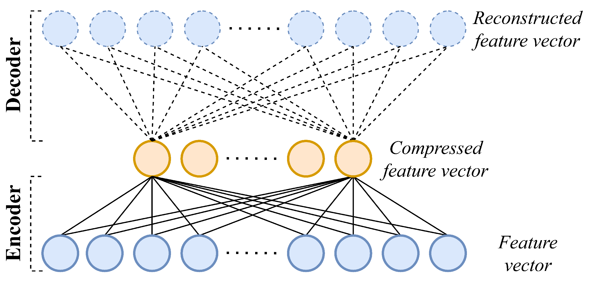
2.3. Autoencoder

Among current techniques for dimensionality reduction and information retrieval, an autoencoder (AE) is widely used not only as a nonlinear decomposition to replace traditional linear inner product but also as a representation learning mechanism [31]. It eliminates the information redundancy by mapping data from high feature space to lower one, generating more precise and efficient data representation.

Figure 1 illustrates the structure of a simple feedforward 1-layer AE. Generally, an AE is constituted by two main parts:

• An encoder $\varphi :𝒳\to 𝒞$ that maps the input features $𝒳$ into the code.
• A decoder $\psi :𝒞\to 𝒳$ that reconstructs the original features from the code.

The code $𝒞$ itself is the hidden layer output that is usually used to characterize the input. The objective of AE is to minimize the difference between the input and the output by reconstructing $𝒳$ from the reduced encoding $𝒞$ as follows:

$$\begin{array}{cc}\hfill \varphi ,\psi & =\underset{\varphi ,\psi }{arg\; min}{\parallel 𝒳-(\psi \circ \varphi )𝒳\parallel }^2\hfill \\ \hfill & =\underset{\varphi ,\psi }{arg\; min}{\parallel 𝒳-(\psi \left(\varphi \left(𝒳\right)\right)\parallel }^2\hfill \end{array}$$

(5)

In practice, only the code $𝒞$ is extracted to create a compressed representation of the input data that preserves the most crucial information for further analysis.

Several modifications on the AE architecture have been introduced recently to improve the effectiveness of representation learning and dimensionality reduction. To prevent the autoencoder from learning the identity function, Denoising Autoencoder (DAE) first corrupts the input by adding noise, then learns to predict the initial data point as the output [32]. Meanwhile, despite sharing a similar architecture with a vanilla AE, Variational Autoencoder (VAE) [33] encodes the input into a multivariate latent distribution rather than a vector.

There have been several studies successfully applying AE and its variants into RS. Collaborative Deep Learning (CDL) [34] was proposed for joint learning side information of items by a Stacked Denoising Autoencoder. Additionally, an AE-based model for rating prediction is the item-based AutoRec (I-AutoRec) [35] which fills missing ratings by applying an AE to reconstruct its input containing known ratings. In contrary to CDL, I-AutoRec directly handles explicit data to make reliable predictions without the side information. Other variations of AE [36,37] can also optimize the network input, capturing high-order latent factors from users and items.

3. Previous Work

In [38], a number of problems regarding similarity measurement method using the rating information were noticed. Firstly, the rating matrix in practice is extremely sparse (for example, 99.47% entries of this matrix in the MovieLens 20 M dataset are missing), which makes it hard to evaluate the relevance between two items that have many ratings but only share a few common users. Secondly, calculating the similarity score between two items is a time-consuming task due to a large number of users (usually in the order of millions). To address these problems, a novel similarity measure was proposed using Genome Tags instead of rating information. Specifically, each movie is characterized by a genome score vector $g=\{g_1,g_2,\cdots ,g_{1128}\}$ which encodes how strong a movie exhibits particular properties represented by 1128 tags [22], and the similarity score $s_{ij}$ between movies i and j is calculated as follows.

$$s_{g_i,g_j}^{Co{s}^{genome}}=\frac{{\sum }_{k=1}^G{g}_{ik}\times g_{jk}}{\sqrt{{\sum }_{k=1}^G{g}_{ik}^2}\times \sqrt{{\sum }_{k=1}^G{g}_{jk}^2}}$$

(6)

or

$$s_{g_i,g_j}^{PC{C}^{genome}}=\frac{{\sum }_{k=1}^G(g_{ik}-{\overline{g}}_i)\times (g_{jk}-{\overline{g}}_j)}{\sqrt{{\sum }_{k=1}^G{(g_{ik}-{\overline{g}}_i)}^2}\times \sqrt{{\sum }_{k=1}^G{(g_{jk}-{\overline{g}}_j)}^2}}$$

(7)

where ${\overline{g}}_i$ and ${\overline{g}}_j$ are the mean genome scores of vectors $g_i$ and $g_j$, respectively; and G = 1128 is the length of genome vectors. Experiments conducted on the preprocessed MovieLens 20 M dataset (keeping only movies with Tag Genome) showed that the item-oriented CF models based on similarity measures Cos_genome and PCC_genome provide accuracy equivalent to the state-of-the-art CF models using rating information whilst performing at least 2 times faster.

In [39], we introduced a natural language processing (NLP)-based cleaning process to eliminate the redundancy from the original 1128 genome tags to generate a more accurate description for each movie with 1044 new tags. While this process slightly improved the accuracy of the systems, the number of new tags is still quite large (7% smaller to original 1128 tags) and other groups of related tags which cannot be combined using NLP become hidden. Hence, a 3-layer AE was implemented to compress cleaned tags into a vector of 600 elements in order to discover the latent characteristics inside the genome tags and regenerate a more powerful representation of each movie. By using new feature vectors for every movie, kNN-Content^AE model can achieve at least 2.56% lower RMSE when compared to its counterparts while the prediction time is still reasonable.

Additionally, a novel technique integrating the matrix factorization output as the baseline estimate of user rating into kNNBaseline model was described as follows.

$${\widehat{r}}_{ui}^{kNN-Content}={\widehat{r}}_{ui}+\frac{{\sum }_{j\in {\mathrm{S}}^k(i;u)}{s}_{ij}\left(r_{uj}-{\widehat{r}}_{uj}\right)}{{\sum }_{j\in {\mathrm{S}}^k(i;u)}{s}_{ij}}$$

(8)

where ${\widehat{r}}_{ui}$ and ${\widehat{r}}_{uj}$ are the predicted ratings produced by SVD/SVD++ model while $s_{ij}$ is calculated by kNN-Content^AE model. This created hybrid content-based and CF models, kNN-Content^AE-SVD and kNN-Content^AE-SVD++, which take the advantages of both local level interaction of neighborhood-based method and global level characteristics explored by model-based method to provide more precise recommendations.

4. Experimental Setup

4.1. Dataset

In the literature, the two most popular datasets in recommendation system are the MovieLens dataset [22] and the Netflix Prize dataset [40]. While the former is continuously updated and complimented with new auxiliary knowledge for movies, the latter not only focuses on rating information associated with limited secondary data (only including movie’s title and year of release, and rating dates), but it has not been revised since the competition started due to privacy concerns. Therefore, in order to evaluate the performance of the proposed models, the MovieLens 20 M dataset is chosen as a benchmark in this work.

Released by GroupLens in 2015, this dataset originally contains 20,000,263 ratings and is updated in 2016 with the latest 465,564 tag applications across 27,278 movies created by 138,493 users (all selected users had rated at least 20 movies). The ratings range from 0.5 to 5.0 with a step of 0.5. Tag Genome data encodes how strongly movies exhibit particular properties represented by tags in the range of 0 to 1 which is computed using user-contributed content including tags, ratings, and textual reviews [22].

It is necessary to preprocess the original dataset. Any movie which does not have Tag Genome is discarded from the dataset. Only movies and users containing at least 20 ratings are kept.

Table 1. Summary of the original MovieLens 20 M and the preprocessed dataset.

	# Ratings	# Users	# Movies	Sparsity
Original dataset	20,000,263	138,493	27,278	99.47%
Preprocessed dataset	19,793,342	138,185	10,239	98.97%

summarizes the results: eventually, the preprocessed dataset consists of 19,793,342 ratings (approximately 98.97% sparsity compared to 99.47% sparsity of the original dataset) given by 138,185 users for 10,239 movies.

4.2. Evaluation Scheme

The preprocessed dataset is split into 2 distinct parts: 80% ratings of each movie are used as the training set, and the 20% remaining as the testing set. To compare the performance between models, the following widely-used indicators are used:

• RMSE (Root Mean Squared Error) for rating prediction task: evaluate the errors of the predicted ratings where smaller values provide more accurate recommendations:

  $$\mathrm{RMSE}=\sqrt{\sum _{u,i\in \mathrm{TESTSET}}{\left({\widehat{r}}_{ui}-r_{ui}\right)}^2/\left|\mathrm{TESTSET}\right|}$$

  (9)

  where $\left|\mathrm{TESTSET}\right|$ is the size of the testing set, ${\widehat{r}}_{ui}$ denotes the predicted rating of user u to item i estimated by the model, and the corresponding observed rating in the testing set is denoted by $r_{ui}$.
• Precision@k (P@k) and Recall@k (R@k) for the ranking (top-k recommendation) task: Precision@k is defined as a fraction of relevant items among the top k recommended items, and Recall@k is defined as a fraction of relevant items in the top k recommended items among all relevant items. Higher P@k and R@k indicate that more relevant items are recommended to users.
• Time [s] for timing evaluation: the total duration of the model’s learning process on the training set and predicting all samples in the testing set.

All experiments in this work are conducted on a workstation consisting of an Intel Xeon Processor E5-2637 v3 3.50 GHz (2 processors) with 32 GB RAM and no GPU.

4.3. Baselines and Experimental Settings

To evaluate the performance of proposed models, the following baseline models are implemented.

• ii-CF [24]: the similarity score between movies is measured using PCCBaseline with the number of neighbors is set at 40.
• SVD [6] and SVD++ [7]: both models are trained using 40 hidden factors with 100 iterations and the step size of 0.002.
• NMF: optimization procedure is a regularized SGD based on Euclidean distance error function [41] with regularization strength of 0.02 and 40 hidden factors.
• kNN-Content [38]: PCC_genome is used as the similarity measure.
• kNN-Content^AE-SVD and kNN-Content^AE-SVD++ [39]: 600-feature vectors for movies are learned from 1044 NLP-preprocessed genome tags using a 3-layer AE.
• FM_genome [14]: each feature vector is composed of one-hot encoded user and movie ID, movie genres and genome scores associated with each movie; the model is trained with degree $d=2$ and 50 iterations.
• I-AutoRec [35]: a 3-layer AE is trained using 600 hidden neurons, and the combination of activation functions is $(Identity,Sigmoid)$.

In our experiments, the optimal hyperparameters for each baseline method above are carefully selected using 5-fold cross validation to guarantee fair comparisons. For ii-CF model, the number of neighbors is chosen from {10, 20, 30, 40, 50, 100, 150}, and the similarity measures implemented are Cos, PCC and PCCBaseline. For SVD, SVD++, and NMF models, the number hidden factors is chosen from {20, 30, 40, 50, 60, 80, 100}. These traditional models are reimplemented using Numba compiler (https://github.com/numba/numba, accessed on 2 November 2021) to optimize their performances [42]. For I-AutoRec model, the size of the hidden layer is set for n ∈ {200, 400, 600, 800, 1000} units; and the choices of activation functions $f(·),g(·)$ are experimented with $(Identity,Identity)$, $(Identity,Sigmoid)$, $(Sigmoid,Identity)$, $(Sigmoid,$$Sigmoid)$. Finally, the regularization strength is tuned $\lambda \in \{0.001,0.002,0.01,$$0.02,0.1,1,2\}$ for all baselines.

In this paper, we have two main contributions. In the following, a novel autoencoder named Half Convolutional Autoencoder is first introduced to capture the fundamental characteristics of each movie from its original Tag Genome. The ability to extract essential features of an HCAE is empirically proven to outperform that of the classical AE and its variants via the application in various RSs. Secondly, through the newly generated representation for each movie, a user’s interest is vectorized by the movies she rated. Both the movie and user vectors are then adopted to initialize the latent vectors in matrix factorization models, which significantly boosts the precision of the systems.

5. Half Convolutional Autoencoder

5.1. Learning New Representation of Structured Data with an HCAE

Experimental results in our previous work [39] demonstrated the capability of an AE to produce a more compact and powerful representation for movies than the original genome scores. However, the fully-connected architecture of a traditional AE does not consider the order of its raw inputs, which takes a risk that the network just tries to learn the data without extracting any more useful information [19].

Compared to conventional fully connected neural networks, a typical CNN does not require a large number of neurons for high dimensional inputs, which enables the training process to be much more efficient with fewer parameters. Additionally, CNNs are widely recognized as a robust feature extractor that is commonly applied on unstructured data such as images, videos or audio where elements of a data point spatially and/or temporally close to each other share similar information, and their positioning can negatively affect the performance if arranged arbitrarily [43].

Meanwhile, data in common RSs are mostly stored in tabular form such as rating matrix, user profiles, or movie genres (for example, the MovieLens datasets). This kind of structured data has generally little or no spatial/temporal knowledge and is considered to be suitable for fully connected networks. Hence, to our knowledge, there is little effort in applying a CNN as the feature extractor in RSs despite its effectiveness.

As stated above, this paper focuses on the MovieLens 20 M dataset which introduces a new type of information associated with each movie named Tag Genome. Investigating this kind of tabular data provides us some prospective reasons for applying a CNN in order to generate a more precise representation for each movie against a vanilla AE:

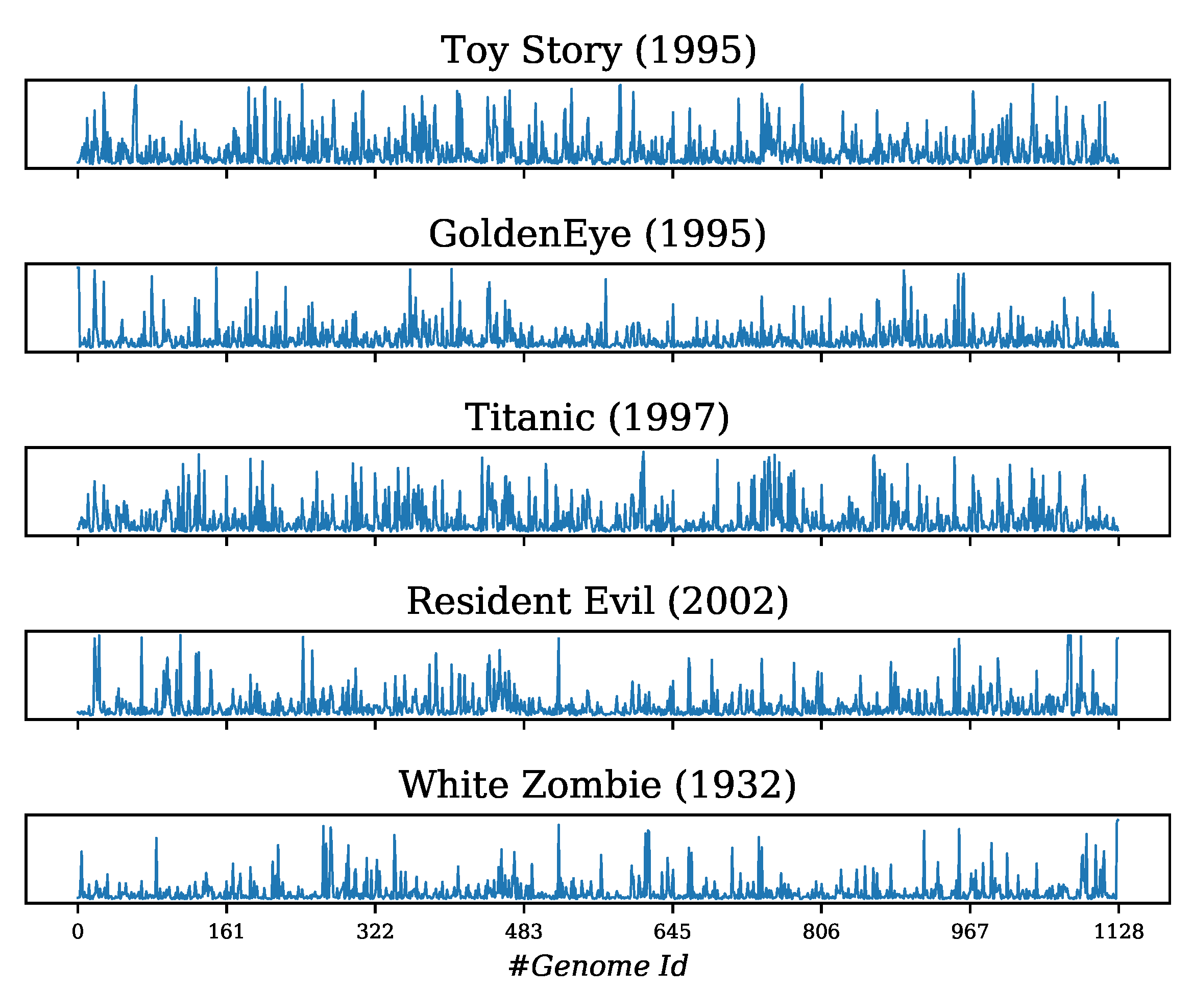
• Firstly, we reorganize Tag Genome data into a table so that each movie is represented as a row and its genome scores are stored in the columns (as in

  Table 2. Reorganizing original Tag Genome data into a tabular form. Each movie is presented as a row and its genome scores are stored in the columns.

  	Tag #1	Tag #2	Tag #3	⋯	Tag #1127	Tag #1128
  Toy Story (1995)	0.0250	0.0250	0.0578	⋯	0.0778	0.0230
  GoldenEye (1995)	0.9998	0.9998	0.0195	⋯	0.0730	0.0183
  Titanic (1997)	0.0380	0.0345	0.1190	⋯	0.0693	0.0210
  Resident Evil (2002)	0.0403	0.0350	0.0195	⋯	0.9588	0.9598
  White Zombie (1932)	0.0188	0.0203	0.0270	⋯	0.9670	0.9840
  ⋯	⋯	⋯	⋯	⋯	⋯	⋯

  ). It can be seen that each row has fully numerical values in the range of $[0,1]$ which indicate the strength of the relevance between a movie and its corresponding genome tags (i.e., attributes). If each row is assumed to be a discrete-time signal where the attributes’ positions are treated as “timestamps” and their values as the displacements, each movie will be characterized by a signal bringing its information. Moreover, the attributes are generally independent of each other, so this signal resembles a random vibration illustrated in Figure 2 that we could apply a 1D-CNN to extract its features [44].
• Secondly, if the order of the columns is shuffled simultaneously for all movies, the physical shapes of the signals will change in a consistent way (i.e., the correlation between a random pair of signals remains unchanged) and still deliver the knowledge about the movies. In other words, the above assumption holds true regardless of the positioning of the movie attributes into the table. Consequently, a 1D-CNN still has the potential to perform feature extraction on the new signals.

We also tried to apply a 2D-CNN on these “vibration” signals using a proper 1D-to-2D conversion. A common technique is to reshape the signals into $m\times n$ matrices before feeding them into a 2D-CNN [45,46]. Nonetheless, this technique requires the length of the input signals to be a non-prime number and often costs a higher computational complexity than its 1D counterpart. Therefore, we opt to choose a 1D-CNN for our purpose.

In this work, a novel autoencoder architecture named Half Convolutional Autoencoder is devised to harness the capability of a 1D-CNN in order to explore the essential characteristics of the movies from the available Tag Genome data. The structure of an HCAE is illustrated in Figure 3. Specifically, a complete forward-propagation process of HCAE can be described in the following steps:

1.

A feature vector representing a random vibration signal is fed to the input layer of the HCAE;

2.

Each neuron of the 1D-Convolution layer performs a linear convolution between the signal and corresponding filter to generate the input feature map of the neuron;

3.

The input feature map of each neuron is passed through the activation function to generate the output feature map of the neuron of the convolution neuron;

4.

In the 1D-Pooling layer, each neuron’s feature map is created by decimating the output feature map of the previous neuron of the 1D-Convolution layer to reduce the dimensions of the final feature maps;

5.

In the Flatten layer, the output feature maps are flattened into a single feature vector, which is forward-propagated through the following fully-connected Compression layer to encode the feature map into lower dimensional space;

6.

The decoder structure remains fully connected like a vanilla AE, where the output code are forward-propagated through a fully connected decoder to reconstruct the original feature vector, or the 1D-signal.

Compared to a typical AE, the fundamental difference of the HCAE comes from the asymmetry of the Half Convolutional encoder and decoder parts, hence its name.

In more detail, the encoder part of the newly proposed architecture works as follows. For each filter $F_i$, the 1D-Convolution layer, along with the 1D-Max Pooling layer, learns the feature map $d_i=P\left(g(\mathcal{X}*F_i)\right)$ from input feature vector $𝒳$, where $g(*)$ is the activation function of the Convolution layer, and $P(*)$ denotes the Max Pooling transformation. These feature maps are then transformed to a 1D-vector $\mathbf{d}$ via a Flatten layer before eventually being fed into a Compression layer to generate a compact representation of a movie. Here the output sizes of the Convolution layer $n_{out}$ with the padding size p and of the Max Pooling layer $n_{out}^{\prime }$ are calculated using the following formulas:

$$n_{out}=\left(\frac{n_{in}+2p-f}{s}\right)+1$$

(10)

$$n_{out}^{\prime }=\left(\frac{n_{in}^{\prime }-f^{\prime }}{s^{\prime }}\right)+1$$

(11)

where $n_{in}$, $n_{in}^{\prime }$ denote the input sizes; f, $f^{\prime }$ are the kernel sizes; and s, $s^{\prime }$ are the stride sizes of the Convolution and Max Pooling layers, respectively.

Although the encoder implements a CNN architecture, the decoder works similarly to the one of a conventional AE: it tries to reconstruct the original input through a fully connected layer. In addition to possessing the same objective function as the one of a vanilla AE, this structure makes the proposed HCAE easily adapt to any shape of the input vector, which is infeasible if a 1D-Up Sampling layer is deployed at the decoder in the case of a “full” Convolutional AE. That is due to the fact that the output size of a 1D-Up Sampling layer is computed as:

$$n_{UpSampling\_out}=n_{UpSampling\_in}\ast f_{UpSampling}$$

(12)

where $n_{UpSampling\_in}$ and $f_{UpSampling}$ denote the input size and the factor size of the layer, respectively. It is implied that Equation (12) imposes certain constraints on the values of these 3 factors. For instance, $n_{UpSampling\_out}$ must be a non-prime; otherwise, $n_{UpSampling\_in}$ has to be equal to $n_{UpSampling\_out}$ and $f_{UpSampling}$ equal to 1, which is almost meaningless. It is worth noting that $n_{UpSampling\_in}$ matches the length of the Max Pooling layer’s output, and $n_{UpSampling\_out}$ is exactly the original input size of the HCAE. Therefore, this causes restrictions on the input shape as well as the hyperparameter selection of the proposed architecture.

5.2. Utilizing HCAE in Recommendation Systems

In our experiments, the number of filters and the kernel size of the Convolution layer are firstly configured at 4 and 5, respectively. However, we later show that the overall performance of the HCAE is almost not affected by the values of these settings. The pooling size and the stride size are set equal to the number of filters so that the output of the Flatten layer has the same dimension as the HCAE input. Comprehensive experiments show that the dropout rate of 0.2 between the Compression and the Output layer is effective in preventing overfitting. The optimization algorithm used in this work is $Adam$ due to little hyperparameter-tuning requirement, computational efficiency and faster convergence [47].

Activation of the decoder is $Sigmoid$ function which returns the value between 0 and 1 to match the range of the genome scores. To find the optimal activations for the Convolution and Compression layers, a variety of functions, including $Identity$, $ReLU$ and $Sigmoid$, are examined. Baseline model kNN-Content in Section 4.3 is used to assess the quality of the compressed genome scores. In more detail, 1128 genome scores of each movie are fed into the HCAE in order to extract its most fundamental features which are employed to calculate PCC_genome similarity between movies in kNN-Content model using Equation (7) with $k=10$.

Table 3. Performance of kNN-Content model with different activation functions of the Convolution and Compression layers in the HCAE.

Activation Function		RMSE	Time [s]
Convolution Layer	Compression Layer
Identity	Identity	0.7856	295
Identity	ReLU	0.7608	297
Identity	Sigmoid	0.7638	298
ReLU	Identity	0.7854	296
ReLU	ReLU	0.7739	297
ReLU	Sigmoid	0.7641	300
Sigmoid	Identity	0.7976	298
Sigmoid	ReLU	0.7932	299
Sigmoid	Sigmoid	0.7678	302

illustrates the performance of various activations in the case of compressing Tag Genome to $N=600$ features, where only RMSE are shown for brevity. Experiments with different values of N provide the same results: a combination of $(Identity,ReLU)$ provides the lowest error rate and is chosen for the Half Convolutional encoder thereafter.

To thoroughly evaluate the capability of the HCAE against other AE architectures, both versions of genome tags, 1128 original and 1044 combined ones using NLP [39], are chosen as their inputs. Specifically, a vanilla AE and its two popular variants are implemented as follows:

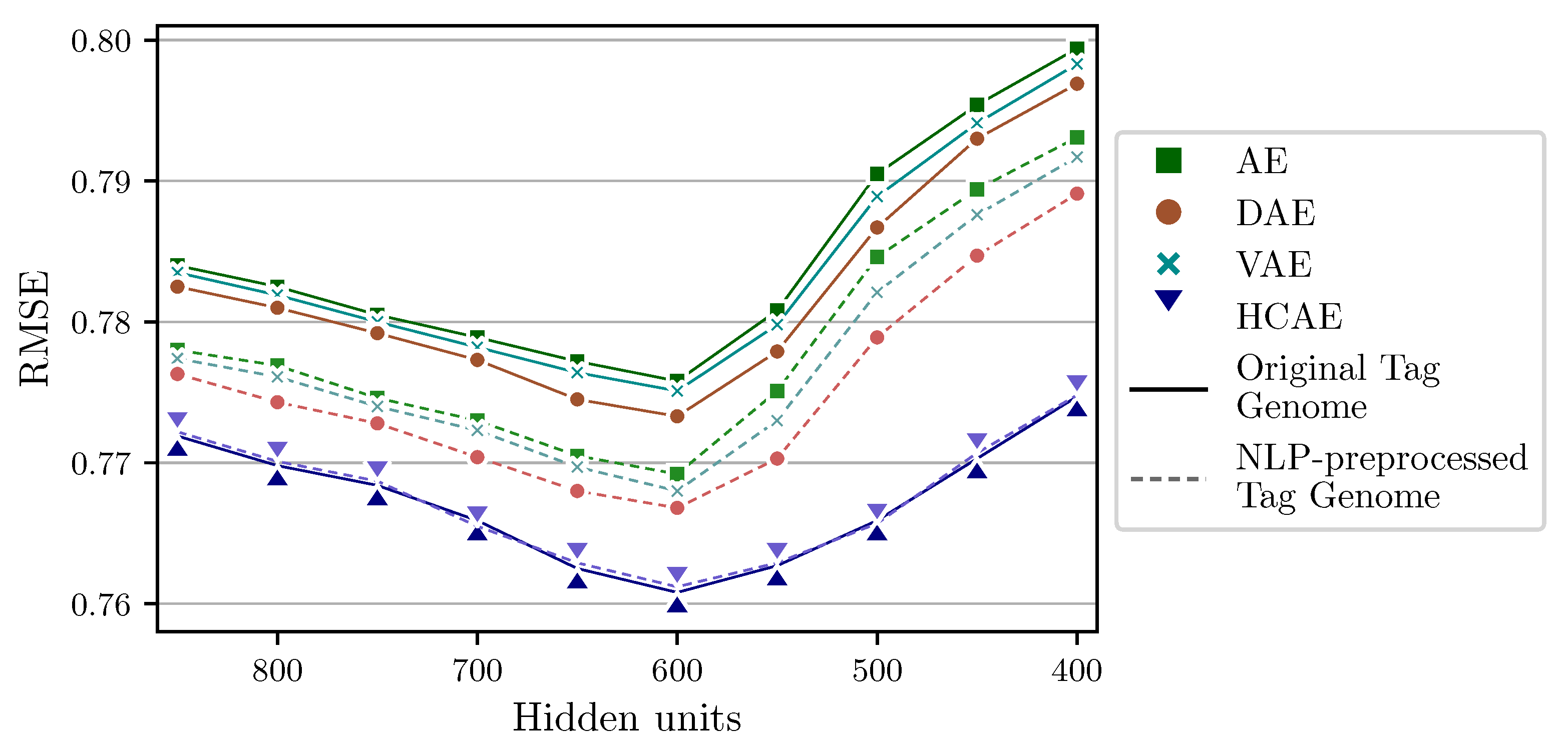
• AE: a 3-hidden layer AE that uses $ReLU$ activation function at all hidden layers and $Sigmoid$ activation function at the output layer; the number of units at hidden layers $\#1$ and $\#3$ is fixed at 900;
• DAE: a 1-hidden layer DAE with $noise\_factor=0.1$ that uses $ReLU$ activation function at the hidden layer and $Sigmoid$ activation function at the output layer;
• VAE: a 4-hidden layer VAE is configured as follows: 900-unit hidden layers $\#1$ and $\#4$ use $ReLU$ activation function; Compression layer constructed from $Mean$ layer and $Var$ layer use $Linear$ activation function; $Sigmoid$ activation function is used for output layer.

In our experiments, the proposed HCAE and its counterparts are deployed with different sizes of Compression layer to find the optimal configuration for each model. All models are trained until saturation using Adam optimization algorithm and the learning rate of 0.001. Figure 4 shows that although all AE architectures achieve the highest quality with the Compression layer of 600 units, they perform differently for two types of inputs: whilst the classic AE and its two well-known variants do not work well with the original tags, the proposed architecture operates almost equivalently regardless of whether the inputs are preprocessed or not. Furthermore, the HCAE proves superior in extracting essential features over its competitors for both cases. This suggests that the HCAE has the potential of discovering the hidden relationships under the original genome tags without the need of analyzing their semantic meanings, which helps to ignore the NLP-based preprocess. In more general situations, it is expected that the HCAE still demonstrates its virtue with various kinds of input, not limited to data with meaningful labels. Hence, the 1128 original genome tags are selected for the remaining experiments hereafter.

During the training process, we try shuffling the order of the genome scores as well as examining different values of the number of filters $(2,4,6,12,20)$ and the kernel sizes $(3,5,7,11,19,29)$ for the Convolution layer. Although the outputs of the Flatten and Compression layers vary constantly through the experiments, empirical results show that choosing the configuration of 4 filters and the kernel size of 5 provides the most accurate predictions in the final model but does not have a considerable improvement over other choices (the error rates fluctuate less than 0.06%). This result helps to confirm our initial hypothesis that the Half Convolutional encoder could derive latent characteristics from the input data irrespective of the relationship and the positioning of the movie attributes.

For a more comprehensive evaluation, 600-feature vectors for movies generated from different types of AE are then applied into a number of baseline models: kNN-Content, FM_genome, kNN-Content-SVD, and kNN-Content-SVD++. It is noteworthy that in the cases of AE/DAE/VAE, feature vectors are compressed from the 1044 NLP-preprocessed genome tags for fair comparison because it provides better movie representation than using the original tags. In

Table 4. Performance comparison of the baseline models when utilizing 600-element movie feature vectors generated from AE variants and an HCAE.

Model	Auto Encoder	RMSE	P@5	P@10	R@5	R@10	Time [s]
kNN- Content	AE	0.7692	0.8142	0.7906	0.4352	0.5587	289
		(−1.09%)	(+0.68%)	(+0.79%)	(+0.55%)	(+0.68%)
	VAE	0.7680	0.8137	0.7914	0.4358	0.5592	316
		(−0.94%)	(+0.74%)	(+0.69%)	(+0.41%)	(+0.59%)
	DAE	0.7668	0.8147	0.7925	0.4355	0.5588	291
		(−0.78%)	(+0.62%)	(+0.55%)	(+0.48%)	(+0.66%)
	HCAE	0.7608	0.8198	0.7969	0.4376	0.5625	297
FMgenome	AE	0.7702	0.8052	0.7836	0.4300	0.5571	23,412
		(−0.87%)	(+0.62%)	(+0.72%)	(+0.78%)	(+0.71%)
	VAE	0.7688	0.8057	0.7841	0.4295	0.5578	23,535
		(−0.69%)	(+0.56%)	(+0.66%)	(+0.90%)	(+0.59%)
	DAE	0.7681	0.8063	0.7852	0.4310	0.5587	23,447
		(−0.60%)	(+0.48%)	(+0.52%)	(+0.55%)	(+0.43%)
	HCAE	0.7635	0.8102	0.7893	0.4334	0.5611	23,503
kNN- Content- SVD	AE	0.7634	0.8162	0.7946	0.4356	0.5575	596
		(−0.98%)	(+0.78%)	(+0.76%)	(+0.53%)	(+0.78%)
	VAE	0.7623	0.8166	0.7941	0.4349	0.5580	653
		(−0.84%)	(+0.73%)	(+0.82%)	(+0.68%)	(+0.69%)
	DAE	0.7612	0.8177	0.7954	0.4355	0.5594	603
		(−0.70%)	(+0.60%)	(+0.66%)	(+0.55%)	(+0.44%)
	HCAE	0.7559	0.8226	0.8007	0.4379	0.5619	612
kNN- Content- SVD++	AE	0.7584	0.8186	0.7959	0.4368	0.5609	27,687
		(−0.90%)	(+0.78%)	(+0.90%)	(+0.66%)	(+0.69%)
	VAE	0.7569	0.8191	0.7962	0.4363	0.5610	27,761
		(−0.70%)	(+0.72%)	(+0.86%)	(+0.77%)	(+0.67%)
	DAE	0.7560	0.8198	0.7972	0.4374	0.5617	27,698
		(−0.58%)	(+0.63%)	(+0.73%)	(+0.52%)	(+0.55%)
	HCAE	0.7516	0.8250	0.8031	0.4397	0.5648	27,737

, the relative improvements of the HCAE-based models over their counterparts are displayed in the parentheses under the corresponding accuracy indicators. Here, +/− signs indicate that the indicators of the proposed models are “greater”/“less” than the ones of their competitors, where the lower the RMSE or the higher the Precision/Recall the model gets, the better the performance is. This notation is also applied in the rest of this paper. Experimental results show that kNN-Content^HCAE model gains the largest decreases in RMSE compared to kNN-Content^AE model by 1.09% while also achieving at least 0.55% improvement in Precision/Recall. The other HCAE-based models also outperform their AE counterparts by at least 0.53% at the expense of operating time. Similar results can be seen when comparing HCAE- against DAE- and VAE-based models. A remarkable point here is that DAE performs better than AE and VAE in extracting fundamental features for movies. A potential reason for the dominance of DAE is its ability to process “noisy” genome scores calculated from user-contributed tags which possibly suffer from artificial errors. Even though the proposed HCAE still yield 0.58–0.78% lower RMSE and 0.43–0.73% higher Precision/Recall than DAE in all models.

It is worth noting that the operating time of AE/DAE/VAE here does not take into account the step of NLP preprocessing which is totally eliminated when utilizing the proposed HCAE. In practice, the preprocessing stage introduced in [39] may cost a great amount of time if the number of tags increases sharply, which is highly likely to happen because they are freely generated by users. Therefore, the trade-off is totally acceptable.

6. Novel Initialization Method Using Content-Based Information for Matrix Factorization Techniques

As introduced in Section 2.2, matrix factorization is a well-known technique for discovering latent features. Although this technique performs well on extremely sparse data such as rating matrix, it lacks explainability: latent factors achieved after training a matrix factorization model are most likely uninterpretable. Furthermore, traditional matrix factorization methods randomly initialize user and item vectors during the training process that may lead to slow convergence. Especially, NMF is greatly affected by the initialization: if the initial values of $p_u$ and $q_i$ are not good, it is more likely that the training will be unstable, and even unable to converge [11,48]. Recent years have witnessed a large number of efforts to eliminate these problems. One of the highly promising approaches is to initialize the latent vectors with more meaningful values [15,16].

In this paper, a new method of initialization in matrix factorization is proposed: instead of learning user and item features from randomly valued vectors, we attempt to integrate both content- and rating-based information into the initial vectors. Currently, one of the common ways to describe user preferences is using the interactions that a user assigned to the movies she watched. However, by using this method, rating data and movie attributes are treated independently, which may cause a huge waste of information. To tackle this issue, a new way of generally profiling a user that incorporates content-based data of all the movies she rated is introduced as follows.

$$P_u=\frac{1}{\left|R\right(u\left)\right|}\sum _{i\in R\left(u\right)}({\tilde{r}}_{ui}\times Q_i)$$

(13)

where ${\tilde{r}}_{ui}$ denotes the rating user u gave to movie i which has been normalized to the range of $[0,1]$, and $Q_i$ is the feature vector of movie i that reflects its content-related information. Recall that $R\left(u\right)$ denotes the set of all movies rated by user u. In such a manner, a user vector $P_u$ has the same dimension and range of values as a movie vector $Q_i$. More importantly, each user is characterized in an explainable way: elements with grearer values indicate that the user has a greater preference for the respective movie attributes and vice versa.

Finally, both the user and movie latent features of the matrix factorization model are initialized using the vectors $P_u$’s and Q_i’s described above. During the scope of this work, the Tag Genome is utilized to demonstrate the content of each movie. In order to comprehensively evaluate the new method of initialization, different representations of a movie based on these metadata are experimented: the 1128 original genome tags, the shortened 1044 ones using NLP [39], and the two 600-element feature vectors generated using the newly proposed HCAE and the DAE which yield the best results in the previous section. We refer to the proposed models with -genome suffix to indicate that the user and movie genome scores are integrated into the learning process where the number of latent factors k must match the dimension of corresponding feature vectors. In our experiments, SVD-genome and NMF-genome models are trained with the learning rate of 0.005 and the regularization strength of 0.02. The randomly initialized counterparts are trained 20 times using the same hyperparameters to select the most precise models for comparison. For clarity, we only include RMSE in

Table 5. Performance comparison between randomly initialized matrix factorization models and their custom initialized counterparts integrating user and movie feature vectors.

Model	RMSE	Epochs	Time [s]
NMF ($k=1128$)	0.7993	305	32,115
NMF-genome	0.7797	200	21,220
(1128 original scores)	(−2.45%)	(−34.43%)	(−33.92%)
NMF ($k=1044$)	0.7987	290	18,802
NMF-genome	0.7792	165	10,843
(1044 NLP-preprocessed scores)	(−2.44%)	(−43.10%)	(−42.33%)
NMF ($k=600$)	0.7984	265	9,937
NMF-genome	0.7718	125	4695
(600 scores of DAE)	(−3.33%)	(−52.83%)	(−52.75%)
NMF-genome	0.7688	97	3729
(600 scores of HCAE)	(−3.71%)	(−63.40%)	(−62.47%)
SVD ($k=1128$)	0.7930	230	11,201
SVD-genome	0.7582	55	2713
(1128 original scores)	(−4.39%)	(−76.09%)	(−75.78%)
SVD ($k=1044$)	0.7927	150	5895
SVD-genome	0.7547	45	1787
(1044 NLP-preprocessed scores)	(−4.79%)	(−70.00%)	(−69.69%)
SVD ($k=600$)	0.7925	140	3018
SVD-genome	0.7536	35	905
(600 scores of DAE)	(−4.91%)	(−75.00%)	(−70.01%)
SVD-genome	0.7472	30	814
(600 scores of HCAE)	(−5.72%)	(−78.57%)	(−73.03%)

.

As displayed in Table 5, incorporating rating data and movie attributes into the initialization significantly boosts SVD-genome and NMF-genome models over their original versions. In detail, the proposed models show an exceptionally faster convergence rate against the competitors in all experiments: the training time measured by the number of epochs is reduced to at least 34.43%, especially up to 63.40% and 78.57% with the models utilizing HCAE-generated feature vectors. At the same time, SVD-genome and NMF-genome models totally outperform their corresponding counterparts from 2.44% to 5.72% in RMSE. Once again, it can be seen that initializing latent vectors with 600 scores produced by an HCAE (highlighted rows) provides the lowest error rate when compared with other representations, which further proves the superiority of the HCAE against AE variants stated in the previous section. These remarkable improvements prove that learning the user and item latent features from appropriate initial vectors could greatly benefit matrix factorization models: it not only helps the training process to converge faster but also enhances the accuracy. In real-life applications, the word “appropriate” here implies that we could take advantage of all accessible knowledge including user preferences and available metadata, not limited to user-contributed genome tags in the above experiments, in order to characterize user and item features as precisely as possible. This empirical result suggests that the more meaningful values of initial latent vectors, the more likely it is to achieve better matrix factorization-based RSs in terms of precision and computational complexity.

Another advantage of the newly proposed method is that if adopting the original 1128 genome tags or the shortened 1044 ones preprocessed by NLP for initialization, movie latent vectors generated after training have much better interpretability than the ones from traditional matrix factorization models. As demonstrated in Figure 5, the most relevant tags of Titanic (1997) deduced from the learned movie features are highly reasonable for both versions of the genome tags. For user latent vectors, there are clear differences before and after training (user with $id=1$ for example). However, it is reasonable to expect that learned user vectors could provide a better understanding of user preferences and can be employed for further analysis owing to their significant contribution towards generating RSs with higher accuracy.

The two most accurate models, NMF-genome and SVD-genome utilizing 600 HCAE-generated scores, are chosen to compare with the baselines listed in Section 4.3. In this final experiment, the baselines are implemented using different libraries and frameworks in order to pick up the model with the lowest error rate, not considering the overall time to finish the training and predicting process. In other words, we only evaluate the models in terms of accuracy. Therefore, only accuracy indicators are displayed in

Table 6. Performance comparison between the proposed models utilizing 600 HCAE-generated feature vectors and the baseline models.

Model	RMSE	P@5	P@10	R@5	R@10
ii-CF	0.8046	0.7967	0.7721	0.4261	0.5541
	(−7.13%)	(+4.06%)	(+4.45%)	(+3.79%)	(+3.20%)
I-AutoRec	0.7808	0.7778	0.7559	0.3972	0.5228
	(−4.30%)	(+6.33%)	(+6.46%)	(+10.32%)	(+8.67%)
NMF	0.7981	0.7951	0.7743	0.4296	0.5583
	(−6.38%)	(+4.25%)	(+4.18%)	(+3.00%)	(+2.46%)
SVD	0.7922	0.8005	0.7786	0.4322	0.5628
	(−5.68%)	(+3.60%)	(+3.65%)	(+2.42%)	(+1.68%)
SVD++	0.7894	0.8030	0.7817	0.4339	0.5639
	(−5.35%)	(+3.30%)	(+3.27%)	(+2.03%)	(+1.48%)
kNN-ContentHCAE-SVD	0.7559	0.8226	0.8007	0.4379	0.5619
	(−1.15%)	(+0.94%)	(+0.92%)	(+1.13%)	(+1.83%)
kNN-ContentHCAE-SVD++	0.7516	0.8250	0.8031	0.4397	0.5648
	(−0.59%)	(+0.65%)	(+0.62%)	(+0.72%)	(+1.33%)
NMF-genome	0.7688	0.8174	0.7941	0.4389	0.5689
	(−2.81%)	(+1.57%)	(+1.73%)	(+0.90%)	(+0.61%)
SVD-genome	0.7472	0.8304	0.8081	0.4429	0.5724

for fair comparison. Experimental results show that the proposed models greatly surpass the competitors. Specifically, the highlighted winning model, SVD-genome, has gained an improvement from approximately 0.59% to 7.13% over the baselines at both rating prediction and ranking tasks. These results are encouraging, and it is highly likely that a much lower error rate could be attained if the proposed initialization method is applied to SVD++ and its current state-of-the-art variants such as timeSVD++ [8] and flippedTimeSVD++ [49]. However, due to our limited hardware resources, this experiment cannot be carried out: using a large number of latent factors causes the training process to take an enormous amount of time to finish. In real-life applications, this huge trade-off between accuracy and computational complexity is usually not worth the effort.

7. Conclusions

In this work, a novel architecture of autoencoder named HCAE is first proposed in order to discover essential information from the original Tag Genome of each movie. By integrating a 1D-CNN into the encoder part, an HCAE proves its capability in feature extraction compared to a vanilla AE and its variants, especially without the need for the time-consuming data preprocessing stage. Secondly, a new method of profiling users is introduced using the HCAE-generated movie feature vectors and rating information. The new representations of users and movies are then utilized as the initial latent vectors during the training stage of common matrix factorization techniques. In addition to learning movie feature vectors with better explainability, experimental results demonstrate that the custom-initialized SVD/NMF models not only converge much faster in the training but also outperform the randomly initialized counterparts in both rating prediction and ranking tasks. It is thus expected that matrix factorization-based RSs could be greatly improved via generating robust user and item profiles from all available information for initialization.

The proposed HCAE has enabled several potential ideas on applying state-of-the-art feature extractors such as a deep CNN or a transformer-based AE to generate robust hidden feature vectors. Another potential direction is to adopt convolutional or transformer-based models not only as an AE, but as an end-to-end recommendation model.

References

- Adomavicius, G.; Tuzhilin, A. Toward the next generation of recommender systems: A survey of the state-of-the-art and possible extensions. IEEE Trans. Knowl. Data Eng. 2005, 17, 734–749. [Google Scholar] [CrossRef]
- Lops, P.; De Gemmis, M.; Semeraro, G. Content-based recommender systems: State of the art and trends. In Recommender Systems Handbook; Springer: Cham, Switzerland, 2011; pp. 73–105. [Google Scholar]
- Narducci, F.; Basile, P.; Musto, C.; Lops, P.; Caputo, A.; de Gemmis, M.; Iaquinta, L.; Semeraro, G. Concept-based item representations for a cross-lingual content-based recommendation process. Inf. Sci. 2016, 374, 15–31. [Google Scholar] [CrossRef]
- Su, X.; Khoshgoftaar, T.M. A Survey of Collaborative Filtering Techniques. Available online: https://downloads.hindawi.com/archive/2009/421425.pdf (accessed on 2 November 2021).
- Ricci, F.; Rokach, L.; Shapira, B. Recommender systems: Introduction and challenges. In Recommender Systems Handbook; Springer: Cham, Switzerland, 2015; pp. 1–34. [Google Scholar]
- Funk, S. Netflix Update: Try This at Home. 2006. Available online: https://sifter.org/simon/journal/20061211.html (accessed on 2 November 2021).
- Koren, Y. Factorization meets the neighborhood: A multifaceted collaborative filtering model. In Proceedings of the 14th ACM SIGKDD International Conference on Knowledge Discovery and Data Mining, Las Vegas, NV, USA, 24–27 August 2008; pp. 426–434. [Google Scholar]
- Koren, Y. Collaborative filtering with temporal dynamics. In Proceedings of the 15th ACM SIGKDD International Conference on Knowledge Discovery and Data Mining, Paris, France, 28 June–1 July 2009; pp. 447–456. [Google Scholar]
- Wild, S.; Curry, J.; Dougherty, A. Improving non-negative matrix factorizations through structured initialization. Pattern Recognit. 2004, 37, 2217–2232. [Google Scholar] [CrossRef]
- Boutsidis, C.; Gallopoulos, E. SVD based initialization: A head start for nonnegative matrix factorization. Pattern Recognit. 2008, 41, 1350–1362. [Google Scholar] [CrossRef] [Green Version]
- Albright, R.; Cox, J.; Duling, D.; Langville, A.N.; Meyer, C. Algorithms, Initializations, and Convergence for the Nonnegative Matrix Factorization. Available online: https://www.ime.usp.br/~jmstern/wp-content/uploads/2020/04/Albright1.pdf (accessed on 2 November 2021).
- Agarwal, D.; Chen, B.C. Regression-based latent factor models. In Proceedings of the 15th ACM SIGKDD International Conference on Knowledge Discovery and Data Mining, Paris France, 28 June–1 July 2009; pp. 19–28. [Google Scholar]
- Barragáns-Martínez, A.B.; Costa-Montenegro, E.; Burguillo, J.C.; Rey-López, M.; Mikic-Fonte, F.A.; Peleteiro, A. A hybrid content-based and item-based collaborative filtering approach to recommend TV programs enhanced with singular value decomposition. Inf. Sci. 2010, 180, 4290–4311. [Google Scholar] [CrossRef]
- Rendle, S. Factorization machines. In Proceedings of the 2010 IEEE International Conference on Data Mining, Sydney, Australia, 13–17 December 2010; pp. 995–1000. [Google Scholar]
- Hidasi, B.; Tikk, D. Initializing Matrix Factorization Methods on Implicit Feedback Databases. J. UCS 2013, 19, 1834–1853. [Google Scholar]
- Zhao, J.; Geng, X.; Zhou, J.; Sun, Q.; Xiao, Y.; Zhang, Z.; Fu, Z. Attribute mapping and autoencoder neural network based matrix factorization initialization for recommendation systems. Knowl. Based Syst. 2019, 166, 132–139. [Google Scholar] [CrossRef]
- He, X.; Liao, L.; Zhang, H.; Nie, L.; Hu, X.; Chua, T.S. Neural Collaborative Filtering. In Proceedings of the 26th International Conference on World Wide Web, International World Wide Web Conferences Steering Committee, Republic and Canton of Geneva, Geneva, Switzerland, 3–7 April 2017; pp. 173–182. [Google Scholar]
- Martins, G.B.; Papa, J.P.; Adeli, H. Deep learning techniques for recommender systems based on collaborative filtering. Expert Syst. 2020, 37, e12647. [Google Scholar] [CrossRef]
- LeCun, Y.; Bengio, Y. Convolutional Networks for Images, Speech, and Time Series. Available online: www.iro.umontreal.ca/lisa/pointeurs/handbook-convo.pdf (accessed on 2 November 2021).
- Abdul, A.; Chen, J.; Liao, H.Y.; Chang, S.H. An emotion-aware personalized music recommendation system using a convolutional neural networks approach. Appl. Sci. 2018, 8, 1103. [Google Scholar] [CrossRef] [Green Version]
- Kim, D.; Park, C.; Oh, J.; Lee, S.; Yu, H. Convolutional matrix factorization for document context-aware recommendation. In Proceedings of the 10th ACM Conference on Recommender Systems, Boston, MA, USA, 15–19 September 2016; pp. 233–240. [Google Scholar]
- Harper, F.M.; Konstan, J.A. The movielens datasets: History and context. ACM Trans. Interact. Intell. Syst. (TIIS) 2016, 5, 19. [Google Scholar] [CrossRef]
- Herlocker, J.L.; Konstan, J.A.; Borchers, A.; Riedl, J. An algorithmic framework for performing collaborative filtering. In Proceedings of the 22nd Annual International ACM SIGIR Conference on Research and Development in Information Retrieval, SIGIR 1999, Berkeley, CA, USA, 15–19 August 1999. [Google Scholar]
- Sarwar, B.M.; Karypis, G.; Konstan, J.A.; Riedl, J. Item-Based Collaborative Filtering Recommendation Algorithms. Available online: https://dl.acm.org/doi/pdf/10.1145/371920.372071?casa_token=r5ThY9p5rlIAAAAA:RWJZHgJl4YQsoHgKGGJvFWuQe8vU9-deU5lKUxCQaxykLNW1nmAvqcX1l_SVKtwPSJYhTaXV47ujrA (accessed on 2 November 2021).
- Koren, Y. Factor in the neighbors: Scalable and accurate collaborative filtering. ACM Trans. Knowl. Discov. Data (TKDD) 2010, 4, 1. [Google Scholar] [CrossRef]
- Duong, T.N.; Than, V.D.; Tran, T.H.; Dang, Q.H.; Nguyen, D.M.; Pham, H.M. An Effective Similarity Measure for Neighborhood-based Collaborative Filtering. In Proceedings of the 2018 5th NAFOSTED Conference on Information and Computer Science (NICS), Ho Chi Minh City, Vietnam, 23–24 November 2018; pp. 250–254. [Google Scholar]
- Zhang, S.; Wang, W.; Ford, J.; Makedon, F. Learning from incomplete ratings using non-negative matrix factorization. In Proceedings of the 2006 SIAM International Conference on Data Mining, Bethesda, MD, USA, 20–22 April 2006; pp. 549–553. [Google Scholar]
- Gemulla, R.; Nijkamp, E.; Haas, P.J.; Sismanis, Y. Large-scale matrix factorization with distributed stochastic gradient descent. In Proceedings of the 17th ACM SIGKDD International Conference on Knowledge Discovery and Data Mining, San Diego, CA, USA, 21–24 August 2011; pp. 69–77. [Google Scholar]
- Bao, Y.; Fang, H.; Zhang, J. Topicmf: Simultaneously exploiting ratings and reviews for recommendation. In Proceedings of the AAAI Conference on Artificial Intelligence, 2014, Québec City, QC, Canada, 27–31 July 2014. [Google Scholar]
- Zhang, Y.; Chen, X. Explainable recommendation: A survey and new perspectives. arXiv 2018, arXiv:1804.11192. [Google Scholar]
- Hinton, G.E.; Salakhutdinov, R.R. Reducing the dimensionality of data with neural networks. Science 2006, 313, 504–507. [Google Scholar] [CrossRef] [PubMed] [Green Version]
- Vincent, P.; Larochelle, H.; Lajoie, I.; Bengio, Y.; Manzagol, P.A.; Bottou, L. Stacked Denoising Autoencoders: Learning Useful Representations in a Deep Network with a Local Denoising Criterion. Available online: https://www.jmlr.org/papers/volume11/vincent10a/vincent10a.pdf?source=post_page (accessed on 2 November 2021).
- Kingma, D.P.; Welling, M. Auto-Encoding Variational Bayes. arXiv 2014, arXiv:1312.6114. [Google Scholar]
- Wang, H.; Wang, N.; Yeung, D.Y. Collaborative deep learning for recommender systems. In Proceedings of the 21th ACM SIGKDD International Conference on knowledge Discovery and Data Mining, Sydney, NSW, Australia, 10–13 August 2015; pp. 1235–1244. [Google Scholar]
- Sedhain, S.; Menon, A.K.; Sanner, S.; Xie, L. Autorec: Autoencoders meet collaborative filtering. In Proceedings of the 24th International Conference on World Wide Web, Florence, Italy, 8–22 May 2015; pp. 111–112. [Google Scholar]
- Jhamb, Y.; Ebesu, T.; Fang, Y. Attentive contextual denoising autoencoder for recommendation. In Proceedings of the 2018 ACM SIGIR International Conference on Theory of Information Retrieval, Tianjin, China, 14–17 September 2018; pp. 27–34. [Google Scholar]
- Wang, R.; Jiang, Y.; Lou, J. TDR: Two-stage deep recommendation model based on mSDA and DNN. Expert Syst. Appl. 2020, 145, 113116. [Google Scholar] [CrossRef]
- Duong, T.N.; Than, V.D.; Vuong, T.A.; Tran, T.H.; Dang, Q.H.; Nguyen, D.M.; Pham, H.M. A Novel Hybrid Recommendation System Integrating Content-Based and Rating Information. In Proceedings of the International Conference on Network-Based Information Systems 2019, Oita, Japan, 5–7 September 2019; pp. 325–337. [Google Scholar]
- Duong, T.N.; Vuong, T.A.; Nguyen, D.M.; Dang, Q.H. Utilizing an Autoencoder-Generated Item Representation in Hybrid Recommendation System. IEEE Access 2020, 8, 75094–75104. [Google Scholar] [CrossRef]
- Bennett, J.; Lanning, S. The netflix prize. In Proceedings of the KDD Cup and Workshop, New York, NY, USA, 12 August 2007; Volume 2007, p. 35. [Google Scholar]
- Takahashi, N.; Katayama, J.; Takeuchi, J. A generalized sufficient condition for global convergence of modified multiplicative updates for NMF. In Proceedings of the 2014 International Symposium on Nonlinear Theory and Its Applications, Luzern, Switzerland, 14–18 September 2014; pp. 44–47. [Google Scholar]
- Lam, S.K.; Pitrou, A.; Seibert, S. Numba: A llvm-based python jit compiler. In Proceedings of the Second Workshop on the LLVM Compiler Infrastructure in HPC, Austin, TX, USA, 15 November 2015; pp. 1–6. [Google Scholar]
- Ivan, C. Convolutional Neural Networks on Randomized Data. In Proceedings of the CVPR Workshops, Long Beach, CA, USA, 16–20 June 2019; pp. 1–8. [Google Scholar]
- Kiranyaz, S.; Avci, O.; Abdeljaber, O.; Ince, T.; Gabbouj, M.; Inman, D.J. 1D convolutional neural networks and applications: A survey. Mech. Syst. Signal Process. 2021, 151, 107398. [Google Scholar] [CrossRef]
- Zhang, W.; Peng, G.; Li, C. Bearings fault diagnosis based on convolutional neural networks with 2-D representation of vibration signals as input. In Proceedings of the MATEC Web of Conferences, EDP Sciences, Sibiu, Romania, 7–9 June 2017; Volume 95, p. 13001. [Google Scholar]
- Hoang, D.T.; Kang, H.J. Convolutional neural network based bearing fault diagnosis. In Proceedings of the International Conference on Intelligent Computing, Madurai, India, 15–16 June 2017; pp. 105–111. [Google Scholar]
- Kingma, D.P.; Ba, J. Adam: A Method for Stochastic Optimization. arXiv 2017, arXiv:1412.6980. [Google Scholar]
- Wild, S.; Wild, W.S.; Curry, J.; Dougherty, A.; Betterton, M. Seeding Non-Negative Matrix Factorizations with the Spherical K-Means Clustering. Ph.D. Thesis, University of Colorado, Boulder, CO, USA, 2003. [Google Scholar]
- Rendle, S. Scaling factorization machines to relational data. Proc. VLDB Endow. 2013, 6, 337–348. [Google Scholar] [CrossRef] [Green Version]