Abstract
The paper is dedicated to solving the problem of optimal text classification in the area of automated detection of typology of texts. In conventional approaches to topicality-based text classification (including topic modeling), the number of clusters is to be set up by the scholar, and the optimal number of clusters, as well as the quality of the model that designates proximity of texts to each other, remain unresolved questions. We propose a novel approach to the automated definition of the optimal number of clusters that also incorporates an assessment of word proximity of texts, combined with text encoding model that is based on the system of sentence embeddings. Our approach combines Universal Sentence Encoder (USE) data pre-processing, agglomerative hierarchical clustering by Ward’s method, and the Markov stopping moment for optimal clustering. The preferred number of clusters is determined based on the “e-2” hypothesis. We set up an experiment on two datasets of real-world labeled data: News20 and BBC. The proposed model is tested against more traditional text representation methods, like bag-of-words and word2vec, to show that it provides a much better-resulting quality than the baseline DBSCAN and OPTICS models with different encoding methods. We use three quality metrics to demonstrate that clustering quality does not drop when the number of clusters grows. Thus, we get close to the convergence of text clustering and text classification.
1. Introduction
Text Classification vs. Text Clustering: Approaches to Automated Text Typology
The task of finding topical or sentiment-based clusters in real-world textual datasets provides a wide range of methodological problems that are linked to both text clustering as finding the optimal number of clusters and text classification as assignment of a class to a text. The problem of topic detection has two arrays of problems intertwined: that of defining the optimal number of clusters and that of detecting similar texts, as the number of "real topics” depends on how many texts in a given dataset may be called similar enough [1].
The ways of defining the topics may be divided into several major approaches. Of them, LSA- and LDA-based topic modelling goes “from clustering to classification”, by assigning texts to topic slots with probabilities that are based on the probabilistically measured word proximity [2]. Unlike traditional topic modelling, approaches as different as DBSCAN- and word2vec-based ones, go “from classification to clustering”, first measuring the word proximity and then defining clusters on this basis. But, for both ways, there are arbitrary parameters that need to be defined by the scholars, such as, e.g., the number of topics for LDA-based topic modelling or the two DBSCAN parameters that limit the number of possible clusters in advance. In “clustering-to-classification” thinking, the issue of optimal clustering is usually only partly resolved by multiple-run modelling with rounded number of clusters —from 10 to 1000 or more [3]. Additionally, LSA and LDA algorithms assume that all lexical units have equal weight within a dataset [4], unlike in real sentences and texts, where nouns or verbs bear bigger semantic load, and some words are met much more frequently than others. To make models closer mirror the inequality of lexical units, various instruments of text pre-processing are employed that disambiguate between same-root words and eliminate stop words, rare words etc., as well as use more sophisticated models of pre-processing [2,5]. DBSCAN-based approaches are widely used, but they are just as widely known for their low performance on data of high dimensionality, e.g., when the number of clusters goes over 10; for resolving this problem, a myriad of extensions have been proposed [6].
Thus, one needs to tackle two issues to unite the tasks of clustering and classification: the issue of word proximity estimation and the issue of finding the optimal number of clusters. They might be tackled simultaneously by constructing a methodology that combines decisions for both issues.
Below, we address both issues by testing the proposed clustering method on varying text representations and juxtapose the results with the known baselines. We propose a combination of Universal Sentence Encoder (USE) data pre-processing with sentence embeddings, agglomerative clustering by Ward’s method, and the Markov stopping moment. This method allows for uniting the assessment of text proximity with an optimal automated decision upon the number of clusters.
Earlier, we have conceptualized and theoretically modelled text clustering with hierarchic agglomerative methods with the Markov stopping moment for small datasets; the models showed positive results, while pre-processing was not yet a matter of our concern. We have also suggested their application to network-like representation of texts and sentiment analysis [7,8]. In this paper, we test the proposed method of agglomerative clustering by Ward’s method with Markov stopping moment for several options of text representation, including more traditional tf-idf and improved word2vec and the sentence embeddings-based text representation. As quality metrics (in particular, V-measure) show, our method (Appendix A) stabilizes the result at the level of >0.5, the number of expected clusters being 10 and 20. Thus, the model performs much better than the existing baseline ones, including DBSCAN and OPTICS.
Raw data that are collected from social media provide additional challenges in terms of topic detection, due to their high noise, post length variations, author-induced grammar and lexicon distortions, and user-by-user dialogue fragmentation. The problem is especially significant for short user texts, like tweets [9]. Thus, before applying the model to data from social media for social science tasks, we used more structured real-world datasets for our experiment; these datasets had to be pre-labeled, as our goal was to test the method. To test our methodology, we have used the well-known real-world labeled dataset “20 newsgroups” (or, in short, News20) (http://qwone.com/~jason/20Newsgroups/) with pre-marked topicality. Four News20 subsets were used as the model text corpora, namely News3 (three classes and 83 documents), News5 (five classes and 121 documents), News10 (10 classes and 268 documents), and News20 (20 classes and 18,846 documents). We have also employed another real-world dataset, namely the BBC one (http://mlg.ucd.ie/datasets/bbc.html), with five thematic clusters [10], to ensure that our results are dataset-independent.
For numerical experiments, we used a program code that was written in the Python 3.7 programming language. The NumPy and SciPy libraries were used for calculating distance matrices. The calculations were carried out using the PyCharm shell by JetBrains based on IntelliJ IDEA, and Collaboratory, a free environment for Google’s Jupiter Notebook.
The remainder of the paper is organized, as follows. Section 2 describes the methodological design, including data pre-processing with USE-based text representation, the approximation-estimation criterion and test, and the Markov stopping moment for finding the optimal number of clusters for the texts represented via embeddings. In Section 3, we report on the results as compared to the DBSCAN and OPTICS baselines by V-measure, NMI, and the number of clusters’ inference accuracy. In Discussion (Section 5) and Conclusion (Section 6), we re-assess the method and reflect upon its use on real-world data.
2. Methods
2.1. Data Pre-Processing with the Use Model
In the “classification-to-clustering” logic, we have first represented the texts in a vector space. We have applied the Universal Sentence Encoder (USE) as a text pre-processing procedure to obtain high-quality contextual embeddings. USE is a transformer-based sentence encoding model that constructs sentence embeddings using the encoding sub-graph of the transformer architecture [11]. Transformer architecture consists of two main parts: an encoder and a decoder, where the latter outputs the final result in the form of a vector representation for a given sentence. USE utilizes the attention mechanisms to learn context-aware representations of words and, then, taking their ordering and identity, converts into a fixed-length sentence encoding vectors.
In our test, a pre-trained USE model is utilized in order to obtain sentence-level representations for the original data from the News20 dataset. The USE model was chosen due to several reasons. First, it is its efficiency in modeling small amounts of data, due to its nature as a pre-trained text model [12]. Second, it is the quality it provides in general. Third, it is its quality of modelling on short or unbalanced texts then used as a pre-trained model. Fourth, there is a variety of pre-trained USE models that are suitable both for single-language and multilingual text corpora, which allows for economizing on computational resources.
2.2. Approximation-Estimation Test
For the next step of our methodology, we rethink the classification problem as a more complex classification and clustering problem of automated typology of texts. In this case, both the topics of the documents and the number of these topics are unknown; they are not pre-defined by the supervisor. As stated above, a possible approach to the automated typology of texts could be unsupervised learning while using cluster analysis methods. For cluster analysis of texts, hierarchical agglomerative algorithms [13,14] can be used.
In general, strict cluster analysis (without intersecting clusters as subsets) is understood as algorithmic typologization of the elements of a certain set (sample) X by the “measure” of their similarity with each other. An arbitrary clustering algorithm is mapping
which maps to any element from the set X the only k, which is the number of the cluster to which belongs. The clustering process splits the X into pairwise disjoint subsets of called clusters: where for Therefore, the map defines an equivalence relation on X [15,16]. If an equivalence relation is given on some set X, not all set X can be considered, but only one element from each equivalence class. These elements are called “a representatives” of equivalence classes [17,18]. For cluster analysis, these are, for example, centroids or nearest neighbors. It greatly simplifies calculations and theoretical researchers of the map .
One of the main problems when using agglomerative clustering methods is to calculate the preferred number of clusters and determine when the process stops. Moreover, a characteristic feature of these methods is the emergence of the so-called “chain effect” at the final stage of clustering. As we approach the end of the process, one large cluster is formed due to the addition of either previously created clusters or isolated points. If there is no criterion for stopping the clustering process, all points of the set X will be combined into a single cluster [19,20].
The issue of defining the moment of completion of the clustering algorithm is the same moment that determines the optimal number of clusters. The problem of finding this moment can be solved within the framework of the theory of optimal stopping rules [21,22].
Before proceeding to the formal mathematical calculations, we will explain the logic of the research design. Thus, we need to detect the optimal number of text types or classes (by topicality, sentiment, etc.) within a certain corpus and assign the types or classes to the texts. Formally, the number of classes (topics, in our case) will coincide with the number of clusters. An adequate number of clusters can be obtained if hierarchical agglomerative clustering stops at the “right moment”. Agglomerative clustering methods are based on combining the elements of some set X that are located closest to each other. Moreover, the agglomerative process begins with the assumption that each point in X is a separate cluster. During clustering, the clusters “grow” according to the principle described above. The clusters are clumps (subsets of higher density) inside X. Obviously, with this approach, one of the main characteristics of the clustering process will be the function of minimum distances. While points close to each other are combined, the function of minimum distances slowly increases as a linear quantity. However, when the formed clusters begin to unite, the function of minimum distances increases sharply. In the vicinity of this point, the increase in the function of minimum distances ceases to be linear and becomes parabolic. By common sense, this is the moment of completion of the agglomerative clustering process. Analytically, this moment can be detected as a point at which an incomplete (without a linear term) parabolic approximation becomes more precise than the linear one.
In other words, in the neighborhood of this point, the quadratic error of incomplete parabolic approximation becomes smaller than the quadratic error of linear approximation. When clusters merge or one of the isolated points joins any of them, there should be a sharp jump in the minimum distance’s numerical value. It is the moment when the clustering process is complete. At such a moment, the values of the set of minimum distances are more accurately approximated by an incomplete quadratic parabola (without a linear term), rather than the direct line [15,16]. Within this approach, the iteration of the agglomerative process of clustering, at which there is a change in the nature of the increase in the function of minimum distances from linear to parabolic, is defined as the Markov stopping moment.
We now turn to formal mathematical notation. Consider the set of minimum distances obtained after iteration of any agglomerative clustering algorithm. It has the form ; for all of the agglomerative clustering methods, except for the centroid one, it is linearly ordered relative to numerical values of its elements: We use this set to derive the statistical criterion for completing the clustering process in an arbitrary Euclidean space .
We use the previously constructed parabolic approximation-estimation test in order to determine the moment when the character of a monotonic increase in the numerical sequence changes from linear to parabolic [23,24].
We distinguish between a linear approximation in the class of functions of the form and an incomplete parabolic approximation (without a linear term) in the class of functions The quadratic errors in k nodes for linear and incomplete parabolic approximation will be, respectively, equal to:
If, in our reasoning, the number of approximation nodes is not essential or obvious from the context, then the corresponding quadratic errors will simply be denoted by , and .
When comparing and , there are three possible cases:
We say that the sequence has linear increase at the nodes (points): , if is monotonic and the quadratic errors of linear and incomplete parabolic approximation over these nodes are related by the inequality: .
If, under the same conditions, the inequality: , holds, then we say that the sequence has parabolic increase at points: .
If, for a set of approximation nodes: , the equality holds, then the point is called critical.
We calculate coefficients of a linear function and the coefficients for an incomplete quadratic function approximating the nodes [23,24].
First, using the method of least squares, we calculate the coefficients of the linear function approximating the nodes . For this, we find the local minimum of the function of two variables
We calculate the partial derivatives of the function
By equating them to zero, we obtain a system of linear equations for the unknown a and b:
which implies:
We calculate the coefficients of the incomplete quadratic function as the coordinates of the local minimum for:
Differentiating , we find:
and
We find that:
Subsequently, to determine the moment when the character of the increase in the monotonic sequence changes from linear to parabolic, we construct the parabolic approximation-estimation test .
By definition, we assume that, for approximation nodes: the parabolic approximation-estimation test [23,24] is expressed by the formula:
Moreover, we assume that always It is easy to achieve this condition at any approximation step while susing the transformation:
Now, we calculate, using the values of the coefficients , the quadratic errors of the linear and incomplete parabolic approximations at four points , and we obtain an explicit expression for [23,24].
Thus, we have derived a quadratic form equal to the difference of the quadratic errors of linear and incomplete parabolic approximation. This quadratic form changes its sign when the character of an increase in the numerical sequence changes from linear to parabolic.
2.3. Cluster Analysis as a Random Process and the Markov Moment of Its Stopping
Now, we will formally determine the moment of stopping the clustering process using the theory of random processes and the theory of sequential statistical analysis. Here, the approximation-estimation test is used as the decisive statistical criterion.
Let be a bounded subset of the natural series, containing natural numbers: . Subsequently, the family of random variables defined for on the same probability space is called a discrete random process.
Each random variable generates a -algebra, which we denote as . Subsequently, the -algebra generated by the random process is called the minimal -algebra containing all i.e.,
The discrete random process can be considered as a function of two variables , where t is the natural argument, is a random event. If we fix t, then, as indicated above, we obtain a random variable ; if we fix a random event , we obtain a function of the natural argument t, which is called the trajectory of the random process and is a random sequence of .
We consider the clustering of a finite set X from the Euclidean space as a discrete random process . A random event of will be the extraction of a sample of X from . Theoretically, any point can belong to the sample set X, therefore the -algebra from the probability space contains all , any finite set X from the space , all possible countable unions of such sets, and additions to it. We denote this set system as and call it selective -algebra, The same reasoning holds for any -algebra . Therefore,
Consider the binary problem of testing the statistical hypotheses and . Where the null hypothesis , or the random sequence of , increases linearly, and the alternative hypothesis , or the random sequence , increases non-linearly (parabolically). It is necessary to construct the criterion as a strict mathematical rule that tests the statistical hypothesis.
In the Euclidean space, during agglomerative clustering of sample data, one of the main characteristics of the process will be a set of minimum distances. It is natural to consider its values as a random variable , assuming that t is the iteration number of the agglomerative clustering algorithm . For any fixed random event , the corresponding trajectory is a monotonically increasing random sequence.
On the probability space the family of -algebras is called a filtration, if for . Moreover, if for , then the filtration is called natural. The random process is called consistent with the filtration , if for . Obviously, any random process is consistent with its natural filtration.
The mapping is called Markov moment with respect to the filtering , if for the preimage of the set is . If, in addition, the probability , then is called the Markov stopping time [22].
In other words, let be the moment of the occurrence of some event in the random process . If for we can definitely say whether the event occurred or not, provided that the values of are only known in the past (to the left of ), then is the Markov moment relative to the natural filtering of the random process . If the moment of the occurrence of has a probability equal to one, then is the Markov stopping time.
For a random sequence of minimum distances , when we cluster the sample , the natural filtration consistent with the process is the “sample -algebra” . Subsequently, by definition, the Markov moment of stopping the agglomerative process of clustering will be statistics
Thus, the statistical criterion for the completion of the agglomerative process of clustering can be formulated, as follows. Let be a linearly ordered set of minimum distances, and the set be the “trend set” obtained using the transformation , where q is the “trend coefficient”, and i is the iteration number of the agglomerative clustering algorithm . The clustering process is considered to be completed at the k-th iteration, if for the nodes the inequality , and for the set of points , the inequality .
In other words, the Markov moment of stopping the agglomerative clustering process is the minimum value t at which the null hypothesis is rejected (“the values of the elements of a linearly ordered trend set increase linearly”) and the alternative hypothesis is accepted (“the values of the elements of a linearly ordered trend set increase parabolically”) [15].
2.4. Clustering Stability and Determining the Preferred Number of Clusters: The Stopping Criterion
The clustering process is completed using the parabolic approximation-estimation test described above, which estimates the jumps of a monotonically increasing sequence of “trend set” values. The magnitude of the significant jump sufficient to stop the process depends on the sensitivity of the stopping criterion, which is set using the non-negative coefficient q [15,16]. The higher the value of q, the lower the criterion’s sensitivity for stopping the clustering process. The stopping criterion has the highest sensitivity at , in this case, as a result of clustering, the most significant number of clusters will be obtained. By increasing q, the stopping criterion’s sensitivity can be reduced so that the process continues until all m vectors are combined into one cluster. In this case, intervals of stable clustering will occur on which for the same clustering results will be obtained.
Cluster analysis, in a sense, has a high degree of subjectivity. Therefore, the interpretation of its results largely depends on the researcher. So far, no rigorous definition of “sustainable/stable clustering” has been introduced; the scholars only speak of an intuitive concept. They argue that “clustering stability” shows how different the resulting partitions into equivalence classes become after using the clustering algorithms for the same data many times. A slight discrepancy between the results is interpreted as high stability [25].
In our case, a quantitative measure of stability of clustering can be considered the value of the interval of variation of the coefficient q, within which the same result is obtained for the set X. Here, we note again that the “chain effect” arises at the final stage of the clustering process when already-formed clusters are added one after another to some other cluster. In this case, the correct choice of sensitivity threshold for the stopping criterion on the account of the non-negative coefficient q is essential. In the general case, the sequence of intervals of stable clustering, for various values of the coefficient q, is denoted by: where is the interval of stable clustering, and is the set of values of the coefficient q, in which all m points are combined into one cluster.
Clustering with Markov stopping time allows for automation of the procedure for determining the number of clusters in the text corpus. Based on the analysis of numerical experiments and general considerations, the following hypothesis was formulated earlier: “Preferred a number of clusters is formed at ” [16]. The main motive for formulating this hypothesis was that a chain effect is manifested in the interval of stable clustering , at which already formed clusters are combined.
3. Comparison of the Proposed Approach with the Silhouette Score and the Elbow Method
As stated above, to define the preferred number of clusters, we use the “e-2” hypothesis.
In detail, the “e-2” hypothesis works the following way. The coefficient of trend q increases monotonically, with some discreteness step from 0 to . The first stable clustering interval is . For any q from , the same clustering result is obtained, and the sample is divided into the largest number of clusters. These clusters are the smallest. The next stable clustering interval, , for any q from , the same result is obtained again. Nevertheless, the number of clusters decreases, and the clusters become larger, etc. When the q trend coefficient increases, the preferred number of clusters is obtained. We denote this stable clustering interval . It is clear that, for any q from , the preferred number of clusters is obtained. On the interval of stable clustering , a “chain effect” occurs, described in the literature on cluster analysis, for example [19]. In this interval of stable clustering, some of the already formed clusters merge. The coefficient q increases and reaches such a value that all sampling elements are combined into one cluster. We denote this ray of stable clustering by . From the text stated above, it is obvious that if the marked dataset contains less than three clusters, then the interval of stable clustering disappears. Therefore, for such datasets, the “e-2” hypothesis gives a bad result. Thus, it is clear that, for two-cluster datasets, use of the “e-2” hypothesis is not recommended, as the “e-1” step will be eliminated; however, for data with the presumed number of clusters being three or more, our method is capable of providing refined results. It needs to be underlined that the overwhelming majority of real-world datasets contain far more than two clusters: even in the simplest tasks of sentiment analysis, there are three clusters (negative, positive, and neutral), while, in topic detection, the number of clusters in large corpora is expected to be much bigger. Thus, our method is suitable for such datasets.
Below, we support this claim by applying our method first to the simplest standard model datasets from scikit-learn (https://scikit-learn.org/stable/modules/clustering.htmllibrary). The scikit-learn visualization of runs of clustering methods on six datasets of varying nature demonstrates that various clustering methods work differently on datasets with varying number of clusters (one, two, and three) and varying spreads of data units within the Euclidean space. The pictures at scikit-learn show that some methods work better on two-cluster datasets, and some do best on three-cluster ones.
Figure 1 shows the results of application of our method to the six model datasets.
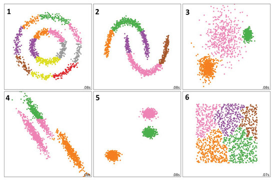
Figure 1.
Results of the proposed approach made on datasets from scikit-learn.
Figure 1 allows for two conclusions. First, for three-cluster datasets, our method works well, the results are close to the Ward method, but work even better with borderline units (see visualizations for the datasets 3, 4, and 5, in comparison with the respective visualizations at scikit-learn for the Ward method). The visualization confirms that our method suits well for the datasets with three or more clusters. In this respect, the dataset 3 at Figure 1 deserves particular attention. This dataset contains three spherical clusters with fuzzy boundaries (compare to the dataset 5). Such distribution of points in a Euclidean space is typical for text representations by normalized vectors (e.g., embeddings-based representations). If we a priori assume that, according to the Euclidean metric, similar texts have similar vector representations, they should form spherical clusters. At the same time, the problem of fuzzy boundaries between different types of texts is well-known. According to Snell-Hornby [26], there are no clear boundaries between types of texts, but only a certain center for each of the types. Therefore, we can assume that the representation of textual data by normalized vectors in the Euclidean space most closely matches the one of the dataset 3 at Figure 1. Additionally, this is exactly where our method works best. Second, for the datasets with one or two clusters, our method detects a big number of clusters (see visualizations for the datasets 1, 2, and 6 at Figure 1). This proves that use of the “e-2” hypothesis allows for catching the moment when the clustering process begins, before the chain effect shows up. Again, this proves that our method is suitable for datasets with large number of clusters, like the real-world ones used for topic detection.
Now, let us see how the “e-2” hypothesis works in comparison with more traditional ways of stopping to determine the preferred number of clusters, namely the silhouette metric and the elbow method. Our approach differs from both of them. The elbow method is a heuristic used to determine the number of clusters in a dataset. It consists of finding the “elbow” of the graph of change as a function of the number of clusters. The most common variation that is used in the elbow method is total variance within the cluster. The proposed method for determining the number of clusters using approximation-estimation tests is also based on finding the “elbow” of the graph of some values that characterize the clustering process. The difference is that the definition number of clusters with help of “elbow” is based upon heuristic visual assessment, but the definition number of clusters with help of approximation-estimation tests and “e-2” hypothesis is based upon sequential statistical analysis.
Unlike the elbow method, the silhouette coefficient is non-heuristic. It is based on two scores: is the average distance from current point x to objects of its own cluster A, and is the average distance from the current point x to the objects of cluster B, which is the closest one to x. The silhouette coefficient of point x is the number :
It is easy to see that . The value of s(x) being close to 1 implies that the point is clustered well; the value being close to implies that the point is clustered incorrect. If the value is close to 0, it it means that the distances from x to both clusters A and B are the same, and the point x should be assigned to either A or B. This case can be considered as “ntermediate”. The silhouette coefficient of a dataset is defined as the average of the silhouette coefficients for all of the points of the sample. The number of clusters with the highest silhouette coefficient for the fixed clustering method can be determined as the optimal number of clusters for this method applied to the dataset under scrutiny [27].
However, the silhouette coefficient has its shortcomings. It takes much time to compute the silhouette coefficients for every data unit in large datasets for every possible clustering result. Additionally, the silhouette coefficient cannot detect well the original number of clusters if the clusters overlap and have fuzzy boundaries, while our method helps to eliminate this problem.
To prove it, we have applied our method to another well-known model dataset, namely the iris dataset (https://scikit-learn.org/stable/modules/generated/sklearn.datasets.load_iris.html#sklearn.datasets.load_iris). The results of the application are shown in Table 1 and Table 2 (the silhouette coefficient and “e-2” hypothesis, respectively). The iris dataset consists of data of three classes, with two of them slightly overlapping, and our features for each data unit. Thus, the expected number of clusters is three. The results presented in Table 1 and Table 2 clearly show that the silhouette coefficient misses the point in detecting the right number of clusters, while our method finds the right number of clusters on the interval of stable clustering “e-2”.

Table 1.
The number of clusters received for the iris dataset by the silhouette coefficient.
Table 2.
The number of clusters received for the iris dataset by application of the e-2 hypothesis.
4. The Experiment against the Baselines and Its Results
The tests were performed on two distinct datasets. News20 is a dataset containing news headlines and articles, which was split into four subsets. Each division contains rows with unique labels e.g., rows from a subset containing three classes is not used in subsets with five and 10 classes. BBC is a dataset containing BBC articles with each row labeled as one of the five distinct classes: sport, tech, business, entertainment, and politics.
The proposed model was tested against two other well-known clustering methods that have the ability to infer the optimal number of clusters as part of the training process. DBSCAN and OPTICS were chosen as one of the few classic approaches that does not require the number of clusters to train the model [28,29].
Three metrics were utilized to evaluate the performance of our method against classic approaches. The V-measure can be described as a weighted harmonic mean of homogeneity and completeness [30]. In this metric, the homogeneity criterion is satisfied if the algorithm only assigns to a single cluster the data units that are members of a single class. In order to satisfy the completeness criteria, the algorithm must assign to a single cluster all of the data units that are members of a single class. NMI (Normalized Mutual Information) [31] was used as additional performance metric, which utilises entropies of class labels and mutual information (a reduction in the entropy of class labels after training). Both of these metrics are independent of the absolute values of the labels, and the results of clustering can be directly compared with the true labels, which are document classes of the original data assigned by the authors of this dataset. Finally, to test models’ ability to accurately determine the number of clusters in a given corpus, we employed a measure of similarity between the optimal number of clusters and the number obtained by algorithms (number of clusters’ inference accuracy).
Experiments were conducted with different encoding techniques, in order to test their possible impact on the model’s performance. The first model is TF-IDF, as it is, to this day, a very popular encoding methods for relatively simple tasks. Another employed method is FastText [32], which is an extension of a well-known word2vec model with improved accuracy and faster training time due to the usage of negative sampling. Finally, we use the context-aware USE model described in Section 2, which, unlike FastText, can output embeddings not just for words but for entire sentences and, by doing so, bypasses the process of averaging the word embeddings typically performed by the models that do not utilise context information, such as FastText.
The results for different combinations of training and encoding models, as well as different metrics, can be seen in Table 3, Table 4, Table 5, Table 6, Table 7, Table 8 and Table 9.
Table 3.
V-measure for News3 and News5.
Table 4.
V-measure for News10 and News20.
Table 5.
NMI for News3 and News5.
Table 6.
NMI for News10 and News20.
Table 7.
The number of clusters’ inference accuracy for News3 and News5.
Table 8.
The number of clusters’ inference accuracy for News10 and News20.
Table 9.
Results for BBC dataset (Universal Sentence Encoder (USE) data pre-processing).
The experiment shows that the proposed method of agglomerative clustering with USE pre-processing provides a much better result when compared to the baselineS, namely DBSCAN and OPTICS. The model performs especially well when the number of classes increases, reaching eight-times better performance than the baseline model if compared by the V-measure.
5. Discussion
As we have demonstrated above, the proposed method shows high efficiency against the baseline; however, it is not deprived of shortcomings.
As for data pre-processing and the dataset, the most notable downside to models, such as USE, are their requirements in terms of hardware and their time-consuming nature. This is especially true then the model is trained from scratch, but even the inference process can be rather slow then dealing with large corpora. Additionally, News20 has very well-defined classes and, as such, may not be representative of the performance on the real data. However, it provides a good enough estimate of the model performance by giving us the ability to check the clustering performance via comparing obtained cluster labels with the true labels defined for this set by human coding.
As for the clustering procedure with the Markov moment, it still possesses some residual subjectivity, as sensitivity of the stopping criterion may be changed by the researcher. As we noted above, clustering per se is a subjective instrument when used for topicality or sentiment detection, as almost all of the stopping criteria (that is, the criteria for selection of the optimal number of clusters) are subjective by nature, being based on heuristic approaches to problem resolution. The use of “e-2 hypothesis” that we have suggested above aims at reducing the level of subjectivity. Additionally, more experiments are needed to collect empirical data on the optimal values of the stopping criterion for the real-world data. In order to overcome the problem of subjectivity, the data might as well undergo further experiments with various procedures for stopping, while the results might be compared to expert opinion, given that the level of agreement of 0.7–0.8 among the human coders is reached. However, we need to note that our prior experiments with topic models and human coding have shown that manual coding should not be taken as baseline. In particular, for pairs of human coders, topic interpretability and proximity varied for over 10 times, depending on prior familiarity with the dataset and coding experience [33]. Thus, the quality assessment of clustering remains an issue. Our approach significantly helps researchers to reduce subjectivity but does not eliminate it completely. The advantage of our approach is that it allows for testing subtle changes in topicality distribution by nuanced variances of the stopping criterion, rather than changing the number of topic slots in arbitrary manner.
Possible limitations of our work may also lie in two aspects. The utilization of transformer-based sentence embeddings and USE may be advised to scholars interested in text clustering, but application of USE may be technically unfeasible for some of them. Additionally, the limitations might be linked to the nature of the datasets, which, as mentioned before, stands between regularized text collections and highly noisy data from social media.
6. Conclusions
Above, we have demonstrated the efficiency of a combined method for automated text typology that unites the tasks of text classification and text clustering. We have used sentence embeddings at the stage of pre-processing and hierarchical agglomerative clustering with an approximation-estimation test and the Markov stopping moment for defining the time of completion of clustering.
We have shown that this methodological design showed high efficiency in comparison with two baselines, DBSCAN and OPTICS. It is especially true for the number of clusters higher than five. The quality of the model does not drop at 10 and 20 classes, which allows overcoming the well-known problem of low performance of text classification for high numbers of clusters. The results may be applied to a wide array of tasks of text classification, including topic detection, multi-class sentiment analysis, and clustering of multilingual datasets by language. In combination with social network analysis, it may be applied for community detection on social networks and to other tasks of networked discussion analytics.
Real-world data can pose challenges to our method, as mentioned above. Thus, our future work will develop in three directions. First, we will apply the proposed method to the real-world datasets from unilingual and multilingual Twitter and Youtube that we have collected in 2014 to 2019 [34]. We expect the results to drop to some extent, as the real-world data substantially complicate pre-processing. This is why, second, our future work will involve testing the model with other encoding methods such as XLNet, BERT, and others. Third, testing the model against other, more specialized clustering models and comparing them with the help of a wide array of metrics can also provide for better understanding of the efficiency of the model.
Author Contributions
Conceptualization, A.V.O., S.S.B.; Methodology, A.V.O., I.S.B.; Software, I.S.B.; Validation, I.S.B., N.A.T., N.S.L.; Data Curation, I.S.B., N.A.T., N.S.L.; Writing—Original Draft Preparation, S.S.B., A.V.O., I.S.B.; Writing—Editing, S.S.B.; Project Administration, S.S.B.; Funding Acquisition, S.S.B. All authors have read and agreed to the published version of the manuscript.
Funding
This work was supported in full by Russian Science Foundation, grant number 16-18-10125-P.
Conflicts of Interest
The authors declare no conflict of interest.
Appendix A. Method Application and Quality Assessment
Below, we provide a tutorial for the method application.
Appendix A.1. Encodings
First, the initial rows of sentences are pre-processed for tf-idf representation using nltk.PorterStemmer for stemming and stop_words.get_stop_words for stop words removal. After that, the data are transformed to the vector form using sklearn.feature_extraction.text.TfidfVectorizer for further clustering. FastText and USE encoding models, at their core, do not rely on distinct words to encode sentences (instead, they utilize subword information). Thus, they do not need any pre-processing at the beginning. FastText encoding is obtained using fasttext.util.download_model with the pre-trained model ’cc.en.300.bin’. For the USE encoding, tensorflow_hub.load is utilized to load the default v4 version of the model (https://tfhub.dev/google/universal-sentence-encoder/4).
Appendix A.2. Baseline Models
The next step is to obtain the baseline models for testing. sklearn.cluster.DBSCAN and sklearn.cluster.OPTICS are used to train the DBSCAN and OPTICS models, respectively. In almost all cases, the models are used with their default parameters for text clustering. Using hyper optimisation methods was considered; however, it made more sense to compare the models without changing their parameters from case to case, to be on the leveled field with the proposed model which is trained only once for each case—that is, without any further hyperparameter optimisation.
Appendix A.3. The Proposed Model
The proposed approach is based on the Ward method of agglomerative clustering. scipy.cluster.hierarchy.ward is used to get the linkage matrix. The column with index 2 of this matrix is a set of minimum distances. It can be easily transformed into a trend set by adding numpy.arange multiplied on q to it. It is possible to find the stopping moment via brute force method, by sequentially increasing the coefficient q with a fixed step. For each value of q, find all stopping moments sequentially checking the sign of approximation-estimation test for elements of trend set built with q. Stop the process of searching if the value of q is so high that, for every row of the linkage matrix, the approximation-estimation test is taking non-positive values and there is no stopping moment. Then use scipy.cluster.hierarchy.fcluster to get cluster labels for the stopping moment using information from the linkage matrix, e.g., the minimum distance or the number of clusters on this step.
Appendix A.4. Brief Description of the Algorithm
| Algorithm A1: Step-by-step instructions of use |
|
Appendix A.5. Quality Measurements
The last step in the experiment is measuring the performance of each model using NMI and VM scores, which is done using sklearn.metrics.cluster. The resulting vector of cluster labels is compared to the initial target vector. An additional metric, namely the number of clusters’ inference accuracy, is also used to measure how similar the inferred number of clusters is to their real number. The latter metric is calculated as a simple relative difference between these two values.
References
- Nikolenko, S.I.; Koltcov, S.; Koltsova, O. Topic modelling for qualitative studies. J. Inf. Sci. 2017, 43, 88–102. [Google Scholar] [CrossRef]
- Bodrunova, S.S. Topic modelling in Russia: Current approaches and issues in methodology. In The Palgrave Handbook of Digital Russia Studies; Gritsenko, D., Wijermars, M., Kopotev, M., Eds.; Palgrave Macmillan: London, UK. (in print)
- Greene, D.; O’Callaghan, D.; Cunningham, P. How many topics? Stability analysis for topic models. In Proceedings of the Joint European Conference on Machine Learning and Knowledge Discovery in Databases, Nancy, France, 15–19 September 2014; Springer: Berlin/Heidelberg, Germany, 2014; pp. 498–513. [Google Scholar]
- Blei, D.M.; Ng, A.Y.; Jordan, M.I. Latent dirichlet allocation. J. Mach. Learn. Res. 2003, 3, 993–1022. [Google Scholar]
- Symeonidis, S.; Effrosynidis, D.; Arampatzis, A. A comparative evaluation of pre-processing techniques and their interactions for twitter sentiment analysis. Expert Syst. Appl. 2018, 110, 298–310. [Google Scholar] [CrossRef]
- Mittal, M.; Goyal, L.M.; Hemanth, D.J.; Sethi, J.K. Clustering approaches for high?dimensional databases: A review. Wiley Interdiscip. Rev. Data Min. Knowl. Discov. 2019, 9, e1300. [Google Scholar] [CrossRef]
- Orekhov, A.V.; Kharlamov,, A.A.; Bodrunova,, S.S. Network presentation of texts and clustering of messages. In Proceedings of the 6th International Conference on Internet Science, Perpignan, France, 2–5 December 2019; El Yacoubi, S., Bagnoli, F., Pacini, G., Eds.; Lecture Notes in Computer Science (LNCS). Springer: Cham, Switzerland, 2019; Volume 11938, pp. 235–249. [Google Scholar]
- Kharlamov, A.A.; Orekhov,, A.V.; Bodrunova,, S.S.; Lyudkevich,, N.S. Social Network Sentiment Analysis and Message Clustering. In Proceedings of the 6th International Conference on Internet Science, Perpignan, France, 2–5 December 2019; El Yacoubi, S., Bagnoli, F., Pacini, G., Eds.; Lecture Notes in Computer Science (LNCS). Springer: Cham, Switzerland, 2019; Volume 11938, pp. 18–31. [Google Scholar]
- Bodrunova, S.S.; Blekanov, I.S.; Kukarkin, M. Topics in the Russian Twitter and relations between their interpretability and sentiment. In Proceedings of the Sixth International Conference on Social Networks Analysis, Management and Security (SNAMS), Granada, Spain, 22–25 October 2019; pp. 549–554. [Google Scholar]
- Greene, D.; Cunningham, P. Practical Solutions to the Problem of Diagonal Dominance in Kernel Document Clustering. In Proceedings of the 23rd International Conference on Machine learning (ICML’06), Pittsburgh, PA, USA, 25–29 June 2006; ACM Press: New York, NY, USA, 2006; pp. 377–384. [Google Scholar]
- Cer, D.; Yang, Y.; Kong, S.Y.; Hua, N.; Limtiaco, N.; John, R.S.; Constant, N.; Guajardo-Cespedes, M.; Yuan, S.; Tar, C.; et al. Universal Sentence Encoder for English. In Proceedings of the 2018 Conference on Empirical Methods in Natural Language Processing: System Demonstrations, Brussels, Belgium, 31 October–4 November 2018; pp. 169–174. [Google Scholar]
- Aharoni, R.; Goldberg, Y. Unsupervised Domain Clusters in Pretrained Language Models. arXiv 2020, arXiv:2004.02105. [Google Scholar]
- Everitt, B.S. Cluster Analysis; John Wiley & Sons Ltd.: Chichester, West Sussex, UK, 2011. [Google Scholar]
- Duda, R.O.; Hart, P.E.; Stork, D.G. Pattern Classification, 2nd ed.; John Wiley & Sons Ltd.: New York, NY, USA; Chichester, West Essex, UK, 2001. [Google Scholar]
- Orekhov, A.V. Markov stopping time of an agglomerative clustering process in Euclidean space. Vestn. St.-Peterbg. Univ. Prikl. Mat. Inform. Protsessy Upr. 2019, 15, 76–92. (In Russian) [Google Scholar] [CrossRef]
- Orekhov, A.V. Agglomerative Method for Texts Clustering. In Proceedings of the 5th International Conference on Internet Science (INSCI 2018), St. Petersburg, Russia, 24–26 November 2018; Bodrunova, S., Ed.; Lecture Notes in Computer Science (LNCS). Springer: Cham, Switzerland, 2019; Volume 11551, pp. 19–32. [Google Scholar] [CrossRef]
- Van der Waerden, B.L. Algebra; Springer: New York, NY, USA, 1991; Volume 1, p. 265. [Google Scholar]
- Lang, S. Algebra; Springer: New York, NY, USA, 2002; p. 914. [Google Scholar]
- Aldenderfer, M.S.; Blashfield, R.K. Cluster Analysis: Quantitative Applications in the Social Sciences; Sage Publications: Beverly Hills, CA, USA, 1984. [Google Scholar]
- Hartigan, J.A. Clustering Algorithms; John Wiley & Sons: New York, NY, USA; London, UK, 1975. [Google Scholar]
- Wald, A. Sequential Analysis; John Wiley & Sons: New York, NY, USA, 1947. [Google Scholar]
- Sirjaev, A.N. Statistical Sequential Analysis: Optimal Stopping Rules; American Mathematical Society: Providence, RI, USA, 1973; Volume 38. [Google Scholar]
- Orekhov, A.V. Criterion for estimation of stress-deformed state of SD-materials. In AIP Conference Proceedings; AIP Publishing LLC: College Park, MD, USA, 2018; Volume 1959, p. 70028. [Google Scholar] [CrossRef]
- Orekhov, A.V. Approximation-evaluation criteria for the stress-strain state of a solid body. Vestn. St.-Peterbg. Univ. Prikl. Mat. Inform. Protsessy Upr. 2018, 14, 230–242. (In Russian) [Google Scholar] [CrossRef]
- Granichin, O.N.; Shalymov, D.S.; Avros, R.; Volkovich, Z. A randomized algorithm for estimating the number of clusters. Autom. Rem. Contr. 2011, 72, 754–765. [Google Scholar] [CrossRef]
- Snell-Hornby, M. Translation Studies: An Integrated Approach; John Benjamins Publishing: Amsterdam, The Netherlands, 1988; p. 172. [Google Scholar]
- Rousseeuw, P.J. Silhouettes: A graphical aid to the interpretation and validation of cluster analysis. J. Comput. Appl. Math. 1987, 20, 53–65. [Google Scholar] [CrossRef]
- Ester, M.; Kriegel, H.P.; Sander, J.; Xu, X. A density-based algorithm for discovering clusters in large spatial databases with noise. Kdd 1996, 96, 226–231. [Google Scholar]
- Schubert, E.; Gertz, M. Improving the Cluster Structure Extracted from OPTICS Plots; LWDA: Mannheim, Germany, 2018; pp. 318–329.
- Rosenberg, A.; Hirschberg, J. V-measure: A conditional entropy-based external cluster evaluation measure. In Proceedings of the 2007 Joint Conference on Empirical Methods in Natural Language Processing and Computational Natural Language Learning (EMNLP-CoNLL), Prague, Czech Republic, 28–30 June 2007; Eisner, J., Ed.; ACL: Stroudsburg, PA, USA, 2007; pp. 410–420. [Google Scholar]
- Strehl, A.; Ghosh, J. Cluster ensembles—A knowledge reuse framework for combining multiple partitions. J. Mach. Learn. Res. 2002, 3, 583–617. [Google Scholar]
- Bojanowski, P.; Grave, E.; Joulin, A.; Mikolov, T. Enriching word vectors with subword information. Trans. Assoc. Comput. Linguist. 2017, 5, 135–146. [Google Scholar] [CrossRef]
- Blekanov, I.S.; Bodrunova, S.S.; Zhuravleva, N.; Smoliarova, A.; Tarasov, N. The Ideal Topic: Interdependence of Topic Interpretability and other Quality Features in Topic Modelling for Short Texts. In Proceedings of the HCI International 2020, Copenhagen, Denmark, 19–24 July 2020; Lecture Notes in Computer Science (LNCS). Springer: Cham, Switzerland, 2020; pp. 19–26. [Google Scholar]
- Bodrunova, S.S.; Blekanov, I.; Smoliarova, A.; Litvinenko, A. Beyond left and right: Real-world political polarization in Twitter discussions on inter-ethnic conflicts. Media Commun. 2019, 7, 119–132. [Google Scholar] [CrossRef]
© 2020 by the authors. Licensee MDPI, Basel, Switzerland. This article is an open access article distributed under the terms and conditions of the Creative Commons Attribution (CC BY) license (http://creativecommons.org/licenses/by/4.0/).